A critical review of statistical
calibration/prediction models handling
data inconsistency and model inadequacy

Abstract

Inference of physical parameters from reference data is a well studied problem with many intricacies (inconsistent sets of data due to experimental systematic errors; approximate physical models…). The complexity is further increased when the inferred parameters are used to make predictions – virtual measurements – because parameters uncertainty has to be estimated in addition to parameters best value. The literature is rich in statistical models for the calibration/prediction problem, each having benefits and limitations.

We review and evaluate standard and state-of-the-art statistical models in a common bayesian framework, and test them on synthetic and real datasets of temperature-dependent viscosity for the calibration of Lennard-Jones parameters of a Chapman-Enskog model.

CNRS, UMR8000, Laboratoire de Chimie Physique, F-91405 Orsay, France

Univ. Paris-Sud, UMR000, Laboratoire de Chimie Physique, F-91405 Orsay, France

Contact: pascal.pernot@u-psud.fr

1 Introduction

The past decades have seen a tremendous increase in the size and time-scales of molecular systems accessible to computational chemistry. Estimation of the prediction uncertainty of such simulations is the next challenging step to reach virtual measurements [1], i.e., to enable simulations or physical modelsTwo types of models are referred to in this study: physical (or knowledge) models used to make predictions of physico-chemical properties and statistical models used to calibrate the knowledge models. Most of the times, the simple term model will be used when there is no ambiguity. The same holds for the parameters of both types of models. to replace experiments. This subject is taking momentum in the computational chemistry community, and several studies have been reported recently in the literature, mostly in the last 5 years, and notably for atomistic/molecular simulation [3, 4, 5, 6, 7, 8, 9], density functional theory [10, 11, 12, 13, 14, 15, 16], quantum chemistry [17, 18] and multiscale catalysis studies [19, 20, 21]. Chemical engineering is a companion field where uncertainty quantification (UQ) is becoming crucial [22, 23, 24, 25, 26, 27, 28, 29, 30, 31, 32, 21].

The estimation of model prediction uncertainty (MPU) is a complex process, which requires a careful analysis of the main error sources: (i) systematic errors due to the model formulation and approximations (model inadequacy); (ii) numerical errors (notably for stochastic models); and (iii) parameter uncertainty. Once the error sources are well identified and quantified, uncertainty propagation to model predictions is rather straightforward, even if often computationally challenging [33, 34, 35].

Except for stochastic or chaotic models, numerical errors are expected to be well controlled and kept to a negligible level [1, 36, 37]. The remaining sources depend on comparisons with reference data: parameter uncertainty is generally the result of a model calibration process by which the parameters are identified; and quantification of a model’s systematic errors requires reference data. As reference data are generally experimental, measurement errors, both systematic and random, contaminate to some extent the estimation of model error sources [14].

In this study, we focus on the estimation of prediction uncertainty in the typical calibration/prediction scenario, where one is faced with inconsistent reference data and an approximate or misspecified model:

• Data inconsistency occurs when the scatter of repeated measurements is statistically inconsistent with the stated uncertainty of the individual measurements [38, 39]. This is an ubiquitous problem in the comparison of data produced by different laboratories and/or different measurement setups. It might result from incorrect quantification of measurement uncertainty, but often has its origin in unidentified systematic errors in the measurement process. If the data are abundant, one has the option to reject data until one obtains a consistent dataset [40]. In this context, rejecting outliers is always dangerous, as they might in fact be the nearest to the true value. Recently, metrologists have developed statistical methods enabling to preserve all data, notably through the use of bayesian hierarchical models [41, 39, 42].

• Model inadequacy results from approximations at various stages of model development and is responsible for systematic errors in predictions [43]. It should be identified and quantified by comparison with reference data. Correction of model systematic errors can be done by model improvement, or by a posteriori correction of model predictions [14]. Model improvement is often impractical or impossible, and the latter option is popular, for instance, in the statistical correction of harmonic vibrational frequencies by scaling [44, 45]. If model inadequacy cannot be corrected, it is essential that prediction uncertainty be large enough to account for it. This leads to several options in prediction uncertainty modeling reviewed recently by Sargsyan et al.,[46] and that will be considered in the following.

The systematic errors linked to model inadequacy have a major impact on the parameters recovered when calibrating the model, which is difficult to unmix from the impact of data inconsistency [31]. In order to establish a reliable MPU, it is necessary to discriminate correctly the error sources and their degeneracy in the model calibration process, by the design of an adequate statistical calibration/prediction process.

Our aim in the present study is to review the main approaches used in the computational chemistry literature to deal with data inconsistency and/or model inadequacy. For instance, Wu et al. [9] recently proposed a hierarchical model to calibrate the Lennard-Jones parameters of an interatomic potential on inconsistent viscosity measurements. Their use of physical parameters to represent systematic experimental errors is intriguing and needs further consideration.

Assuming a valid calibration/prediction process, the question remains of the transferability of model calibration to other observables [47, 48]. All calibration methods based on the a posteriori correction of model predictions are by nature not transferable. A solution to the transferability problem is to affect to the model’s parameters uncertainty the prediction errors due to model inadequacy.[46] This has been done in various ways: uncertainty scaling [10, 11, 13], embedded stochastic models [46, 30] and hierarchical models [9]. Parameters and their enlarged uncertainty are then transferable, but this approach is not without drawbacks [32, 49]: the transfer of parameter uncertainty to MPU is governed by the functional shape (with respect to the control variables) of the model sensitivity coefficients. This leads to confidence bands with a model-specific shape, not necessarily representative of the actual model errors. As demonstrated, for instance, in the case of scaling factors for harmonic frequencies, or in the calibration of the mBEEF density functional, the mean MPU is, by design, in good agreement with the error statistics, but individual MPUs are unreliable, being over- or under-estimated in different parts of the control space [49].

This paper attempts a critical review of classical and state-of-the-art statistical models dealing with data inconsistency and model inadequacy. For presentation consistency, the statistical models are cast in the bayesian framework introduced in Section 2. The models themselves are presented in Section 3. We then consider the advantages and limitations of each method (and their combinations), illustrated on the calibration of the parameters of a Lennard-Jones potential from synthetic and experimental viscosity data (Section 4). The discussion (Section 5) draws on these examples to propose guidelines for a successful calibration/prediction process.

2 Statistical methods

Some of the simpler calibration/prediction methods are commonly presented in a least-squares framework, whereas the most sophisticated ones rely on a bayesian formulation. For homogeneity, the latter has been used throughout this study, and we provide a short introduction below. More detailed presentations of bayesian data analysis can be found in textbooks [50, 51, 52].

2.1 Bayesian calibration and prediction

One considers a model represented by the function $M(x;\boldsymbol{\vartheta})$Boldface type refers to vectors or matrices., depending on a (set of) control variable(s) $x$ (e.g. temperature, pressure…), and parameters $\boldsymbol{\vartheta}$ that have to be identified, i.e. characterized by their probability density function (pdf) or, in the gaussian hypothesis, their “best” value and covariance matrix [43]. Parameters inference is done by calibration of the model on a set of reference data $\boldsymbol{D}$.

The posterior probability density function $p(\boldsymbol{\vartheta}|\boldsymbol{D},M)$ for the parameters $\boldsymbol{\vartheta}$, conditional on $\boldsymbol{D}$ and $M$, is provided by Bayes formula

$$p(\boldsymbol{\vartheta}|\boldsymbol{D},M)=\frac{p(\boldsymbol{D}|\boldsymbol{\vartheta},M)\,p(\boldsymbol{\vartheta}|M)}{p(\boldsymbol{D}|M)},$$ (1)

where

• $p(\boldsymbol{D}|\boldsymbol{\vartheta},M)$ is the likelihood function, describing the distribution of the differences between model and data, as detailed below;

• $p(\boldsymbol{\vartheta}|M)$ is the prior pdf of the parameters, to be defined later;

• $p(\boldsymbol{D}|M)$ is the evidence, a normalization constant which we do not need to estimate in the following.

For simpler notations, $M$ will be kept implicit in the following.

The mode of the posterior pdf, $\hat{\boldsymbol{\vartheta}}$, or maximum a posteriori ($MAP$) solution, provides an estimate of the “best fit” solution of the calibration problem. The mean value of the parameters $\boldsymbol{\mu}_{\vartheta|D}$ and their covariance matrix $\boldsymbol{V}_{\vartheta|D}$ are often used to summarize the posterior pdf.

The full posterior pdf is necessary to account for parameter uncertainty in prediction of the true value $\tilde{y}$ at a new control point $\tilde{x}$ through the posterior predictive distribution

$$p_{M}(\tilde{y}|\tilde{x},\boldsymbol{D}) = \int f(\tilde{y}|\tilde{x},\boldsymbol{\vartheta})\,p(\boldsymbol{\vartheta}|\boldsymbol{D})\,d\boldsymbol{\vartheta},$$ (2)

where $f(\tilde{y}|\tilde{x},\boldsymbol{\vartheta})$ is a probability density function which might be a Dirac function $f(\tilde{y}|\tilde{x},\boldsymbol{\vartheta})=\delta\left(\tilde{y}-M(\tilde{x};\boldsymbol{\vartheta})\right)$, if there is no model uncertainty [34], or a pdf describing $\tilde{y}$ as the output of a random process characterizing model errors [51]. For deterministic models, the mean value of a prediction at a new control value $\tilde{x}$ and its variance can be approximated by linear uncertainty propagation[33]

$$\mu_{M|D}(\tilde{x}) =M(\tilde{x};\boldsymbol{\mu}_{\vartheta|D})$$ (3)

$$u_{M|D}^{2}(\tilde{x}) =\boldsymbol{J}^{T}(\tilde{x};\boldsymbol{\mu}_{\vartheta|D})\boldsymbol{V}_{\vartheta|D}\boldsymbol{J}(\tilde{x};\boldsymbol{\mu}_{\vartheta|D}),$$ (4)

where $\boldsymbol{J}$ is a vector of sensitivity coefficients

$$\boldsymbol{J}_{k}(x;\boldsymbol{\mu}_{\vartheta|D})=\left.\frac{\partial M(x;\boldsymbol{\vartheta})}{\partial\boldsymbol{\vartheta}_{k}}\right|_{\boldsymbol{\mu}_{\vartheta|D}}.$$ (5)

In order to predict a new experimental measurement, $p_{M}(\tilde{y}|\tilde{x},\boldsymbol{D})$ has to be convoluted with the pdf describing expected measurement errors, $p(\tilde{y_{e}}|\tilde{y})$:

$$p_{e}(\tilde{y_{e}}|\tilde{x},\boldsymbol{D}) = \int p(\tilde{y_{e}}|\tilde{y})\,p_{M}(\tilde{y}|\tilde{x},\boldsymbol{D})\,d\tilde{y}.$$ (6)

In the linear uncertainty propagation framework, one would get the variance of prediction $\tilde{y_{e}}$ as

$$u_{e|D}^{2}=u_{M|D}^{2}+u_{y_{e}}^{2},$$ (7)

where $u_{y_{e}}^{2}$ is the measurement variance for $\tilde{y_{e}}$.

2.1.1 The likelihood

For all models used in this study, we assume errors with normal distributions, in which case the likelihood function can be expressed as a multivariate normal distribution

$$p(\boldsymbol{D}|\boldsymbol{\vartheta}=\left\{\boldsymbol{\vartheta}_{M},\boldsymbol{\vartheta}_{V}\right\})=\frac{1}{\left(\sqrt{2\pi}\right)^{N}\left|\boldsymbol{V}\right|^{1/2}}\exp\left(-\frac{1}{2}\boldsymbol{R}^{T}\boldsymbol{V}^{-1}\boldsymbol{R}\right),$$ (8)

where

• $\boldsymbol{R}$ is a $N$-vector of residuals $R_{i}=y_{i}-M(x_{i};\boldsymbol{\vartheta}_{M})$, and

• $\boldsymbol{V}$ is a $N\times N$ covariance matrix, possibly parameterized by $\boldsymbol{\vartheta}_{V}$.

The latter has typically a contribution $\boldsymbol{V}_{D}$ built from experimental measurement covariances, and, in some cases, a contribution $\boldsymbol{V}_{M}$ characterizing model errors

$$\boldsymbol{V}=\boldsymbol{V}_{D}+\boldsymbol{V}_{M}.$$ (9)

In the Approximate Bayesian Computing approach, this expression of the likelihood might be different, as discussed in 3.3.2.2.2.

2.1.2 Validation

Noting $\boldsymbol{\hat{R}}$ the residuals at the $MAP$, $\hat{\boldsymbol{\vartheta}}$, one defines the mean squared residuals ($MSR$), mean residuals ($MR$), root mean squared deviation ($RMSD$):

$$MSR = \frac{1}{N}\sum_{i=1}^{N}\hat{R}_{i}^{2},$$ (10)

$$MR = \frac{1}{N}\sum_{i=1}^{N}\hat{R}_{i},$$ (11)

$$RMSD = \sqrt{MSR-MR^{2}}.$$ (12)

A convenient validation statistics accounting for the covariance structure of the statistical model is the Birge ratio $R_{B}$,[54, 55]

$$R_{B} = \frac{1}{N-\nu}\boldsymbol{\hat{R}}^{T}\boldsymbol{V}^{-1}\boldsymbol{\hat{R}},$$ (13)

where $\nu$ is the number of degrees of freedom of the fit. $R_{B}$ is a dimensionless quantity, which should be close to $1$ when calibration is statistically sound. A limitation of $R_{B}$ is that for complex statistical models, such as hierarchical models or gaussian processes, $\nu$ is not easily estimated.

Various prediction statistics can be used also for validation [56, 51, 48]. Posterior predictive assessment compares model predictions with reference data and/or validation data.

Using the calibration dataset $\boldsymbol{D}=\{x_{i},y_{i},u_{i};\,i=1,\,N\}$ for validation, one defines the mean prediction variance as

$$MPV=\frac{1}{N}\sum_{i=1}^{N}\left(u_{M}^{2}(x_{i},\boldsymbol{D})+u_{i}^{2}\right),$$ (14)

where $u_{M}(x_{i},\boldsymbol{D})$ is the standard deviation of $p_{M}(\tilde{y}|x_{i},\boldsymbol{D})$ and $u_{i}$ is the measurement uncertainty on $y_{i}$. The mean prediction uncertainty is noted

$$u_{e|D}=\sqrt{MPV}.$$ (15)

In absence, or after correction, of data inconsistency, the residuals result from model inadequacy and data uncertainty. In such cases, one should thus expect that

$$u_{e|D}\gtrsim RMSD.$$ (16)

As evoked in the introduction, mean statistics can hide underlying problems, and it is always important to perform a visual check of the prediction bands, built at a series of points $\tilde{x}$ in control space from prediction uncertainties $u_{M}(\tilde{x},\boldsymbol{D})$ and $u_{e}(\tilde{x},\boldsymbol{D})$, the standard deviation of $p_{M}(\tilde{y}|\tilde{x},\boldsymbol{D})$ and $p_{e}(\tilde{y}|\tilde{x},\boldsymbol{D})$, respectively.

2.2 Implementation

The bayesian models are implemented in Stan [57], using the rstan interface package for R [58]. Stan is a very flexible and efficient probabilistic programming language to implement bayesian statistical models, including advanced ones, such as Hierarchical Models, Gaussian Processes or Approximate Bayesian Computation (ABC).

The main outputs are samples of the posterior pdf and posterior predictive pdf, from which statistics and plots can be generated in R. We used the No-U-Turn sampler [59] throughout this study. Convergence of the sampling was assessed by examining the parameters samples and the split Rhat statistics provided by rstan.

Uniform prior pdfs have been used for location parameters, and log-uniform for scaling parameters, unless stated explicitly. All models were run with 4 parallel Markov Chains of 5000 iterations each, 1000 of which are used as warm-up for the No-U-Turn sampler. The convergence criteria and parameters statistics are thus estimated on four samples of 4000 points.

The data and codes necessary to reproduce the results of the present study are provided as Supporting Information.

3 Calibration models

One considers a calibration set of $N$ data points issued from $N_{s}$ experimental series, $\boldsymbol{D}=\{d_{i};\,i=1,\,N\}$ with $d_{i}=(x_{i},y_{i},u_{i},\kappa_{i})$, where $x_{i}$ and $y_{i}$ are the values of the control and measured variables, $u_{i}$ is the corresponding measurement uncertaintyThe uncertainty on the control variable is assumed to be negligible in all experiments., and $\kappa_{i}\in 1:N_{s}$ is the series index of datum $i$. An experimental measurement series is noted $D^{(j)}$, and its cardinal is noted $n^{(j)}$.

We first consider the simplest statistical model as a basis for the definition and discussion of more elaborate models accounting for data inconsistency and model inadequacy.

3.1 Std: standard model

The most basic model (named Std in the following) treats all data in a single series ($N_{s}=1$), with equal and unknown uncertainty. The set of calibration parameters comprises the model parameters $\boldsymbol{\vartheta}_{M}$ and a parameter $\vartheta_{V}=\sigma$, accounting for the dispersion of residuals. Assuming independent errors with normal distribution

$$y_{i} =M(x_{i};\boldsymbol{\vartheta}_{M})+\epsilon_{i},$$ (17)

$$\epsilon_{i} \sim\mathcal{N}(0,\sigma^{2}),$$ (18)

the elements of $\boldsymbol{R}$ and $\boldsymbol{V}$ (Eq. 8) are

$$R_{i} = y_{i}-M(x_{i};\boldsymbol{\vartheta}_{M}),$$ (19)

$$V_{ij} = \sigma^{2}\delta(i-j).$$ (20)

In absence of prior information on the parameters, this method is akin to Ordinary Least Squares Regression (OLSR) [61], and the optimal value of the dispersion parameter is $\sigma\simeq RMSD$, ensuring de facto the statistical validity of the fit ($R_{B}\simeq 1$) (Eq. 13).

In the general case of data with non-negligible measurement uncertainties, there is an ambiguity about the meaning of $\sigma$ and its attribution to experimental or model uncertainty, which is a source of problems at the prediction level (Eqns. 2-6) [31, 32]. The use of a single dispersion parameter should therefore be reserved to cases where a single uncertainty source is strongly dominant:

• if measurement errors are dominant, $\sigma$ should be considered as an estimate of a uniform measurement uncertainty and used for prediction in Eq. 6;

• if model inadequacy is the main error source, $\sigma$ should be linked to model prediction error and used in Eq. 2.

An easy mistake in the second case is to ignore $\sigma$ at the prediction level and consider only model parameters uncertainty. The latter is a decreasing function of $N$ and becomes rapidly negligible for large calibration sets. In this scenario, model prediction by Eq. 2 is unable to explain the dispersion of the residuals ($u_{e|D}\ll RMSD$), and the calibration model should not be validated.

3.2 Experimental uncertainty and data inconsistency

We present now various options to deal with random and systematic errors in the calibration data, by adapting either the model, or the data covariance matrix $\boldsymbol{V}_{D}$.

3.2.1 WLS: independent data, known uncertainty

A first refinement from the standard model includes experimental uncertainty in the covariance matrix

$$V_{D,ij} = u_{i}^{2}\delta(i-j),$$ (21)

Without prior information on the parameters, this calibration model (WLS) is similar to the Weighted Least Squares Regression (WLSR) method [61].

However, “experimental uncertainty” is a rather vague expression, and the interpretation of $u_{i}$ has to be carefully considered:

• if it represents only random errors, systematic errors are being ignored and, if necessary, should be introduced by one of the approaches detailed below (Section 3.2.2);

• if systematic errors have been aggregated in the experimental uncertainty of calibration data (not an uncommon practice, notably in chemical kinetics), the hypothesis of independent errors is invalid and the covariance of the errors has to be taken into account (Section 3.2.2.3).

Ignoring these limitations leads to unreliable parameters uncertainty.

Based on $u_{i}$, and their possible dependence on the control variable, a model of expected measurement uncertainty for new measurements has to be designed for the estimation of prediction uncertainty by Eq. 6.

3.2.2 Serial data

When considering series of calibration data, one has to assume that they have been previously corrected for all known systematic errors [33]. In such conditions, one has no a priori information on the value of possible residual systematic errors, $s$, and one makes the hypothesis that they are null in mean, with an unknown dispersion $\tau$:

$$s\sim\mathcal{N}(0,\tau^{2}).$$ (22)

For predictions, information about the systematic errors should be incorporated at the level of $p_{e}$ (Eq. 6).

In practice, systematic errors can be handled in several ways detailed below and summarized in Table 1. The methods of the type “Correction” are expected to improve the residuals (lowering the $RMSD$), unlike those of the “Statistical” type, improving only the Birge ratio $R_{B}$.

Type		Action		Acronym		Section
Correction		Optimize one shift parameter per series		Shift		3.2.2.1
		Optimize model parameters per series		Hier		3.2.2.2
Statistical		Optimize data covariance matrix		Cov		3.2.2.3
		Reweight data		Wgt		3.2.2.4

Table 1: Methods to handle systematic errors in serial data

3.2.2.1 Shift: data shifting.

In order to account for intra-series systematic errors, and assuming that these are independent of $x,$ one can assign a shift parameter to each series and modify the model and residuals accordingly:

$$y_{i} = M(x_{i};\boldsymbol{\vartheta}_{M})+s^{(\kappa_{i})}+\epsilon_{i}$$ (23)

$$R_{i} = y_{i}-M(x_{i};\boldsymbol{\vartheta}_{M})-s^{(\kappa_{i})}.$$ (24)

The covariance matrix remains the same as above (Eq. 21).

The shift parameters can be dealt with in two ways:

1. they can be directly optimized, adding therefore $N_{s}$ parameters to the calibration set. In absence of any information on a global shift, they are assigned independent normal prior pdfs $s^{(\kappa_{i})}\sim\mathcal{N}(0,\tau^{2})$. The value of $\tau$ could be estimated a priori, from an analysis of the residuals of the standard model. Estimation of the shift factors requires that each data series contains a substantial number of points.

2. they can be treated as realizations of a random variable $s$ (Eq. 22), and the hyperparameter $\tau$ is optimized in addition to the shifts. This approach has several names in the literature: hierarchical model, random effects model… [52] Estimation of $\tau$ requires a substantial number of data series.

When the shift parameters can be, even partly, compensated by the physical model parameters $\boldsymbol{\vartheta}_{M}$, parameter identification might benefit from additional constraints. For instance a sum-to-zero constraint [39]

$$\sum_{\kappa_{i}=1}^{N_{s}}s^{(\kappa_{i})}=0,$$ (25)

or constraints on the range and sign of the shifts [3].

3.2.2.2 Hier: local parameters per series.

Improved fits of inconsistent data series can be also achieved by using individual values of the model parameters for each data series. Using a hierarchical description of the parameters similar to the one used for shifts, the residuals become

$$R_{i} = y_{i}-M(x_{i};\boldsymbol{\vartheta}_{M}^{(\kappa_{i})}),$$ (26)

where, for each series, the parameters are drawn from a multivariate distribution. Considering a normal distribution for the present study, one has

$$\boldsymbol{\vartheta}_{M}^{(j)}\sim\mathcal{N}\left(\boldsymbol{\mu}_{M},\boldsymbol{V}_{\vartheta_{M}}\right),$$ (27)

for which the mean values $\boldsymbol{\mu}_{M}$ and covariance matrix $\boldsymbol{V}_{\vartheta_{M}}$ elements have to be estimated (hyperparameters).

This model has been introduced as model $\mathcal{M}_{H1}$ in Wu et al.[9], where local sets of Lennard-Jones parameters were estimated for each data series. Absorption of experimental biases in physical parameters uncertainty somewhat conflicts with the clear separation of error sources and has still to be validated.

3.2.2.3 Cov: data covariance.

Another approach to systematic errors is to design a covariance matrix for the data. This approach is in principle similar to the data shifting model with integration (marginalization) over the shift parameters (see Appendix A). Assuming intra-series correlation and inter-series independence, one gets a $N\times N$ block-diagonal covariance matrix, with elements

$$V_{D,ij}=u_{i}^{2}\delta(i-j)+\tau^{2}\delta(\kappa_{i}-\kappa_{j}).$$ (28)

An advantage of this method is that it requires the identification of a single additional parameter, $\tau$. A disadvantage is that it does not provide improved residuals, which becomes a problem when it is combined with the inference of model inadequacy.

3.2.2.4 Wgt: data reweighting.

For the statistical treatment of multiple data series, a weighting scheme has been proposed [27] by introducing for each point in a data series a weight equal to the square root of the series cardinal $\sqrt{n^{(j)}}$. This approach simulates the effect on parameters uncertainty of the data covariance matrix in the limit of very strong intra-series correlation, i.e. $\tau\gg u_{i}$ (see Appendix A).

This was designed to remove a bias towards data series with the highest number of points [27]. The covariance matrix in this case is therefore diagonal, with elements

$$V_{D,ij} = n^{(\kappa_{i})}(u_{i}^{2}+\tau^{2})\delta(i-j).$$ (29)

If $\tau$ is unknown, this weighting scheme leads to a severe underestimation of its value through calibration, and to an enhancement of the relative weight of random errors. The consequences are (i) large MPU, and (ii) too small experiment prediction uncertainty.

This weighting scheme is to be reserved for data with aggregated systematic uncertainty into $u_{i}$, which do not require the estimation of $\tau$. It is mentioned here for the sake of completeness, but will not be considered further in this study.

3.3 Model Errors

Random errors of stochastic models can be taken into account in the same way as for experimental uncertainty through a covariance matrix, $\boldsymbol{V}_{M}$. In the following sections, we focus on deterministic models, and, assuming that numerical errors are negligible, we consider only errors due to model inadequacy.

In the $N$-dimensional data space, the reference dataset is represented by a point (Fig. 1(a)). For a model depending on $N_{\vartheta}$ parameters ($N_{\vartheta}<N$), the variation of the parameters leads the model point in data space to explore a “surface” of dimension $N_{\vartheta}$, called the model manifold (MM).[62] The geometry of this surface depends on the control points $x_{i}$. If one ignores prior information on the parameters, the best fit is realized by the point on the model manifold closest to the reference data point. In the presence of model inadequacy, the distance between the data point and the best fit point is significantly larger than data uncertainty, i.e., there is no intersection between the model manifold and a high probability volume around the data point (Fig. 1(a)).

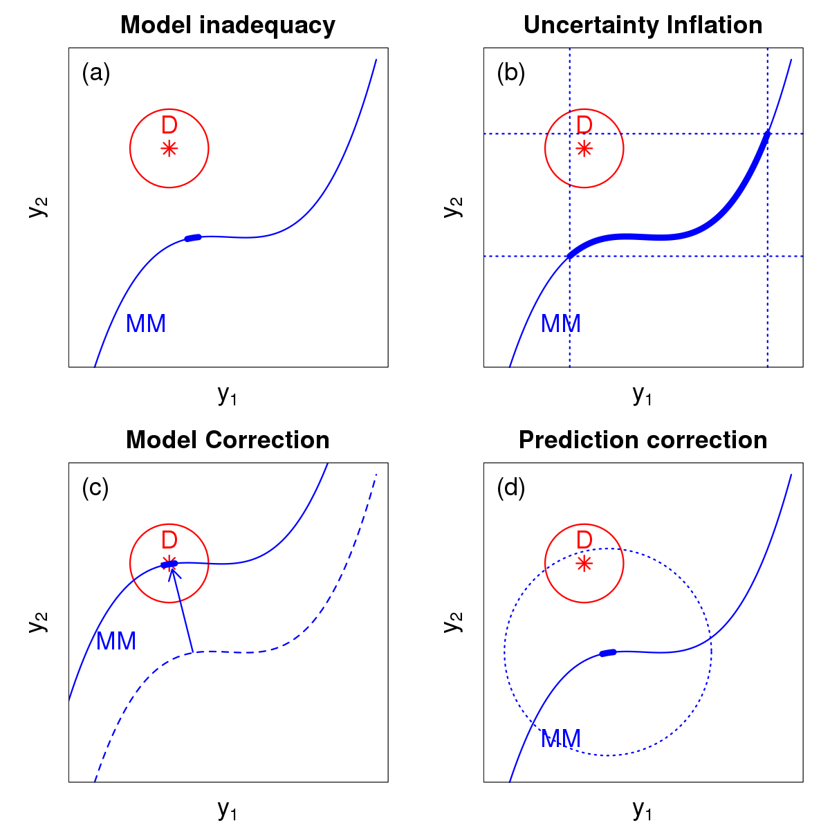
Figure 1: Schematic representation of model inadequacy and correction methods discussed in the text. A one-parameter model $M(x;\vartheta)$ is used to predict two values $y_{1}=M(x_{1};\vartheta)$ and $y_{2}=M(x_{2};\vartheta)$, to be compared with reference data represented by a point in data space, $D=\left\{d_{1}\pm u_{1},d_{2}\pm u_{2}\right\}$ (red star).
(a) Model inadequacy occurs when the point in the model manifold (MM, blue line) closest to $D$ (optimal parameter $\hat{\vartheta}\pm u_{\vartheta}$) does not intersect with a high probability volume around $D$ (red circle).
(b) Without change in the model, one defines a space of parameters values ($\boldsymbol{Q}=\left\{\vartheta_{min}\leq\vartheta\leq\vartheta_{max}\right\}$) which enables to reconcile model predictions with individual data : $d_{1}\in M(x_{1};\boldsymbol{Q})$ and $d_{2}\in M(x_{2};\boldsymbol{Q})$ (PUI; Sect. 3.3.2).
(c) The model can be corrected $M^{\prime}=M+\delta M$ to remove inadequacy (method GP; Sect. 3.3.1.1).
(d) Model predictions can be statistically corrected to be compatible with the data (method Disp; Sect. 3.3.1.2).

Considering the structure of the problem, accounting for model errors can be done along two directions, as depicted in Fig. 1 and summarized in Table 2:

1. out of the model manifold, by adding a correction term, which might either reduce the errors (GP; Fig. 1(c)), or represent them statistically (Disp; Fig. 1(d)); and

2. within the model manifold, by increasing the MPU by adapting the covariance matrix of its parameters (Fig. 1(b)). In order to do this, one has to replace the $N$-dimensional problem by a less-constrained one, such as $N$ one-dimensional problems (Margin) or a statistics-matching problem (ABC). One can also build a hierarchical model on data series designed along the control space (HierC).

Type		Action		Acronym		Section
Out of MM		Optimize dispersion parameter		Disp		3.3.1.2
		Optimize discrepancy function		GP		3.3.1.1
Within MM		Parameter uncertainty inflation
		a/ Target prediction uncertainty
		a.1/ Reweigh data (tweak $\boldsymbol{V}_{D}$)		VarInf		3.3.2.1
		a.2/ Optimize $\boldsymbol{V}_{\vartheta_{M}}$
		a.2.i/ $N$ 1D problems		Margin		3.3.2.2.1
		a.2.ii/ Statistics matching		ABC		3.3.2.2.2
		b/ Optimize local parameters		HierC		3.3.2.2.3

Table 2: Methods to handle model inadequacy.

3.3.1 Model correction out of the model manifold

3.3.1.1 GP: gaussian process.

The model inadequacy can be treated by adding a correction term (the so-called discrepancy function, $\delta M$) to the original model:

$$y_{i} =M(x_{i};\boldsymbol{\vartheta}_{M})+\delta M(x_{i};\boldsymbol{\vartheta}_{K})+\epsilon_{i}$$ (30)

$$R_{i} =y_{i}-M(x_{i};\boldsymbol{\vartheta}_{M})-\delta M(x_{i};\boldsymbol{\vartheta}_{K})$$ (31)

This approach is subject to parameter identification problems if the parameters of $M$ and $\delta M$ are optimized simultaneously without strong prior information [63, 43, 64]: $\delta M$ can in principle correct any error due to misspecification of $M$, which relaxes too strongly the constraints of the calibration data on $\boldsymbol{\vartheta}_{M}$.

The solution adopted in the present study is to constrain $\boldsymbol{\vartheta}_{M}$ with the posterior pdf resulting from an independent calibration of $M$. In this case, $\delta M(.)$ is designed to fit the residuals of $M(x;\boldsymbol{\vartheta}_{M})$ by a Gaussian Process (GP) [65, 47] of mean $0$ and covariance matrix

$$V_{M,ij} =\rho(x_{i},x_{j}),$$ (32)

based on a Gaussian kernel

$$\rho(u,v)=\alpha^{2}\exp(-\beta^{2}(u-v)^{2}).$$ (33)

Both parameters $\alpha$ and $\beta$ have to be estimated in addition to $\boldsymbol{\vartheta}_{M}$.

The predictive posterior pdf can be derived in closed form expression

$$p_{M}(\tilde{y}|\tilde{x},\boldsymbol{D})=\mathcal{N}(\boldsymbol{\Omega}^{T}\boldsymbol{V}^{-1}\boldsymbol{y},\alpha^{2}-\boldsymbol{\Omega}^{T}\boldsymbol{V}^{-1}\boldsymbol{\Omega}),$$ (34)

where $\boldsymbol{\Omega}_{i}=\rho(x_{i},\tilde{x})$ and $\boldsymbol{V}$ is defined by Eq. 9.

3.3.1.2 Disp: dispersion parameter.

One might also consider a simpler correction by taking

$$\delta M(x_{i};\sigma) \sim \mathcal{N}(0,\sigma^{2})$$ (35)

$$V_{M,ij} = \sigma^{2}\delta(i-j)$$ (36)

This version of model correction does not suffer from the parameters identification problem of the GP approach. It is statistically justified if there is no visible trend in the residuals (model errors randomly distributed with respect to the control variable) [14], but it can also be useful if one is interested in quantifying a representative scale of model inadequacy without correcting it explicitly.

For predictions, the dispersion parameter $\sigma$ has to be used in Eq. 2, through the $f(\tilde{y}|\tilde{x},\boldsymbol{\vartheta}_{M})$ pdf. In this case, one has simply $f=\mathcal{N}(M(\tilde{x};\boldsymbol{\vartheta}_{M}),\sigma^{2})$.

3.3.2 Parameter uncertainty inflation

For deterministic models, the main source of prediction uncertainty is parameter uncertainty. In the calibration process, parameter uncertainty is a byproduct, but this can be transgressed by using it as a variable to adjust MPU. In effect, parameter uncertainty can be tuned in order to provide a prediction uncertainty $u_{M}$ which is large enough to represent model inadequacy. We call this approach parameter uncertainty inflation (PUI) [49]. As for the model correction approach, this leads to a stochastic model, albeit with an internal/embedded stochastic source [46], opening the door to calibration transferability.

Several approaches have been proposed in the computational chemistry literature: in one case, the covariance matrix $\boldsymbol{V}_{D}$ is scaled in order to produce suitable MPU (VarInf); in the other cases, the covariance matrix of the parameters $\boldsymbol{V}_{\vartheta_{M}}$ is directly optimized, a more complex option with several variants (Margin, ABC, HierC). Some of these PUI methods (VarInf, Margin & ABC) have been reviewed recently [49], and are presented here to ensure a self-contained framework.

3.3.2.1 VarInf: variance inflation.

Scaling of the data covariance matrix is a simple way to increase parameter uncertainty to a prescribed level. As discussed by Pernot [49], it has been used, for instance, in the calibration of the mBEEF density functional,[66, 67, 10] or, indirectly, in the estimation of the scaling factor uncertainty for ab initio properties statistical correction.[68, 69, 70]

An empirical likelihood is built by scaling the data covariance matrix

$$p(\boldsymbol{D}|\boldsymbol{\vartheta},T)\propto\left|T\boldsymbol{V}_{D}\right|^{-1/2}\exp\left(-\frac{1}{2T}\boldsymbol{R}^{T}\boldsymbol{V}_{D}^{-1}\boldsymbol{R}\right),$$ (37)

with a scaling factor $T$ to be determined.

Optimization of $T$ using this likelihood leads to the Birge ratio procedure used in metrological inter-laboratory comparisons to reconcile inconsistent data.[71, 55, 72] Assuming an adequate model and misestimated data variances, this approach rescales the data variances in order to get a valid statistical estimation of the weighted data mean. In practice, $T$ is chosen so as to provide a unit Birge ratio with Eq. 37, i.e., $T=R_{B}^{0}$, where

$$R_{B}^{0}=\frac{1}{N-\nu}\boldsymbol{\hat{R}}^{T}\boldsymbol{V}_{D}^{-1}\boldsymbol{\hat{R}}.$$ (38)

In the hypothesis of reliable data variances considered here, $T$ is chosen to compensate for model inadequacy and obtain valid prediction statistics:

• In the ensemble method,[66, 67, 10] $T$ is chosen using a statistical mechanics analogy with a temperature, leading to[49]

  $$T =\frac{N-\nu}{\nu}\,R_{B}^{0}.$$ (39)

  This approach is called VarInf_Rb in the following.

• Assuming a near-linear dependence of the model on its parameters in their uncertainty range, an alternative estimation of $T$ can be based on Eq. 4, in such a way that the mean variance of model predictions reproduces the mean squared residuals [13]. In the presence of non-negligible measurement uncertainty, one has

  $$T\simeq\frac{MSR-\overline{u^{2}}}{MPV^{0}-\overline{u^{2}}},$$ (40)

  using the mean prediction variance $MPV^{0}$ from a reference calibration with $T=1$, and $\overline{u^{2}}=\sum_{i}u_{i}^{2}/N$. This approach is called VarInf_MSR in the following.

In all cases, prediction is done with Eq. 2.

3.3.2.2 Parameters covariance.

In the direct approach, the model’s parameters are considered as random variables, with a pdf conditioned by a set of hyperparameters, typically their mean values $\boldsymbol{\mu}_{\vartheta}$ and a covariance matrix $\boldsymbol{V}_{\vartheta}$, defining a multivariate normal distribution $p(\boldsymbol{\vartheta}_{M}|\boldsymbol{\mu}_{\vartheta_{M}},\boldsymbol{V}_{\vartheta_{M}})$.

Such stochastic parameters can be handled in the bayesian inference problem, either at the model level, leading to a stochastic model within the standard likelihood framework (Eq. 8), or at the likelihood level. An indirect way to estimate $p(\boldsymbol{\vartheta}_{M}|\boldsymbol{\mu}_{\vartheta_{M}},\boldsymbol{V}_{\vartheta_{M}})$ is to use a hierarchical model with local sets of parameters $\boldsymbol{\vartheta}_{M}^{(\kappa_{i})}$ to represent complementary sections of the control parameter space (HierC) [9].

3.3.2.2.1 Margin: Model level.

At the model level, one estimates the impact of stochastic parameters on model predictions by uncertainty propagation[34]

$$f_{M}(\boldsymbol{\xi};\boldsymbol{x},\boldsymbol{\mu}_{\vartheta_{M}},\boldsymbol{V}_{\vartheta_{M}})=\int\thinspace\prod_{i=1}^{N}\delta\left(\xi_{i}-M(x_{i};\boldsymbol{\vartheta}_{M})\right)\,p(\boldsymbol{\vartheta}_{M}|\boldsymbol{\mu}_{\vartheta_{M}},\boldsymbol{V}_{\vartheta_{M}})\,d\boldsymbol{\vartheta}_{M},$$ (41)

where $f_{M}(.;\boldsymbol{x},\boldsymbol{\mu}_{\vartheta_{M}},\boldsymbol{V}_{\vartheta_{M}})$ is the multivariate pdf of the model’s predictions at the vector of control points $\boldsymbol{x}$.

Inserting the resulting stochastic model in Eq. 8 can be done by replacing $M(x_{i};\boldsymbol{\vartheta}_{M})$ by the mean predictions (Eq. 3) and their covariance matrix $\boldsymbol{V}_{M}$

$$p(\boldsymbol{D}|\boldsymbol{\mu}_{\vartheta_{M}},\boldsymbol{V}_{\vartheta_{M}},\boldsymbol{\vartheta}_{V})\propto\left|\boldsymbol{V}_{D}+\boldsymbol{V}_{M}\right|^{-1/2}\exp\left(-\frac{1}{2}\boldsymbol{R}^{T}\left(\boldsymbol{V}_{D}+\boldsymbol{V}_{M}\right)^{-1}\boldsymbol{R}\right),$$ (42)

where

$$\boldsymbol{V}_{M,ij} \equiv u_{M}^{2}(x_{i},x_{j})=\boldsymbol{J}^{T}(x_{i};\boldsymbol{\mu}_{\vartheta_{M}})\boldsymbol{V}_{\vartheta_{M}}\boldsymbol{J}(x_{j};\boldsymbol{\mu}_{\vartheta_{M}}),$$ (43)

$$R_{i} =y_{i}-\mu_{M|D}(x_{i}).$$ (44)

Note that using the full variance matrix of Eq. 42 in the calculation of the Birge ratio (Eq. 13) should enable to validate the model with $R_{B}\simeq 1$ by increasing the variance without affecting the residuals.

For a deterministic model $M$, when the number of parameters is smaller than the number of data points, $\boldsymbol{V}_{M}$ is singular (non positive-definite), causing the likelihood to be degenerate, and the calibration to be intractable [46]. By definition, for inadequate models, the data covariance matrix is numerically too small to alleviate the degeneracy problem. As all data points cannot be reproduced simultaneously by the model (Fig. 1(b)), one has to replace the multivariate problem by a set of univariate problems (marginal likelihoods [46, 30]), i.e., one ignores the covariance structure of model predictions by taking

$$\boldsymbol{V}_{M,ij}=u_{M}^{2}(x_{i},x_{j})\delta(i-j).$$ (45)

3.3.2.2.2 ABC: Likelihood level.

A new likelihood, conditioned on the hyperparameters to be inferred,[48, 46] is obtained by integration of the standard likelihood (Eq. 8) over the possible values of the parameters (marginalization)

$$p(\boldsymbol{D}|\boldsymbol{\mu}_{\vartheta_{M}},\boldsymbol{V}_{\vartheta_{M}},\boldsymbol{\vartheta}_{V})=\int p(\boldsymbol{D}|\boldsymbol{\vartheta}_{M},\boldsymbol{\vartheta}_{V})p(\boldsymbol{\vartheta}_{M}|\boldsymbol{\mu}_{\vartheta_{M}},\boldsymbol{V}_{\vartheta_{M}})\,d\boldsymbol{\vartheta}_{M}.$$ (46)

As in the previous case, it is pointed out by Sargsyan et al.[46] that this likelihood is in general degenerate, so that the inference problem has to be solved by alternative methods, such as Approximate Bayesian Computation (ABC).[73, 74] In this case, the full likelihood (Eq. 46) is replaced by a tractable expression, based on summary statistics of the model predictions, to be compared with similar statistics of the data. An example is provided in Sargsyan et al.,[46] where the mean value of the model and its prediction uncertainty are used. A version adapted to the present problem, with an explicit treatment of experimental uncertainty is used here:

$$p_{ABC}(\boldsymbol{D}|\boldsymbol{\mu}_{\vartheta_{M}},\boldsymbol{V}_{\vartheta_{M}},\boldsymbol{\vartheta}_{V})\propto\exp\left(-\frac{1}{2}\boldsymbol{R}^{T}\boldsymbol{V}_{D}^{-1}\boldsymbol{R}\right)\times p_{reg}(\boldsymbol{D}|\boldsymbol{\mu}_{\vartheta_{M}},\boldsymbol{V}_{\vartheta_{M}})$$ (47)

where the first term has the same expression as the standard likelihood (Eq. 8) using residuals evaluated at the mean of the model prediction, and the second term ensures that the predicted model uncertainty $u_{M}(x_{i})$, combined with experimental uncertainty $u_{i}$, is of a magnitude compatible with the residuals

$$p_{reg}(\boldsymbol{D}|\boldsymbol{\mu}_{\vartheta_{M}},\boldsymbol{V}_{\vartheta_{M}})=\exp\left(-\sum_{i=1}^{N}\frac{\left(\sqrt{u_{M}^{2}(x_{i})+u_{i}^{2}}-|R_{i}|\right){}^{2}}{2u_{i}^{2}}\right).$$ (48)

As evidenced in our notation, this term can also be seen as a regularization function, necessary to constrain the parameters covariance matrix $\boldsymbol{V}_{\vartheta_{M}}$ in the inference process. The constraint imposed here is a statistical variant of Eq. 16.

3.3.2.2.3 HierC: local parameters in control space

Model inadequacy can sometimes be seen as a consequence of the use of a unique parameter set in different experimental conditions: a “better” model can indeed be obtained by using different values of the parameters along the control space. This can be achieved by modeling the dependence of the physical parameters on the control variable [75, 76, 77], or by splitting the data in series along the control space and using a hierarchical model identical to the one in Section 3.2.2.2 for inference of the hyperparameters describing the model’s parameters distribution (model $\mathcal{M}_{H2}$ in Wu et al. [9]). To differentiate both hierarchical schemes, the present one is named HierC.

3.4 Combined methods

Dealing with systematic measurement errors and model inadequacy errors requires to combine the methods exposed above. Combined methods are noted by joining the acronyms of the components, e.g. GP-Shift, Hier-Cov…

Not all combinations are favorable: for methods like GP and ABC, which rely on a good estimation of model inadequacy residuals, the explicit correction of systematic measurement errors by the Shift method is the most coherent option.

The Hier method can accommodate the Shift and Cov approaches, but care has to be taken with identification issues between shift and model parameters. This will be illustrated in Section 4.2.3.

4 Applications

Before applying the statistical calibration/prediction models exposed above to reference data, we adopt a step-wise approach on synthetic data to illustrate their advantages and drawbacks. The synthetic data are designed to mimic the main features of a dataset of temperature-dependent measurements of Krypton viscosity.

4.1 Viscosity model

The following Chapman-Enskog model provides the viscosity $\eta$ in $\mu$Pa.s [3], when the inputs are in K ($T$ and $\epsilon_{LJ}$) and Å ($\sigma_{LJ}$):

$$\eta = M(T;\epsilon_{LJ},\sigma_{LJ})=2.6693\frac{\sqrt{mT}}{\sigma_{LJ}^{2}\Omega}$$ (49)

$$\Omega = \frac{A}{(T^{*})^{B}}+\frac{C}{\exp(DT^{*})}+\frac{E}{\exp(FT^{*})}$$ (50)

with $T^{*}=T/\epsilon_{LJ}$, $m=83.978$ g/mol, the molar mass of Kr, and dimensionless coefficients $A=1.16145$, $B=0.14874$, $C=0.52487$, $D=0.77320$, $E=2.16178$, and $F=2.43787$.

4.2 Synthetic data

Synthetic data are generated by random sampling of systematic errors, $s$, and random errors, $\epsilon$, in the generative model

$$y_{i}=M(x_{i};\boldsymbol{\vartheta}_{0})+s^{(\kappa_{i})}+\epsilon_{i}$$ (51)

with reference LJ parameters $\boldsymbol{\vartheta}_{0}=\left\{\epsilon_{LJ}:\thinspace 195\,\textrm{K},\thinspace\sigma_{LJ}:\thinspace 3.6\,\text{\AA}\right\}$.

Random errors are modeled as an additive heteroscedastic noise

$$\epsilon_{i}\sim\mathcal{N}(0,f_{i}\times y_{i}),$$ (52)

with uncertainty factor

$$f_{i}=f_{0}*\exp\left(g\left|\frac{1}{x_{i}}-\frac{1}{300}\right|\right)$$ (53)

where $f_{0}=0.001$ and $g=50$ K. This functional shape enforces that the relative measurement uncertainties are smaller at room temperature.

Systematic errors are generated from a normal distribution of mean $0$ and standard deviation to be specified.

As the generative model for experimental uncertainty is unknown in the analysis of experimental data, one has to build an approximation for prediction of experimental data. In the following, one uses the mean relative uncertainty calculated on the calibration dataset $\overline{u}_{r}=1/N\sum u_{i}/y_{i}$, multiply it by the model value at the prediction point and ensures that the result does not get below the minimal experimental uncertainty in the dataset, $u_{min}$:

$$p(\tilde{y_{e}}|\tilde{y})=\mathcal{N}(\tilde{y},\mathrm{max}(u_{min},\,\tilde{y}\times\overline{u}_{r})).$$ (54)

4.2.1 SD-1: model inadequacy

A first dataset of size $N=100$ is generated by simulating 10 series of data with cardinals between 5 and 15 and with overlapping temperature ranges. The control points $x_{i}$ are located between $T=120$ and $2000$ K. The series are consistent, i.e. $s^{(\kappa_{i})}=0$ in the generative model, Eq. 51. The standard deviation of the random noise in this set is about $0.07$ $\mu$Pa.s.

To simulate model inadequacy, one uses for data analysis a modified version of the Chapman-Enskog model (Section 4.1), in which the constant $C$ was replaced by $C^{\prime}=C*0.5$. The standard deviation from the true model due to this perturbation before model calibration is $0.55$ $\mu$Pa.s.

The following statistical models were run on the SD-1 dataset:

• Std, with parameters $\epsilon_{LJ}$, $\sigma_{LJ}$ and $\sigma$;

• Disp, with the same parameters (different interpretation for $\sigma$);

• GP, with parameters $\epsilon_{LJ}$, $\sigma_{LJ}$, $\alpha$ and $\beta$ – in order to prevent identification problems, the posterior pdf of the “Disp” model is used as prior for $\epsilon_{LJ}$ and $\sigma_{LJ}$;

• WLS, with parameters $\epsilon_{LJ}$, $\sigma_{LJ}$;

• VarInf_Rb and VarInf_MSR, with prescribed value of $T$ (Eq. 39 and Eq. 40, respectively) and parameters $\epsilon_{LJ}$, $\sigma_{LJ}$;

• Margin and ABC, with parameters $\epsilon_{LJ}$, $\sigma_{LJ}$, $u_{\epsilon}$, $u_{\sigma}$ and $\rho$, such as

  $$\boldsymbol{V}_{\vartheta_{M}}=\left(\begin{array}[]{cc}u_{\epsilon}^{2}&u_{\epsilon}u_{\sigma}\rho\\ u_{\epsilon}u_{\sigma}\rho&u_{\sigma}^{2}\end{array}\right).$$ (55)

  The validity of the linear approximation for the estimation of model uncertainty in the Margin and ABC methods has been checked by calculating the relative error of a linear approximation of the model over the whole range of temperature and a sample of LJ parameters drawn from the posterior pdf (1000 points). The maximal relative error is about $10^{-4}$, validating the linear approximation.

• HierC, based on a serialization of the dataset along the control variable, with parameters $\epsilon_{LJ}$, $\sigma_{LJ}$, $u_{\epsilon}$, $u_{\sigma}$, $\rho$ and $\sigma$. The data were arbitrarily split into $5$ series at $T=300$, $600$, $900$ and $1200$ K.

A summary of the parameters of all models is reported in Table (3). The residuals at the MAP for all methods and the prediction bands are plotted in Fig. 2, and the summaries of the posterior samples of the LJ parameters are shown in Fig. 3.

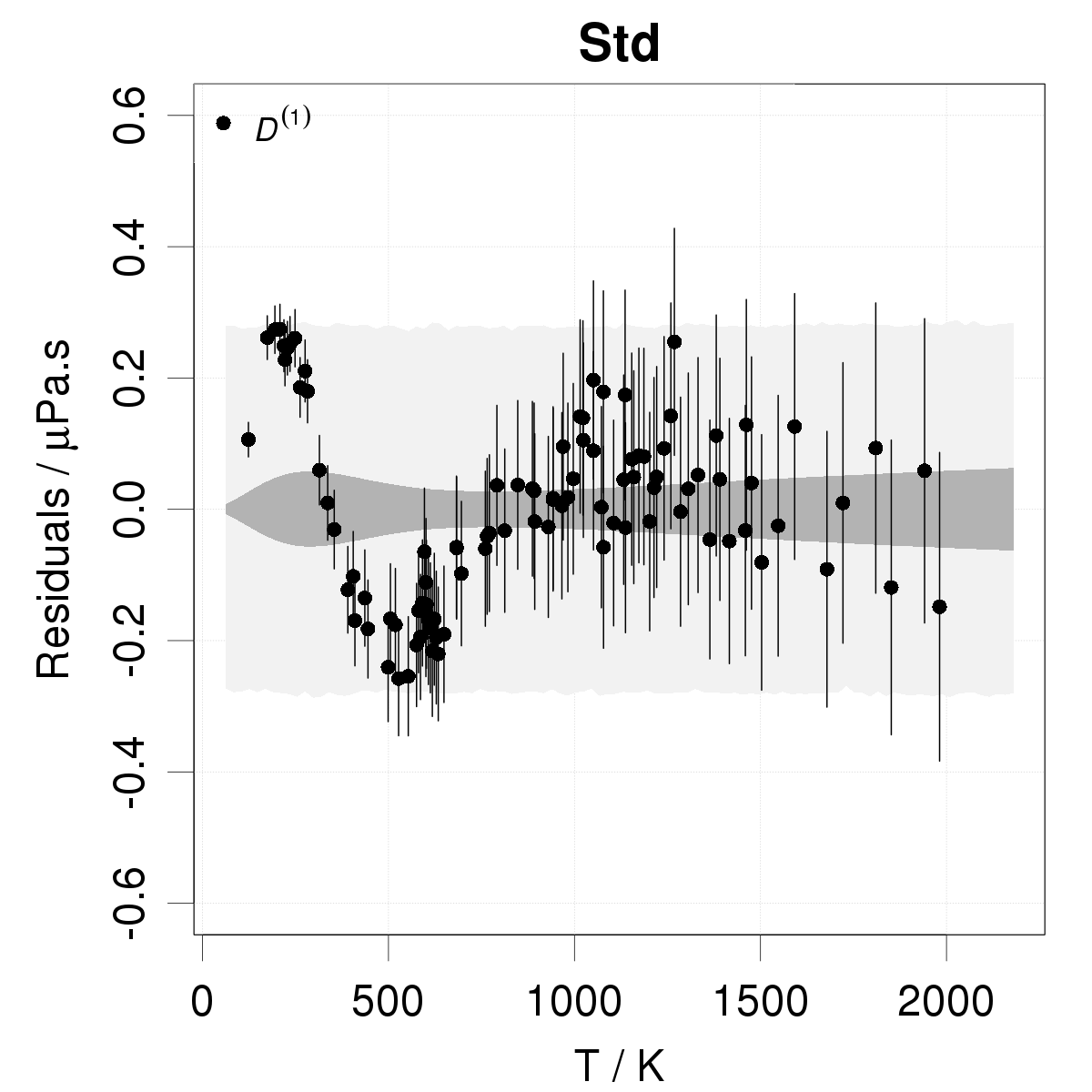
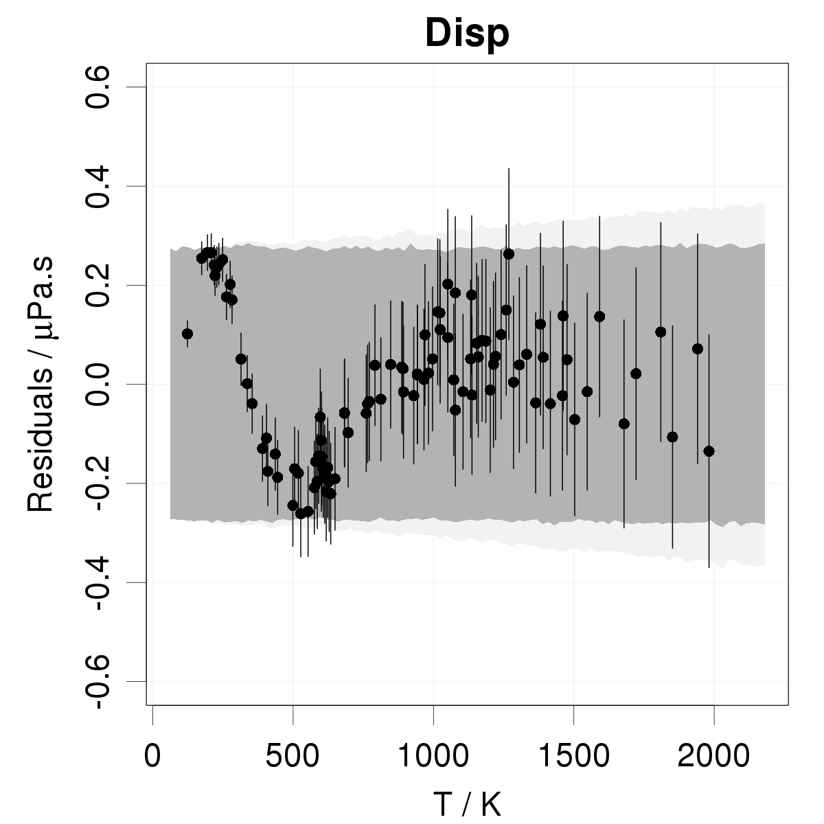
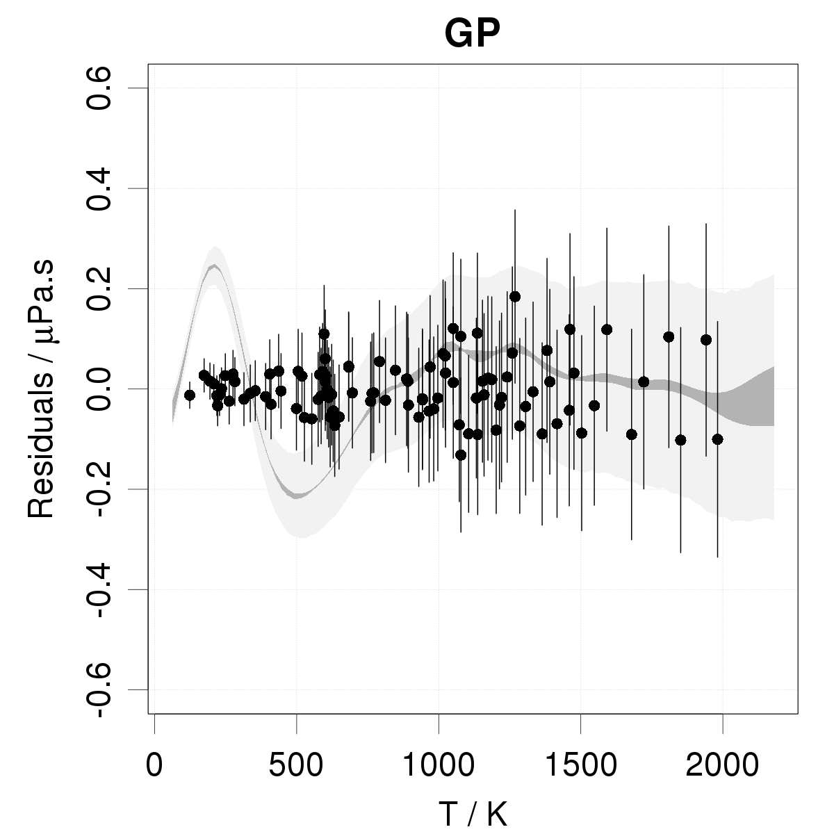
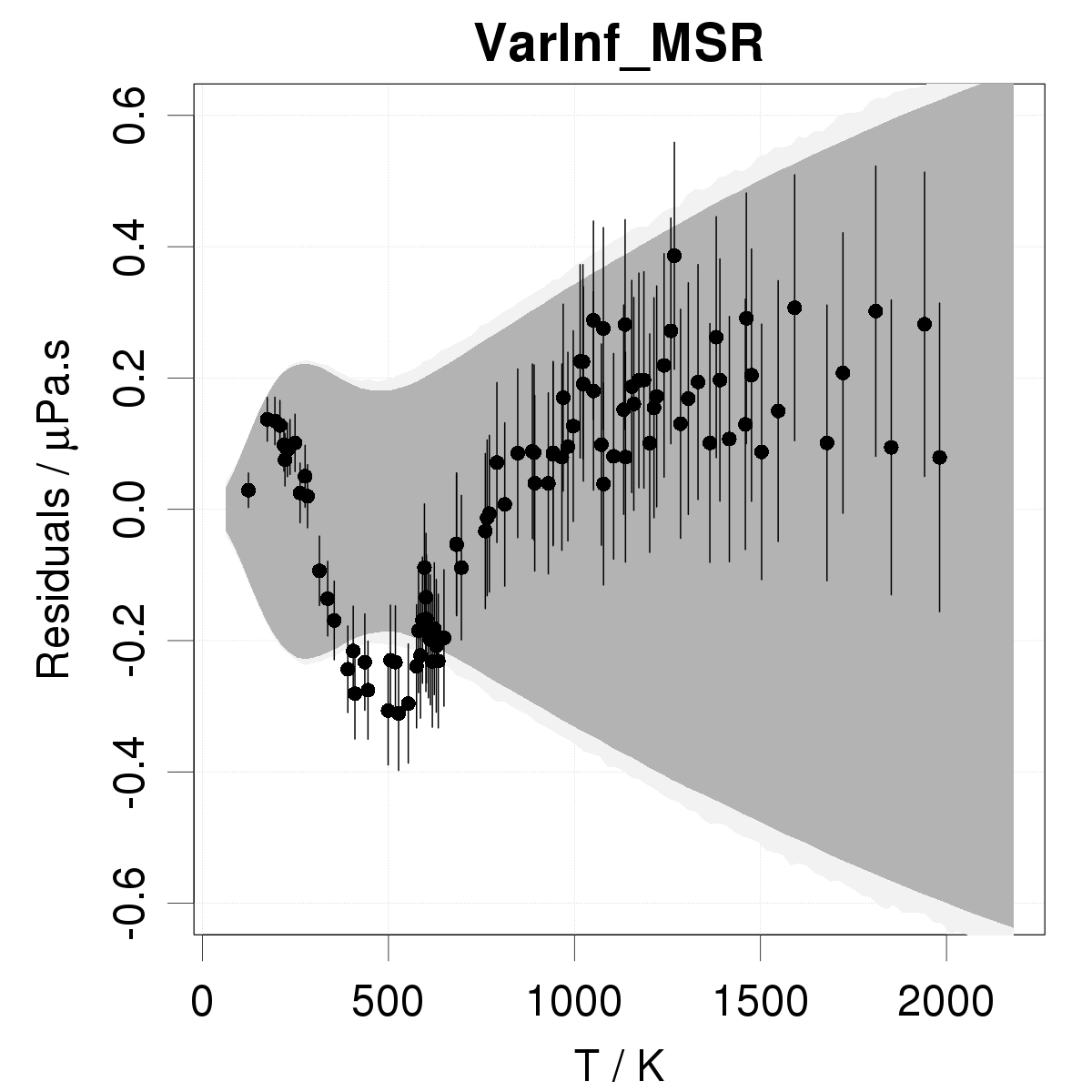
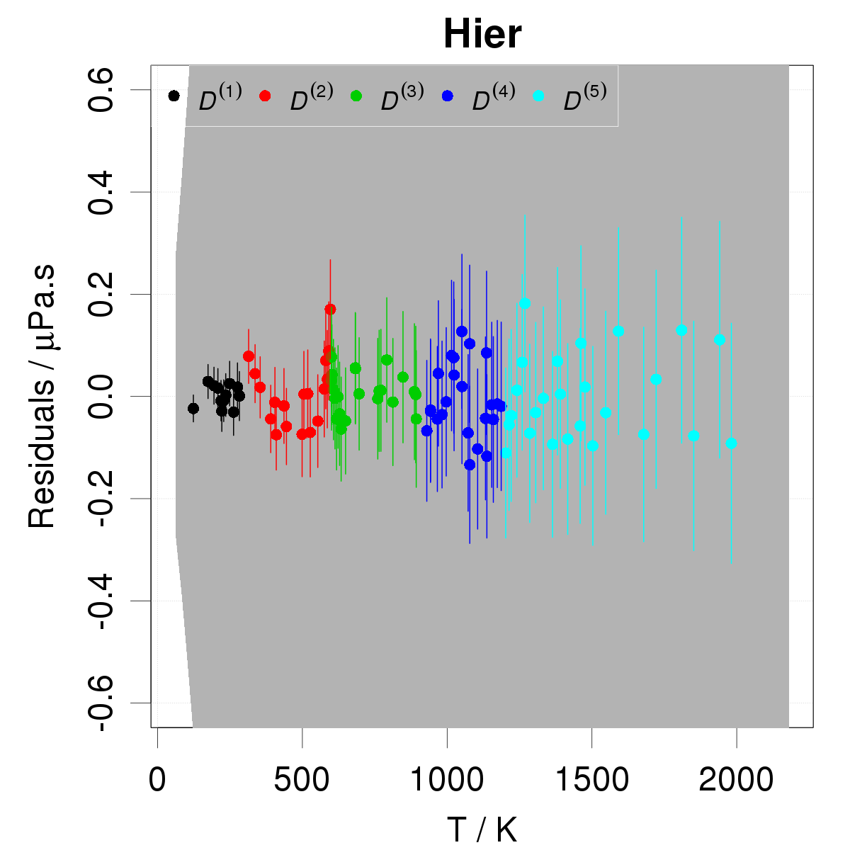
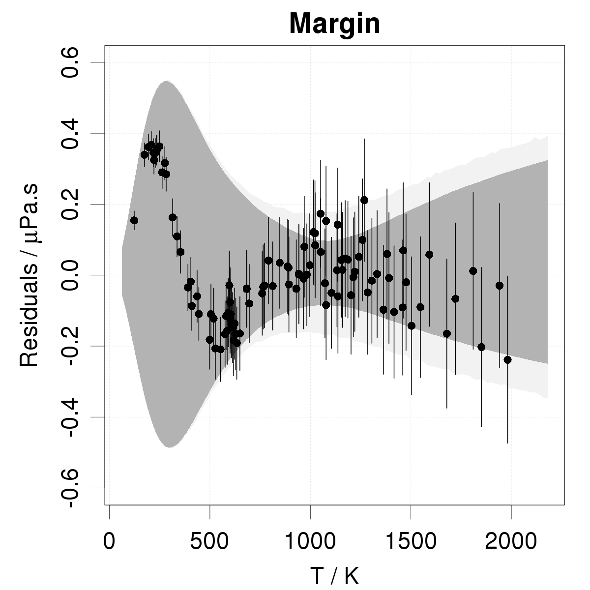
Figure 2: Calibration residuals and posterior prediction intervals for data SD-1. For each model, the results are centered on the maximum a posteriori results (MAP). The dark gray band represents the model prediction 95 % probability interval ($p_{M}$) and the light gray area the experiment prediction 95 % probability interval ($p_{e}$).

The structure and serial correlation of the residuals of the Std method reveal the amplitude and shape of model inadequacy after calibration (Fig. 2). The $RMSD$ of $0.14$ $\mu$Pa.s shows that parameter optimization is able to correct a large fraction of the original inadequacy ($0.55$ $\mu$Pa.s). This is done however at the expense of a large bias in parameters recovery, as can be seen in Table 3 and Fig. 3.

Only two models are able to improve over the $RMSD$ of the Std method and recover the level of random experimental noise ($0.07$ $\mu$Pa.s): the gaussian process GP, which completes the model with an adapted correction term, and the hierarchical model HierC, which uses local LJ parameters adapted for different temperature zones. The WLS, VarInf-type and ABC methods achieve slightly higher $RMSD$ ($0.18$ $\mu$Pa.s). The first ones have one less parameters than the Std method. In the case of the ABC method, this is due to the additional constraint in the likelihood.

Several methods have Birge ratio differing notably from the unit value: WLS ($R_{B}=13.0$) has no provision to compensate for model inadequacy; ABC ($1.3$) for the same reason as above; GP ($0.87$) might present some level of overfitting; and the VarInf-type methods ($0.02-0.03$) are based on exalted data variance. It is not possible to validate the latter methods by such statistics at the calibration level.

Model		$\epsilon_{LJ}$		$\sigma_{LJ}$			$\sigma$			$MR$			$RMSD$		$R_{B}$			$u_{e|D}$
		(K)		(Å)			($\mu$Pa.s)			($\mu$Pa.s)			($\mu$Pa.s)					($\mu$Pa.s)
Ref		195		3.	6										1.	0
Std		254(1)		3.	527(2)		0.	14(1)		0.	00		0.14		1.	0		0.	14
Disp		254(1)		3.	528(2)		0.	14(1)		0.	00		0.14		0.	94		0.	16
GP		253(1)		3.	529(2)		-			0.	00		0.06		0.	87		0.	07
WLS		247.0(2)		3.	5391(5)		-			0.	03		0.18		13.	0		0.	07
VarInf_Rb∗		247(6)		3.	54(1)		-			0.	03		0.18		0.	02		0.	23
VarInf_MSR∗		247(5)		3.	54(1)		-			0.	03		0.17		0.	02		0.	18
Margin		258(2)		3.	522(2)		-			0.	01		0.15		0.	91		0.	15
$u_{\epsilon},\,u_{\sigma}$		10(1)		0.	012(2)
$\rho$		-0.997(3)
ABC		247.5(2)		3.	5389(4)		-			0.	06		0.18		1.	3		0.	17
$u_{\epsilon},\,u_{\sigma}$		3.0(2)		0.	0007(6)
$\rho$		0.2(5)
Hier		251(10)		3.	54(2)		0.	02(1)		0.	00		0.06		1.	1		1.	20
$u_{\epsilon},\,u_{\sigma}$		19(9)		0.	04(2)
$\rho$		-0.7(3)

Table 3: Summary of the main parameters and statistics for the methods tested on the SD-1 set. The first line (labeled Ref) provides reference value of the parameters and statistics.
^∗ The scale factors $T$ for VarInf_MSR and VarInf_Rb are respectively 435 and 643.

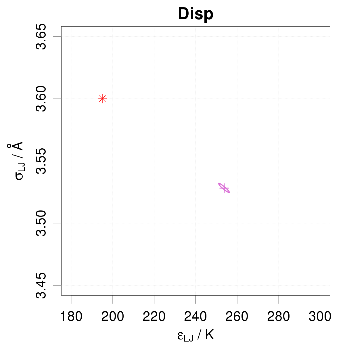
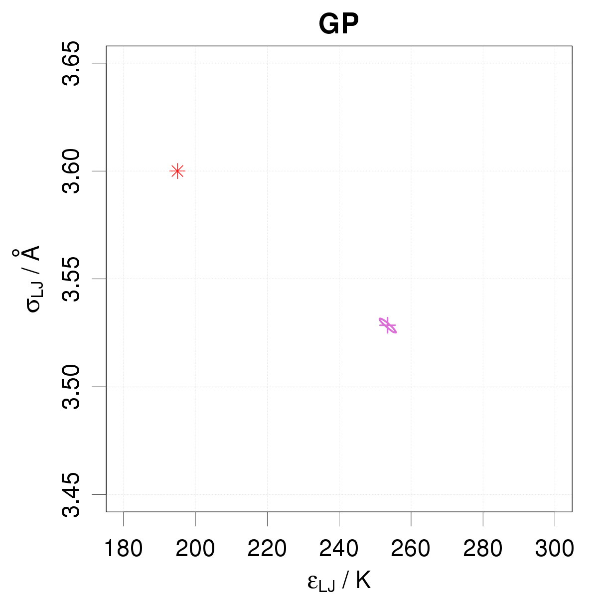
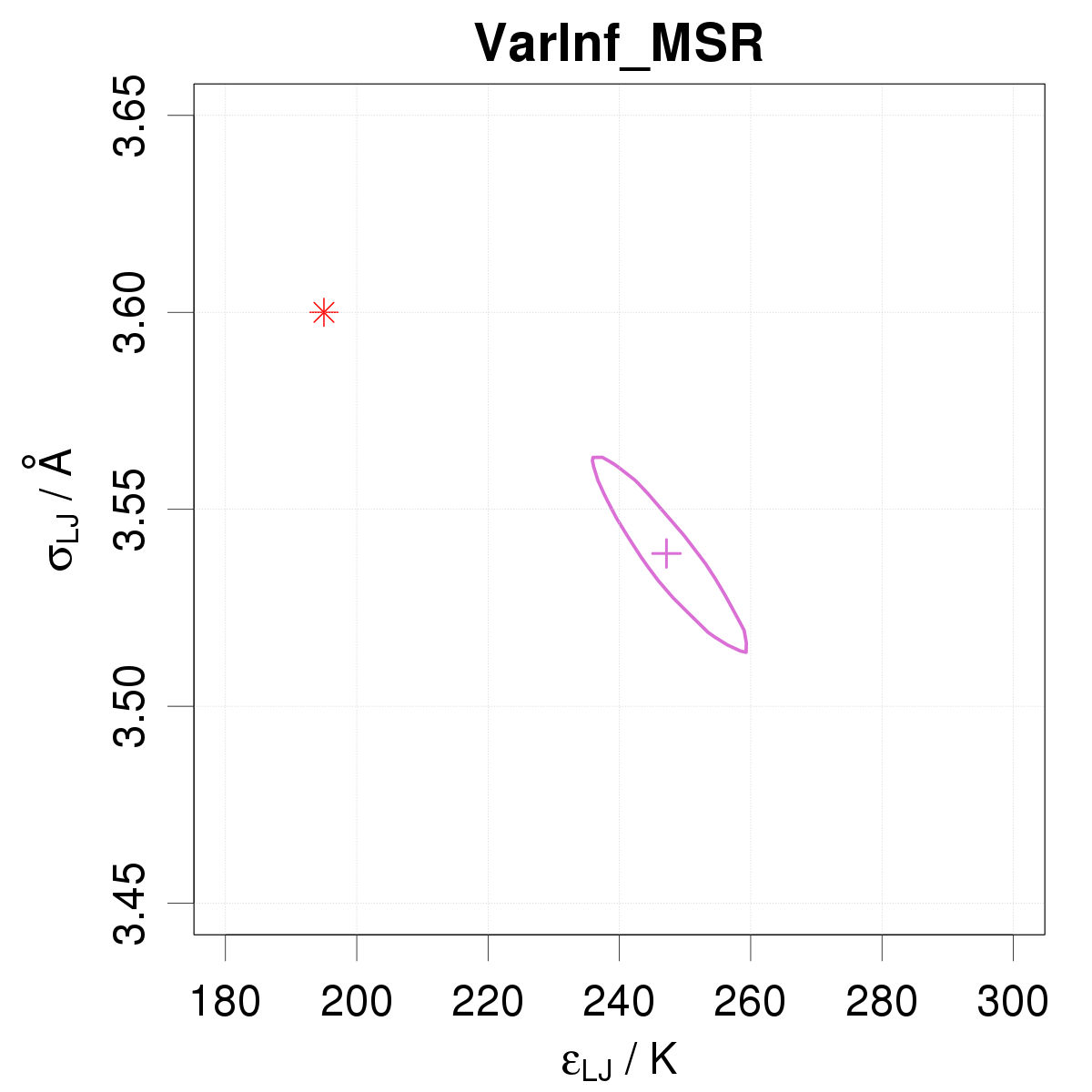
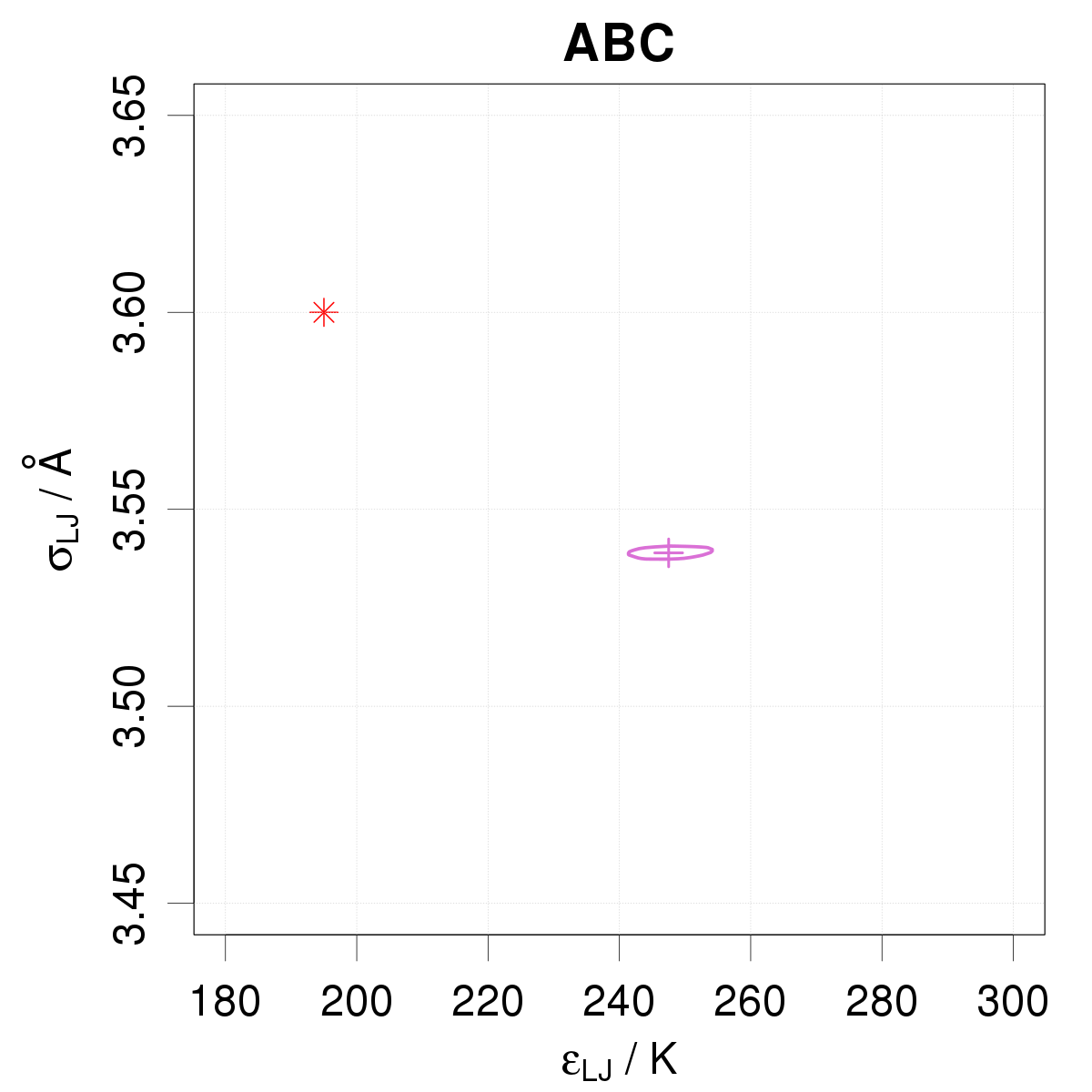
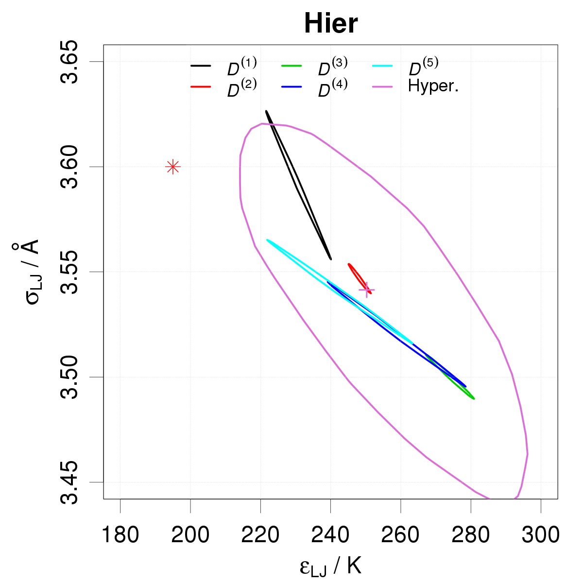
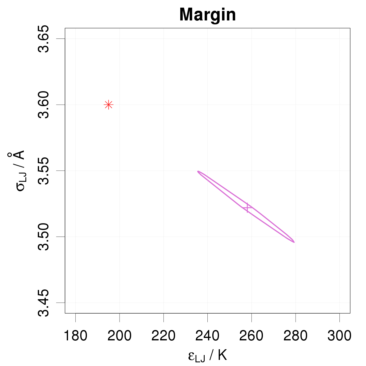
Figure 3: Posterior samples of LJ parameters calibrated on data SD-1: the contours represent 95 % probability intervals; the red cross depicts the reference value of the parameters.

The posterior samples show large differences (Table 3 and Fig. 3). The Std and Disp models have similar outputs, the main difference lying in the signification attributed to the residual dispersion parameter $\sigma$. In the Disp method, $\sigma$ is part of the model, and therefore contributes to MPU, which ensures that the model prediction band covers correctly the part of the residuals due to model systematic errors (Fig. 2).

The posterior pdf of the GP method for the LJ parameters is identical to its prior pdf which was taken from the Disp posterior pdf. This constraint is intended to solve the parameters identifiability problem of this approach.

Methods based on the PUI strategy (VarInf-type, Margin, ABC) display larger dispersion of the LJ parameters, while the Hier method produces the posterior sample with the largest dispersion.

Considering the prediction statistics $u_{e|D}$, it is close to the $RMSD$ for all methods, except: WLS, for the same reasons as above; VarInf_Rb, which has overestimated parameter uncertainty; and Hier, which has a strongly over-estimated prediction uncertainty, due to the large dispersion of the LJ parameters necessary to their adaptation to the full temperature range.

The impact of the posterior samples on the predictions is observable in Fig. 2. In the present scenario, one expects that the model prediction confidence band (from distribution $p_{M}$, Eq. 2) accounts for model inadequacy. The Std model cannot be successful because of the ambiguity on the meaning of parameter $\sigma$. This ambiguity is solved in Disp, as this parameters enters the stochastic part of the model describing model errors. In this case, the prediction confidence band has a constant width over the control parameter range and covers correctly model inadequacy.

By construction, the GP model has prediction bands which follow perfectly the structure of model inadequacy. In contrast, the Hier model, which achieved also very good residuals, has strongly over-estimated prediction bands.

Among the remaining PUI methods, VarInf_MSR and Margin have prediction bands which cover well the residuals, but with a structure which does not correlate well with model inadequacy. The ABC method presents more regular prediction bands.

Note that Pernot[49] observed a multimodality in the posterior pdf of the hyperparameters for the Margin and ABC distribution on a similar problem. Each mode corresponded to a minimal or near-minimal value for the $u_{\epsilon}$, $u_{\sigma}$ and $\rho$ hyperparameters. In the present case, no multimodality is observed, but the posterior pdf for Margin is localized at a VarInf-like solution corresponding to $\rho\simeq-1$ (Table 3 and Fig. 3), whereas the ABC method adopts a mode where $u_{\sigma}$ is very small.

Considering the results of this test, the methods best adapted to quantify model inadequacy errors would be Disp, GP and ABC.

4.2.2 SD-2: data inconsistency

The SD-2 dataset of size $N=100$ is generated by simulating 10 series of data with cardinals between 5 and 15, shifted by a random factor $s^{(\kappa_{i})}\sim\mathcal{N}(0,0.5)$, and with overlapping temperature ranges. The standard deviation of the random noise in this set is about $0.06$ $\mu$Pa.s, and the systematic errors contribute for $0.42$ $\mu$Pa.s.

There is no model inadequacy in this scenario, so the relevant models are:

• a variant of Disp, with parameters $\epsilon_{LJ}$, $\sigma_{LJ}$ and $\tau$, the latter describing inter-series dispersion instead of model inadequacy;

• Shift, where the serial shifts are treated explicitly as realizations of a random process with dispersion $\tau$ (hierarchical model);

• Cov, with parameters $\epsilon_{LJ}$, $\sigma_{LJ}$ and $\tau$;

• Hier, a hierarchical model with parameters $\epsilon_{LJ}$, $\sigma_{LJ}$, $u_{\epsilon}$, $u_{\sigma}$, and $\rho$, as proposed by Wu et al. [9] ($\mathcal{M}_{H1}$ model), and in which the LJ parameters are expected to compensate for systematic measurement errors; and

• Hier-Shift and Hier-Cov, combinations of the Hier model and the Shift and Cov descriptions of systematic data errors. These combined model are used here to show the interplay of model parameters and experimental systematic errors.

All methods recover correctly the reference LJ parameters (Table 4, Figs 4 & 5). The Shift, Hier and Hier-Shift models are able to efficiently correct the systematic errors and produce very small residuals, comparable with the random errors ($RMSD=0.06$ $\mu$Pa.s). The other methods reach a level compatible with the systematic errors ($RMSD\sim 0.4$ $\mu$Pa.s). Similarly, all methods reach adequate values of $R_{B}$.

When comparing the posterior pdfs of the parameters (Fig. 5), it is striking that models accounting explicitly for data inconsistency achieve smaller parameter uncertainty (e.g., Shift vs. Disp or Hier-Shift vs. Hier). In the Disp case, the hypothesis of independent data unduly increases parameter uncertainty. When the covariance structure of the data is taken into account (model Hier-Cov), the hierarchical model does not attempt to adapt the LJ parameters to compensate for experimental systematic errors and provides a much more concentrated posterior sample (Fig. 5).

For the Hier method, the mean prediction error $u_{e|D}$ ($0.5$ $\mu$Pa.s) is considerably larger than the $RMSD$ ($0.06$ $\mu$Pa.s), which is due to the choice of absorbing systematic experimental errors into the parameters. It is also the method with the largest prediction bands. The Hier-Shift method has also an excess of prediction uncertainty, although at a lesser level.

Fig. 6 shows that the Shift and Hier-Shift methods are able to recover correctly the shifts used to generate the data. However, due to the interactions with the local LJ-parameters, the uncertainties on the recovered shifts are much larger in the Hier-Shift method. The slight bias observed in the case of Hier-Shift is due to the sum-to-zero constraint (Eq. 25), which is not necessary for the Shift method.

The main conclusion of this experiment is that taking the statistical structure of the dataset into account, notably intra-series correlation, is an important step to free the LJ parameters from exogenous constraints. In fact, all methods estimate correctly the LJ parameters with less uncertainty than the Disp and Hier methods. The latter, trying to explain experimental inconsistency with the LJ parameters is particularly detrimental to their estimation, and produces exaggerated prediction uncertainties.

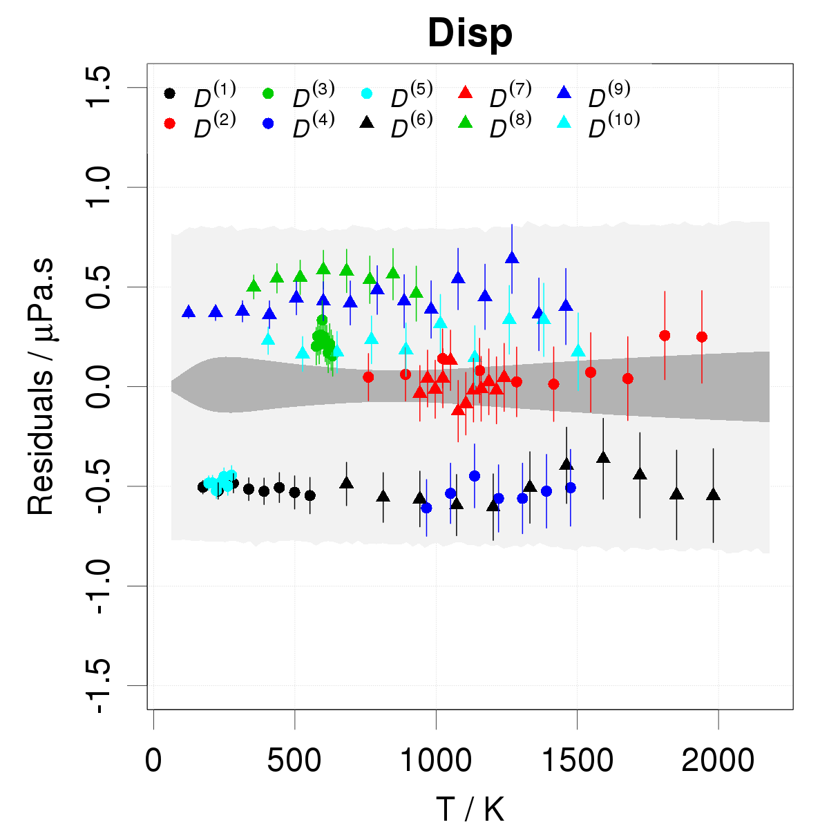
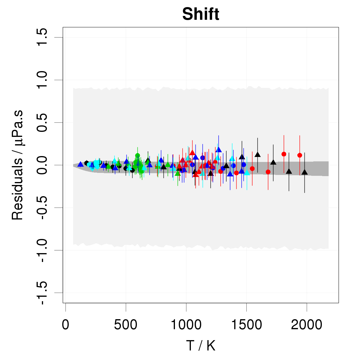
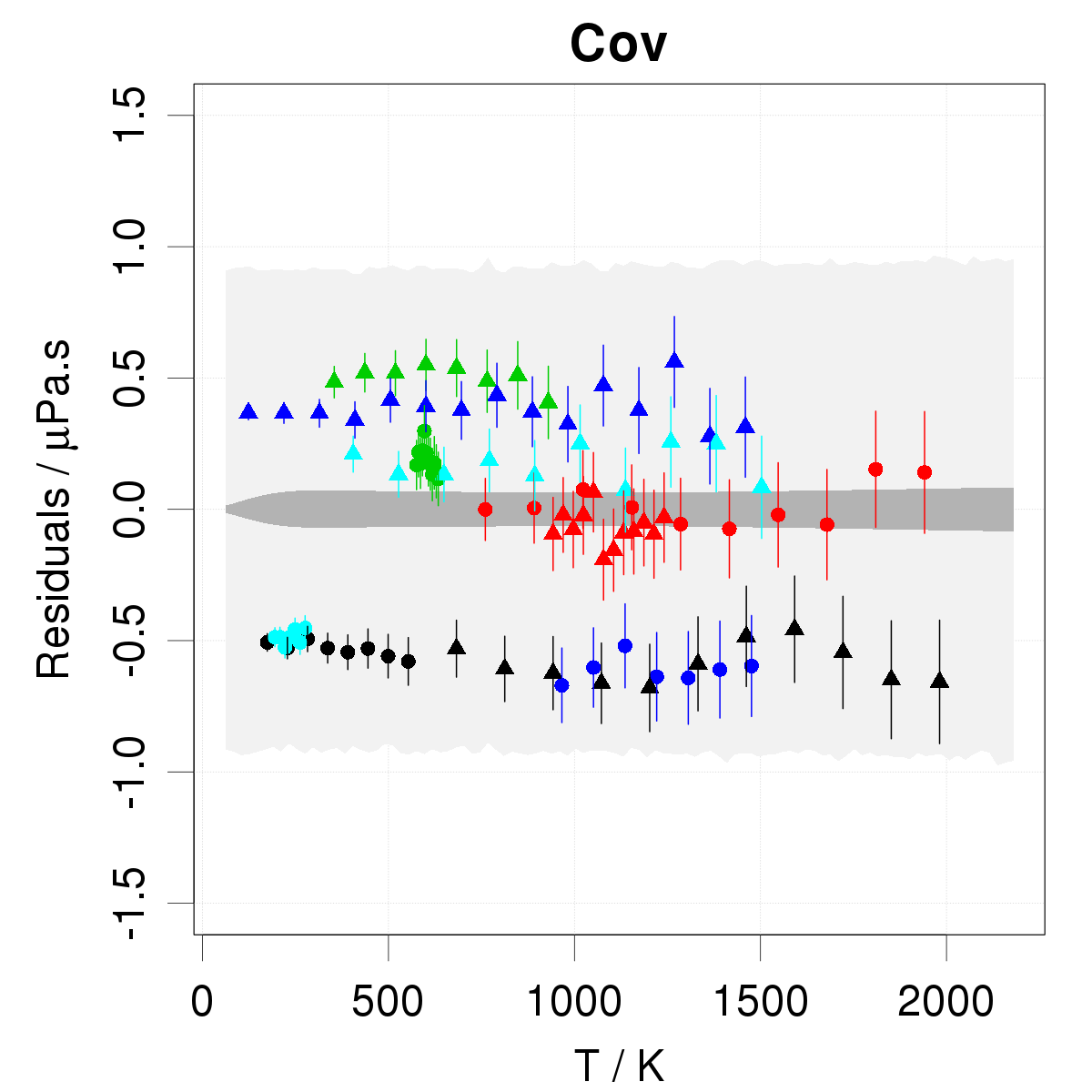
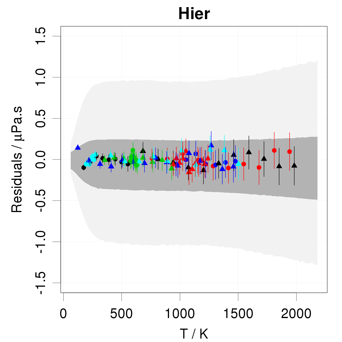
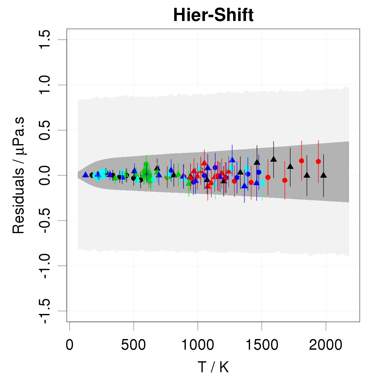
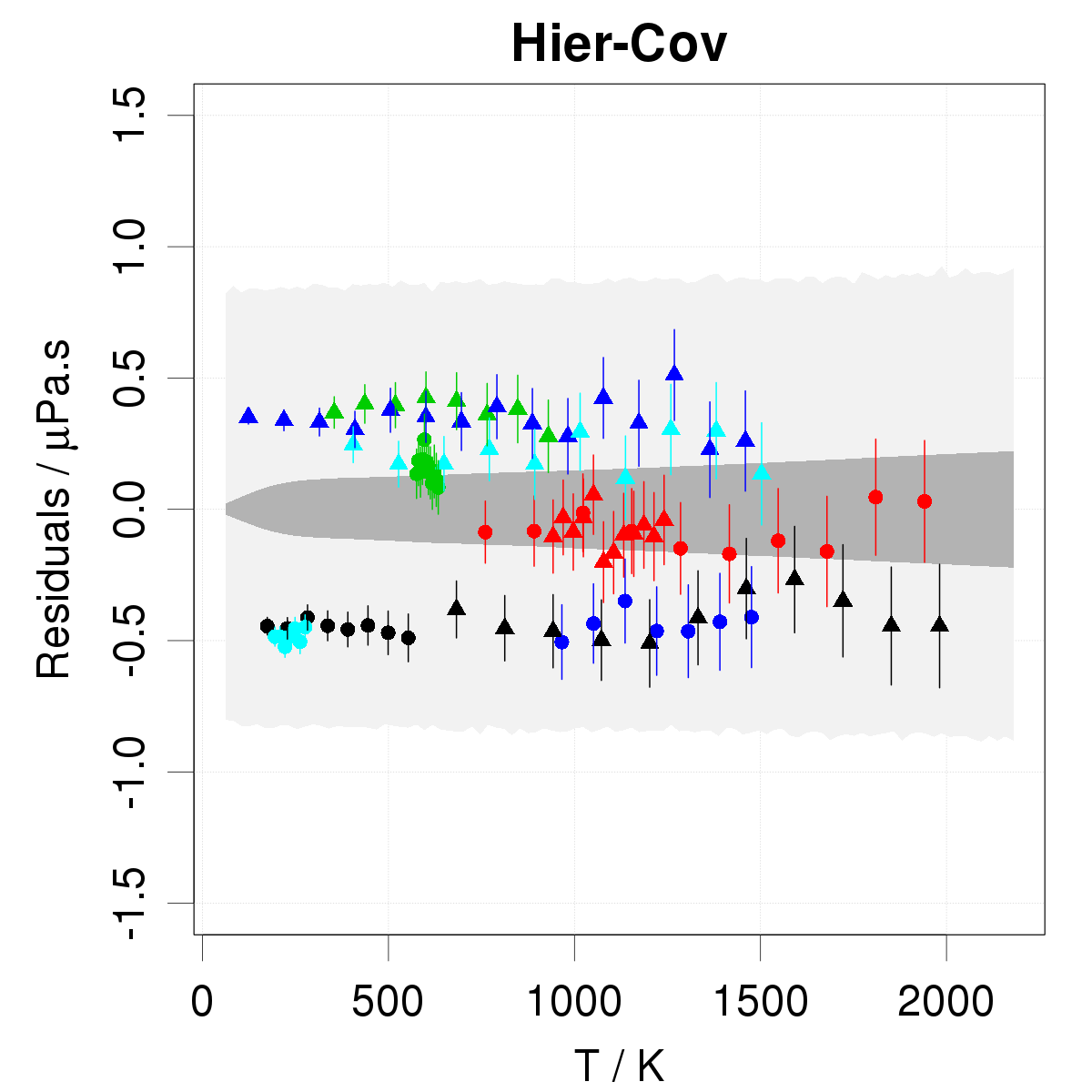
Figure 4: Calibration residuals and posterior prediction intervals for data SD-2. For each model, the results are centered on the maximum a posteriori results (MAP). The dark gray band represents the model prediction 95 % probability interval ($p_{M}$) and the light gray area the experiment prediction 95 % probability interval ($p_{e}$).

Model		$\epsilon_{LJ}$			$\sigma_{LJ}$			$\tau$		$MR$		$RMSD$		$R_{B}$		$u_{e|D}$
		(K)			(Å)			($\mu$Pa.s)		($\mu$Pa.s)		($\mu$Pa.s)				($\mu$Pa.s)
Ref		195			3.	6		0.42						1.00
Disp		195(2)			3.	602(4)		0.39(3)		0.00		0.39		1.00		0.40
Shift		195.	5(9)		3.	599(1)		0.4(1)		0.00		0.06		0.85		0.07
Cov		195.	5(9)		3.	599(1)		0.4(1)		-0.05		0.40		0.85		0.46
Hier		198(3)			3.	599(2)		-		-0.01		0.06		0.99		0.50
$u_{\epsilon},\,u_{\sigma}$		9(2)			0.	004(3)
$\rho$		-0.7(3)
Hier-Shift		197.	3(8)		3.	599(1)		0.4(1)		0.01		0.06		1.10		0.13
$u_{\epsilon},\,u_{\sigma}$		1(1)			0.	001(1)
$\rho$		0.0(6)
Hier-Cov		196(1)			3.	599(1)		0.4(1)		-0.04		0.39		0.98		0.43
$u_{\epsilon},\,u_{\sigma}$		0.	3(7)		0.	0008(8)
$\rho$		0.0(6)

Table 4: Summary of the main parameters and statistics for the methods tested on the SD-2 set. The first line (labeled Ref) provides reference value of the parameters and statistics.

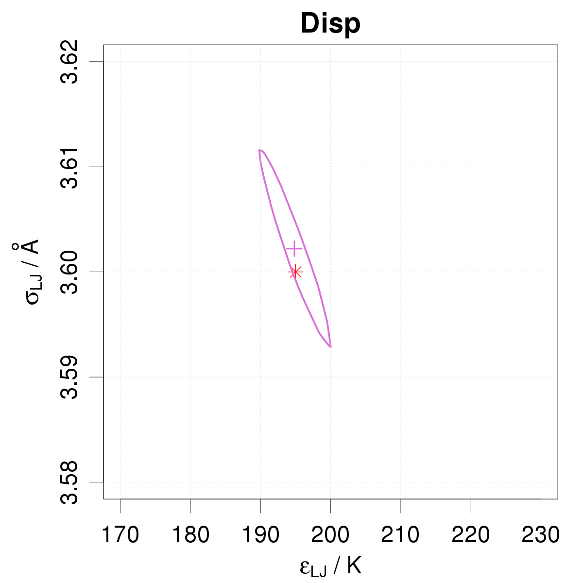
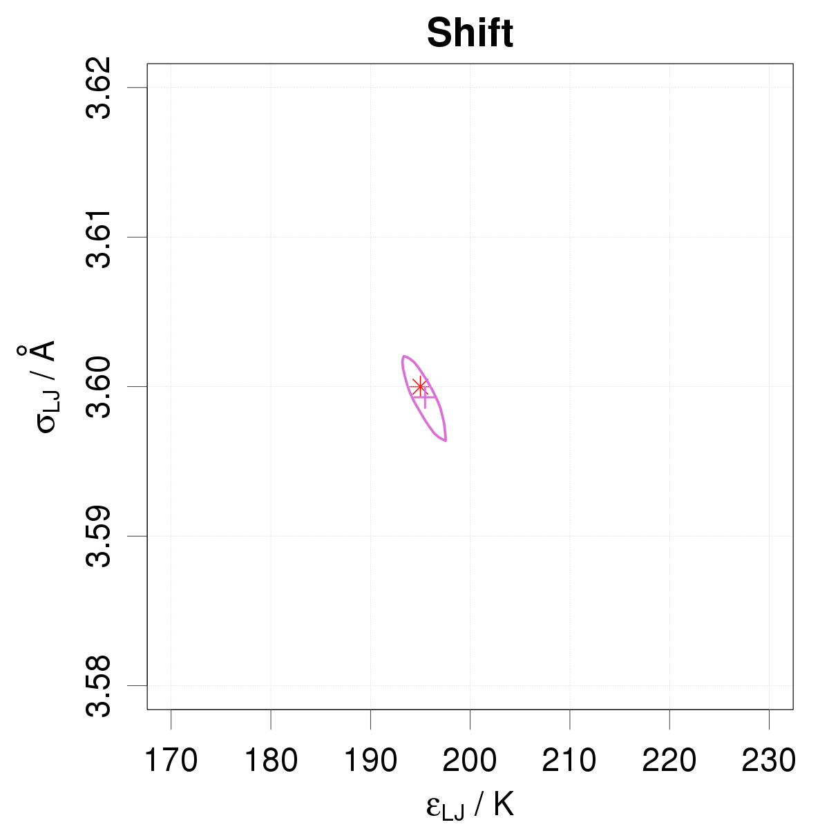
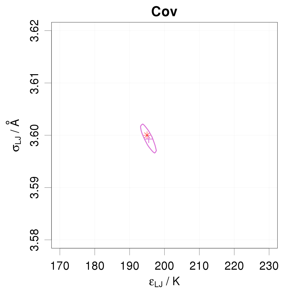
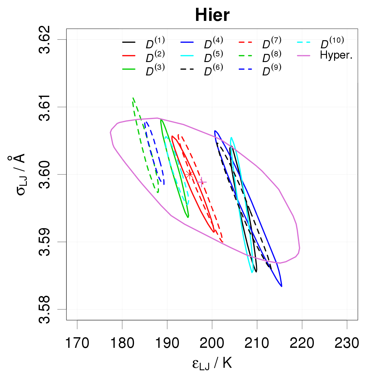
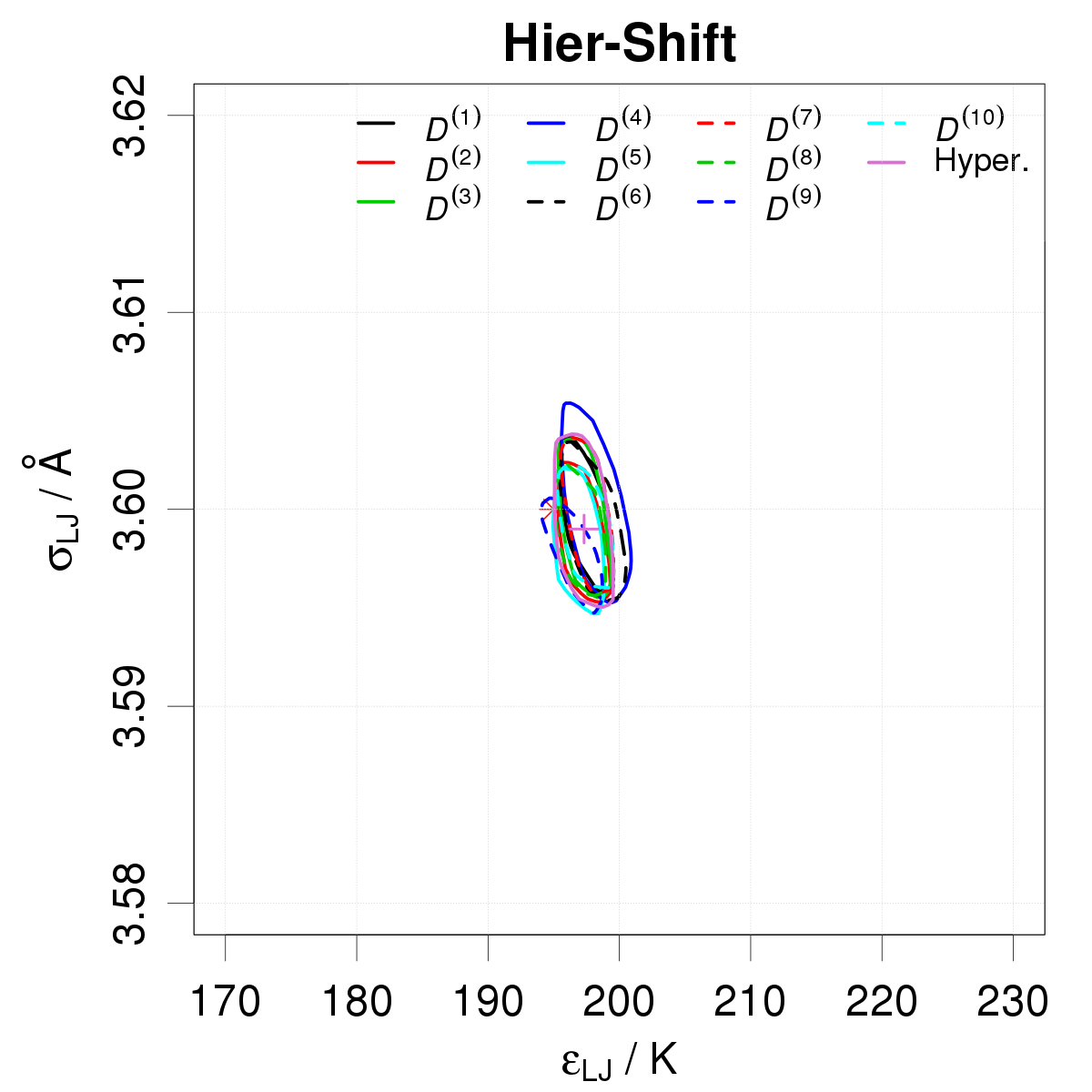
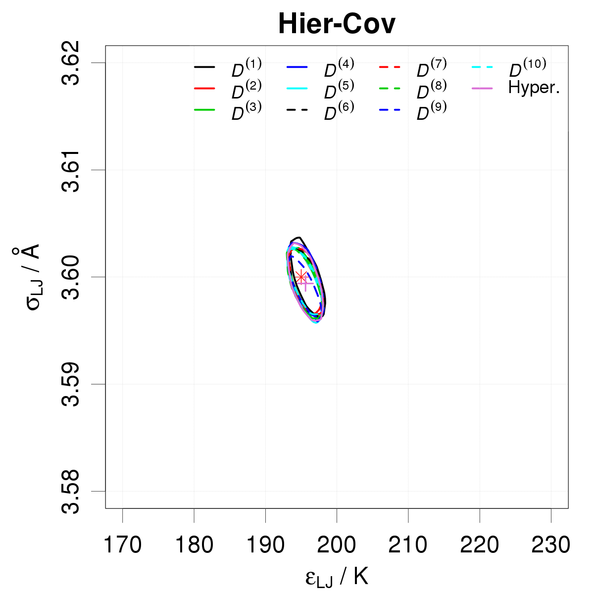
Figure 5: Posterior samples of LJ parameters calibrated on data SD-2: the elliptic contours represent 95 % probability intervals; the red cross depicts the reference value of the parameters.

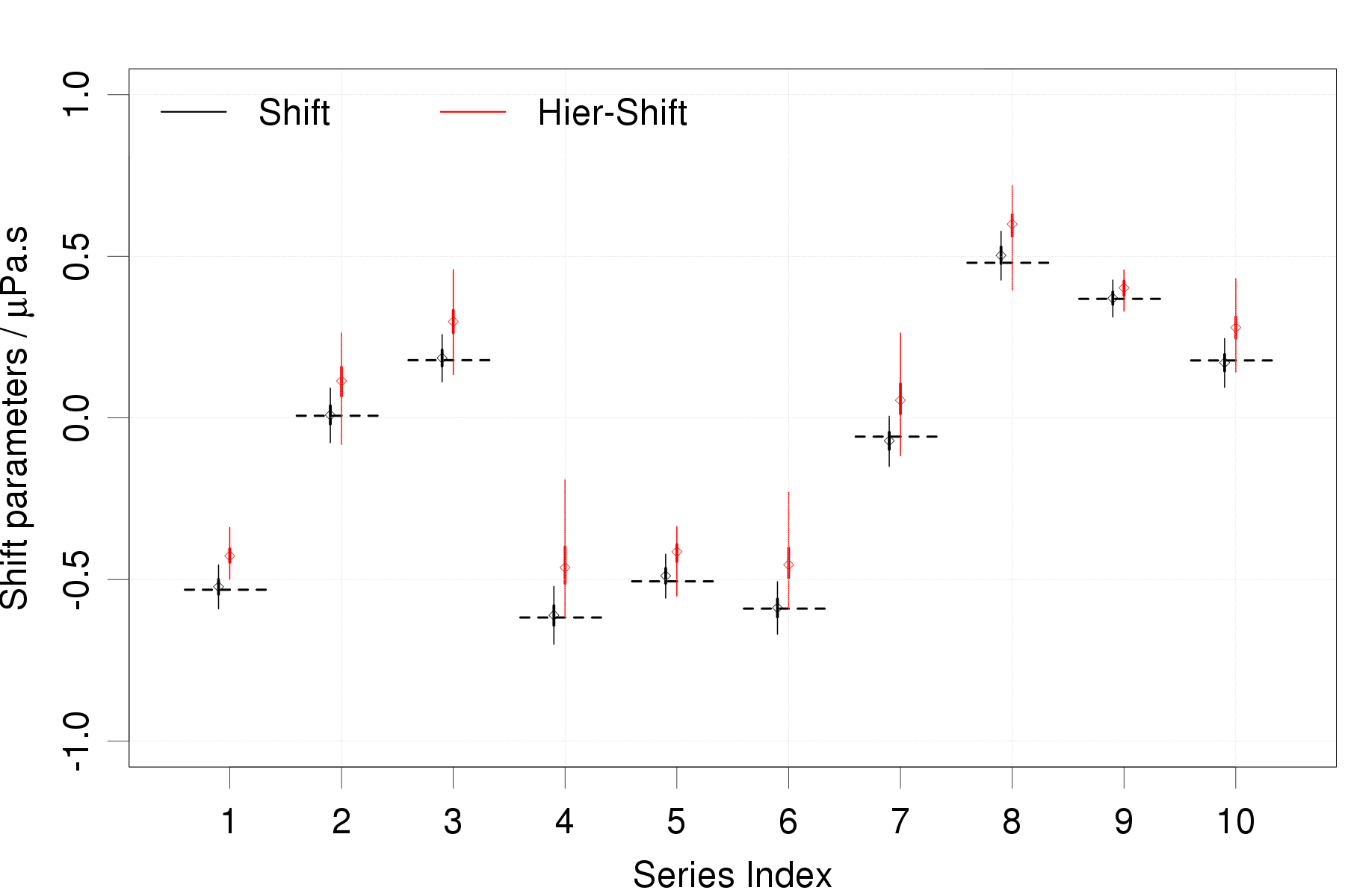
Figure 6: 95% confidence intervals for the shift parameters recovered by two methods from the SD-2 dataset. The horizontal bars represent the true values.

4.2.3 SD-3: model discrepancy & data inconsistency

We now use a dataset combining the two error sources of sets SD-1 and SD-2. This demands for a combination of the corresponding statistical models.

Simple models, such Disp are a priori unable to discriminate between the experimental and model systematic error sources. More promising methods can be obtained by combining the GP, ABC and Hier approaches of model discrepancy with Shift and Cov treatments of systematic experimental errors. The GP , Margin and ABC methods require a good estimation of model errors to be efficient. We have seen above (Section 4.2.2) that only the Shift method was able to provide residuals corrected for the systematic experimental errors. It is therefore the choice complement for the GP and ABC approaches. On the other hand, as shown in case SD-2, the Hier method can benefit from the Cov model, taking advantage of its smaller number of parameters. We consider therefore the following models: Disp for reference; Disp-Shift; GP-Shift; Margin-Shift; ABC-Shift; Hier-Shift; and Hier-Cov.

The models involving the determination of experimental shifts might present a parameter identification problem. If one does not constrain the shifts, the correction term $\delta M$ of the GP model attempts to compensate for them, and the model prediction is contaminated by the variance for systematic measurement errors. The problem occurs also for the ABC and Hier approaches, more strongly for the latter, as it uses individual LJ parameters sets for each data series. In order to avoid this problem, the sum-to zero constraint (Eq. 25) has been imposed in all shift-based methods.

The residuals of the Disp-Shift method (Table 5), with a $RMSD$ of $0.10$ $\mu$Pa.s, provide a scale for model inadequacy. Despite the additional constraint on the shift parameters, the GP-Shift method achieves a $RMSD$ value close to the random noise limit ($0.06$ $\mu$Pa.s). Comparing the residuals of the Disp and Hier-Cov methods, one sees how the Hier method attempts to compensate for the systematic experimental errors by adjusting the local LJ parameters.

All methods have adequate mean prediction uncertainty, except Hier-Shift and Hier-Cov for which it exceeds strongly the $RMSD$, as observed for the Hier method in case SD-1. This is visible in the large dispersion of the LJ parameters for these methods, notably $\sigma_{LJ}$ (Fig. (8)).

In terms of prediction bands, the Disp-Shift method provides adequate uncertainty bands for the model and experiment predictions (Fig. 7). The GP-Shift and Hier-Shift methods both correct well for model inadequacy, at least in large part, but provide very different MPUs. In fact, both the Hier-Shift and Hier-Cov methods produce unacceptably large prediction bands. In contrast, the model prediction band for ABC-Shift seems too narrow, notably at low temperature. The Margin-Shift method provides a structured prediction band with adequate covering of the residuals.

Distributions of shift parameters recovered by the five pertinent methods are shown in Fig. 9, and compared with the exact values. The sum-to-zero constraint introduces a slight bias in the recovered values, but they are well identified. As seen for case SD-2, only the Hier-Shift method provides large uncertainties on these shifts, due to their strong interaction with the local LJ-parameters of the Hier approach.

From this dataset with mixed experimental and model systematic errors, only the Disp-Shift, GP-Shift, Margin-Shift and ABC-Shift methods provide adequate prediction intervals. The Hier-based methods are strongly overestimating parameter uncertainty and prediction uncertainty.

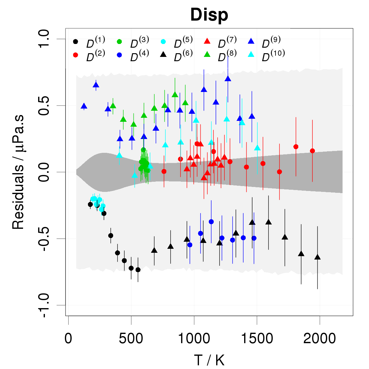
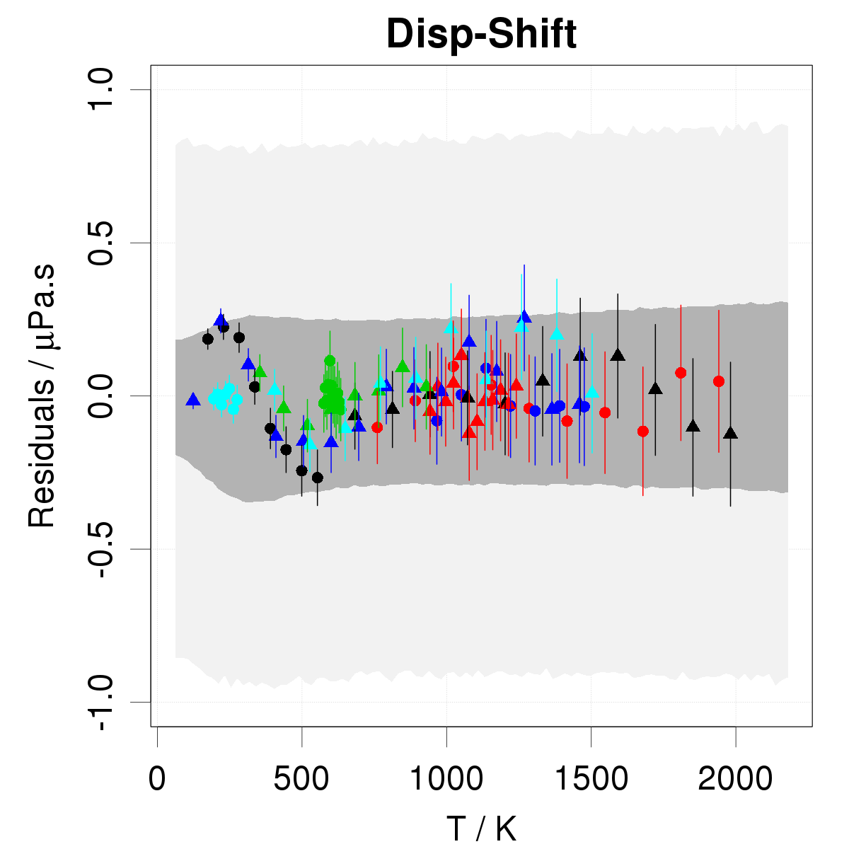
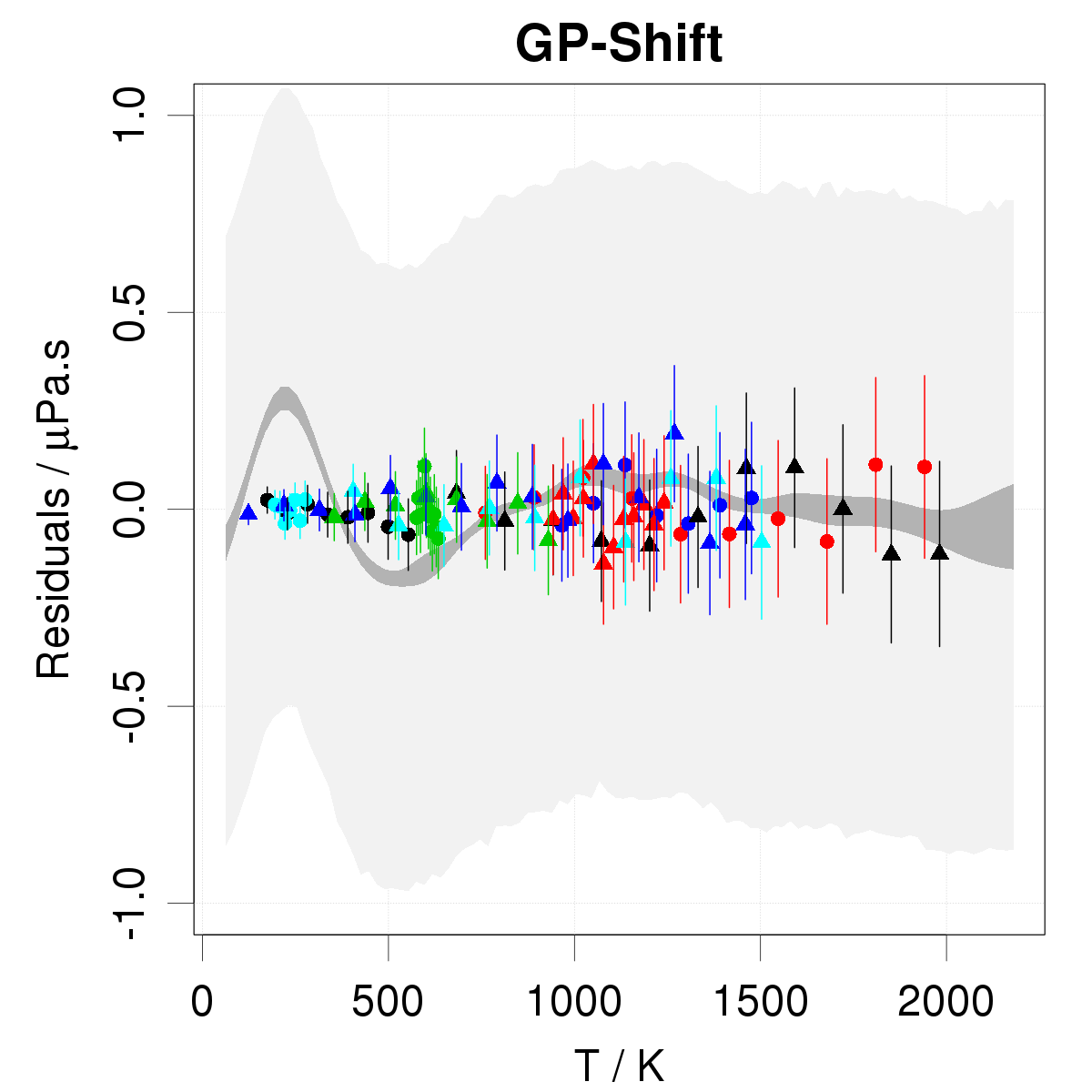
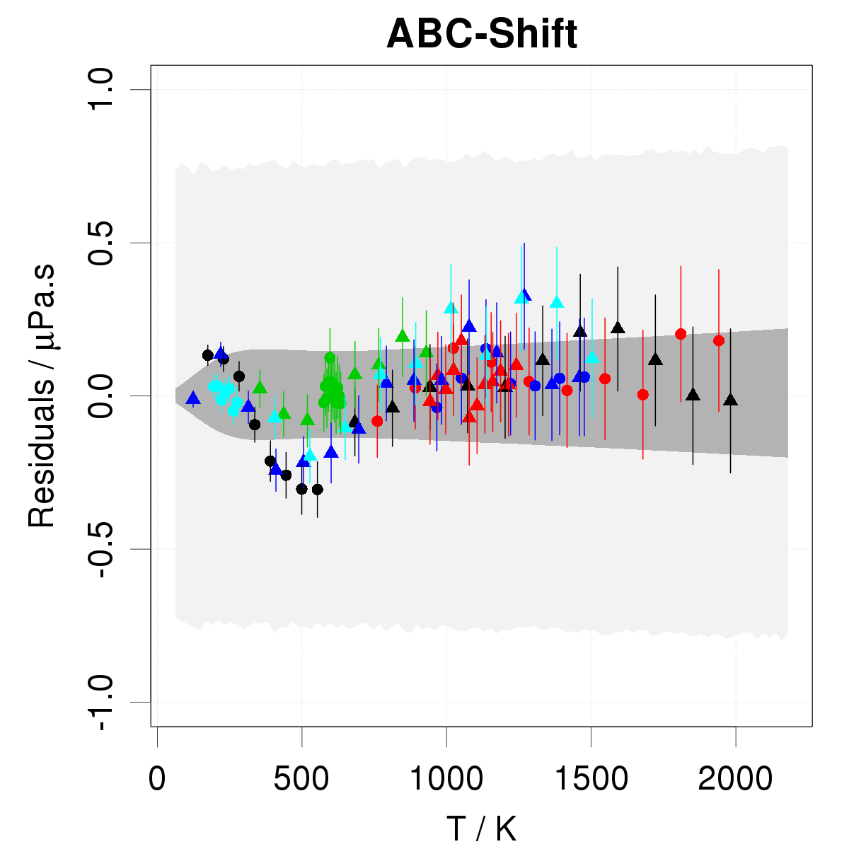
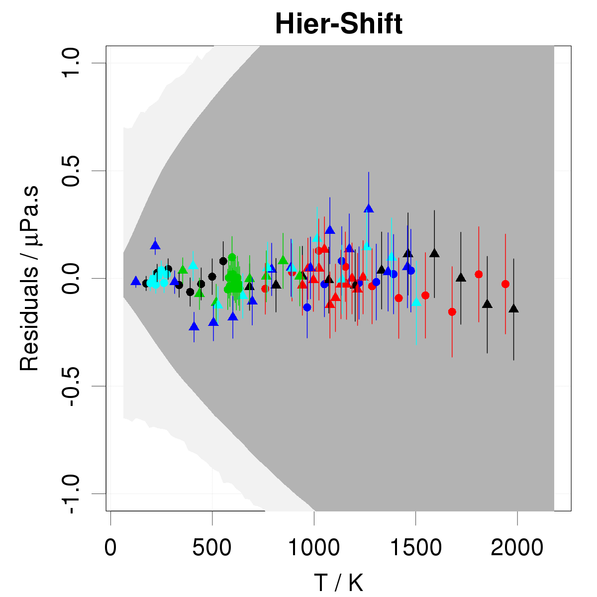
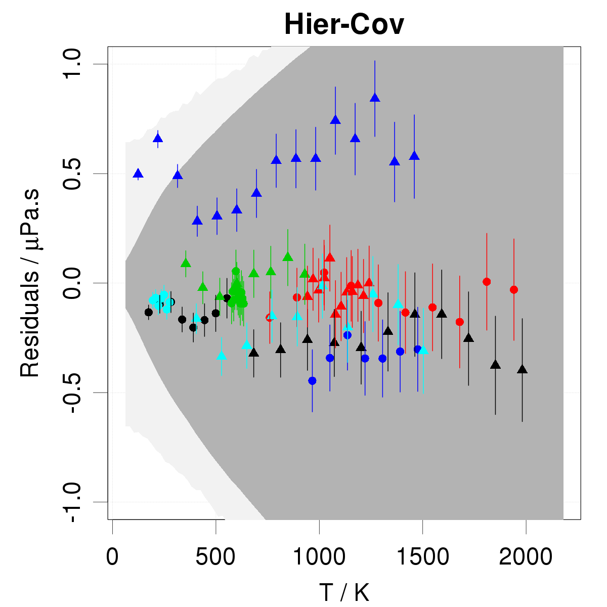
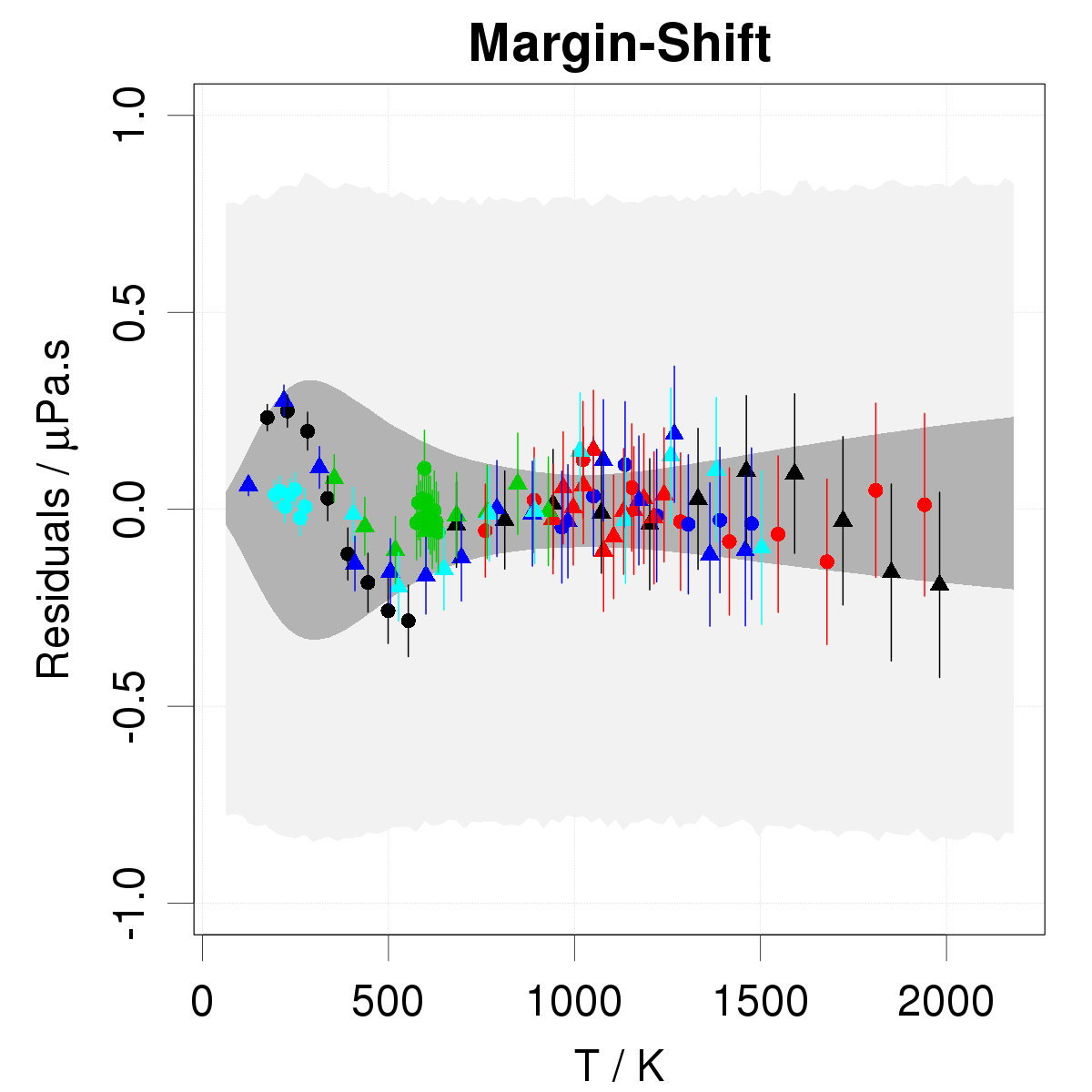
Figure 7: Calibration residuals and posterior prediction intervals for data SD-3. For each model, the results are centered on the maximum a posteriori results (MAP). The dark gray band represents the model prediction 95 % probability interval ($p_{M}$) and the light gray area the experiment prediction 95 % probability interval ($p_{e}$).

Model		$\epsilon_{LJ}$		$\sigma_{LJ}$		$\sigma$		$\tau$		$MR$		$RMSD$		$R_{B}$		$u_{e|D}$
		(K)		(Å)		($\mu$Pa.s)		($\mu$Pa.s)		($\mu$Pa.s)		($\mu$Pa.s)				($\mu$Pa.s)
Ref		195		3.6				0.42						1.00
Disp		255(3)		3.528(4)		0.37(3)		-		0.00		0.37		1.00		0.38
Disp-Shift		263(3)		3.523(2)		0.094(9)		0.4(1)		0.00		0.10		1.00		0.12
GP-Shift		260(3)		3.524(2)		-		0.40(6)		0.00		0.06		0.81		0.07
Margin-Shift		260(2)		3.522(2)		-		0.38(9)		-0.01		0.10		1.00		0.12
$u_{\epsilon},\,u_{\sigma}$		6(1)		0.007(2)
$\rho$		-0.99(1)
ABC-Shift		252.7(5)		3.5335(8)		-		0.36(9)		0.03		0.12		2.00		0.11
$u_{\epsilon},\,u_{\sigma}$		1.7(2)		0.0005(4)
$\rho$		-0.2(6)
Hier-Shift		253(2)		3.535(6)		-		0.32(9)		0.01		0.08		3.90		0.57
$u_{\epsilon},\,u_{\sigma}$		2(3)		0.016(5)
$\rho$		-0.3(5)
Hier-Cov		253(2)		3.535(6)		-		0.31(8)		0.07		0.31		3.50		0.66
$u_{\epsilon},\,u_{\sigma}$		2(3)		0.016(5)
$\rho$		-0.3(5)

Table 5: Summary of the main parameters and statistics for the methods tested on the SD-3 set. The first line (labeled Ref) provides reference value of the parameters and statistics.

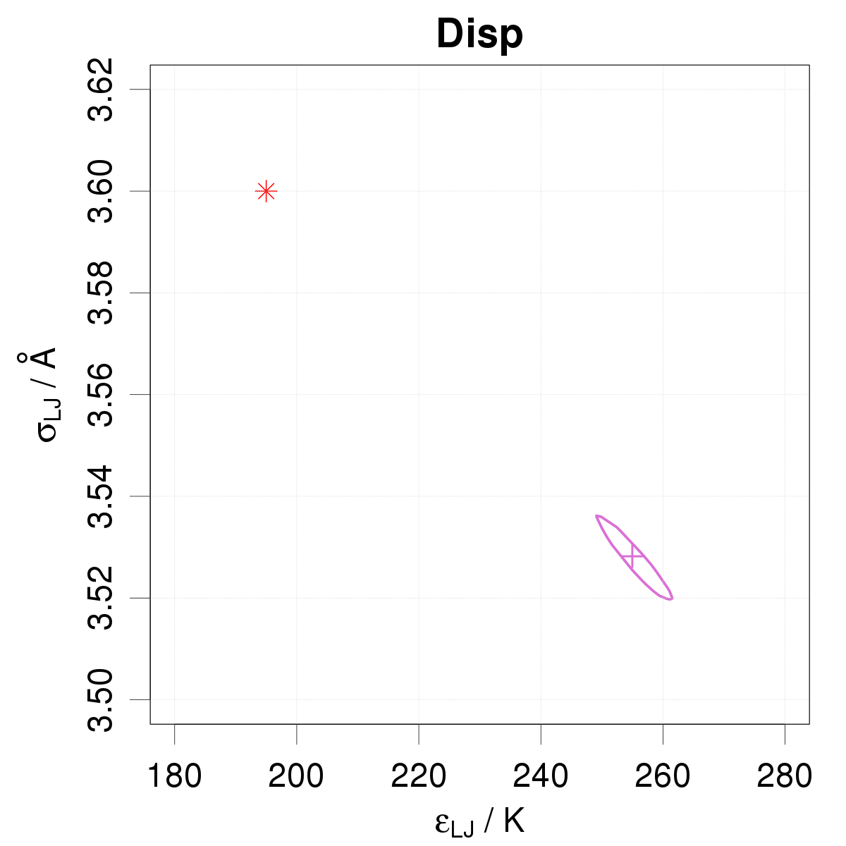
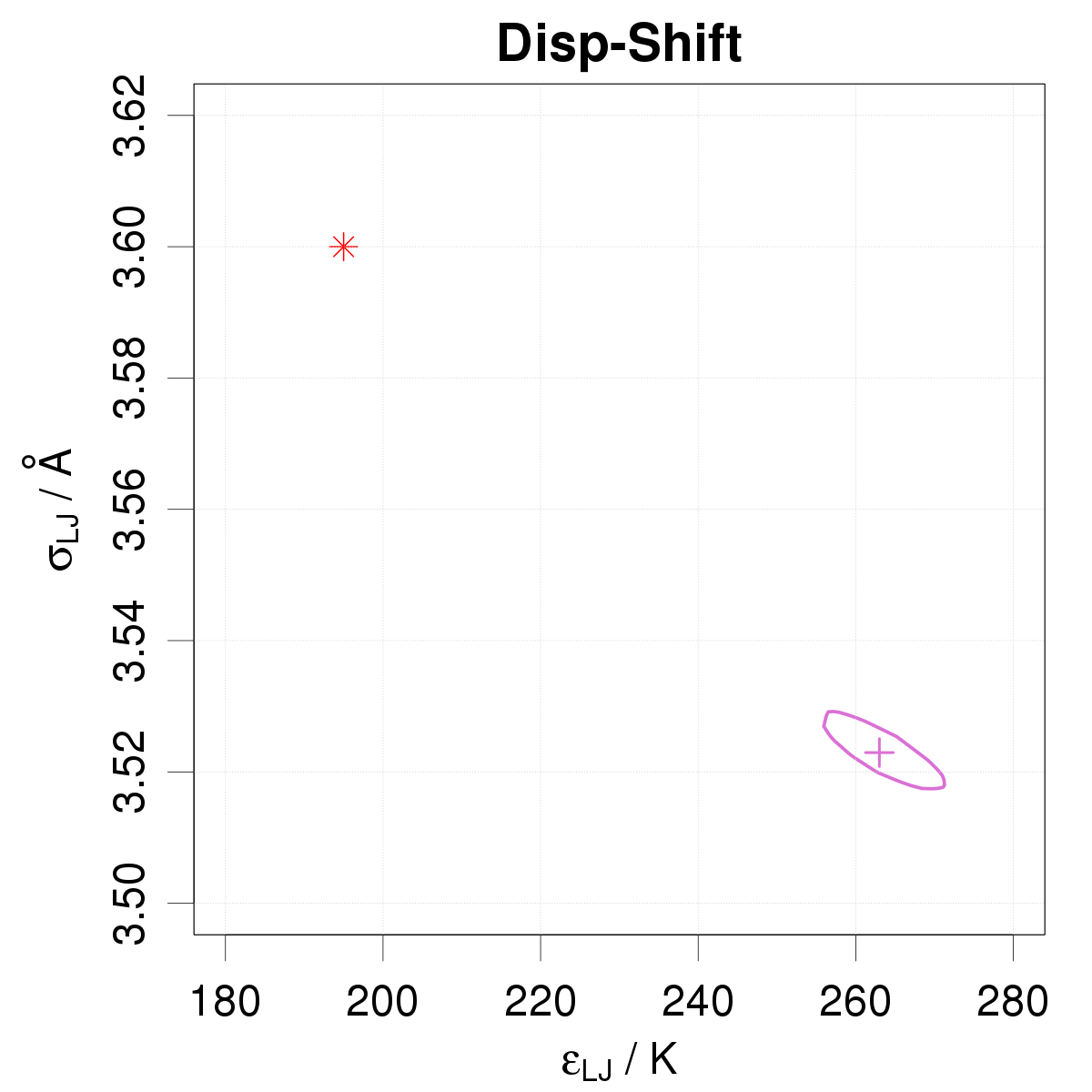
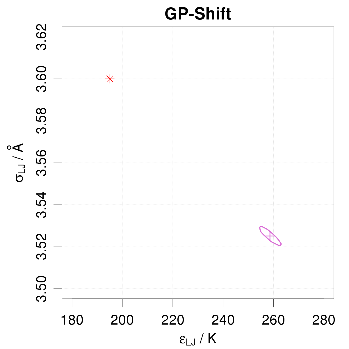
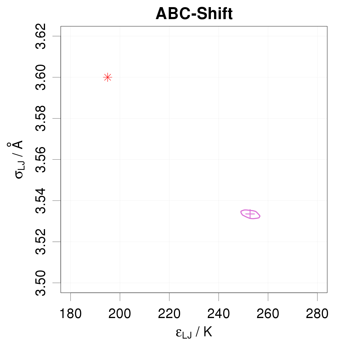
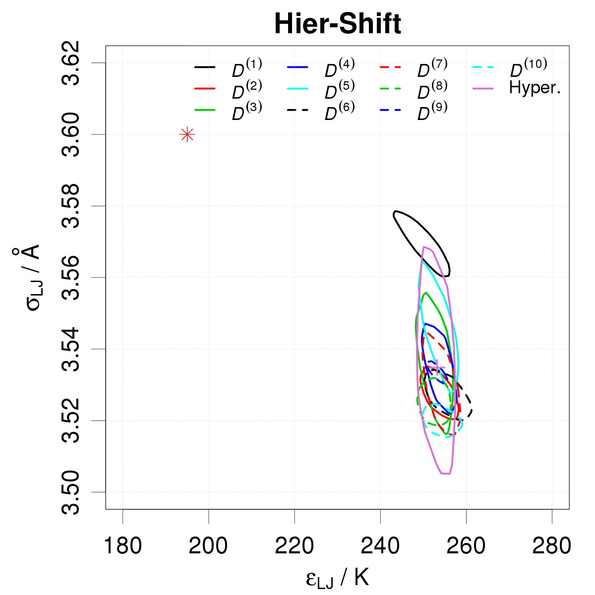
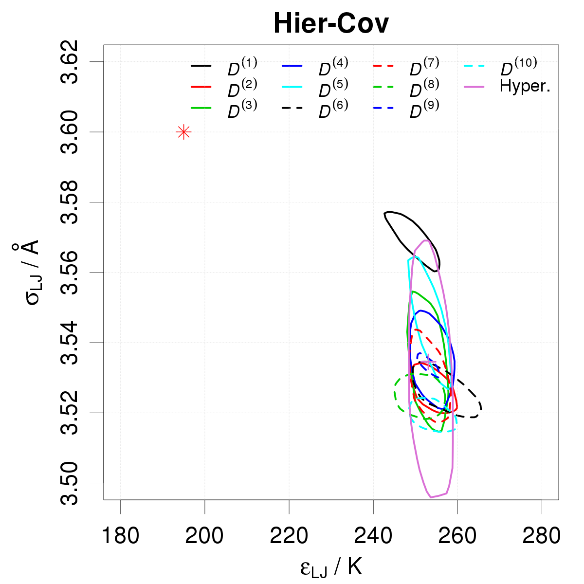
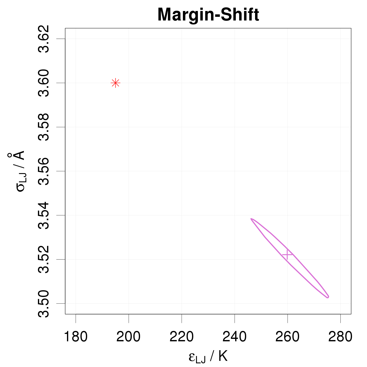
Figure 8: Posterior samples of LJ parameters calibrated on data SD-3: the elliptic contours represent 95 % probability intervals; the red cross depicts the reference value of the parameters.

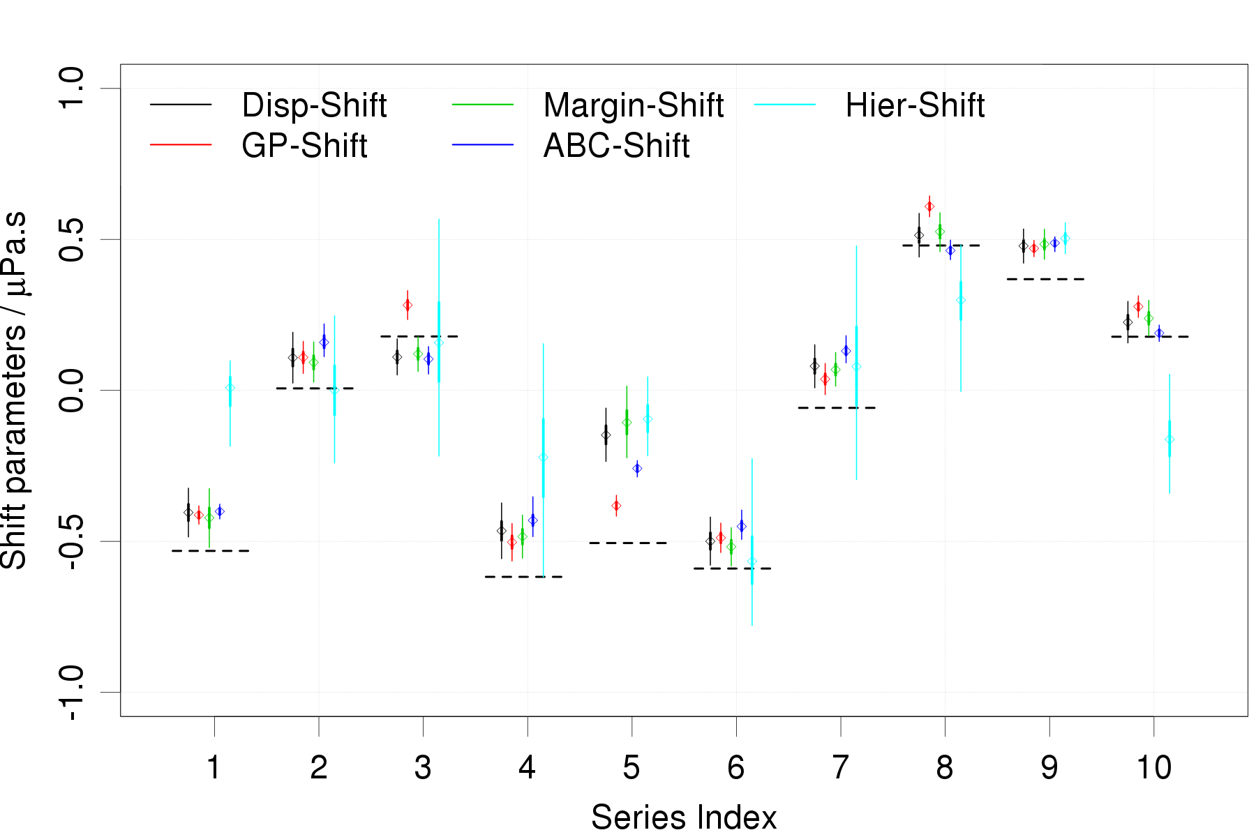
Figure 9: 95% confidence intervals for the shift parameters recovered by five methods from the SD-3 dataset. The horizontal bars represent the true values.

4.3 Krypton viscosity

We revisit now an example used by Wu et al. [9] to illustrate their hierarchical bayesian model, which aims to account for discrepancy between series in a compound set of data originating from several experimental setups and physical conditions. This example is a real-life realization of the synthetic SD-3 set and we test the same set of methods, except the Hier method defended by Wu et al. [9] ($\mathcal{M}_{H1}$model) and its variants Hier-Shift and Hier-Cov, which have been invalidated on the synthetic datasets.

The dataset used here includes 50 points from 5 series of viscosity measurements for Kr at temperatures covering a 120 – 2000 K range. These experiments have been evaluated and selected by Bich [78] in his review of the viscosity of monoatomic gases, where measurement uncertainties are also provided for all data. The dataset and references are provided in Appendix B.

The calibration/prediction results are shown in Figs. 10, 11, and Table 6.

Let us first consider the fit of the dataset by the Disp method, in order to appraise the structure of the residuals (Fig. 10). The standard deviation of the residuals is $0.44$ $\mu$Pa.s, and they display a strong serial correlation. The maximal deviation of the residuals is about $0.8$ $\mu$Pa.s, whereas the dispersion between data series in the $500$-$1000$ K range is about 5 times smaller. Series $D^{(3)}$ and $D^{(5)}$ are separated by more than $1$ $\mu$Pa.s between $1100$ and $1600$ K. The data are clearly inconsistent above $1000$ K. Model inadequacy is revealed by the marked tendencies of the residuals, within each series, and overall.

Looking at the $RMSD$, the best results are achieved, as expected, by the GP-Shift model. However, it is not able to resolve fully the residual inconsistency between series $D^{(1)}$, $D^{(3)}$ and $D^{(5)}$ after correction by shift factors, hence a slightly large Birge ratio ($1.3$). With a Birge ratio of $2.1$, the ABC-Shift method achieves a slightly poorer performance than the Disp-Shift and Margin-Shift methods, as observed in the SD-3 case. It provides a rather too narrow model prediction band, notably for the low-T series, $D^{(4)}$.

The posterior pdfs for the parameters of ABC-Shift and Margin-Shift are bimodal (Appendix C). As seen for SD-1, the modes correspond to extreme values of the hyperparameters describing the covariance matrix of the LJ parameters. In the present case both methods explore the modes corresponding to (1) $\rho\simeq-1$ and (2) very small values of $u_{\sigma}$. In case SD-1, the posterior samples for these methods were located each on one of these modes. The increase in parameters uncertainty due to the smaller reference data set might be responsible for the multimodality. In fact, a trimodality, involving the mode with very small values of $u_{\epsilon}$, was formerly observed by Pernot [49] for the calibration of Ar viscosity data with 41 points.

The shifts inferred by the relevant methods are shown in Fig. 12. They are in global agreement, with a larger inter-method dispersion for series $D^{(4)}$ and $D^{(5)}$.

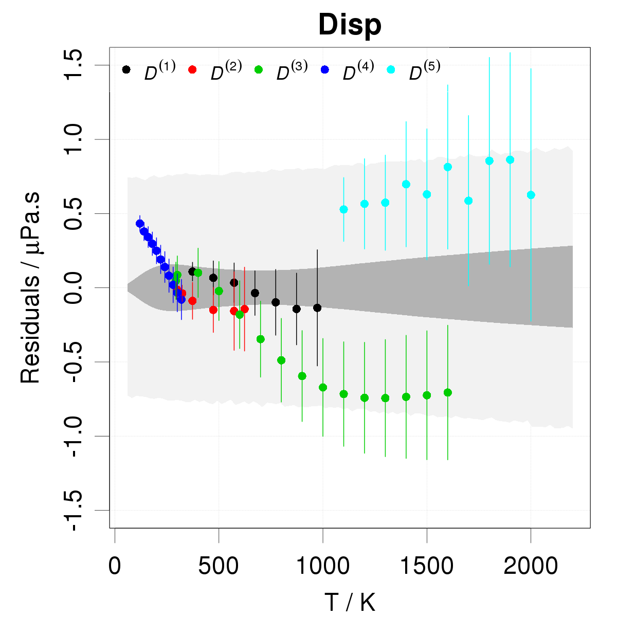
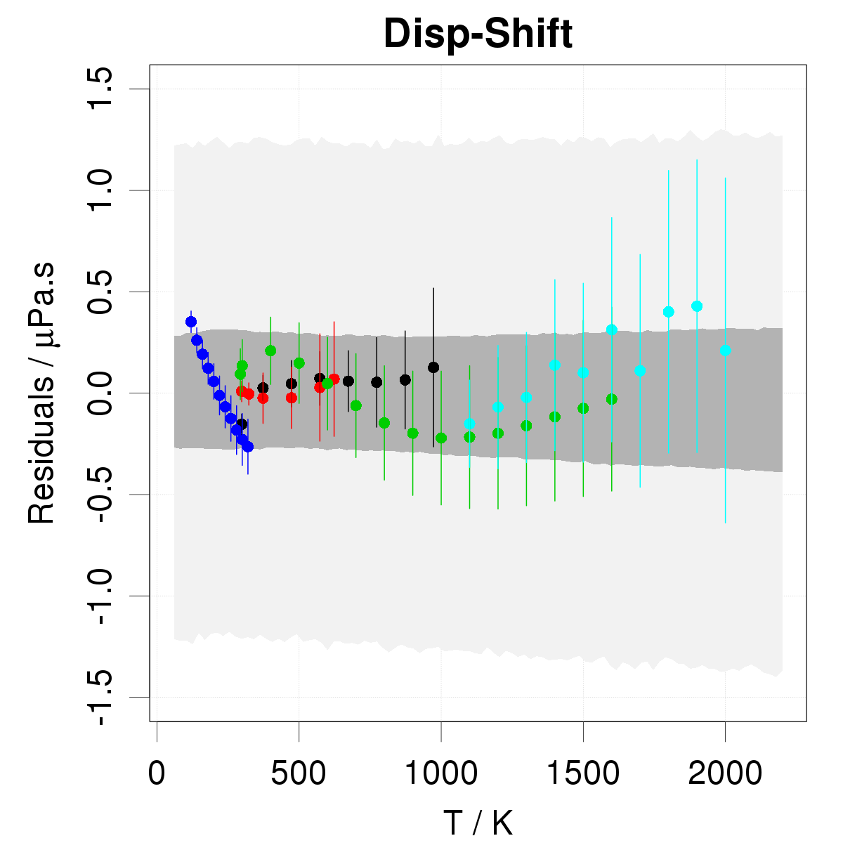
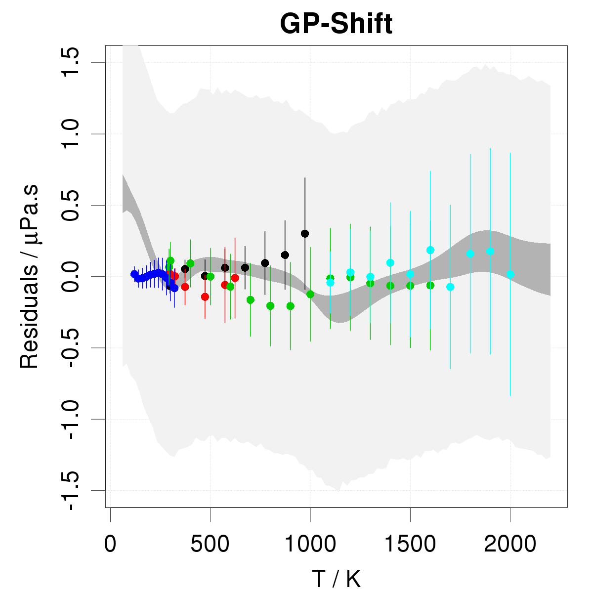
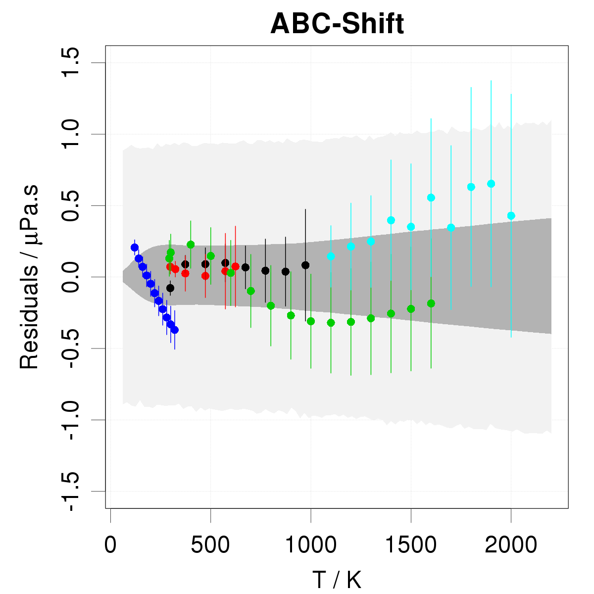
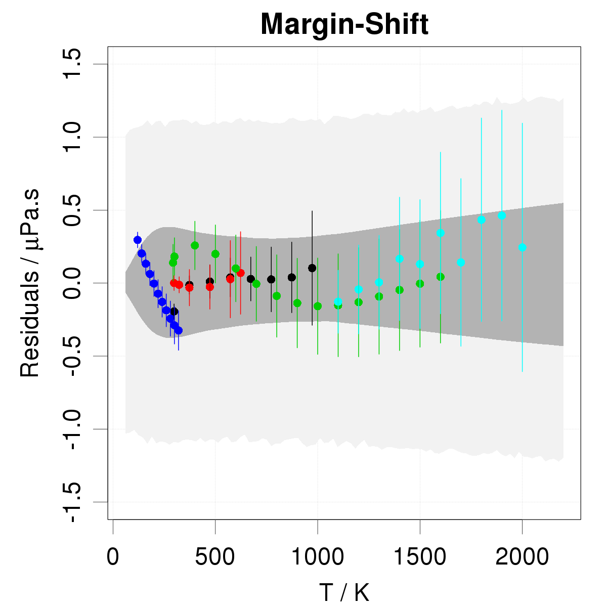
Figure 10: Calibration residuals and posterior prediction intervals for the Krypton set. For legibility, one has subtracted the best fit to all curves. The dark gray area represents model prediction 95 % probability ($p_{M}$) and the light gray area experiment prediction 95 % probability ($p_{e}$).

Model		$\epsilon_{LJ}$		$\sigma_{LJ}$		$\sigma$		$\tau$		$MR$		$RMSD$		$R_{B}$		$u_{e|D}$
		(K)		(Å)		($\mu$Pa.s)		($\mu$Pa.s)		($\mu$Pa.s)		($\mu$Pa.s)				($\mu$Pa.s)
Disp		204(3)		3.535(5)		0.37(5)		-		0.03		0.44		1.20		0.41
Disp-Shift		192(2)		3.559(4)		0.14(2)		0.6(2)		0.02		0.16		0.96		0.22
GP-Shift		192(2)		3.559(4)		-		0.6(1)		0.00		0.10		1.30		0.16
Margin-Shift		193(2)		3.557(5)		-		0.5(2)		0.03		0.17		0.93		0.24
$u_{\epsilon},\,u_{\sigma}$		5(1)		0.007(4)
$\rho$		-0.8(4)
ABC-Shift		196.5(8)		3.550(2)		-		0.3(1)		0.02		0.24		2.10		0.20
$u_{\epsilon},\,u_{\sigma}$		3(1)		0.004(4)
$\rho$		-0.5(6)

Table 6: Summary of the main parameters for the methods tested on the Krypton set.

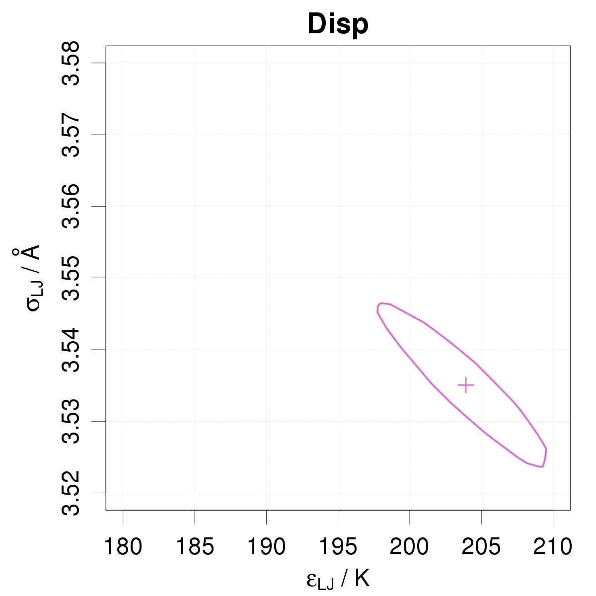
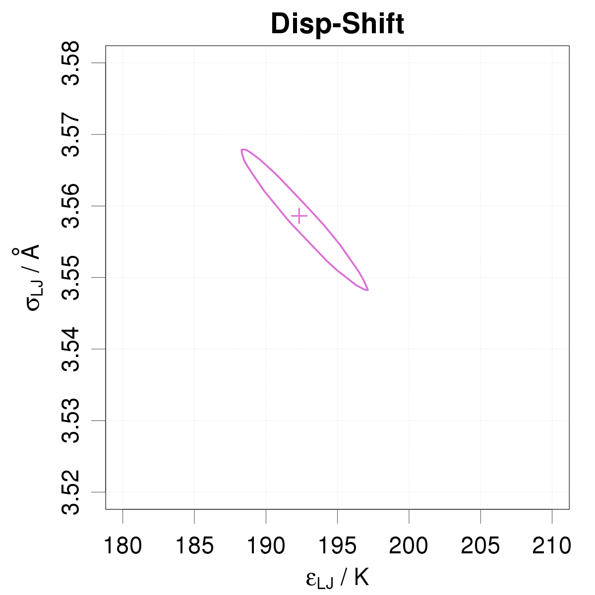
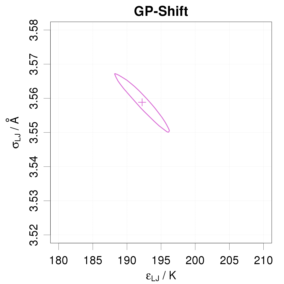
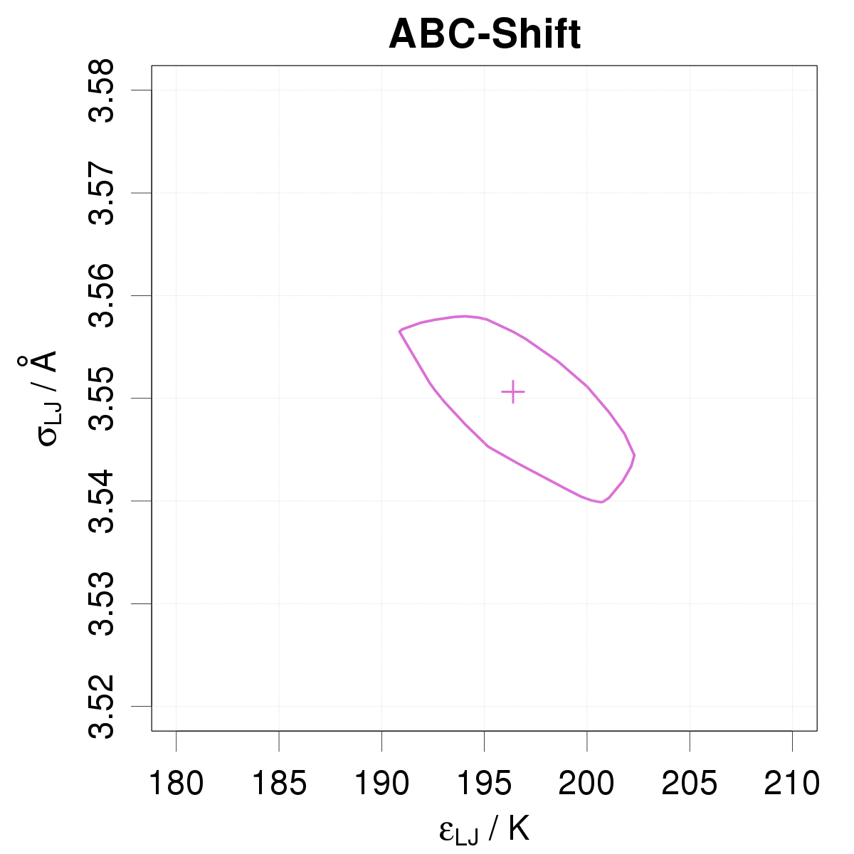
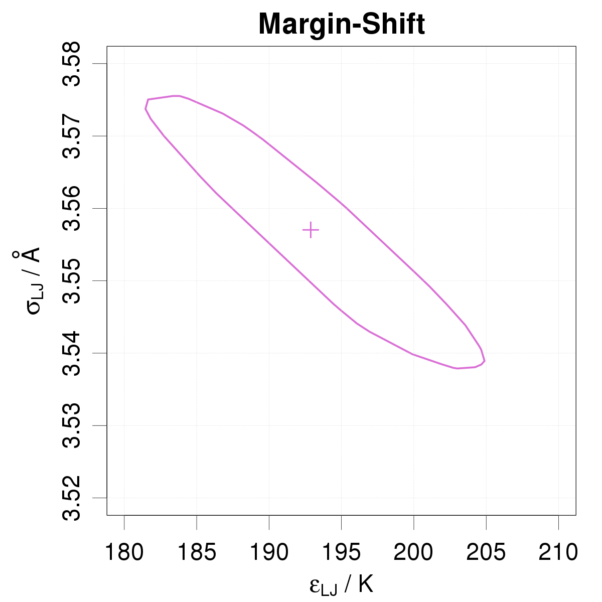
Figure 11: Posterior samples of LJ parameters calibrated on the Kr dataset: the elliptic contours represent 95 % probability intervals.

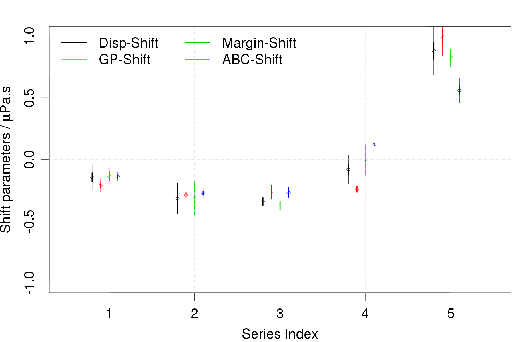
Figure 12: 95% confidence intervals for the shift parameters recovered by four methods from the Kr dataset.

5 Discussion

A first observation resulting from the analysis of cases SD-1 and SD-3 is that LJ parameters are very sensitive to model inadequacy, and that none of the tested methods includes the true value of the parameters in its posterior pdf/sample, even those correcting and/or accounting for model discrepancy. Model improvement is the only way to infer unbiased values of physical parameters. On the other hand, effective values of the parameters can still be used to provide useful predictions.

5.1 Error sources discrimination

Among the methods proposed in the literature to deal with calibration/prediction of physico-chemical models, not all are able to deal with the combination of inconsistent data and model errors. The numerical experiments in the previous section have shown that it is essential to treat both error sources by distinct/complementary statistical models. This is well achieved by combination methods, such as Disp-Shift, GP-Shift, Margin-Shift and ABC-Shift.

Wu et al. [9] have proposed a hierarchical model on the LJ parameters to analyze “cross-experiment uncertainty” because it provides a higher prediction uncertainty than the standard model. In our simulations, the idea of absorbing data inconsistency in parameters uncertainty (model Hier) has been shown to fail systematically by leading to (largely) overestimated prediction uncertainties. Even when combining this approach with an explicit treatment of data inconsistency (models Hier-Shift or Hier-Cov), the interactions between LJ parameters and shift parameters lead to exaggerated prediction uncertainties. Note that this is not a global rejection of hierarchical modeling, which is perfectly sound and useful to infer, for instance, the shifts of inconsistent datasets (model Shift).

5.2 Posterior pdf multimodality in ABC & Margin

In PUI methods describing the ensemble of the LJ parameters by a multivariate normal distribution $p(\boldsymbol{\vartheta}_{M}|\boldsymbol{\mu}_{\vartheta_{M}},\boldsymbol{V}_{\vartheta_{M}})$, one observes typically a concentration of the hyperparameters on one or several of the modes corresponding to extreme values of the covariance matrix parameters, $u_{\sigma}$, $u_{\epsilon}$ and $\rho$ in the present 2D case. The Margin method tends to favor an extreme negative correlation coefficient ($\rho\simeq-1$), which is not the case for the ABC method, leading to different parameter samples and prediction bands. Besides the fact that it makes these methods difficult to calibrate if one has not a good prior for the hyperparameters, the multimodality might be problematic in the sense that it makes the prediction bands very sensitive to the details of the calibration dataset. Except maybe for very large calibration datasets, adding more calibration data might shift the posterior pdf of the parameters onto one or the other mode in an unpredictable way. As shown by Pernot [49], the prediction bands corresponding to the three modes have different geometries, and mode-shifting or the redistribution of probability among modes might result in radical changes in the shape of prediction bands.

5.3 VarInf-type methods

The simple PUI methods based on data variance scaling (VarInf-type methods) have been shown to provide poorly reliable prediction bands. The scaling method based on the temperature analogy (Eq. 39) has been found in case SD-1 to provide exaggerated prediction uncertainty. A better mean prediction uncertainty was obtained with a prediction variance based criterion (Eq. 40). This approach cannot be recommended on a general basis, and should be carefully validated before being put into use.

5.4 Calibration transferability

A difficulty in calibration is the transferability of parameter uncertainty. In presence of model inadequacy, parameter uncertainty represents often a small contribution to MPU. In fact, unless there is an identification problem, parameter uncertainty resulting from a model calibration is expected to diminish when one increases the size of the calibration dataset, which is not the case for model inadequacy. The main issue is therefore the transferability of model inadequacy [47, 48]. Additive corrections to the model are not transferable to other observables than the ones for which the correction is designed. Methods such as Disp and GP, are therefore not useful outside of their calibration framework. As extensively discussed by Sargsyan et al. [46] an additional problem with these methods is the difficulty to constrain their predictions by physical rules or boundary limits. This might be notably problematic in sequential multiscale simulations if the predictions at one level violate physical constraints required at an upper level.

If transferability or such constraints are not an issue, we have shown that methods such as Disp and Disp-Shift are very interesting options, notably because they provide correct model inadequacy coverage and are easy to communicate and apply for further predictions [14].

The main approach that has been proposed in the literature to resolve the transferability problem is to embed model inadequacy in parameter uncertainty. Several methods to do this have been tested above: VarInf, Margin, ABC and Hier (Section 3.3.2). We have shown that they all suffer a priori from the problem of inadequate prediction bands, but our simulations have shown that the ABC and Margin method perform better than the other ones. Provided the reserves on this type of method expressed above, and considering that the Margin method has no or little room for improvement, the ABC method offers probably the most promising framework. One could for instance envision additional constraints on the prediction band shape in the ABC pseudo-likelihood function $p_{reg}$ (Eq. 48) for a better prediction reliability and stability.

6 Conclusion

We have reviewed and tested a series of standard and advanced statistical models used in the computational chemistry literature to calibrate physical models on experimental data. All models have been coded and run in the same bayesian framework in the stan language. Their prediction performances have been evaluated on synthetic and experimental data.

Focusing on the realistic scenario where measurement uncertainty, experimental (residual) systematic errors and model inadequacy contribute significantly to the error budget, we have shown that reliable calibration/prediction methods depend on the capture and disambiguation of all the error sources in the statistical analysis model. For instance, in order to do meaningful predictions, variables of the statistical model have to be unambiguously attributed to one of the error sources.

In this scenario, the best performing methods are the GP-Shift, Margin-Shift and ABC-Shift methods, both with advantages and drawbacks. The GP-Shift method provides a good interpolator, but it is not usable for extrapolation out of the calibration range nor to other observables. The Margin-Shift and ABC-Shift methods do not present the drawbacks of the GP approach, but their prediction bands are controlled by the model derivatives and do not necessarily conform with the observed error distribution. Moreover, we have shown that they are possibly unstable with regard to the calibration dataset.

The Hier(archical) methods proposed recently by Wu et al. [9] have been shown to systematically overestimate prediction uncertainty. On the one hand, the use of LJ parameters uncertainty to describe experimental systematic errors conflicts with our definition of unambiguous attribution of error sources. On the other hand, adaptation of LJ parameters to the calibration scale of temperature results in a parameter space too large to permit meaningful predictions. We cannot recommend these methods in our study cases.

There is at the moment no perfect and universal solution to the prediction problem of inadequate physical models [32]. If model inadequacy is the dominant source of uncertainty, and if the residuals are not structured, description of model inadequacy by a single stochastic variable is a robust and efficient alternative (Disp method) [14]. We have also shown that adapting the ABC method as proposed by Sargsyan et al. [46] to deal with random and systematic experimental errors offers a promising framework for reliable predictions and calibration transferability.

Supporting Information

The R scripts and stan codes necessary to reproduce the tables and figures of the article are available on github: https://github.com/ppernot/CalPred.

Appendix A Systematic errors, correlation and weighting

Let us consider two results of repeated measurements, $y_{1}$ and $y_{2}$, with a common, unknown, measurement bias (systematic error). The joint posterior pdf of the true value $\mu$ and the bias $s$ is

$$p(\mu,s|y_{1},y_{2},u,\tau) \propto u^{-1}\exp\left(-\frac{1}{2u^{2}}\left((y_{1}-\mu-s)^{2}+(y_{2}-\mu-s)^{2}\right)\right)$$ (56)

$$\times\tau^{-1}\exp\left(-\frac{1}{2}\frac{s^{2}}{\tau^{2}}\right)$$

where $u$ is the measurement uncertainty due to random effects, and $s$ is a priori normally distributed with mean $0$ and standard deviation $\tau$.

Integration on $s$ provides the marginal posterior for $\mu$

$$p(\mu|y_{1},y_{2},u,\tau) \propto \int p(\mu,s|y_{1},y_{2},u,\tau)\,ds$$ (57)

$$\propto \frac{1}{\sqrt{(u^{2}+\tau^{2})(1-\rho^{2})}}$$ (59)

$$\times\exp\left(-\frac{(y_{1}-\mu)^{2}-2\rho(y_{1}-\mu)(y_{2}-\mu)+(y_{2}-\mu)^{2}}{2(u^{2}+\tau^{2})(1-\rho^{2})}\right)$$

$$\propto (\det\mathbf{V})^{-1/2}\exp\left(-\frac{1}{2}\boldsymbol{R}^{T}\boldsymbol{V}^{-1}\boldsymbol{R}\right)$$ (60)

where

$$\boldsymbol{R}=\left(\begin{array}[]{c}y_{1}-\mu\\ y_{2}-\mu\end{array}\right),$$ (61)

$$\boldsymbol{V}^{-1}=\frac{1}{(u^{2}+\tau^{2})(1-\rho^{2})}\left(\begin{array}[]{cc}1&-\rho\\ -\rho&1\end{array}\right),$$ (62)

with correlation coefficient

$$\rho=\tau^{2}/(u^{2}+\tau^{2}).$$ (63)

The corresponding covariance matrix is thus

$$\boldsymbol{V}=(u^{2}+\tau^{2})\left(\begin{array}[]{cc}1&\rho\\ \rho&1\end{array}\right)$$ (64)

More generally, for $N$ data points, one can design a covariance matrix

$$\boldsymbol{V}=(u^{2}+\tau^{2})\left(\begin{array}[]{cccc}1&\rho&\cdots&\rho\\ \rho&1&\ddots&\vdots\\ \vdots&\ddots&\ddots&\rho\\ \rho&\cdots&\rho&1\end{array}\right),$$ (65)

from which the estimate for $\mu$ will be

$$\mathrm{E}[\mu]=\overline{y}$$ (66)

$$\mathrm{Var}[\mu]=\frac{1+(N-1)\rho}{N}\,(u^{2}+\tau^{2})$$ (67)

• for $\rho=0$, one recovers the limit of independent measurements and

  $$Var[\mu]=u^{2}/N,$$ (68)

• in the limit of very strong serial correlation ($\rho\simeq 1)$, i.e. in cases where the random measurement errors are negligible before the systematic error, one gets the maximal variance for $\mu$

  $$Var[\mu]=(u^{2}+\tau^{2})\simeq\tau^{2},$$ (69)

  where the extreme correlation reduces the statistical weight of the $N$ data points to a single one.

Note that this maximal variance can also be achieved by using $\rho=0$ and data with modified uncertainties

$$\sigma^{\prime}=\sigma_{s}\times\sqrt{N},$$ (70)

as in the weighting scheme proposed by Turanyi et al. [27].

Appendix B Reference data

Viscosity measurements of Kr at temperatures covering a 120 – 2000 K range [79, 80, 81, 82, 83], as evaluated and selected by Bich [78] in his review of the viscosity of monoatomic gases.

When compared with the uncertainties reported in the original studies, the uncertainties provided by Bich are notably larger. As the author does not explicit his estimation procedure, we assume that they include systematic errors, unaccounted for in the reference studies. This is not consistent with the analytic decomposition of errors presented above, and we preferred to use the measurement uncertainties provided in the original sources and estimate the systematic errors by adequate calibration procedures:

• Kestin et al. [79]: the nominal reproducibility values in Table VII;

• Vogel [80]: uncertainty between 0.1 and 0.3 %;

• Dawe and Smith [81], Gough et al. [82] indicate a maximal error of 0.5 %. Assuming a factor 2, we used 0.25 %;

• Goldblatt et al. [83]: uncertainty between 0.15 and 0.4 %.

Table 7: Reference data.

Series	T / K		v / $\mu$Pas		u / $\mu$Pa s
1 [79]	298.	15	25.	389	0.	025
	373.	15	31.	219	0.	031
	473.	15	38.	055	0.	057
	573.	15	44.	280	0.	066
	673.	15	49.	995	0.	075
	773.	15	55.	336	0.	110
	873.	15	60.	375	0.	120
	973.	15	65.	195	0.	200
2 [80]	298.	15	25.	405	0.	025
	323.	15	27.	335	0.	027
	373.	15	31.	022	0.	062
	473.	15	37.	839	0.	076
	573.	15	44.	089	0.	130
	623.	15	47.	047	0.	140
3 [81]	293.	20	25.	070	0.	063
	300.	00	25.	650	0.	064
	400.	00	33.	130	0.	083
	500.	00	39.	700	0.	099
	600.	00	45.	660	0.	110
	700.	00	51.	170	0.	130
	800.	00	56.	340	0.	140
	900.	00	61.	240	0.	150
	1000.	00	65.	910	0.	160
	1100.	00	70.	390	0.	180
	1200.	00	74.	700	0.	190
	1300.	00	78.	870	0.	200
	1400.	00	82.	910	0.	210
	1500.	00	86.	830	0.	220
	1600.	00	90.	650	0.	230
4 [82]	120.	00	10.	610	0.	027
	140.	00	12.	290	0.	031
	160.	00	14.	010	0.	035
	180.	00	15.	730	0.	039
	200.	00	17.	440	0.	044
	220.	00	19.	120	0.	048
	240.	00	20.	780	0.	052
	260.	00	22.	400	0.	056
	280.	00	23.	980	0.	060
	300.	00	25.	530	0.	064
	320.	00	27.	050	0.	068
5 [83]	1100.	00	71.	634	0.	110
	1200.	00	76.	007	0.	150
	1300.	00	80.	187	0.	160
	1400.	00	84.	343	0.	210
	1500.	00	88.	184	0.	220
	1600.	00	92.	170	0.	280
	1700.	00	95.	649	0.	290
	1800.	00	99.	539	0.	350
	1900.	00	103.	091	0.	360
	2000.	00	106.	328	0.	430

Appendix C Multimodality in posterior pdf

We present here two pairs-plots of the posterior pdf samples for a subset of parameters of the ABC-Shift (Fig. 13) and Margin-Shift (Fig. 14) methods applied to the Kr data. The bimodality of the parameter distribution is particularly apparent on the histograms of $u_{\epsilon}$ and $u_{\sigma}$.

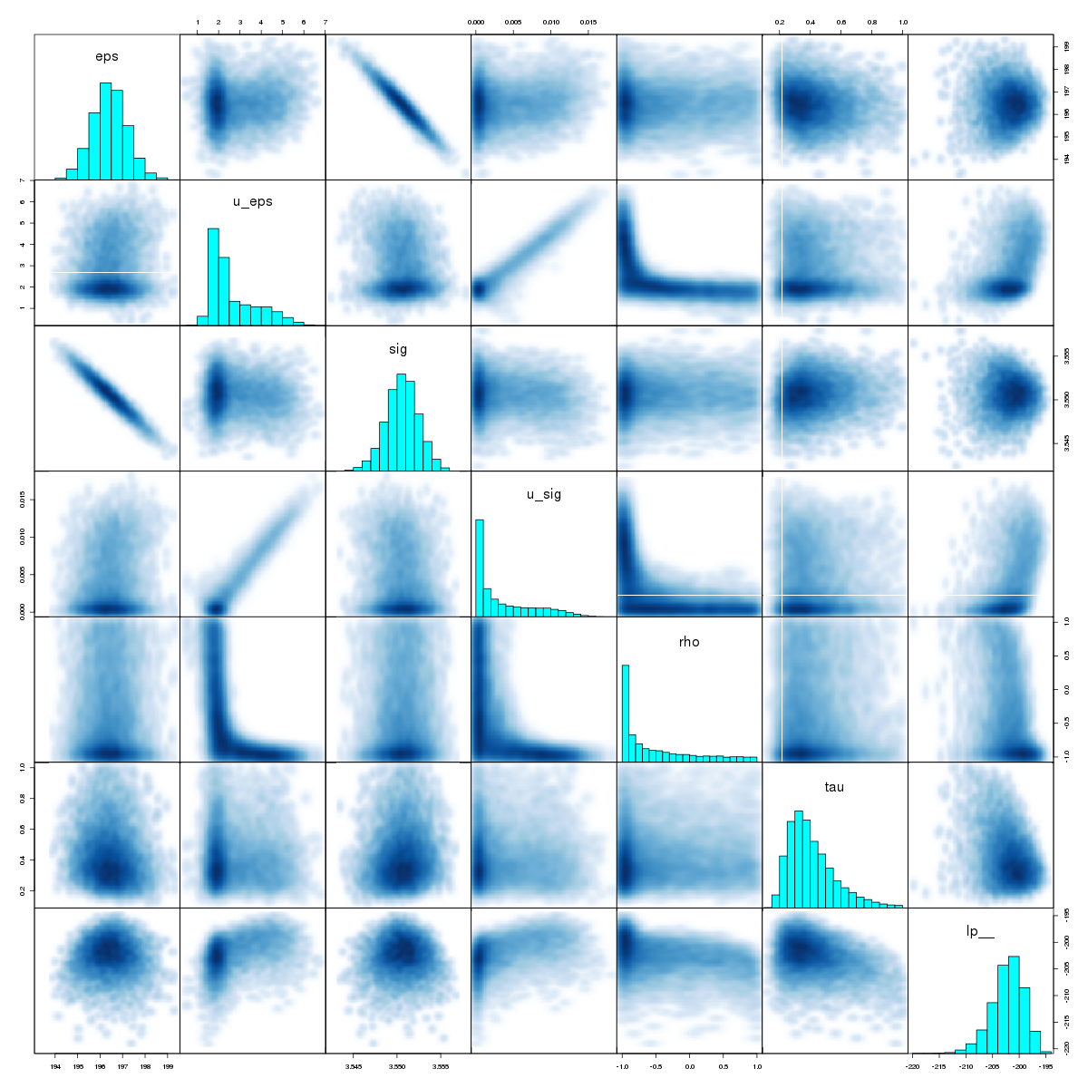
Figure 13: Pairs plot of parameters and log-posterior for the ABC-Shift method and Kr dataset.

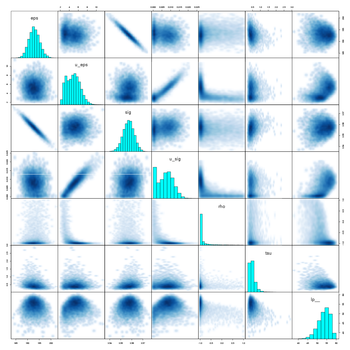
Figure 14: Pairs plot of parameters and log-posterior for the Margin-Shift method and Kr dataset.

References

- [1] Irikura KK, Johnson RD, Kacker RN. Uncertainty associated with virtual measurements from computational quantum chemistry models. Metrologia. 2004;41:369–375.
- [2] Two types of models are referred to in this study: physical (or knowledge) models used to make predictions of physico-chemical properties and statistical models used to calibrate the knowledge models. Most of the times, the simple term model will be used when there is no ambiguity. The same holds for the parameters of both types of models.
- [3] Cailliez F, Pernot P. Statistical approaches to forcefield calibration and prediction uncertainty of molecular simulations. J Chem Phys. 2011;134:054124.
- [4] Angelikopoulos P, Papadimitriou C, Koumoutsakos P. Bayesian uncertainty quantification and propagation in molecular dynamics simulations: A high performance computing framework. J Chem Phys. 2012;137:144103.
- [5] Cailliez F, Bourasseau A, Pernot P. Calibration of forcefields for molecular simulation: Sequential design of computer experiments for building cost-efficient kriging metamodels. J Comput Chem. 2013;35:130–149.
- [6] Angelikopoulos P, Papadimitriou C, Koumoutsakos P. Data Driven, Predictive Molecular Dynamics for Nanoscale Flow Simulations under Uncertainty. J Phys Chem B. 2013;117:14808–14816.
- [7] Chernatynskiy A, Phillpot SR, LeSar R. Uncertainty Quantification in Multiscale Simulation of Materials: A Prospective. Ann Rev Mat Res. 2013;43:157–182.
- [8] Hadjidoukas P, Angelikopoulos P, Papadimitriou C, Koumoutsakos P. 4U: A high performance computing framework for Bayesian uncertainty quantification of complex models. J Comput Phys. 2015;284:1–21.
- [9] Wu S, Angelikopoulos P, Papadimitriou C, Moser R, Koumoutsakos P. A hierarchical Bayesian framework for force field selection in molecular dynamics simulations. Phil Trans R Soc A. 2015;374:20150032.
- [10] Mortensen JJ, Kaasberg K, Frederiksen SL, Norksov JK, Sethna JP, Jacobsen KW. Bayesian error estimation in density functional theory. Phys Rev Lett. 2005;95:216401.
- [11] Wellendorff J, Lundgaard KT, Møgelhøj A, Petzold V, Landis DD, Nørskov JK, Bligaard T, Jacobsen KW. Density functionals for surface science: Exchange-correlation model development with Bayesian error estimation. Phys Rev B. 2012;85:235149.
- [12] Lejaeghere K, Speybroeck VV, Oost GV, Cottenier S. Error Estimates for Solid-State Density-Functional Theory Predictions: An Overview by Means of the Ground-State Elemental Crystals. Crit Rev Solid State Mater Sci. 2013;39:1–24.
- [13] Wellendorff J, Lundgaard KT, Jacobsen KW, Bligaard T. mBEEF: An accurate semi-local Bayesian error estimation density functional. J Chem Phys. 2014;140:144107.
- [14] Pernot P, Civalleri B, Presti D, Savin A. Prediction Uncertainty of Density Functional Approximations for Properties of Crystals with Cubic Symmetry. J Phys Chem A. 2015;119:5288–5304.
- [15] Pandey M, Jacobsen KW. Heats of formation of solids with error estimation: The mBEEF functional with and without fitted reference energies. Phys Rev B. 2015;91:235201.
- [16] Lejaeghere K, Vanduyfhuys L, Verstraelen T, Speybroeck VV, Cottenier S. Is the error on first-principles volume predictions absolute or relative? Comput Mater Sci. 2016;117:390–396.
- [17] Edwards DE, Zubarev DY, Packard A, Lester WA, Frenklach M. Interval Prediction of Molecular Properties in Parametrized Quantum Chemistry. Phys Rev Lett. 2014;112:253003.
- [18] Ruscic B. Uncertainty quantification in thermochemistry, benchmarking electronic structure computations, and Active Thermochemical Tables. Int J Quantum Chem. 2014;114:1097–1101.
- [19] Ulissi Z, Prasad V, Vlachos D. Effect of multiscale model uncertainty on identification of optimal catalyst properties. J Catal. 2011;281:339–344.
- [20] Medford AJ, Wellendorff J, Vojvodic A, Studt F, Abild-Pedersen F, Jacobsen KW, Bligaard T, Norskov JK. Assessing the reliability of calculated catalytic ammonia synthesis rates. Science. 2014;345:197–200.
- [21] Sutton JE, Guo W, Katsoulakis MA, Vlachos DG. Effects of correlated parameters and uncertainty in electronic-structure-based chemical kinetic modelling. Nat Chem. 2016;8:331–337.
- [22] Vasquez V, Whiting W. Incorporating uncertainty in chemical process design for environmental risk assessment. Environ Prog. 2004;23:315–328.
- [23] Androulakis I, Grenda J, Barckholtz T, Bozzelli J. Propagation of uncertainty in chemically activated systems. AIChE J. 2006;52:3246–3256.
- [24] Frenklach M. Transforming data into knowledge. Process Informatics for combustion chemistry. Proc Combust Inst. 2007;31:125–140.
- [25] Sheen DA, You X, Wang H, Løvas T. Spectral uncertainty quantification, propagation and optimization of a detailed kinetic model for ethylene combustion. Proc Combust Inst. 2009;32:535–542.
- [26] Russi T, Packard A, Frenklach M. Uncertainty quantification: Making predictions of complex reaction systems reliable. Chem Phys Lett. 2010;499:1–8.
- [27] Turányi T, Nagy T, Zsély IG, Cserháti M, Varga T, Szabó BT, Sedyó I, Kiss PT, Zempléni A, Curran HJ. Determination of rate parameters based on both direct and indirect measurements. Int J Chem Kinet. 2012;44:284–302.
- [28] Xing L, Li S, Wang Z, Yang B, Klippenstein SJ, Zhang F. Global uncertainty analysis for RRKM/master equation based kinetic predictions: A case study of ethanol decomposition. Combust Flame. 2015;162:3427–3436.
- [29] Wang H, Sheen DA. Combustion kinetic model uncertainty quantification, propagation and minimization. Prog Energy Combust Sci. 2015;47:1–31.
- [30] Cheung SH, Miki K, Prudencio E, Simmons C. Uncertainty quantification and robust predictive system analysis for high temperature kinetics of HCN/O2/Ar mixture. Chem Phys. 2016;475:136–152.
- [31] Frenklach M, Packard A, Garcia-Donato G, Paulo R, Sacks J. Comparison of Statistical and Deterministic Frameworks of Uncertainty Quantification. SIAM/ASA J Uncertain Quantif. 2016;4:875–901.
- [32] Kalyanaraman J, Kawajiri Y, Lively RP, Realff MJ. Uncertainty quantification via Bayesian inference using Sequential Monte Carlo methods for CO2 adsorption process. AIChE Journal. 2016;62:3352–3368.
- [33] BIPM, IEC, IFCC, ILAC, ISO, IUPAC, IUPAP, OIML. Evaluation of measurement data - Guide to the expression of uncertainty in measurement (GUM). Tech. Rep. 100:2008, Joint Committee for Guides in Metrology, JCGM. 2008.
- [34] BIPM, IEC, IFCC, ILAC, ISO, IUPAC, IUPAP, OIML. Evaluation of measurement data - Supplement 1 to the "Guide to the expression of uncertainty in measurement" - Propagation of distributions using a Monte Carlo method. Tech. Rep. 101:2008, Joint Committee for Guides in Metrology, JCGM. 2008.
- [35] de Rocquigny E, Devictor N, Tarantola S, eds. Uncertainty in Industrial Practice: A Guide to Quantitative Uncertainty Management. JOHN WILEY & SONS INC. 2008.
- [36] Williams CI, Feher M. The effect of numerical error on the reproducibility of molecular geometry optimizations. J Comput-Aided Mol Des. 2008;22:39–51.
- [37] Feher M, Williams CI. Numerical Errors and Chaotic Behavior in Docking Simulations. J Chem Inf Model. 2012;52:724–738.
- [38] Lira I. Combining inconsistent data from interlaboratory comparisons. Metrologia. 2007;44:415–421.
- [39] Toman B, Possolo A. Laboratory effects models for interlaboratory comparisons. Accredit Qual Assur. 2009;14:553–563.
- [40] Cox MG. The evaluation of key comparison data: determining the largest consistent subset. Metrologia. 2007;44:187–200.
- [41] Toman B. Bayesian Approaches to Calculating a Reference Value in Key Comparison Experiments. Technometrics. 2007;49:81–87.
- [42] Yuan Y, Khatibisepehr S, Huang B, Li Z. Bayesian method for simultaneous gross error detection and data reconciliation. AIChE Journal. 2015;61:3232–3248.
- [43] O’Hagan A. Bayesian inference with misspecified models: Inference about what? J Stat Plan Inference. 2013;143:1643–1648.
- [44] Scott AP, Radom L. Harmonic Vibrational Frequencies: An Evaluation of Hartree-Fock, Moller-Plesset and Quadratic Configuration Interaction and Density Functional Theory and and Semiempirical Scale Factors. J Phys Chem. 1996;100:16502–16513.
- [45] Pernot P, Cailliez F. Comment on "Uncertainties in scaling factors for ab initio vibrational zero-point energies" [J. Chem. Phys. 130, 114102 (2009)] and "Calibration sets and the accuracy of vibrational scaling factors: A case study with the X3LYP hybrid functional" [J. Chem. Phys. 133, 114109 (2010)]. J Chem Phys. 2011;134:167101.
- [46] Sargsyan K, Najm HN, Ghanem R. On the Statistical Calibration of Physical Models. Int J Chem Kinet. 2015;47:246–276.
- [47] Campbell K. Statistical calibration of computer simulations. Reliab Eng Syst Safe. 2006;91:1358–1363.
- [48] Oliver TA, Terejanu G, Simmons CS, Moser RD. Validating predictions of unobserved quantities. Comput Methods in Appl Mech Eng. 2015;283:1310–1335.
- [49] Pernot P. The parameters uncertainty inflation fallacy. SIAM/ASA J Uncertain Quantif. 2016;in review.
- [50] Gregory P. Bayesian Logical Data Analysis for the Physical Sciences. Cambridge University Press. 2005.
- [51] Gelman A, Carlin JB, Stern HS, Dunson DB, Vehtari A, Rubin DB. Bayesian Data Analysis. Chapman and Hall/CRC, 3rd ed. 2013.
- [52] McElreath R. Statistical Rethinking. Texts in Statistical Science. CRC Press. 2015.
- [53] Boldface type refers to vectors or matrices.
- [54] Birge RT. The Calculation of Errors by the Method of Least Squares. Phys Rev. 1932;40:207–227.
- [55] Kacker RN, Forbes A, Kessel R, Sommer KD. Classical and Bayesian interpretation of the Birge test of consistency and its generalized version for correlated results from interlaboratory evaluations. Metrologia. 2008;45:257–264.
- [56] Vehtari A, Ojanen J. A survey of Bayesian predictive methods for model assessment, selection and comparison. Statist Surv. 2012;6:142–228.
- [57] Gelman A, Lee D, Guo J. Stan: A Probabilistic Programming Language for Bayesian Inference and Optimization. J Educ Behav Stat. 2015;40:530–543.
- [58] R Core Team. R: A Language and Environment for Statistical Computing. R Foundation for Statistical Computing, Vienna, Austria. 2015.
- [59] Hoffman MD, Gelman A. The No-U-Turn Sampler: Adaptively Setting Path Lengths in Hamiltonian Monte Carlo. Journal of Machine Learning Research. 2014;15:1593–1623.
- [60] The uncertainty on the control variable is assumed to be negligible in all experiments.
- [61] Hibbert DB. Vocabulary of concepts and terms in chemometrics (IUPAC Recommendations 2016). Pure Appl Chem. 2016;88:407–443.
- [62] Transtrum MK, Machta BB, Sethna JP. Geometry of nonlinear least squares with applications to sloppy models and optimization. Phys Rev E. 2011;83:036701.
- [63] Arendt PD, Apley DW, Chen W. Quantification of Model Uncertainty: Calibration, Model Discrepancy, and Identifiability. J Mech Des. 2012;134:100908.
- [64] Brynjarsdóttir J, O’Hagan A. Learning about physical parameters: the importance of model discrepancy. Inverse Prob. 2014;30:114007.
- [65] Kennedy MC, O’Hagan A. Bayesian calibration of computer models. J R Stat Soc B. 2001;63:425–464.
- [66] Brown KS, Sethna JP. Statistical mechanical approaches to models with many poorly known parameters. Phys Rev E. 2003;68:021904.
- [67] Frederiksen SL, Jacobsen KW, Brown KS, Sethna JP. Bayesian Ensemble Approach to Error Estimation of Interatomic Potentials. Phys Rev Lett. 2004;93:165501.
- [68] Irikura KK, Johnson RD, Kacker RN. Uncertainties in Scaling Factors for ab Initio Vibrational Frequencies. J Phys Chem A. 2005;109:8430–8437.
- [69] Irikura KK, Johnson RD, Kacker RN, Kessel R. Uncertainties in scaling factors for ab initio vibrational zero-point energies. J Chem Phys. 2009;130:114102.
- [70] Johnson RD, Irikura KK, Kacker RN, Kessel R. Scaling Factors and Uncertainties for ab Initio Anharmonic Vibrational Frequencies. J Chem Theory Comput. 2010;6:2822–2828.
- [71] Weise K, Wöger W. Removing model and data non-conformity in measurement evaluation. Meas Sci Technol. 2000;11:1649–1658.
- [72] Bodnar O, Elster C. On the adjustment of inconsistent data using the Birge ratio. Metrologia. 2014;51:516–521.
- [73] Csilléry K, Blum MG, Gaggiotti OE, François O. Approximate Bayesian Computation (ABC) in practice. Trends Ecol Evol. 2010;25:410–418.
- [74] Sunnaker M, Busetto AG, Numminen E, Corander J, Foll M, Dessimoz C. Approximate Bayesian Computation. PLoS Comput Biol. 2013;9:e1002803.
- [75] Zarkova L. An isotropic intermolecular potential with temperature dependent effective parameters for heavy globular gases. Mol Phys. 1996;88:489–495.
- [76] Zarkova L. Viscosity, Second pVT-Virial Coefficient, and Diffusion of Pure and Mixed Small Alkanes CH4, C2H6, C3H8, n-C4H10, i-C4H10, n-C5H12, i-C5H12, and C(CH3)4 Calculated by Means of an Isotropic Temperature-Dependent Potential. I. Pure Alkanes. J Phys Chem Ref Data. 2006;35:1331.
- [77] Zarkova L, Hohm U. Effective ( n -6) Lennard-Jones Potentials with Temperature-Dependent Parameters Introduced for Accurate Calculation of Equilibrium and Transport Properties of Ethene, Propene, Butene, and Cyclopropane. J Chem Eng Data. 2009;54:1648–1655.
- [78] Bich E, Millat J, Vogel E. The viscosity and thermal conductivity of pure monatomic gases from their normal boiling point up to 5000 K in the limit of zero density and at 0.101325 MPa. J Phys Chem Ref Data. 1990;19:1289.
- [79] Kestin J, Ro S, Wakeham W. Viscosity of the Noble Gases in the Temperature Range 25-700 ∘C. J Chem Phys. 1972;56:4119–4124.
- [80] Vogel E. Präzisionsmessungen des Viskositätskoeffizienten von Stickstoff und den Edelgasen zwischen Raumtemperatur und 650 K. Ber Bunsenges Phys Chem. 1984;88:997–1002.
- [81] Dawe R, Smith E. Viscosity of the Inert Gases at High Temperatures. J Chem Phys. 1970;52:693–703.
- [82] Gough DW, Matthews GP, Smith EB. Viscosity of nitrogen and certain gaseous mixtures at low temperatures. J Chem Soc, Faraday Trans 1 F. 1976;72:645.
- [83] Goldblatt M, Guevara FA, McInteer BB. High Temperature Viscosity Ratios for Krypton. Phys Fluids. 1970;13:2873.