Cantor spectra of magnetic chain graphs

Abstract

We demonstrate a one-dimensional magnetic system can exhibit a Cantor-type spectrum using an example of a chain graph with $\delta$ coupling at the vertices exposed to a magnetic field perpendicular to the graph plane and varying along the chain. If the field grows linearly with an irrational slope, measured in terms of the flux through the loops of the chain, we demonstrate the character of the spectrum relating it to the almost Mathieu operator.

,

Keywords: quantum chain graph, magnetic field, almost Mathieu operator, Cantor spectrum

1 Introduction

The observation that spectra of quantum system may exhibit fractal properties was made first by Azbel [3] but it really caught the imagination when Hofstadter [16] made the structure visible; then it triggered a long and fruitful investigation of this phenomenon. On the mathematical side the question was translated into the analysis of the almost Mathieu equation which culminated recently in the proof of the “Ten Martini Problem” by Avila and Jitomirskaya [2]. On the physical side, the effect remained theoretical for a long time. Since the mentioned seminal papers, following an earlier work of Peierls [25] and Harper [15], the natural setting considered was a lattice in a homogeneous magnetic field because it provided the needed two length scales, generically incommensurable, from the lattice spacing and the cyclotron radius. The spectrum of the corresponding Hamiltonian has fractal properties as one can establish rigorously [6] by adapting deep results about appropriate difference operators [1, 2]. It was not easy to observe the effect, however, and the first experimental demonstration of such a spectral character was done instead in a microwave waveguide system with suitably placed obstacles simulating the almost Mathieu relation [19]. Only recently an experimental realization of the original concept was achieved using a graphene lattice [10, 26].

The aim of this note is to show that fractal spectra can arise also in magnetic systems extended in a single direction only under two conditions: the structure should have a nontrivial topology and the magnetic field should vary along it. We are going to demonstrate this claim using a simple example of a chain graph consisting of an array of identical rings connected at the vertices in the simplest nontrivial way known as the $\delta$ coupling and exposed to the magnetic field perpendicular to the graph plane the intensity of which increases linearly along the chain, with the slope $\alpha$ measured in terms of the number of the flux quanta through the ring. This is the decisive quantity. It turns out that when $\alpha$ is rational, the spectrum has a band-gap structure which allows for description in terms of the Floquet-Bloch theory. On the other hand, when $\alpha$ is irrational, the spectrum is a Cantor set, that is, a nowhere dense closed set without isolated points. The way to prove these results is to translate the original spectral problem into an equivalent one involving a suitable self-adjoint operator on $\ell^{2}(\mathbb{Z})$ which is a useful and well-known trick in the quantum graph theory, see e.g. [8, 12, 23]. As a result, in the rational case we rephrase the question as spectral analysis of a simple Laurent operator, while in the irrational case we reduce the problem to investigation of the almost Mathieu operator, for which the Cantor property of the spectrum is known as mentioned above [2].

Let us briefly describe the contents of the paper. In the next section we will define properly the operator that serves as the magnetic chain Hamiltonian. In Sec. 3 we explain our main technical tool, a duality between the quantum graph in question and an appropriate Jacobi operator, whose spectrum is described in Sec. 4. Finally, Sec. 5 contains our main result with some corollaries and a discussion; it is followed by a few concluding remarks.

2 Magnetic chain graph

Quantum graphs, which is a short name for Schrödinger operators the configuration space of which has the structure of a metric graph, are an important class of models in quantum physics. They are interesting both physically as models of various nanostructures, as well as from the viewpoint of their mathematical properties; we refer the reader to the recent monograph of Berkolaiko and Kuchment [5] for a thorough presentation and a rich bibliography. One important class is represented by magnetic quantum graphs, cf. for instance [18].

Let us describe the particular system we will be interested in. It is a metric graph $\Gamma$ consisting of an infinite linear chain of rings of unit radius, centred at equally spaced points laying at a straight line and touching their neighbours at the left and right. The vertices are parametrized by integers $\mathbb{Z}$ and both the upper edge $e_{j}^{U}$ and lower edge $e_{j}^{L}$ connecting the $j$-th vertex $v_{j}$ and $(j+1)$-th vertex $v_{j+1}$, which forms the $j$-th ring of the graph, are parametrized by intervals $(0,\pi)$ directed along the chain. Thus, if the initial vertex of an edge $e$ is denoted by $\iota e$ and the terminal vertex by $\tau e$, then $\iota e_{j}^{U}=\iota e_{j}^{L}=v_{j}$ and $\tau e_{j}^{U}=\tau e_{j}^{L}=v_{j+1}$. We assume that the system is exposed to a magnetic field perpendicular to the graph plane, which in contrast to [13] is not homogenerous but may vary along the chain. The Hamiltonian is the graph version of the magnetic Schrödinger operator acting as $\frac{1}{2m}\big{(}-i\hbar\nabla-\frac{e}{c}A\big{)}^{2}$ at each edge, where $A$ stands for the tangential component of the corresponding vector potential at a given point. However, it is known that in a magnetic chain there are only the fluxes through the loops that count, see [5, Corollary 2.6.3], and therefore we may, without loss of generality, choose a gauge in which the (tangent component of the) vector potential $A$ is constant at each particular ring; we denote by $A_{j}\in\mathbb{R}$ its value at the $j$-th ring and by $\boldsymbol{A}=\{A_{j}\}_{j\in\mathbb{Z}}$ the sequence of all such local vector potentials.

The state Hilbert space corresponding to a non-relativistic charged spinless particle confined to the graph $\Gamma$ is $L^{2}(\Gamma)$. For a function $\psi\in L^{2}(\Gamma)$ we further denote its components on the upper and lower semicircles $e_{j}^{U}$ and $e_{j}^{L}$ of the $j$-th ring by $\psi_{j}^{U}$ and $\psi_{j}^{L}$, respectively. The whole system is depicted in Figure 1.

Figure 1: Schematic depiction of the magnetic chain graph $\Gamma$.

Since the actual values of physical quantities will play no role in the discussion we employ the rational system of units putting $\hbar=2m=1$ and $\frac{e}{c}=1$. The Hamiltonian is then simply $-\Delta_{\gamma,\boldsymbol{A}}=-\mathcal{D}^{2}$, where $\mathcal{D}$ is the quasi-derivative which depends locally on the parametrisation of the edge and the magnetic field; specifically, on the upper and lower semicircles of the $j$-th chain ring, $\psi^{U}_{j}$ and $\psi^{L}_{j}$, it acts as

$$\mathcal{D}\psi^{U}_{j}=(\psi^{U}_{j})^{\prime}+iA_{j}\psi^{U}_{j}\quad\mathrm{and}\quad\mathcal{D}\psi^{L}_{j}=(\psi^{L}_{j})^{\prime}-iA_{j}\psi^{L}_{j},$$

respectively.

In order to make $-\Delta_{\gamma,\boldsymbol{A}}$ a well-defined self-adjoint operator we have to specify its domain which entails choosing the boundary conditions satisfied by the functions at the vertices of $\Gamma$, in physical terms this means to indicate the coupling between the rings. We choose for the latter the simplest nontrivial coupling commonly known as $\delta$. The domain $D(-\Delta_{\gamma,\boldsymbol{A}})$ then consists of all functions from the Sobolev space $H^{2}(\Gamma)$ satisfying at the graph vertices the conditions

$$\psi^{U}_{j}(0_{+})=\psi^{L}_{j}(0_{+})=\psi^{U}_{j-1}(\pi_{-})=\psi^{L}_{j-1}(\pi_{-}),$$ (1)

$$-\mathcal{D}\psi^{U}_{j-1}(\pi_{-})-\mathcal{D}\psi^{L}_{j-1}(\pi_{-})+\mathcal{D}\psi^{U}_{j}(0_{+})+\mathcal{D}\psi^{L}_{j}(0_{+})=\gamma\psi^{U}_{j}(0_{+})$$ (2)

for all $j\in\mathbb{Z}$, where $\gamma$ is the coupling constant and $\psi^{U}_{j}(0_{+})$ is the right limit of $\psi^{U}_{j}(x)$ at zero and $\psi^{U}_{j}(\pi_{-})$ is the left limit of $\psi^{U}_{j-1}(x)$ at the point $\pi$, etc. Note the different signs of the quasiderivative $\mathcal{D}$ at $0_{+}$ and $\pi_{-}$ which reflects the fact that the one-sided derivative at a vertex should be taken in the outgoing direction.

3 Duality with a discrete operator

In order to obtain the spectrum of $-\Delta_{\gamma,\boldsymbol{A}}$ we employ a particular kind of the duality mentioned in the introduction, relating it to the difference operator $L_{\boldsymbol{A}}$ which is a bounded self-adjoint operator on $\ell^{2}(\mathbb{Z})$ defined by

$$(L_{\boldsymbol{A}}\varphi)_{j}=2\cos(A_{j}\pi)\varphi_{j+1}+2\cos(A_{j-1}\pi)\varphi_{j-1}.$$ (3)

We employ the results obtained by K. Pankrashkin in [23, Section 2.3] using the boundary triple technique, see also [7].

To begin with, consider the local gauge transform $G$ given by

$$\big{(}G\psi^{U}_{j}\big{)}(x)=e^{-ixA_{j}}\psi^{U}_{j}(x)\quad\mathrm{and}\quad\big{(}G\psi^{L}_{j}\big{)}(x)=e^{ixA_{j}}\psi^{L}_{j}(x).$$

Using it, the operator $-\Delta_{\gamma,\boldsymbol{A}}$ is unitarily equivalent to the operator $H_{\gamma,\boldsymbol{A}}$ on $L^{2}(\Gamma)$ acting as

$$H_{\gamma,\boldsymbol{A}}\psi^{U}_{j}=-(\psi^{U}_{j})^{\prime\prime}\quad\mathrm{and}\quad H_{\gamma,\boldsymbol{A}}\psi^{L}_{j}=-(\psi^{L}_{j})^{\prime\prime}$$

with the domain $D(H_{\gamma,\boldsymbol{A}})$ consisting of the functions from $H^{2}(\Gamma)$ that obey the boundary conditions

$$\psi^{U}_{j}(0_{+})=\psi^{L}_{j}(0_{+})=e^{-i\pi A_{j-1}}\psi^{U}_{j-1}(\pi_{-})=e^{i\pi A_{j-1}}\psi^{L}_{j-1}(\pi_{-}),$$ (4)

$$-e^{-i\pi A_{j-1}}(\psi^{U}_{j-1})^{\prime}(\pi_{-})-e^{i\pi A_{j-1}}(\psi^{L}_{j-1})^{\prime}(\pi_{-})+(\psi^{U}_{j})^{\prime}(0_{+})+(\psi^{L}_{j})^{\prime}(0_{+})=\gamma\psi^{U}_{j}(0_{+}).$$ (5)

Consider next the solutions $s$ and $c$ of the differential equation $-y^{\prime\prime}-zy=0$ satisfying the boundary conditions

$$s(0_{+};z)=c^{\prime}(0_{+};z)=0\quad\mathrm{and}\quad s^{\prime}(0_{+};z)=c(0_{+};z)=1.$$

They are given explicitly by

$$s(x;z)=\cases{\frac{\sin(x\sqrt{z})}{\sqrt{z}}&for $z\neq 0$,\\ x&for $z=0$,}\quad\mathrm{and}\quad c(x;z)=\cos(x\sqrt{z}),$$

where $\sqrt{z}$ stands for the principal branch of the square root. For $z=k^{2}$ where $k\in\mathbb{N}$, $s(x;k^{2})$ is actually a solution on $(0,\pi)$ satisfying the Dirichlet boundary conditions. We denote the set of all such $z$ by $\sigma_{D}$, i.e. $\sigma_{D}=\{k^{2}|\,k\in\mathbb{N}\}$. The following proposition shows that all those points are actually eigenvalues of $H_{\gamma,\boldsymbol{A}}$ and thus also of $-\Delta_{\gamma,\boldsymbol{A}}$.

Proposition 3.1.

Let $k\in\mathbb{N}$ and $j\in\mathbb{Z}$ such that $A_{j}\in\mathbb{Z}$ or $A_{j-1},A_{j}\notin\mathbb{Z}$. Then there exists an eigenvector $\psi(k^{2},j)$ of $H_{\gamma,\boldsymbol{A}}$ corresponding to the eigenvalue $k^{2}$ which can be described as follows:

1. If $A_{j}\in\mathbb{Z}$ then

   $$\psi_{l}^{U}(x;k^{2},j)=\cases{s(x;k^{2})&for $l=j$,\\ 0&for $l\neq j$,}$$

   $$\psi_{l}^{L}(x;k^{2},j)=\cases{-s(x;k^{2})&for $l=j$,\\ 0&for $l\neq j$}$$

   for all $l\in\mathbb{Z}$.

2. If $A_{j-1},A_{j}\notin\mathbb{Z}$ then

   $$\psi_{l}^{U}(x;k^{2},j)= \cases{\phantom{-}\sin(A_{j}\pi)\cdot s(x;k^{2})&for $l=j-1$,\\ -\sin(A_{j-1}\pi)\cdot e^{i\pi A_{j}}\cdot s(x-\pi;k^{2})&for $l=j$,\\ \phantom{-}0&elsewhere,}$$

   $$\psi_{l}^{L}(x;k^{2},j)= \cases{-\sin(A_{j}\pi)\cdot s(x;k^{2})&for $l=j-1$,\\ \phantom{-}\sin(A_{j-1}\pi)\cdot e^{-i\pi A_{j}}\cdot s(x-\pi;k^{2})&for $l=j$,\\ \phantom{-}0&elsewhere}$$

   for all $l\in\mathbb{Z}$.

Proof.

In both cases the functions $\psi(k^{2},j)$ specified above clearly satisfy boundary conditions (4) and (5). ∎

Before we state the main spectral equivalence, we have to introduce another piece of notation. Let $H$ be a self adjoint operator and $B\subset\mathbb{R}$ a Borel set. By $H_{B}$ we denote the part of $H$ in $B$ referring to the spectral projection $\mathbbm{1}_{B}(H)$ of $H$ to the set $B$, in other words, $H_{B}=H\mathbbm{1}_{B}(H)$.

Theorem 3.2.

For any interval $J\subset\mathbb{R}\setminus\sigma_{D}$, the operator $(H_{\gamma,\boldsymbol{A}})_{J}$ is unitarily equivalent to the preimage $\eta^{(-1)}\big{(}(L_{\boldsymbol{A}})_{\eta(J)}\big{)}$, where

$$\eta(z)=\gamma s(\pi;z)+2c(\pi;z)+2s^{\prime}(\pi;z).$$

Proof.

The claim follows from Theorem 18 in [23] where both $\eta$ and the difference operator $L_{\boldsymbol{A}}$ are divided by four. ∎

Using the expressions for $s(x;z)$ and $c(x;z)$ we can write

$$\eta(z)=\cases{\gamma\,\frac{\sin\big{(}\pi\sqrt{z}\big{)}}{\sqrt{z}}+4\cos\big{(}\pi\sqrt{z}\big{)}&for $z\neq 0$,\\ \gamma\pi+4&for $z=0$.}$$ (6)

Thus, owing to the fact that $H_{\gamma,\boldsymbol{A}}$ is unitarily equivalent to $-\Delta_{\gamma,\boldsymbol{A}}$, the spectrum of $-\Delta_{\gamma,\boldsymbol{A}}$ is related to the spectrum of $L_{\boldsymbol{A}}$ via the preimage of $\sigma(L_{\boldsymbol{A}})$ under the entire function $\eta$. This means that, up to the discrete set $\{n^{2}|\,n\in\mathbb{N}\}$ of infinitely degenerate eigenvalues of $-\Delta_{\gamma,\boldsymbol{A}}$ which are described in Proposition 3.1, one has $\lambda\in\sigma(L_{\boldsymbol{A}})$ if and only if $\eta^{(-1)}\big{(}\{\lambda\}\big{)}=\{z\in\mathbb{R}|\,\eta(z)=\lambda\}\subset\sigma(-\Delta_{\gamma,\boldsymbol{A}})$. Moreover, $\lambda\in\sigma(L_{\boldsymbol{A}})$ is an eigenvalue if and only if points from $\eta^{(-1)}\big{(}\{\lambda\}\big{)}$ are eigenvalues and the same holds for the other parts of the spectrum, e.g. for the essential, absolutely continuous, and singular continuous spectral component.

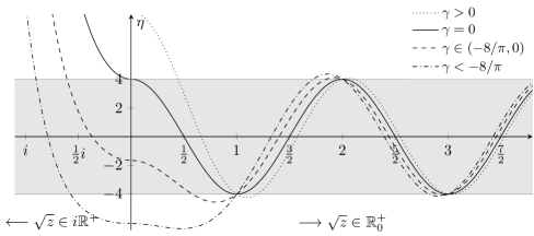
Figure 2: The influence of the parameter $\gamma$ on the behaviour of $\eta(z)$ which is plotted as a function of $\sqrt{z}$. On the right side of the vertical axis we plot the positive increasing values of $\sqrt{z}$ and on the left side we plot increasing values of the purely imaginary positive values of $\sqrt{z}$, i.e. of $\sqrt{z}=i\kappa$, $\kappa>0$.

Clearly, $\left\|L_{\boldsymbol{A}}\right\|\leq 4$, where $\left\|\cdot\right\|$ is the operator norm on $\ell^{2}(\mathbb{Z})$, and therefore $\sigma(L_{\boldsymbol{A}})\subset[-4,4]$. We are thus interested in the behaviour of $\eta$ when its values are inside the interval $[-4,4]$. This is shown in Figure 2. The function $\eta$ is continuous with the continuous derivative bounded in each interval $(x,\infty),x\in\mathbb{R}$, and it behaves essentially in the same way in each of the intervals $\big{[}n^{2},(n+1)^{2}\big{]},n\in\mathbb{N}$. Let $I_{n}:=\eta^{(-1)}\big{(}[-4,4]\big{)}\cap\big{(}n^{2},(n+1)^{2}\big{)}$ be the preimage of $[-4,4]$ restricted to $\big{(}n^{2},(n+1)^{2}\big{)}$. By inspecting the derivative of $\eta$, it is easy to check that $I_{n}$ is always an interval. Moreover, for $\gamma>0$ we have $I_{n}=\big{[}a_{n},(n+1)^{2}\big{)}$ where $n^{2}<a_{n}<(n+1)^{2}$. On the other hand, for $\gamma<0$ we have $I_{n}=(n^{2},b_{n}]$ where $n^{2}<b_{n}<(n+1)^{2}$. Finally, $I_{n}=\big{(}n^{2},(n+1)^{2}\big{)}$ holds for $\gamma=0$. Thus whenever $\gamma\neq 0$, the intervals $I_{n}$ are separated by a positive distance, i.e. there are gaps between parts of the spectrum.

For $z<1$, the behaviour of $\eta(z)$ is slightly different and much stronger influenced by the value of $\gamma$. If $\gamma>0$ then $\eta$ is decreasing on $(-\infty,1)$. If $-12/\pi\leq\gamma\leq 0$ then it is decreasing up to a certain point in $(0,1)$ and then increasing. Finally, if $\gamma<-12/\pi$ then $\eta$ is decreasing up to some point in $(-\infty,0)$ and then increasing. Let $I_{0}:=\eta^{(-1)}\big{(}[-4,4]\big{)}\cap\big{(}-\infty,1\big{)}$. It clearly follows that $I_{0}$ is again an interval. Since $\lim_{z\to-\infty}\eta(z)=\infty$, we obtain that for $\gamma>0$, $I_{0}=[a_{0},1)$ where $0<a_{0}<1$. For $\gamma=0$ we have $I_{0}=[0,1)$. For $-8/\pi<\gamma<0$, $I_{0}=[a_{0},b_{0}]$ where $a_{0}<0<b_{0}<1$. For $\gamma=-8/\pi$, $I_{0}=[a_{0},0]$ where $a_{0}<0$, and finally, for $\gamma<-8/\pi$, $I_{0}=[a_{0},b_{0}]$ where $a_{0}<b_{0}<0$. Note that $0\in I_{0}$ holds only when $\gamma\in[-8/\pi,0]$. These findings combined with Proposition 3.1 and Theorem 3.2 yield the following statement about the basic structure of the spectrum of $-\Delta_{\gamma,\boldsymbol{A}}$.

Proposition 3.3.

The spectrum of $-\Delta_{\gamma,\boldsymbol{A}}$ is bounded from below and can be decomposed into the discrete set $\sigma_{D}=\{n^{2}|\,n\in\mathbb{N}\}$ of infinitely degenerate eigenvalues and the part $\sigma_{L_{\boldsymbol{A}}}$ determined by the spectrum of $L_{\boldsymbol{A}}$, $\sigma(-\Delta_{\gamma,\boldsymbol{A}})=\sigma_{p}\cup\sigma_{L_{\boldsymbol{A}}}$, where $\sigma_{L_{\boldsymbol{A}}}$ can be written as the union

$$\sigma_{L_{\boldsymbol{A}}}=\bigcup_{n=0}^{\infty}\sigma_{n}$$

with $\sigma_{n}=\eta^{(-1)}\big{(}\sigma(L_{\boldsymbol{A}})\big{)}\cap I_{n}$ for $n\geq 0$, $I_{n}=\eta^{(-1)}\big{(}[-4,4]\big{)}\cap\big{(}n^{2},(n+1)^{2}\big{)}$ for $n>0$, and $I_{0}=\eta^{(-1)}\big{(}[-4,4]\big{)}\cap\big{(}-\infty,1\big{)}$.

When $\gamma\neq 0$, the spectrum has always gaps between the $\sigma_{n}$’s. For $\gamma>0$, the spectrum is positive. For $\gamma<-8\pi$, the spectrum has a negative part and does not contain zero. Finally, $0\in\sigma(-\Delta_{\gamma,\boldsymbol{A}})$ if and only if $\gamma\pi+4\in\sigma(L_{\boldsymbol{A}})$.

4 Spectrum in the general case

The main conclusion from the previous discussion is that in order to get a full picture of the spectrum of $-\Delta_{\gamma,\boldsymbol{A}}$ we need to investigate the spectrum of the bounded self-adjoint Jacobi operator $L_{\boldsymbol{A}}$. Spectral analysis of Jacobi operators is a well understood topic, see e.g. [31], and we can pick the tools suitable for our present case.

Denoting $a_{j}:=2\cos(A_{j}\pi)$ we can express the action of $L_{\boldsymbol{A}}$ as

$$(L_{\boldsymbol{A}}\varphi)_{j}=a_{j}\varphi_{j+1}+a_{j-1}\varphi_{j-1}$$

for any $\varphi\in\ell^{2}(\mathbb{Z})$. First thing to mention is that the spectrum of $L_{\boldsymbol{A}}$ does not depend on the signs of $a_{j}$. This follows from the fact that $L_{\boldsymbol{A}}$ is unitarily equivalent to $L_{\tilde{\boldsymbol{A}}}$ whenever $\left|a_{j}\right|=\left|\tilde{a}_{j}\right|$. It can be easily checked that the equivalence is mediated by the unitary operator $U_{\boldsymbol{A},\tilde{\boldsymbol{A}}}$, i.e. $L_{\tilde{\boldsymbol{A}}}=U_{\boldsymbol{A},\tilde{\boldsymbol{A}}}L_{\boldsymbol{A}}U_{\boldsymbol{A},\tilde{\boldsymbol{A}}}^{-1}$, defined by

$$\big{(}U_{\boldsymbol{A},\tilde{\boldsymbol{A}}}\varphi\big{)}_{j}=u_{j}\varphi_{j},$$

for any $\varphi\in\ell^{2}(\mathbb{Z})$, where

$$u_{j}=\cases{1&for $j=0$,\\ s_{j}s_{j-1}\ldots s_{2}s_{1}&for $j>0$,\\ s_{j}s_{j+1}\ldots s_{-2}s_{-1}&for $j<0$,}\quad\mathrm{and}\quad s_{j}=\cases{1&for $\tilde{a}_{j}=a_{j}$,\\ -1&otherwise.}$$

This unitary invariance can be used to find upper and lower bounds of the spectrum. By simple manipulations we get

$$\left\langle\varphi,L_{\boldsymbol{A}}\varphi\right\rangle=-\sum_{j\in\mathbb{Z}}a_{j}\left|\varphi_{j+1}-\varphi_{j}\right|^{2}+\sum_{j\in\mathbb{Z}}(a_{j-1}+a_{j})\left|\varphi_{j}\right|^{2}.$$

Let $\boldsymbol{A}^{+}$ be such that $a_{j}^{+}=\left|a_{j}\right|$, then we have

$$\left\langle\varphi,L_{\boldsymbol{A}}\varphi\right\rangle =\left\langle U_{\boldsymbol{A},\tilde{\boldsymbol{A}}}\varphi,L_{\boldsymbol{A}^{+}}U_{\boldsymbol{A},\tilde{\boldsymbol{A}}}\varphi\right\rangle\leq\sum_{j\in\mathbb{Z}}\big{(}\left|a_{j-1}\right|+\left|a_{j}\right|\big{)}\left|\big{(}U_{\boldsymbol{A},\tilde{\boldsymbol{A}}}\varphi\big{)}_{j}\right|^{2}$$

$$\leq\sup_{j\in\mathbb{Z}}c_{j}\left\|\varphi\right\|,$$

where

$$c_{j}=\left|a_{j-1}\right|+\left|a_{j}\right|=2\big{(}\left|\cos(A_{j-1}\pi)\right|+\left|\cos(A_{j}\pi)\right|\big{)}.$$

Similarly, using $\boldsymbol{A}^{-}$ such that $a_{j}^{-}=-\left|a_{j}\right|$, we get

$$\left\langle\varphi,L_{\boldsymbol{A}}\varphi\right\rangle=\left\langle U_{\boldsymbol{A},\tilde{\boldsymbol{A}}}\varphi,L_{\boldsymbol{A}^{-}}U_{\boldsymbol{A},\tilde{\boldsymbol{A}}}\varphi\right\rangle\geq-\sup_{j\in\mathbb{Z}}c_{j}\left\|\varphi\right\|,$$

which implies for the spectrum

$$\sigma(L_{\boldsymbol{A}})\subset[-\sup_{j\in\mathbb{Z}}c_{j},\sup_{j\in\mathbb{Z}}c_{j}].$$ (7)

Remark 4.1.

It follows from the previous bounds that if $\sup_{j\in\mathbb{Z}}c_{j}<4$, which means that all the pairs $A_{j-1},A_{j}$ are uniformly separated from pairs of integers, the gaps between the parts $\sigma_{n}$ of the spectrum of $-\Delta_{\gamma,\boldsymbol{A}}$ from Proposition 3.3 are always open and contain exactly one eigenvalue each.

Let us turn to the situation, when some $a_{j}$’s are equal to zero, which happens if the sequence $\{A_{j}\}$ contains half-integers. First we introduce some notation, putting

$$J_{0} :=\{j\in\mathbb{Z}\mid A_{j}+1/2\in\mathbb{Z}\},$$

$$J :=J_{0}\cup\big{(}\{-\infty\}\setminus\inf J_{0}\big{)}\cup\big{(}\{\infty\}\setminus\sup J_{0}\big{)},$$

i.e. $J$ contains $\infty$ whenever $J_{0}$ is bounded from above and $-\infty$ whenever $J_{0}$ is bounded from below. We say that $j,k\in J$ are neighbouring in $J$ if $j<k$ and there is no $i\in J$ such that $j<i<k$. For any $j,k\in J$ neighbouring in $J$ let $L_{j,k}$ be the restriction of $L_{\boldsymbol{A}}$ to $\{j+1,\ldots,k\}$. Clearly, $L_{j,k}$ is an operator on $\ell^{2}(\{j+1,\ldots,k\})$ given by

$$(L_{j,k}\varphi)_{i}=\cases{a_{j+1}\varphi_{j+2}&for $i=j+1$,\\ a_{j}\varphi_{j+1}+a_{j-1}\varphi_{j-1}&for $j+1<i<k$,\\ a_{k-1}\varphi_{k}&for $i=k$,}$$

where $a_{i}\neq 0$ for all $j<i<k$. This allows us to write the decomposition

$$L_{\boldsymbol{A}}=\bigoplus_{j,k\in J,\atop\mathrm{neighbouring\,in}\,J}L_{j,k}.$$

When $a_{j}\neq 0$ for all $j\in\mathbb{Z}$, then $J_{0}=\emptyset$, $J=\{-\infty,\infty\}$ and hence $L_{\boldsymbol{A}}=L_{-\infty,\infty}$.

Theorem 4.2.

Under the previous notation

$$\sigma(L_{\boldsymbol{A}})=\overline{\bigcup_{j,k\in J,\atop\mathrm{neighbouring\,in}\,J}\sigma(L_{j,k})}$$

and the essential spectrum of $L_{\boldsymbol{A}}$ is nonempty. If $j,k\in J_{0}$ then $L_{j,k}$ has a pure point spectrum containing $k-j$ different eigenvalues. If $j=-\infty$ or $k=\infty$ then the spectrum of $L_{j,k}$ has multiplicity at most two, that of the singular spectrum being one, and a nonempty essential part.

Proof.

The nonemptiness of the essential spectrum follows from boundedness of $L_{\boldsymbol{A}}$. When $j,k\in J_{0}$ the operator $L_{j,k}$ corresponds to a symmetric tridiagonal matrix $(k-j)\times(k-j)$ with nonzero upper and lower diagonals which implies that it has $k-j$ different eigenvalues. When $j=-\infty$ or $k=\infty$ then the assertion follows from Theorem 3.4, Lemma 3.6 in [31], and the boundedness of $L_{j,k}$. ∎

Note that the absolutely continuous spectrum of $L_{\boldsymbol{A}}$, which can be present only when $J_{0}$ is bounded from at least one side, can be further determined by the principle of subordinacy, see e.g. [31, Section 3.3].

Other interesting situation is the periodic one when there exists $N\in\mathbb{N}$ such that $A_{j}=A_{j+N}$ holds for all $j\in\mathbb{Z}$ or more generally, in view of the invariance of the spectrum w.r.t. the signs of $a_{j}$, when $\left|a_{j}\right|=\left|a_{j+N}\right|$ holds for all $j\in\mathbb{Z}$. If $a_{j}=0$, or equivalently $A_{j}+1/2\in\mathbb{Z}$ for some $j$, then the previous theorem implies that the spectrum is trivially given by a finite number of eigenvalues with infinite multiplicities. Otherwise, when $a_{j}\neq 0$ for all $j\in\mathbb{Z}$ one may apply Floquet-Bloch theory to show that the spectrum is purely absolutely continuous with a band-and-gap structure. The following assertion summarizes the result proven e.g. in [31, Sections 7.1 and 7.2].

Theorem 4.3.

Let $a_{j}\neq 0$ for all $j\in\mathbb{Z}$ and $\left|a_{j}\right|=\left|a_{j+N}\right|$ for some $N\in\mathbb{N}$ and all $j\in\mathbb{Z}$, i.e. $A_{j}+1/2\notin\mathbb{Z}$ and $\left|\cos(A_{j}\pi)\right|=\left|\cos(A_{j+N}\pi)\right|$, where $N$ is the smallest number with such property. Then the spectrum of $L_{\boldsymbol{A}}$ is purely absolutely continuous and consists of $N$ closed intervals possibly touching at the endpoints.

5 A linear field growth

Suppose now that $A_{j}=\alpha j+\theta$ holds for some $\alpha,\theta\in\mathbb{R}$ and every $j\in\mathbb{Z}$. We denote the corresponding operator $L_{\boldsymbol{A}}$ by $L_{\alpha,\theta}$, i.e.

$$(L_{\alpha,\theta}\varphi)_{j}=2\cos\big{(}\pi(\alpha j+\theta)\big{)}\varphi_{j+1}+2\cos\big{(}\pi(\alpha j-\alpha+\theta)\big{)}\varphi_{j-1}$$

for all $j\in\mathbb{Z}$. Properties of the spectrum of $L_{\alpha,\theta}$ are strongly influenced by number theoretic properties of $\alpha$ and $\theta$. If $\alpha$ is a rational number, $\alpha=p/q$, where $p$ and $q$ are relatively prime, then $L_{\alpha,\theta}$ is, according to the discussion in the previous section, periodic with the period $N=q$. Two distinct situations may occur depending on the value of $\theta$.

Theorem 5.1.

Assume that $\alpha=p/q$, where $p$ and $q$ are relatively prime. Then:

1. If $\alpha j+\theta+\frac{1}{2}\notin\mathbb{Z}$ for all $j=0,\ldots,q-1$, then $L_{\alpha,\theta}$ has purely absolutely continuous spectrum that consists of $q$ closed intervals possibly touching at the endpoints. In particular, $\sigma(L_{\alpha,\theta})=\big{[}-4\left|\cos(\pi\theta)\right|,4\left|\cos(\pi\theta)\right|\big{]}$ holds if $q=1$.

2. If $\alpha j+\theta+\frac{1}{2}\in\mathbb{Z}$ for some $j=0,\ldots,q-1$, then the spectrum of $L_{\alpha,\theta}$ is of pure point type consisting of $q$ distinct eigenvalues of infinite degeneracy. In particular, $\sigma(L_{\alpha,\theta})=\{0\}$ holds if $q=1$.

Proof.

Part (a) follows directly from Theorem 4.3. For $q=1$ corresponding to $\alpha\in\mathbb{Z}$ the spectrum may be calculated directly, see e.g. [31, Section 1.3].

In case (b) we may without loss of generality assume $\theta+\frac{1}{2}\in\mathbb{Z}$. Thus, $a_{j}=2\cos(A_{j}\pi)=0$ for $j\mathrm{\,mod\,}q=0$ and $a_{j}\neq 0$ otherwise. Hence, with the notation from the previous section, $J_{0}=J=q\mathbb{Z}$ and $L_{jq,(j+1)q}$ are the same for all $j\in\mathbb{Z}$. This together with Theorem 4.2 yields the assertion. If $q=1$ we have $\alpha\in\mathbb{Z}$ and from the assumption $\theta+\frac{1}{2}\in\mathbb{Z}$ it follows that $a_{j}=0$ holds for all $j\in\mathbb{Z}$, and consequently, $L_{\alpha,\theta}$ is a null operator. ∎

Remark 5.2.

Note that (a) occurs, for example, whenever $\theta$ is irrational.

On the other hand, if $\alpha\notin\mathbb{Q}$ the spectrum of $L_{\alpha,\theta}$ is closely related to the spectrum of the almost Mathieu operator $H_{\alpha,\lambda,\theta}$ in the critical situation, $\lambda=2$, which for any $\alpha,\lambda,\theta\in\mathbb{R}$ acts as

$$\big{(}H_{\alpha,\lambda,\theta}\varphi\big{)}_{j}=\varphi_{j+1}+\varphi_{j-1}+\lambda\cos(2\pi\alpha j+\theta)\varphi_{j}$$

for any $\varphi\in\ell^{2}(\mathbb{Z})$ and all $j\in\mathbb{Z}$. Recall that the almost Mathieu operator is one of the most studied discrete one-dimensional Schrödinger operator during several recent decades, see e.g. [20] for a review. The spectrum of $H_{\alpha,2,\theta}$ as a set when $\alpha$ is irrational has many interesting properties. First of all, it does not depend on $\theta$, see [4, 30]. Next, it is a Cantor set, i.e. the perfect nowhere dense set; this property is known as the “Ten Martini Problem”. The name of the challenge was coined by Simon [30], its proof was completed by Avila and Jitomirskaya in [2]. Moreover, the Lebesgue measure of the spectrum of $H_{\alpha,2,\theta}$ is zero, which is known as Aubry-André conjecture on the measure of the spectrum of the almost Mathieu operator, demonstrated finally by Avila and Krikorian in [1]. The picture arising from this survey can be described as follows.

Theorem 5.3.

For any $\alpha\notin\mathbb{Q}$, the spectrum of $H_{\alpha,2,\theta}$ does not depend on $\theta$ and it is a Cantor set of Lebesgue measure zero.

In order to reveal the relation between $L_{\alpha,\theta}$ and $H_{\alpha,2,\theta}$ we employ ideas from [29]. We start by introducing the abstract Rotation Algebra $A_{\alpha}$ which is a $C^{*}$ algebra generated by two unitary elements $u,v$ with the commutation relation

$$uv=e^{i2\pi\alpha}vu,$$

see also [11, 24, 9, 28] for more details. We can consider the representation $\pi_{\theta}$ generated by operators $U=\pi_{\theta}(u)$ and $V=\pi_{\theta}(v)$,

$$(U\varphi)_{j}:=\varphi_{j+1},\quad(V\varphi)_{j}:=e^{i2\pi\alpha j+\theta}\varphi_{j}.$$

Then the almost Mathieu operator coincides with the image of the element

$$h_{\alpha}=u+u^{-1}+v+v^{-1}\in A_{\alpha},$$

in other words, $H_{\alpha,2,\theta}=\pi_{\theta}(h_{\alpha})$. On the other hand, one can consider the representation $\pi^{\prime}_{\theta}$ generated by operators

$$(U\varphi)_{j}=e^{i\pi(\alpha j+\theta)}\varphi_{j+1},\quad(V\varphi)_{j}=e^{i\pi(\alpha(j-1)+\theta)}\varphi_{j-1}.$$

In this case we have $L_{\alpha,\theta}=\pi^{\prime}_{\theta}(h_{\alpha})$.

When $\alpha\notin\mathbb{Q}$, it can be checked that $A_{\alpha}$ is simple, see e.g. [11, 24, 27]. This implies that all its representations are faithful and thus they preserve the spectrum of $h_{\alpha}$, which is defined as a set of those complex $\lambda$ such that $h_{\alpha}-\lambda I$ is not invertible, see e.g. [24]. As a result, spectra of $L_{\alpha,\theta}$ and $H_{\alpha,2,\theta}$ as sets coincide,

$$\sigma(L_{\alpha,\theta})=\sigma(H_{\alpha,2,\theta}),$$ (8)

and are independent of $\theta$. This in combination with Theorem 5.3 proves the following assertion.

Theorem 5.4.

For any $\alpha\notin\mathbb{Q}$, the spectrum of $L_{\alpha,\theta}$ as a set does not depend on $\theta$ and it is a Cantor set of Lebesgue measure zero.

Remark 5.5.

Note that all the previous considerations are equally valid for any $A_{j}$ such that $\left|\cos(A_{j}\pi)\right|=\left|\cos\big{(}\pi(\alpha j+\theta)\big{)}\right|$ as a result of the invariance of the spectrum with respect to the signs of $a_{j}=\cos(A_{j}\pi)$ discussed in the previous section.

As for the original operator $-\Delta_{\gamma,\boldsymbol{A}}$, we may combine the previous observations to obtain the following theorem.

Theorem 5.6.

Let $A_{j}=\alpha j+\theta$ for some $\alpha,\theta\in\mathbb{R}$ and every $j\in\mathbb{Z}$. Then for the spectrum $\sigma(-\Delta_{\gamma,\boldsymbol{A}})$ the following holds:

1. If $\alpha,\theta\in\mathbb{Z}$ and $\gamma=0$, then $\sigma(-\Delta_{\gamma,\boldsymbol{A}})=\sigma_{ac}(-\Delta_{\gamma,\boldsymbol{A}})\cup\sigma_{pp}(-\Delta_{\gamma,\boldsymbol{A}})$ where $\sigma_{ac}(-\Delta_{\gamma,\boldsymbol{A}})=[0,\infty)$ and $\sigma_{pp}(-\Delta_{\gamma,\boldsymbol{A}})=\{n^{2}|n\in\mathbb{N}\}$ consists of infinitely degenerate eigenvalues.

2. If $\alpha=p/q$, where $p$ and $q$ are relatively prime, $\alpha j+\theta+\frac{1}{2}\notin\mathbb{Z}$ for all $j=0,\ldots,q-1$ and assumptions of part (a) do not hold, then $-\Delta_{\gamma,\boldsymbol{A}}$ has infinitely degenerate eigenvalues at the points of $\{n^{2}|\,n\in\mathbb{N}\}$ and an absolutely continuous part of the spectrum such that in each interval $(-\infty,1)$ and $\big{(}n^{2},(n+1)^{2}\big{)}$, $n\in\mathbb{N}$ it consists of $q$ closed intervals possibly touching at the endpoints.

3. If $\alpha=p/q$, where $p$ and $q$ are relatively prime, and $\alpha j+\theta+\frac{1}{2}\in\mathbb{Z}$ for some $j=0,\ldots,q-1$, then the spectrum $-\Delta_{\gamma,\boldsymbol{A}}$ is of pure point type and such that in each interval $(-\infty,1)$ and $\big{(}n^{2},(n+1)^{2}\big{)}$, $n\in\mathbb{N}$ there are exactly $q$ distinct eigenvalues and the remaining eigenvalues form the set $\{n^{2}|\,n\in\mathbb{N}\}$. All the eigenvalues are infinitely degenerate.

4. If $\alpha\notin\mathbb{Q}$, then $\sigma(-\Delta_{\gamma,\boldsymbol{A}})$ does not depend on $\theta$ and it is a disjoint union of the isolated-point family $\{n^{2}|\,n\in\mathbb{N}\}$ and Cantor sets, one inside each interval $(-\infty,1)$ and $\big{(}n^{2},(n+1)^{2}\big{)}$, $n\in\mathbb{N}$. Moreover, the overall Lebesgue measure of $\sigma(-\Delta_{\gamma,\boldsymbol{A}})$ is zero.

Proof.

For parts (a), (b) and (c) one uses Theorem 5.1, Proposition 3.3 and properties of function $\eta$ discussed before Proposition 3.3. The conclusion is implied by the bicontinuity of $\eta$ on each set $I_{n}$, $n\in\mathbb{N}$, and by the fact that in (b), (c) $\sigma(L_{\alpha,\theta})\subset(-4,4)$ follows from (7). Under the assumptions of (a), $\sigma(L_{\alpha,\theta})=[-4,4]$, and thus $\eta^{(-1)}\big{(}L_{\alpha,\theta}\big{)}=[0,\infty)$, see also Figure 2. The fact that the points $n^{2}$, $n\in\mathbb{N}$ are contained in $\sigma_{ac}(-\Delta_{\gamma,\boldsymbol{A}})$ results from the closeness of the absolutely continuous spectrum.

Finally, let us prove part (d). By Theorem 5.4, $\sigma(L_{\alpha,\theta})$ is a Cantor set with Lebesgue measure zero. From (7) it follows again that $\sigma(L_{\alpha,\theta})\subset(-4,4)$. Hence, since $\eta$ is bicontinuous in each set $I_{n}$, $n\geq 0$, the preimage $\sigma_{n}=f^{(-1)}\big{(}\sigma(L_{\alpha,\theta})\big{)}\cap I_{n}$ (using the notation from Proposition 3.3) is again a Cantor set contained in $(-\infty,1)$ for $n=0$ and in $\big{(}n^{2},(n+1)^{2}\big{)}$ for $n\in\mathbb{N}$, respectively. It is easy to see that the Lebesgue measure of $\sigma_{n}$ is zero for every $n\geq 0$ which implies that it is zero for the whole set. Now the sought assertion follows from Proposition 3.3. ∎

Remark 5.7.

It follows from the previous theorem that the eigenvalues $\{n^{2}|\,n\in\mathbb{N}\}$ are isolated points of the spectrum of $-\Delta_{\gamma,\boldsymbol{A}}$ if and only if $\gamma\neq 0$ or $\alpha\notin\mathbb{Z}$ or $\theta\notin\mathbb{Z}$.

Finally, we may apply the very recent result of Last and Shamis [21] which says that there is a dense $G_{\delta}$ set of $\alpha$’s, for which the Hausdorff dimension of the spectrum of $H_{\alpha,2,\theta}$ equals zero, $\dim_{H}\sigma(H_{\alpha,2,\theta})=0$, see e.g. [14, 22] for the definitions of Hausdorff measure and dimension. This result may be applied to the spectrum of $-\Delta_{\gamma,\boldsymbol{A}}$ as a consequence of the following proposition.

Proposition 5.8.

Let $A_{j}=\alpha j+\theta$ for some $\theta\in\mathbb{R}$, $\alpha\notin\mathbb{Q}$, and every $j\in\mathbb{Z}$. Then $\dim_{H}\sigma(-\Delta_{\gamma,\boldsymbol{A}})=\dim_{H}\sigma(L_{\alpha,\theta})$.

Proof.

It follows from (7) that $\sigma(L_{\alpha,\theta})\subset(-4,4)$. By the discussion preceding Proposition 3.3 and with the same notation, it follows that for any $n\geq 0$, $\sigma_{n}$ is contained in some closed subinterval $J_{n}$ of $I_{n}$. Moreover, for $n>0$ the function $\eta$ is bi-Lipschitz on $J_{n}$. Thus the inverse $(\eta|_{J_{n}})^{(-1)}$ of its restriction on $J_{n}$ is again bi-Lipschitz. Hence $\sigma_{n}$ is the image of $\sigma(L_{\alpha,\theta})$ under bi-Lipschitz function $(\eta|_{J_{n}})^{(-1)}$. It is a known fact, that bi-Lipschitz mappings preserve Hausdorff dimension, see e.g. [14, Corollary 2.4]. Hence $\dim_{H}(\sigma_{n})=\dim_{H}\sigma(L_{\alpha,\theta})$ for all $n>0$. For $n=0$ we may argue similarly for any closed set contained in $J_{0}\setminus\{0\}$. The point $0$ should be omitted since $\eta$ is not bi-Lipschitz on open sets containing zero. Let $H_{0}$ be a neighbourhood of $0$. Then $\sigma_{0}\setminus H_{0}$ is an image of $\sigma(L_{\alpha,\theta})\setminus\eta(H_{0})$ under a bi-Lipschitz function $(\eta|_{J_{0}})^{(-1)}$. Since $H_{0}$ was arbitrary, it follows that $\dim_{H}(\sigma_{0})=\dim_{H}\sigma(L_{\alpha,\theta})$. Finally, since countable sets have Hausdorff dimension zero, the countable stability, see e.g. Section 2.2 in [14], of Hausdorff measures yields the assertion. ∎

Thus, by [21, Theorem 1] and (8), one more assertion follows.

Corollary 5.9.

Let $A_{j}=\alpha j+\theta$ for some $\alpha,\theta\in\mathbb{R}$ and every $j\in\mathbb{Z}$. There exist a dense $G_{\delta}$ set $S$, such that for every $\alpha\in S$,

$$\dim_{H}\sigma(-\Delta_{\gamma,\boldsymbol{A}})=0$$

for all $\theta$.

6 Concluding remarks

To conclude, recall first that for any irrational $\alpha$ and (Lebesgue) almost all $\theta$ the spectrum of the almost Mathieu operator $H_{\alpha,2,\theta}$ is purely singularly continuous. This is a part of the more general Aubry-André conjecture proven by Jitomirskaya [17]. This fact motivates us to the question whether for any irrational $\alpha$ the spectrum of $L_{\alpha,\theta}$ has the same property, i.e. whether it is purely singularly continuous for Lebesgue a.e. $\theta$.

A deeper question concerns the physical meaning of the model that involves a magnetic field changing linearly along the chain. A philosophical answer could be, according the known quip of Bratelli and Robinson, that “validity of such idealizations is the heart and soul of theoretical physics and has the same fundamental significance as the reproducibility of experimental data”. On a more mundane level, one can note that the spectral behaviour will not change if the linear field is replaced by a quasiperiodic one which changes in a saw-tooth-like fashion as long as the jumps coincide with the graph vertices. This also opens an interesting question about the spectral form and type in case when the saw-tooth shape is replaced by another periodic or quasiperiodic function.

References

References

• [1] A. Avila, R. Krikorian: Reducibility or nonuniform hyperbolicity for quasiperiodic Schrödinger cocycles, Ann. Math., 164 (2006), 911–940.
• [2] A. Avila, S. Jitomirskaya: The Ten Martini Problem, Ann. Math., 170 (2009), 303–342.
• [3] M.Ya. Azbel: Energy spectrum of a conduction electron in a magnetic field, J. Exp. Theor. Phys 19 (1964), 634–645.
• [4] J. Avron, B. Simon: Almost periodic Schrödinger operators II. The integrated density of states, Duke Math. J., 50 (1983), 369–391.
• [5] G. Berkolaiko, P. Kuchment: Introduction to Quantum Graphs, Amer. Math. Soc., Providence, R.I., 2013.
• [6] J. Brüning, V. Geyler, K. Pankrashkin: Cantor and band spectra for periodic quantum graphs with magnetic fields., Commun. Math. Phys., 269 (2007), 87–105.
• [7] J. Brüning, V. Geyler, K. Pankrashkin: Spectra of self-adjoint extensions and applications to solvable Schrödinger operators, Rev. Math. Phys., 20 (2008), 1–70.
• [8] C. Cattaneo: The spectrum of the continuous Laplacian on a graph, Monatsh. Math., 124 (1997), 215–235.
• [9] M.-D. Choi, G.A. Elliott, N. Yui: Gauss polynomials and the rotation algebra, Invent. Math., 99 (1990), 225–246.
• [10] C.R. Dean et al.: Hofstadter’s butterfly and the fractal quantum Hall effect in moiré superlattices, Nature 497 (2013) 598–602.
• [11] E.G. Effros, F. Hahn: Locally compact transformation groups and $C^{*}$-algebras, Mem. AMS, vol. 73, Providence 1967.
• [12] P. Exner: A duality between Schrödinger operators on graphs and certain Jacobi matrices, Annales de l’I.H.P. Phys. théor., 66 (1997), 359–371.
• [13] P. Exner, S. Manko: Spectra of magnetic chain graphs: coupling constant perturbations, J. Phys. A: Math. Theor., 48 (2015), 125302.
• [14] K. Falconer : Fractal Geometry: Mathematical Foundations and Applications, 2nd ed., Wiley 2003.
• [15] P.G. Harper: The general motion of conduction electrons in a uniform magnetic field, with application to the diamagnetism of metals, Proc. Roy. Soc. A68 (1955), 879–892.
• [16] D.R. Hofstadter: Energy levels and wavefunctions of Bloch electrons in rational and irrational magnetic fields, Phys. Rev. B14 (1976), 2239–2249.
• [17] S.Ya. Jitomirskaya: Metal-insulator transition for the almost Mathieu operator, Ann. Math., 150 (1999), 1159–1175.
• [18] V. Kostrykin, R. Schrader: Quantum wires with magnetic fluxes, Commun. Math. Phys. 237 (2003), 161–179.
• [19] U. Kuhl, H.-J. Stöckmann: Microwave realization of the Hofstadter butterfly, Phys. Rev. Lett. 80 (1998), 3232–3235.
• [20] Y. Last: Spectral theory of Sturm-Liouville operators on infinite intervals: A review of recent developments, in Sturm-Liouville Theory (W.O. Amrein, A.M. Hinz, D.B. Pearson, eds.), Birkhäuser, Basel 2005; pp. 99–120.
• [21] Y. Last, M. Shamis: Zero Hausdorff dimension spectrum for the almost Mathieu operator, Commun. Math. Phys. 348 (2016), 729–750.
• [22] P. Mattila: Geometry of Sets and Measures in Euclidean Spaces, Cambridge University Press, 1995.
• [23] K. Pankrashkin: Unitary dimension reduction for a class of self-adjoint extensions with applications to graph-like structures, J. Math. Anal. Appl. 396 (2012), 640–655.
• [24] G.K. Pedersen: $C^{*}$-Algebras and Their Automorphism Groups, Academic Press, 1979.
• [25] R.E. Peierls: Zur Theorie des Diamagnetismus von Leitungselektronen, Zs. Phys. 80 (1933), 763–791.
• [26] L.A. Ponomarenko et al.: Cloning of Dirac fermions in graphene superlattices, Nature 497 (2013), 594–597.
• [27] S.C. Power: Simplicity of $C^{*}$-algebras of minimal dynamical systems, J. London Math. Soc., 3 (1978), 534–538.
• [28] M.A. Rieffel: $C^{*}$-algebras associated with irrational rotations, Pacific J. Math., 93 (1981), 415–429.
• [29] M.A. Shubin: Discrete magnetic Laplacian, Commun. Math. Phys., 164 (1994), 259–275.
• [30] B. Simon: Almost periodic Schrödinger operators: a review, Adv. Appl. Math., 3 (1982), 463–490.
• [31] G. Teschl: Jacobi Operators and Completely Integrable Nonlinear Lattices, Mathematical Surveys and Monographs, vol. 72, AMS, 2000.