Local environment effects on a charge carrier injected into an Ising chain

Abstract

We present numerically exact results for the spectral function of a single charge carrier that is injected into an Ising chain at finite temperature $T$. Both ferromagnetic and antiferromagnetic coupling between the Ising spins are considered. The interaction between the carrier and the Ising spins is assumed to be on-site and of Ising type, as well. We find that the carrier’s spectral function exhibits a distinctive fine structure of resonances that are due to the temporary entrapping of the carrier inside small magnetic domains. The connection to models of disordered binary alloys where similar effects can occur is explained. We use these results to construct an accurate (quasi)analytic approximation for low and medium-$T$ spectral functions.

I Introduction

Understanding the motion of charge carriers in magnetic backgrounds is a problem that appears in a variety of materials under a variety of circumstances. The magnetic order can be due to local or to itinerant moments; their magnetic order may be intrinsic or may be mediated by the charge carriers; the charge carriers may occupy the same or different bands from those giving rise to the magnetic background; at sufficiently low temperatures the background may order ferromagnetically (FM), antiferromagnetically (AFM), in more complicated patterns, or be frustrated; and so on and so forth.

One limit that has received a lot of attention is that of a single carrier evolving in a magnetic background of local moments that have long-range magnetic order in the absence of the carrier. If the carrier is injected into the band that hosts the local moments, its injection creates a hole in the magnetic background. Hopping of the hole changes the magnetic background as it corresponds to hopping in the opposite direction of a lattice spin. This situation is described by the so-called $t-J$ model which was first introduced by Anderson Anderson (1987) and then proposed as an effective model for cuprates by Zhang and Rice Zhang and Rice (1988); Dagotto (1994). Due to the possible connection to cuprates, such models have received a lot of attention.

This article, however, deals with a different case, where the carrier and the magnetic moments are hosted by different bands. Such a situation occurs, for instance, in FM semiconductors such as EuO and EuS and is described by the $s-f$ model Nolting (1979). In these materials the carrier is hosted in a wide $s$-band, whereas the local moments are hosted by a partially filled, strongly localized $f$-band. Here motion of the carrier does not necessarily modify the configuration of the magnetic background.

For these latter models, if the lattice spins have FM order at $T=0$, an exact solution for the carrier’s propagator exists. This is because the $z$-component of the total spin (carrier plus local moments) is conserved so the number of magnons that can be excited by the carrier is at most one (we assume that all spins are ${1\over 2}$). Starting from the FM state either no spin flip is possible (if the carrier has spin parallel to the background), or at most one magnon can be created (if the carrier has spin antiparallel to the background). The first case is trivial, and the second is simple enough to be solved analytically. The solution was first discussed in Ref. Shastry and Mattis, 1981 and then generalized to more complex lattices. Berciu and Sawatzky (2009) Analyses of the eigenstates and eigenenergies are also available.Henning et al. (2012); Nakano et al. (2012)

For an AFM background, on the other hand, an analytic solution is not known even at $T=0$ because the excitation of arbitrarily many magnons is now possible as the carrier can exchange the spins of any background pair with a spin-up and a spin-down. Combined with the generally very nontrivial nature of the AFM background wavefunction, this complicates matters exceedingly.

When trying to extend the FM solution to finite-$T$, one runs into somewhat similar problems because the carrier is now injected into a magnetic background which has a population of thermal magnons already present. Approximations for this case have been proposed (i) for medium to high-$T$, based on calculating moments of the Green’s function (GF) and fitting to limiting cases where the exact solution is known. The temperature enters via the magnetization $m$, which is assumed to be known and not to be affected by the carrier; Nolting et al. (2001) (ii) for weak and strong interactions between the carrier and the local moments, as well as fully FM ordered background and paramagnetic background, Kubo used the coherent potential approximation (CPA) to calculate the total density of states (DOS).Kubo (1974) CPA is a self-consistent approximation that assumes that the carrier propagates in an effective medium. Furthermore, Kubo uses the molecular field approximation for the interaction between local moments, thereby ignoring correlations; (iii) for very low-$T$, an approximation for the self-energy was obtained by us by limiting the states that enter the thermal average to one-magnon states.Möller and Berciu (2013) It shows unphysical features at higher temperatures where higher energy states become relevant.

None of these approaches includes fully the effects of the local environment on the carrier. In this article we try to answer the question of what role, if any, is played by the local environment. Is there a class of configurations that contributes more than others? How does an AFM ordered environment compare to a FM ordered one, and are there any similarities between the two? Answering such questions is crucial for the development of a better understanding (and hopefully better approximations) for the finite-$T$ spectral weight of the carrier.

Our approach is to study a simplified model which allows us to obtain the first (to the best of our knowledge) finite-$T$ exact numerical results in the thermodynamic limit. These teach us valuable lessons about the physics of this simpler problem; some of these are relevant for more complex models, too. The simplification consists in neglecting all spin-flip processes, i.e. assuming that all interactions between the lattice spins, and between them and the carrier, are Ising-like. While the $T=0$ behavior of this model is trivial, we find that it produces rich physics at finite-$T$, which needs to be understood before considering the additional complications introduced by allowing spin-flip processes.

Apart from making an exact solution possible, this simple model also allows us to consider both FM and AFM backgrounds on equal footing, which is not possible in general. Interestingly, we find considerable similarities between the results for the two cases, which we are able to explain as being due to similarities between the local background configurations that control the (at least low and medium-$T$) carrier dynamics. We then use these insights to construct an analytical approximation which accurately reproduces the features of the exact solution in the range of low to medium temperatures.

By ignoring spin-flip processes, we create a situation that is in some ways similar to that of disorder binary alloys of the type A_xB_1-x. A carrier in the conduction band of such an alloy experiences a different on-site energy if it sits on an A or a B site. In our model the on-site carrier energy is $\pm J_{0}$, depending on whether the local spin at that site points up or down. Thus, any configurations of the alloy can be exactly mapped into a spin configuration of the magnetic background.

These binary alloys have been extensively studied. An exact numerical solution can be obtained for the disorder-averaged GFs, as pointed out by SchmidtSchmidt (1957) and Dyson.Dyson (1953) It was used for numerical studies of the phonon DOS Dean (1972) and the DOS of carriers in the conduction band.Alben et al. (1975); Economou (2006) Many approximations have been proposed, the most well-known and used being the CPA.Soven (1967) Diagrammatic expansions of the self-energy have been developed by several authors, see for instance Refs. Yonezawa, 1968; Nickel and Krumhansl, 1971; Butler and Kohn, 1970, but were shown to result in non-analytic behavior and thus unphysical GFs.Nickel and Butler (1973) Later this problem was resolved by a careful consideration of which diagrams to sum.Mills and Ratanavararaksa (1978)

This knowledge cannot be directly used in our problem, despite the similarities between the models, because for binary alloys one performs a disorder average whereas we do a thermal average. The disorder average keeps the concentration $x$ fixed; all configurations consistent with it are equally likely (one generally ignores correlations in the disorder), all the others are forbidden. In contrast, a thermal average includes all possible configurations but with a Boltzmann factor that controls the extent of spin-spin correlations. These correlations are key, as no magnetic order can exist in their absence. The problems also have different symmetry properties. Our problem is truly translationally invariant, whereas for binary alloys translational invariance is only restored by averaging over all possible disorder configurations. For example, while all eigenstates are localized in a 1D disordered alloy model, the eigenstates of our model remain extended at any $T$. Despite these differences, there are similarities between the resulting spectral weights which help us understand our results, as discussed below.

This article is organized as follows. Section II presents the model and Section III describes the method by which we calculate the GF. Results are discussed in Section IV for a 1D chain, although the method can be trivially extended to higher dimension. We also present here the analytic approximation we propose for low and medium temperatures. The concluding remarks are in Section V.

II Model

Consider a single spin-${1\over 2}$ charge carrier which interacts with a chain of Ising spins, also of magnitude ${1\over 2}$. Note that the exact method that we use can be generalized straightforwardly to higher dimensions. The advantage of 1D chains (apart from speed of computations) is that a host of analytic results are available for the undoped case. We therefore limit ourselves here to Ising chains with periodic boundary conditions after $N\rightarrow\infty$ sites. The $n^{\text{th}}$ site is located at $R_{n}=na$, and we set $a=1$.

The exchange between lattice spins is Ising-like:

$$\hat{H}_{\text{I}}=-J\sum_{i}\hat{\sigma}_{i}\hat{\sigma}_{i+1}-h\sum_{i}\hat{\sigma}_{i},$$ (1)

and is FM ($J>0$) or AFM ($J<0$). The second term describes the effect of an external magnetic field $h$. The spin operator at site $i$ is $S_{i}^{z}={1\over 2}\hat{\sigma}_{i}$, with the prefactors absorbed into the coupling constants. The eigenstates $\hat{H}_{\text{I}}|\{\sigma\}\rangle=E_{I}(\{\sigma\})|\{\sigma\}\rangle$ are described by the set $\{\sigma\}\equiv\{\sigma_{1},\sigma_{2},\dots,\sigma_{N}\}$ of eigenvalues $\sigma_{i}=\pm 1$ of each spin, and $E_{I}(\{\sigma\})=-J\sum_{i}\sigma_{i}\sigma_{i+1}-h\sum_{i}\sigma_{i}$ is the eigenenergy.

The kinetic energy of the carrier is described by a tight-binding model

$$\hat{T}=-t\sum_{i,\sigma}\left(c_{i,\sigma}^{\dagger}c_{i+1,\sigma}+\text{h.c.}\right)=\sum_{k,\sigma}\varepsilon(k)c_{k,\sigma}^{\dagger}c_{k,\sigma},$$ (2)

where $c_{i,\sigma}^{\dagger}$ is the creation operator of a spin-$\sigma$ carrier at site $i$. The creation operator in momentum-space is $c_{k,\sigma}^{\dagger}={1\over\sqrt{N}}\sum_{n}\mathrm{e}^{ikR_{n}}c_{n,\sigma}^{\dagger}$, and $\varepsilon(k)=-2t\cos(k)$.

The exchange between the carrier and the lattice spins is also of Ising type:

$$\hat{H}_{\text{exc}}=J_{0}\sum_{i,\sigma}\sigma c_{i,\sigma}^{\dagger}c_{i,\sigma}\hat{\sigma}_{i},$$ (3)

where again a factor $1/4$ is absorbed into $J_{0}$. Since no spin-flips are allowed in this model, from now on we assume without loss of generality that the carrier has spin-up, $\sigma=\uparrow$, and not write it explicitly. We also set $J_{0}>0$. Results for a spin-down carrier are obtained from these by switching $J_{0}\rightarrow-J_{0}$.

For the undoped Ising chain, an exact solution at finite-$T$ is possible and reviewed in the appendix. Note that a 1D chain has long-range magnetic order only at $T=0$. We can, however, mimic a finite-$T$ ordered state by turning on the magnetic field $h$. This leads to a finite correlation independent of the distance between spins.

III Method

We want to calculate the finite-$T$ retarded single-particle GF, which in the time-domain is defined as:

$$G(k,\tau)=-i\theta(\tau)\left\langle c_{k}(\tau)c_{k}^{\dagger}(0)\right\rangle_{T}$$ (4)

where the operator $c_{k}(\tau)=\mathrm{e}^{i\hat{H}\tau}c_{k}\mathrm{e}^{-i\hat{H}\tau}$ is in the Heisenberg picture. Furthermore $\left\langle\dots\right\rangle_{T}=\frac{1}{Z}\sum_{\{\sigma\}}\langle\{\sigma\}|\mathrm{e}^{-\beta E_{I}(\{\sigma\})}\dots|\{\sigma\}\rangle$ is the thermal average and $\beta=1/(k_{B}T)$. From now on we set $\hbar=1,k_{B}=1$.

It needs to be pointed out that the temperature dependence in Eq. (4) is solely controlled by $\hat{H}_{\text{I}}$: we inject the carrier into the otherwise undoped Ising chain, which at a given $T$ is described by a density matrix $\hat{\rho}_{I}=\mathrm{e}^{-\beta\hat{H}_{\text{I}}}/Z$. In other words, this formulation is for a canonical ensemble with a conserved carrier number, not the usual grand-canonical formulation.

It is convenient to work in the frequency-domain. We Fourier transform $G(k,\omega)=\int_{\infty}^{-\infty}\mathrm{d}\tau\ \mathrm{e}^{i\omega\tau}G(k,\tau)$ which yields:

$$G(k,\omega)=\left\langle c_{k}\hat{G}(\omega+\hat{H}_{I})c_{k}^{\dagger}\right\rangle_{T},$$ (5)

where $\hat{G}(\omega)=(\omega-\hat{H}+i\eta)^{-1}$ is the resolvent of $\hat{H}$. The small, real quantity $\eta>0$ ensures retardation and sets a finite carrier lifetime $1/\eta$. Note that the argument of the resolvent in Eq. (5) is shifted by $\hat{H}_{I}$. This means that the energy is measured from that of the Ising chain at the time of injection. This becomes clear when using a Lehmann representation by projecting on the one-carrier eigenstates $\hat{H}|\psi_{n}\rangle=E_{n}|\psi_{n}\rangle$:

$$G(k,\omega)=\sum_{n}\sum_{\{\sigma\}}\frac{\mathrm{e}^{-\beta E_{I}(\{\sigma\})}}{Z}\frac{\langle\{\sigma\}|c_{k}|\psi_{n}\rangle\langle\psi_{n}|c_{k}^{\dagger}|\{\sigma\}\rangle}{\omega+E_{I}(\{\sigma\})-E_{n}+i\eta}$$ (6)

$G(k,\omega)$ has poles at energies $\omega=E_{n}-E_{I}(\{\sigma\})$ that measure the change in total energy due to the carrier’s injection. The weights correspond to the overlap between the true eigenstates $|\psi_{n}\rangle$ and the free-carrier states $c_{k}^{\dagger}|\{\sigma\}\rangle$.

For any configuration $\{\sigma\}$, the contribution to the thermal average can be evaluated using continued fractions.Berciu and Cook (2010) First, we need to shift to the real-space representation. Making use of the translational invariance we then obtain

$$G(k,\omega)=\sum_{n}\mathrm{e}^{ikR_{n}}\left\langle g_{0,n}(\omega,\{\sigma\})\right\rangle_{T},$$ (7)

where we define:

$$g_{m,n}(\omega,\{\sigma\})=\langle\{\sigma\}|c_{m}\hat{G}(\omega+\hat{H}_{I})c_{n}^{\dagger}|\{\sigma\}\rangle.$$ (8)

Physically $g_{m,n}(\omega,\{\sigma\})$ is related to the probability that the carrier is injected at site $n$ and propagates to site $m$. For any state $\{\sigma\}$ (except the fully ordered ones) the translational invariance is broken, $g_{m,n}(\omega,\{\sigma\})\neq g_{0,n-m}(\omega,\{\sigma\})$. This symmetry is only restored by the ensemble average, which then leads to Eq. (7).

To obtain the GF equations of motion (EOM) we use Dyson’s identity $\hat{G}(\omega)=\hat{G}_{0}(\omega)+\hat{G}(\omega)\hat{V}\hat{G}_{0}(\omega)$ where $\hat{H}=\hat{H}_{0}+\hat{V}$ and $\hat{G}_{0}(\omega)$ is the resolvent for $\hat{H}_{0}$. Choosing $\hat{H}_{0}=\hat{H}_{I}+\hat{H}_{\text{exc}}$, we find:

$$g_{0,n}(\omega,\{\sigma\})= G_{0}(\omega-J_{0}\sigma_{n})\left(\delta_{0,n}-tg_{0,n-1}(\omega,\{\sigma\})\right.$$

$$\left.-tg_{0,n+1}(\omega,\{\sigma\})\right),$$ (9)

where $G_{0}(\omega)=(\omega+i\eta)^{-1}$. Since the EOM do not change the values of $\omega$ and $\{\sigma\}$, to shorten notation we do not write them explicitly in the following.

The EOM are solved with the ansatz Berciu and Cook (2010) $g_{0,n}=A_{n}g_{0,n-1}$ for $n>0$ and $g_{0,n}=B_{-n}g_{0,n+1}$ for $n<0$ ($N\rightarrow\infty$ is assumed and implemented as explained below). Then

$$A_{n}=\frac{-tG_{0}(\omega-J_{0}\sigma_{n})}{1+tG_{0}(\omega-J_{0}\sigma_{n})A_{n+1}},$$ (10)

and similarly for $B_{n}$. We now introduce a cutoff $M_{c}\gg 1$ at which we truncate these relations by setting $A_{M_{c}+1}=B_{M_{c}+1}=0$. The justification is provided by the finite lifetime $1/\eta$ of the carrier, which prevents it from propagating arbitrarily far from its injection site. As a result $g_{0,n}$, which measures the amplitude of probability that the carrier propagates between sites $n$ and 0, must vanish for sufficiently large $|n|$.Berciu and Cook (2010)

It is then straightforward to calculate all $A_{1},\dots,A_{M_{c}}$ and $B_{1},\dots,B_{M_{c}}$ for the configuration $\{\sigma\}$ and a given $\omega$, to find:

$$g_{0,0}=\frac{1}{\omega-J_{0}\sigma_{0}+t(A_{1}+B_{1})}$$ (11)

$$g_{0,n}=A_{M_{c}}\dots A_{1}g_{0,0},\mbox{ if }n>0$$ (12)

$$g_{0,-n}=B_{M_{c}}\dots B_{1}g_{0,0},\mbox{ if }n<0.$$ (13)

Let us now discuss the cutoff $M_{c}$ in more detail. In practice $M_{c}$ is increased until convergence is reached. Since $g_{0,0}$ for the fully ordered configuration is known analytically, it can be used to verify the convergence.

We need to have $M_{c}\ll N/2$, otherwise the carrier may travel between sites $n$ and 0 on both sides of the closed loop, which is at odds with the ansatz chosen above. This condition is automatically satisfied if $N\rightarrow\infty$. To take this limit, we note that $g_{0,n}$ only depend on the spins $\sigma_{-M_{c}},\sigma_{-M_{c}+1},\ \dots\ ,\sigma_{M_{c}}$. We make use of this by splitting the full set $\{\sigma\}$ into the set $\{M_{c}\}$ containing just the aforementioned spins, and the complementary set $\{M_{c}\}^{C}$. The energy of the Ising chain is also split: $E_{I}(\{\sigma\})=E_{I}(\{M_{c}\})+E_{I}(\{M_{c}\}^{C},\sigma_{-M_{c}},\sigma_{M_{c}})$, where

$$E_{I}(\{M_{c}\})=-J\sum_{n=-M_{c}}^{M_{c}-1}\sigma_{n}\sigma_{n+1}-h\sum_{n=-M_{c}}^{M_{c}}\sigma_{n}$$ (14)

and $E_{I}(\{M_{c}\}^{C},\sigma_{-Mc},\sigma_{M_{c}})$ contains the energy of all other bonds and spins, including the “boundary” bonds $\sigma_{M_{c}}\sigma_{M_{c}+1}$ and $\sigma_{-M_{c}-1}\sigma_{-M_{c}}$. This is why it also depends on $\sigma_{\pm M_{c}}$, not just on the $\{M_{c}\}^{C}$ spins.

Eq. (7) can then be rewritten as:

$$G(k,\omega)= \sum_{n}\mathrm{e}^{ikR_{n}}\sum_{\{M_{c}\}}\frac{\mathrm{e}^{-\beta E_{I}(\{M_{c}\})}}{Z}g_{0,n}(\omega,\{M_{c}\})$$

$$\times Z_{\text{bath}}(\beta,\sigma_{-M_{c}},\sigma_{M_{c}}),$$ (15)

where

$$Z_{\text{bath}}(\beta,\sigma_{-M_{c}},\sigma_{M_{c}})=\sum_{\{M_{c}\}^{C}}\mathrm{e}^{-\beta E_{I}(\{M_{c}\}^{C},\sigma_{-Mc},\sigma_{M_{c}})}.$$ (16)

$Z_{\text{bath}}$ is the partition function of the complementary set of spins $\{M_{c}\}^{C}$, for set values of its “boundary” spins $\sigma_{-M_{c}}$ and $\sigma_{M_{c}}$. Using transfer matrices (see Appendix for details), we find that:

$$Z_{\text{bath}}(\beta,\sigma_{M_{c}},\sigma_{-M_{c}})=\left(\mathcal{T}^{N-2M_{c}}\right)_{\sigma_{M_{c}},\sigma_{-M_{c}}}.$$ (17)

Thus, $\lim_{N\rightarrow\infty}Z_{\text{bath}}(\beta,\sigma_{M_{c}},\sigma_{-M_{c}})/Z$ is known analytically. The average in Eq. (15) now involves only the spins $\{M_{c}\}$ in the chain sector that can be explored by the carrier within its finite lifetime $1/\eta$. Effectively, the rest of the infinite chain is treated as a bath that is integrated out analytically. We use the Metropolis algorithm to estimate the sum over the $\{M_{c}\}$ set. The results are discussed next.

IV Results

IV.1 T=0 result

We begin by briefly reviewing the $T=0$ solution which can be calculated exactly and serves as a useful reference.

For FM coupling $J>0$, at $T=0$ all Ising spins point either up or down, $m=\pm 1$. Then $\hat{H}_{\text{exc}}$ simply shifts the energy of the carrier by $J_{0}m$: $E_{m}^{\text{FM}}(k)=\varepsilon_{k}+J_{0}m$. As $T\rightarrow 0$ and for $h=0$, an infinite chain will arbitrarily choose as its ground state one of these two possible FM configurations. One can control which configuration is chosen by cooling the system in a small magnetic field, which is then switched off. However, as long as the temperature is not exactly zero and if $h=0$, then the presence of large domains with opposite order is possible, especially in 1D. If the carrier is injected into one of these large domains it is unable to leave it within its finite lifetime $1/\eta$. Consequently as $T\rightarrow 0$ and for $h=0$ we expect to see contributions from both subspaces $m<0$ and $m>0$, and the GF becomes:

$$G^{\text{FM}}(k,\omega)=\frac{1}{2}\left(\frac{1}{\omega-E^{\text{FM}}_{+}+i\eta}+\frac{1}{\omega-E^{\text{FM}}_{-}+i\eta}\right).$$ (18)

For AFM coupling there are also two possible ground states: either all spins of the even sublattice point up and all spins of the odd sublattice point down, or vice versa. The doubling of the unit cell results in the appearance of two bands in the reduced Brillouin zone $(-\pi/2,\pi/2]$, with energies $E^{\text{AFM}}_{\pm}(k)=\pm\sqrt{J_{0}^{2}+\varepsilon_{k}^{2}}$. Averaging over both contributions for the reasons discussed above, the $T\rightarrow 0,h=0$ GF is found to be:

$$G^{\text{AFM}}(k,\omega)=\frac{\omega+\varepsilon_{k}+i\eta}{(\omega-E^{\text{AFM}}_{+}+i\eta)(\omega-E^{\text{AFM}}_{-}+i\eta)}$$ (19)

for any $k\in(-\pi,\pi]$.

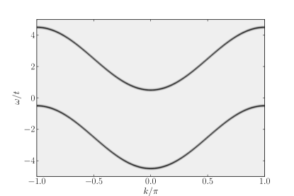
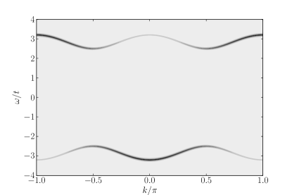
Figure 1: Contour plots of the $T=0$ spectral functions for FM (top) and AFM (bottom) coupling, for $|J|/t=0.5,\ J_{0}/t=2.5,\ h=0,\ \eta/t=0.04$.

Contour plots of the spectral function $A(k,\omega)=-\frac{1}{\pi}\text{Im}G(k,\omega)$ for these GFs are shown in Fig. 1. As expected from applying the Lehmann representation, Eq. (6), to these GFs, the spectrum consists of two bands for both FM and AFM coupling. For FM coupling, the bands have bandwidths of $4t$, are centered at $\pm J_{0}$ and have equal weights for all $k$. For AFM coupling, the bands span $[-\sqrt{J_{0}^{2}+4t^{2}},-J_{0}]$ and $[J_{0},\sqrt{J_{0}^{2}+4t^{2}}]$, respectively. The eigenenergies show the $\pi$ periodicity expected for the two-site unit cell. Spectral weight is transferred from the lower to the upper band as $|k|$ increases, because the GF combines contributions from both sublattices with a $k$-dependent phase factor.

Note that for $J_{0}/t\leq 2$ the two FM bands overlap. In order to simplify future analysis, we set $J_{0}/t=2.5$ from now on. We also set $|J|/t=0.5$, although we note that if $h=0$, $J$ only appears in conjunction with $\beta$ so a choice for $J$ simply sets the temperature scale. We use a cutoff of $M_{c}=400$, which for $\eta$=0.04 is sufficient for convergence for the fully ordered FM chain (this is the most slowly converging case).

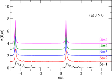
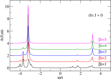
Figure 2: (color online) Spectral function $A(0,\omega)$ for different temperatures and FM (top) and AFM (bottom) coupling. Parameters are $|J|/t=0.5,\ J_{0}/t=2.5,\ h=0,\ \eta/t=0.04$.

IV.2 finite-T numerical results

We now discuss the results of the Monte Carlo simulations. In Fig. 2 we plot $k=0$ spectral functions for different values of $\beta$ for both FM and AFM couplings. In both cases the $\beta t=5.0$ results are in very good agreement with those at $T=0$, defining “low-temperatures” to mean $\beta t\geq 5$. As $\beta$ decreases ($T$ increases), the sharp peaks broaden considerably and new peaks appear. For FM coupling, the lowest energy state still lies at the bottom of the low-energy $T=0$ band. For AFM coupling, however, new states appear below the $T=0$ spectrum. This is expected since at finite-$T$ FM domains can form in the AFM background and the carrier lowers its energy when located in such domains. Of course, these energies are bounded from below by the lowest FM eigenenergy.

At first sight the appearance of these new peaks (in fact resonances, as discussed below) may seem to signal lack of convergence of the MC simulations, or finite-size issues related to a $M_{c}$ cutoff that is not big enough. However, the results are converged and do not change upon further $M_{c}$ increase; these features are real.

The appearance of similar features is a well documented phenomenon for the disordered binary alloys with which our problem has similarities, as discussed above. Studies of binary alloys have revealed that these peaks (which are truly discrete states, in that context) mark the appearance of bound states where the carrier is trapped by small clusters of like-atoms.Economou (2006); Dean (1972) As we show now, the resonances we observe have similar origin. For instance, in the FM case they are due to the charge carrier being trapped into spin-down domains formed into an otherwise spin-up background, or vice versa.

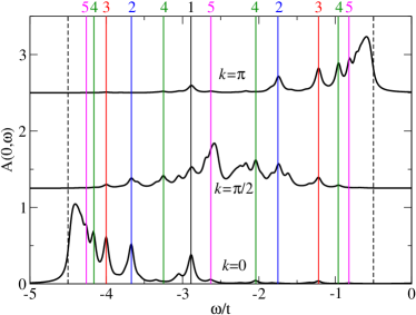
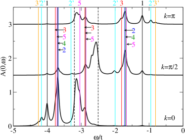
Figure 3: (color online) Spectral functions $A(k,\omega)$ for $\beta t=1$ and $k=0,\pi/2,\pi$, for FM (top) and AFM (bottom) coupling. Solid vertical lines mark the trapping energies of the carrier in small domains. The corresponding numbers show the length of the domain (see Table 1). The dashed vertical lines mark the band-edges of the $T=0$ low-energy band. Other parameters are $|J|/t=0.5,\ J_{0}/t=2.5,\ h=0,\ \eta/t=0.04$.

Color	Length	FM domain	AFM domain
black	1	$\dots\uparrow\uparrow\underline{\downarrow}\uparrow\uparrow\dots$	$\dots\uparrow\downarrow\underline{\downarrow}\downarrow\uparrow\dots$
blue	2	$\dots\uparrow\uparrow\underline{\downarrow\downarrow}\uparrow\uparrow\dots$	$\dots\uparrow\downarrow\underline{\downarrow\uparrow}\uparrow\downarrow\dots$
red	3	$\dots\uparrow\uparrow\underline{\downarrow\downarrow\downarrow}\uparrow\uparrow\dots$	$\dots\downarrow\uparrow\underline{\uparrow\downarrow\uparrow}\uparrow\downarrow\dots$
green	4	$\dots\uparrow\uparrow\underline{\downarrow\downarrow\downarrow\downarrow}\uparrow\uparrow\dots$	$\dots\downarrow\uparrow\underline{\uparrow\downarrow\uparrow\downarrow}\downarrow\uparrow\dots$
magenta	5	$\dots\uparrow\uparrow\underline{\downarrow\downarrow\downarrow\downarrow\downarrow}\uparrow\uparrow\dots$	$\dots\uparrow\downarrow\underline{\downarrow\uparrow\downarrow\uparrow\downarrow}\downarrow\uparrow\dots$
cyan	2’	-	$\dots\uparrow\downarrow\underline{\downarrow\downarrow}\downarrow\uparrow\dots$
yellow	3’	-	$\dots\uparrow\downarrow\underline{\downarrow\downarrow\downarrow}\downarrow\uparrow\dots$

Table 1: List of the shortest domains (underlined spins) that form in otherwise ordered backgrounds. The energies for trapping the carrier in these domains are shown in Fig. 3.

We calculated the eigenenergies for trapping the carrier inside several such short domains embedded in an otherwise ordered FM or AFM background. These values (various lines) are compared to the spectral weights obtained for $\beta t=1$ and $k=0,\pi/2,\pi$ in Fig. 3. The integers labelling the lines show the length of the corresponding domains, also see Table 1. The agreement between these trapping energies and the location of the resonances in $A(k,\omega)$ is very good. The weights of these resonances vary strongly with $k$ but their energies are nearly dispersionless. For AFM coupling, the trapping energies in different domains are sometimes very similar, suggesting that here trapping occurs at the boundaries of the domain, not inside its bulk; this explains the broader features at $\omega/t\approx-3.7,-2.9$ and $-1.7$.

Figure 4: $A(k,\omega)$ for different values of $k$ and FM coupling, at $J/t=0.5,\ J_{0}/t=2.5,\ \beta t=1.0,\ h=0,\ \eta/t=0.04$.

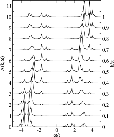
Figure 5: $A(k,\omega)$ for different values of $k$ and AFM coupling, at $J/t=-0.5,\ J_{0}/t=2.5,\ \beta t=1.0,\ h=0,\ \eta/t=0.04$.

To better understand the momentum dependence, complete sets of spectral weights are shown in Figs. 4 and 5 for FM and AFM coupling, respectively. For simplicity we do not mark the trapping energies of the carrier in the various domains, but we have checked that the agreement is as good as in Fig. 3 at all $k$.

For FM coupling, we see the two bands that have evolved from the $T=0$ peaks moving with increasing $k$ in a way that roughly mirrors the $T=0$ dispersions shown in Fig. 1(a). As $k$ increases, spectral weight is systematically shifted from the lower to the upper edge of each band. In addition we notice a small spectral weight transfer from the lower band to the upper band. This is in contrast to the FM $T=0$ solution, where both peaks have equal spectral weight. For AFM coupling, the $\pi$-periodicity of the $T=0$ dispersion is partially masked by the many additional resonances that appear on both sides of the $T=0$ peaks, and the significant transfer of spectral weight from the lower to the upper band. The latter is similar to the behavior observed for the $T=0$ solution. In both cases, the location of the various resonances does not change appreciably with $k$.

To understand the physical origin of these resonances, consider the analogy with the binary alloy model, which also shows such “peaky” structures in its total density of states (DOS), marking the bound states of the carrier inside small clusters of like-atoms.Economou (2006); Dean (1972) As is well known, in the presence of any amount of on-site disorder all eigenstates of a 1D chain become localized. To find the DOS one can formally calculate the disorder averaged Green’s function (which regains invariance to translations) but this quantity has no physical meaning. This is because in any real system there is a given disorder distribution, and if all eigenstates are localized then the carrier occupies forever the same small region of space and self-averaging does not occur. In other words, if the carrier is trapped in a cluster of atoms it will stay trapped indefinitely.

Each configuration of the binary alloy can be mapped into a spin configuration of the Ising chain, by replacing atoms A/B by spins up/down. Small clusters of like-atoms then map into magnetic domains, and there are trapped states of the carrier inside them, as already shown. However, unlike the fixed disorder configuration, the spin configuration changes continuously through thermal fluctuations. A trapped carrier therefore has a finite lifetime linked to the persistence of that domain: eventually the local spin configuration changes and the carrier is released to move along the chain. This is why here the “peaky” structures indicate actual finite life-time resonances for extended eigenstates of well-defined momentum, not infinitely-lived localized states like in the alloy model. This is a significant qualitative difference.

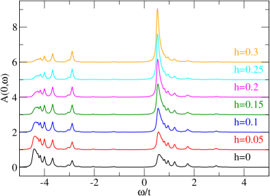
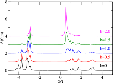
Figure 6: (color online) Spectral functions $A(0,\omega)$ for different values of $h$, for FM (top) and AFM (bottom) coupling. Other parameters are $|J|/t=0.5,\ J_{0}/t=2.5,\ \beta t=1.0,\ \eta/t=0.04$.

We conclude this section by considering the role of the external magnetic field $h$. Its effects on the $k=0$ spectral weight are shown in Fig. 6. For FM coupling we find that as $h$ increases, the initially large feature at the bottom of the lower band starts to disappear and most of its weight is moved to the bottom of the upper band. This is expected since the external field favors/disfavors the spin-up/down background responsible for this main feature (evolved from the $T=0$ peak) of the upper/lower band. Interesting, however, most of the resonances in the lower band remain almost unchanged. The reason is that while $\beta h\ll 1$, the energy cost for a small domain is very low so their appearance is very likely. If $\beta h\gg 1$ the Ising chain is forced into the $m>0$ ground state and only the higher $T=0$ peak survives (not shown).

For AFM coupling the effect of $h$ is more dramatic, as it forces the system into the $m>0$ FM ground-state if $\beta h$ becomes large enough. Indeed, for large $h$ most of the weight is moved into the upper FM peak and most of the resonances disappear, except for the one at $\omega/t\approx-2.9$ that is still quite large. Its energy is very close to that of the first FM cluster listed in Table 1, and indeed it seems plausible that this is due to a single flipped spin which entraps the carrier. This domain is disfavored by $h$, but actually lowers the exchange energy with its neighbors.

Note that we used different field strengths for the FM and AFM cases. In the latter case much higher fields are needed to produce long range correlations since there is a competition between the exchange energy of neighboring spins and the external field. A measure for this is the spin-spin correlation function $\langle\sigma_{-M_{c}}\sigma_{M_{c}}\rangle$, which for the parameters used in Fig. 6 equals 0.41 (FM, if $h/t=0.3$) and 0.64 (AFM, if $h/t=2.0$). A value of $\langle\sigma_{-M_{c}}\sigma_{M_{c}}\rangle=1$ means that the chain is completely ordered.

IV.3 Analytic approximation

We now use the insights gained from the Monte Carlo results to propose an analytic approximation for the GF at low and medium temperatures. We present the derivation only for the case of FM coupling when $h=0$; the other cases can be treated similarly.

The main idea is to only consider a limited number of spin configurations when performing the thermal average, to allow for its (quasi)analytic evaluation. Since our numerical results show the importance of small domains, the configurations we select are the two ordered configurations $|\text{FM},\sigma\rangle$ with all spins pointing up or down, $\sigma=\uparrow,\downarrow$ together with the one-domain configurations:

$$|n,n+l,\uparrow\rangle=4^{-(l+1)}\hat{\sigma}_{n}^{-}\cdot\hat{\sigma}_{n+1}^{-}\cdot\dots\hat{\sigma}_{n+l}^{-}|\text{FM},\uparrow\rangle$$ (20)

$$|n,n+l,\downarrow\rangle=4^{-(l+1)}\hat{\sigma}_{n}^{+}\cdot\hat{\sigma}_{n+1}^{+}\cdot\dots\hat{\sigma}_{n+l}^{+}|\text{FM},\downarrow\rangle,$$ (21)

where the domain starts at site $n$ and ends at $n+l$. The operator $\hat{\sigma}_{i}^{\pm}$ is the raising/lowering operator for the $i^{th}$ Ising spin. To preserve translational invariance we need to consider all possible locations of the domain within the Ising chain. All these one-domain states are weighed by the same Boltzmann factor $\mathrm{e}^{-4\beta J}$ (we take the energy of the fully ordered FM states as reference).

As discussed, a physically meaningful result has equal contributions from the spin-down and spin-up sectors. We now discuss the spin-up contribution, which we denote by $G_{\uparrow}(k,\omega)$. The spin-down contribution $G_{\downarrow}(k,\omega)$ is then obtained by simply letting $J_{0}\rightarrow-J_{0}$, and the GF is given by $G(k,\omega)=[G_{\uparrow}(k,\omega)+G_{\downarrow}(k,\omega)]/2$. By itself, the decomposition into an up-part and a down-part is not an approximation. The approximation stems from the fact that we are only considering the one-domain configurations when calculating $G_{\uparrow}(k,\omega),G_{\downarrow}(k,\omega)$.

By only considering domains up to a maximal length $L$ (for reasons discussed below), we thus approximate:

$$G_{\uparrow}(k,\omega)=\frac{1}{Z}\left[G_{\uparrow}^{\text{FM}}(k,\omega)+\mathrm{e}^{-4\beta J}\sum_{l=0}^{L}\mathcal{G}_{\uparrow}^{(l+1)}(k,\omega)+\dots\right]$$ (22)

where $Z=1+\mathrm{e}^{-4\beta|J|}L\cdot N+\dots$. The thermodynamic limit $N\rightarrow\infty$ will be taken at a later stage. The first contribution, from the ordered state, is

$$G_{\uparrow}^{\text{FM}}(k,\omega)=\langle\text{FM},\uparrow|c_{k}\hat{G}(\omega+\hat{H}_{\text{I}})c_{k}^{\dagger}|\text{FM},\uparrow\rangle$$

$$=\frac{1}{\omega-\varepsilon(k)-J_{0}+i\eta}.$$ (23)

To find the contributions

$$\mathcal{G}_{\uparrow}^{(l+1)}(k,\omega)=\sum_{n}\langle n,n+l,\uparrow|c_{k}\hat{G}(\omega+\hat{H}_{\text{I}})c_{k}^{\dagger}|n,n+l,\uparrow\rangle$$ (24)

from the states with a domain of length $l$, we have to work harder. Using Dyson’s identity once we obtain:

$$\mathcal{G}_{\uparrow}^{(l+1)}(k,\omega)=G_{\uparrow}^{\text{FM}}(k,\omega)\left[N-2J_{0}\sum_{m=0}^{l}f_{\uparrow,k}^{(l+1)}(m,\omega)\right],$$ (25)

where we defined the auxiliary GFs:

$$f_{\uparrow,k}^{(l+1)}(m,\omega) =\sum_{n}\frac{\mathrm{e}^{ikR_{n+m}}}{\sqrt{N}}$$

$$\langle n,n+l,\uparrow|c_{k}\hat{G}(\omega+\hat{H}_{\text{I}})c_{n+m}^{\dagger}|n,n+l,\uparrow\rangle.$$ (26)

Using Dyson’s equation again we find:

$$f_{\uparrow,k}^{(l+1)}(m,\omega)=G_{\uparrow}^{\text{FM}}(k,\omega)$$ (27)

$$-2J_{0}\sum_{m^{\prime}=0}^{l}g_{\uparrow}^{\text{FM}}(m^{\prime}-m,\omega) \mathrm{e}^{ik(R_{m}-R_{m}^{\prime})}f_{\uparrow,k}^{(l+1)}(m^{\prime},\omega),$$

where $g_{\uparrow}^{\text{FM}}(m^{\prime}-m,\omega)={1\over N}\sum_{q}\mathrm{e}^{iq(R_{m^{\prime}}-R_{m})}G_{\uparrow}^{\text{FM}}(q,\omega)$ are easy to find analytically. This is a linear system of $l+1$ equations that is solved to find all $f_{\uparrow,k}^{(l+1)}(m,\omega)$, which are then used in Eq. (25). Note that all $f_{\uparrow,k}^{(l+1)}(m,\omega)$ are proportional to $G_{\uparrow}^{\text{FM}}(k,\omega)$, since the latter quantity provides the inhomogeneous terms in this linear system.

When Eq. (25) is inserted in Eq. (22), if we group all terms proportional to $G_{\uparrow}^{\text{FM}}(k,\omega)$ we see that its factor $1/Z$ is cancelled. Higher order terms corresponding to states with two or more domains (not included in this calculation) should similarly cancel the factor $1/Z$ for the remaining terms in Eq. (22), or at least make the thermodynamic limit of the ratio meaningful. To ${\cal O}(e^{-4\beta J})$ order and for $N\rightarrow\infty$, we therefore find:

$$G_{\uparrow}(k,\omega) \approx\left[1-2J_{0}\mathrm{e}^{-4\beta J}\sum_{l=0}^{L}\sum_{m=0}^{l}f_{\uparrow,k}^{(l+1)}(m,\omega)\right]$$

$$G_{\uparrow}^{\text{FM}}(k,\omega).$$ (28)

Eq. (28) obeys the sum rule $\int_{-\infty}^{+\infty}\mathrm{d}\omega\,A(k,\omega)=1$ if the second term has no poles in the upper half of the complex plane. This is because the second term is proportional to $[G^{\text{FM}}_{\uparrow}(k,\omega)]^{2}$ and therefore falls of like $1/\omega^{2}$ as $|\omega|\rightarrow\infty$.

One may use Eq. (28) to extract a low-$T$ approximation for the self energy:

$$\Sigma_{\uparrow}(k,\omega)\approx-2J_{0}\mathrm{e}^{-4\beta J}\sum_{l=0}^{L}\sum_{m=0}^{l}\frac{f_{\uparrow,k}^{(l+1)}(m,\omega)}{G_{\uparrow}^{\text{FM}}(k,\omega)},$$ (29)

and define $G_{\uparrow}(k,\omega)\approx\left[[G_{\uparrow}^{\text{FM}}(k,\omega)]^{-1}-\Sigma_{\uparrow}(k,\omega)\right]^{-1}$ instead of $G_{\uparrow}(k,\omega)\approx G_{\uparrow}^{\text{FM}}(k,\omega)\left[1+\Sigma_{\uparrow}(k,\omega)G_{\uparrow}^{\text{FM}}(k,\omega)\right]$ of Eq. (28). At low enough temperatures both give the same results, but at higher temperatures the former approximation leads to spurious polesMöller and Berciu (2013) in the spectral weight so we use Eq. (28) in the following.

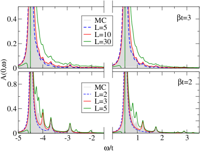
Figure 7: (color online) Comparison between the Monte Carlo (MC) results (shaded area) and the analytic approximation of Eq. (28) for domains with a maximal length of $L$, for FM coupling $J/t=0.5$, at $J_{0}/t=2.5,\ h=0,\eta/t=0.04,\ \ k=0$ and $\beta t=3$ (top) and $\beta t=2$ (bottom).

Results for FM and AFM coupling are shown in Figs. 7 and 8, respectively, for various lengths $L$ of the largest domain included, at two temperatures. For comparison, the Monte Carlo results are also shown (shaded regions). The quality of the approximation varies substantially with $L$. The top panel of Fig. 7 shows that for $\beta t=3$ and $L=5$, the weight of the resonances is underestimated and not all of them are reproduced by the approximation. For $L=10$ the agreement between the approximation and the exact results is very good, but it worsens again for $L=30$. Not only does the latter overestimate the weight of the resonances, but it also predicts negative spectral weight just below the bands. While this negative weight is needed to satisfy the sum rule, its presence is unphysical and signals a failure of the approximation. The same trends are observed for $\beta t=2$ in the bottom panel of Fig. 7. Here the best agreement is obtained at $L=3$, although resonances associated with longer domains are missing. They appear for $L=5$, however so does the unphysical behavior. For even lower values of $\beta$ the approximation fails completely to capture the correct weight of the resonances, although, as shown in Fig. 3, their locations are due to carrier trapping in domain walls.

The AFM approximation yields very similar results. The top panel of Fig. 8 shows that again for $\beta t=3$ excellent agreement with the exact solution is reached for $L=10$, while for larger values of $L$ the weight of the resonances is overestimated and unphysical behavior occurs if $L=30$. For $\beta t=2$ the agreement with the exact solution is best for $L=4$ and unphysical behavior already occurs at $L=6$. Again the approximation fails badly to capture the proper weight of various features, for smaller values of $\beta$ (higher $T$).

Naively, one may expect the approximation to improve when $L$ is increased since this means that a larger fraction of the possible configurations is considered. However, there are two factors which determine how a domain contributes to the thermal average. One is the additional energy cost of a domain, which is accounted for by the Boltzmann factor and in 1D does not depend on the domain’s length. The other is the increase in entropy with increasing number of domains. As the temperature increases, minimization of the free energy $F=U-TS$ is increasingly driven by entropy maximization, resulting in more domains and thus shorter correlations. The order of magnitude for the maximal domain size should be given by the spin-spin correlation length $\xi$ (defined in the Appendix). Indeed, we obtain $\xi\approx 4$ and $\xi\approx 10$ for $\beta t=2$ and $\beta t=3$, respectively. This compares well with the values of $L$ where the approximation performs well, see Figs. 7 and 8.

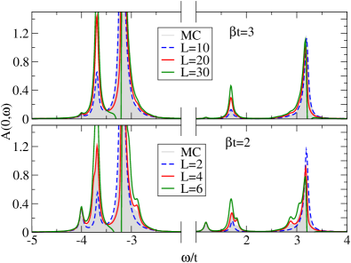
Figure 8: (color online) Same as in Fig. 7 but for AFM coupling $J/t=-0.5$.

Another way to see why the approximation with $L\rightarrow\infty$ is bound to become wrong is to realize that all domain walls whose length is longer than the distance explored by the carrier within its lifetime are actually indistinguishable from the “other” ordered FM configuration, from the point of view of the carrier. In other words, all these configurations essentially contribute a $G_{\downarrow}^{\text{FM}}(k,\omega)$, and their inclusion gives the wrong weighting to the $|\text{FM},\downarrow\rangle$ contribution. Similarly, configurations with two long domain walls placed relatively close together will have states where the carrier is trapped in the short region between the domains, indistinguishable from having a short domain formed in the “other” ordered FM configuration. Adding many such contributions will affect the weights of these one-domain contributions, etc. These arguments suggest that a better approximation is:

$$G_{\uparrow}(k,\omega)=\left[1-\sum_{l=0}^{N/2}w_{l}(\beta)\sum_{m=0}^{l}f_{\uparrow,k}^{(l+1)}(m,\omega)\right]G_{\uparrow}^{\text{FM}}(k,\omega)$$ (30)

with $\left.G_{\downarrow}(k,\omega)=G_{\uparrow}(k,\omega)\right|_{J_{0}\rightarrow-J_{0}}$, where $w_{l}(\beta)$ are adjusted to capture accurately the weight of resonances due to trapping into short domains. For low and medium temperatures we showed that $w_{l}(\beta)=2J_{0}e^{-4\beta J}$ if $l\leq\xi$, and zero otherwise, gives very decent predictions. Clearly this cannot work at high temperatures of order $\beta t=1$ where $\xi\rightarrow 0$. So far we have been unable to think of a reasonable form of $w_{l}(\beta)$ in this regime, but the comparisons displayed in Fig. 3 suggest that it should exist.

V Conclusions

To summarize, we obtained numerically exact spectral functions for a simplified model of a carrier injected into a 1D Ising chain at finite-$T$. The results highlight the importance of small domains that can trap the carrier, which were shown to be responsible for the resonances that appear as $T$ increases. A simple analytic approximation based on these ideas was found to perform well at low and medium temperatures. With further insights, it may be possible to generalize it to high temperatures, as well. Interestingly, chains with both FM and AFM coupling can be understood in similar terms, although generically one expects quite different phenomenology for a carrier injected into a FM vs AFM background.

As highlighted throughout, there are parallels between this problem and that of a carrier moving in a random binary alloy, where the importance of small clusters of like-atoms, equivalent to the small domains of our model, is well documented.Dean (1972); Economou (2006); Alben et al. (1975) There are, however, also major differences: finite $J$ maps into correlations between the atoms of the alloy (usually these are ignored). The thermal average is also very different, both qualitatively and quantitatively, from a disorder average. It is therefore not a priori clear how much of the considerable amount of work devoted to finding analytic approximations for binary alloys can be used for the magnetic problem.

In terms of generalizations, one direction is to see how far these insights carry over to higher dimensions, where long-range magnetic order survives at finite $T$. For binary alloys it is known that the fine-structure of the spectral function is most dominant in 1D.Economou (2006) For our model, the energy cost scales with the domain size in 2D and 3D, unlike in 1D and unlike for a binary alloy. This may well lead to a behavior that is different from that of the binary alloys and could cause the fine-structure associated with very small domains to remain present in higher dimensions, at least at low temperatures.

Another interesting direction is to allow for Heisenberg coupling between the carrier and the local moments (still with Ising coupling between the latter). In this case spin-flip processes become possible. The carrier can move small domains around (in fact, the spin-polaronShastry and Mattis (1981); Berciu and Sawatzky (2009) can be thought of as a mobile bound state between the carrier and a one-site domain), or split longer domains into several smaller ones, etc. Understanding the consequences of such processes and their effect on the finite-$T$ spectral function would be very useful. Even more complicated is the case with Heisenberg coupling between the lattice spins. Clearly there is a lot of work, both numerical and analytical, to be done before these problems are solved.

Our results underline the importance of the local environment for the behavior of a charge carrier in a magnetic background, at least for this model and in low dimension. Incorporating these effects is difficult since mean-field approximations cannot capture them. The only real alternative is to obtain an understanding of which states of the environment contribute most to the temperature average, and to propose approximations based on taking the average over this limited set of states. Our work presents the first step in this process.

*

Appendix A Exact solution of the undoped Ising chain

Here we review the exact solution of the undoped Ising chain. All quantities of interest to us are obtained from the partition function:

$$Z=\sum_{\{\sigma\}}\mathrm{e}^{-\beta E_{I}(\{\sigma\})},$$ (31)

where the sum is over all configurations of lattice spins. The sum can be rewritten as:

$$Z=\operatorname{Tr}(\mathcal{T}^{N})=\lambda_{+}^{N}+\lambda_{-}^{N},$$

where the transfer matrix is $\mathcal{T}_{\sigma,\sigma^{\prime}}=\mathrm{e}^{\beta(J\sigma\sigma^{\prime}+\frac{h}{2}(\sigma+\sigma^{\prime}))}$, and its eigenvalues are:

$$\lambda_{\pm}=\mathrm{e}^{\beta J}\left[\cosh(\beta h)\pm\sqrt{\sinh^{2}(\beta h)+\mathrm{e}^{-4\beta J}}\right].$$ (32)

The bulk value of the magnetization $m={1\over N}\sum_{i}\langle\hat{\sigma}_{i}\rangle_{T}$ is:

$$m=\lim_{N\rightarrow\infty}{1\over N\beta}\frac{\partial\ln Z}{\partial h}=\frac{\sinh(\beta h)}{\sqrt{\sinh^{2}(\beta h)+\mathrm{e}^{-4\beta J}}}.$$ (33)

The correlation between spins is given by

$$\langle\sigma_{n}\sigma_{m}\rangle_{T}=\frac{\sinh^{2}(\beta h)+\mathrm{e}^{-4\beta J}\mathrm{e}^{-|m-n|/\xi}}{\sinh^{2}(\beta h)+\mathrm{e}^{-4\beta J}},$$ (34)

where the correlation length is $\xi=1/\log(\lambda_{-}/\lambda_{+})$. (For AFM coupling one needs to factor out $(-1)^{|m-n|}$ to ensure the real-valuedness of $\xi$).