Dipolar ordering and domains in crystals of Mn₁₂ Ac molecular magnets

Abstract

Dipolar coupling in crystals of the Mn₁₂Ac molecular magnet elongated along the anisotropy axis favors ferromagnetic ordering below the mean-field Curie temperature 0.71 K. With the help of Monte Carlo on crystals of up to one million Mn₁₂ molecules, it is shown that ordering occurs at 0.36 K. The resulting state is split into ferromagnetic domains with domain walls preferring the diagonal orientation. Domain walls are pinned by the lattice at low temperatures. Making the crystal shorter makes domains finer and smoothens out the singularity at the transition, decreasing susceptibility in the domain state. Hysteresis loops look ferromagnetic for prolate crystals and antiferromagnetic for oblate crystals.

I Introduction

Magnetic ordering in crystals of molecular magnets, caused by the dipole-dipole interaction (DDI), is especially interesting because of its close relation to the spectacular phenomenon of spin tunneling under the barrier created by the strong uniaxial anisotropy frisartejzio96prl (for a recent review, see Ref. MM14springer ). The most famous of molecular magnets is Mn₁₂Ac, each molecule of which behaves as a giant spin $S=10$ that can point in two directions along the easy axis. Mn₁₂Ac crystallizes into a body-centered tetragonal lattice with the periods $a=b=17.319$ Å and $c=12.388$ Å, $c$ being the direction of the magnetic easy axis $z$.

There is no exchange interaction between the molecules, the strongest interaction being the DDI. In prolate crystals the DDI is creating the dipolar field $B_{z}^{(D)}=0.0526$ T (Ref. garchu08prb ) that was also measured in experiment mchughetal09prb . Such strong dipolar bias affects the resonance condition for spin tunneling and makes it collective. In addition to experimentally observed magnetic deflagration suzetal05prl ; garchu07prb , fast dipolar-controlled fronts of tunneling were proposed gar13prb .

The possibility of dipolar ordering in different molecular magnets was considered in Ref. feralo00prb , where Monte Carlo simulations on small systems were done. Energies of different types of dipolar ordering in another molecular magnet Fe₈ were computed in Ref. marchuaha01epl . Neutron-diffraction experiments on Mn₁₂Ac in transverse magnetic field luietal05prl suggested ferromagnetic ordering below about 1 K. Dipolar ordering was observed by magnetic measurements in Fe₁₇ compound with $S=35/2$ evaetal06prl and in Mn₆ compound with $S=12$ moretal06prb , both materials having a small anisotropy.

The mean-field-based theory of dipolar ordering, domain-wall structure and domain-wall motion in Mn₁₂Ac was developed in Ref. garchu08prb . Measurements of the magnetic susceptibility of Mn₁₂Ac on the high-temperature side suggest its divergence at a finite temperature, indicative of a phase transition milkensaryes10prb ; bowenetal10prb . Theoretically, for elongated crystals with the aspect ratio exceeding 6 (Ref. gar10prbrc ) uniform ferromagnetic ordering has lower energy than ordering with alternating ferromagnetic columns or planes garchu08prb . However, in Ref. gar10prbrc by solving the space-resolved Curie-Weiss equation it was shown that ordering occurs into the ferromagnetic state with domains rather than into the uniform ferromagnetic state. In Ref. burzurietal11prl magnetic ordering in Fe₈ was observed at $T=0.34$ K by magnetic measurements.

The purpose of the work presented in this paper was to elicudate dipolar-driven magnetic ordering in Mn₁₂Ac by large-scale Monte Carlo simulations. Of a particular interest is dependence of the domain structure on the aspect ratio of the crystals. Simulation of a ferromagnetic state with domains requires a large crystal size, thus crystals containing up to a million of magnetic molecules were used in computations. For so large system sizes the long-range character of the DDI creates a computational problem. Thus a modification of the Monte Carlo procedure regarding updating the dipolar field was done that allowed a considerable speed-up.

The main part of this article is organized as follows. The model is introduced in Sec. II, where a short survey of the previously obtained results is done. Sec. III is devoted to elucidation the role of coulumns of spins along the $c$ axis, the main boulding block of the order in Mn₁₂Ac. Here the optimal configuration of domain walls is found and estimations for the domain structure are done. In Sec. IV the numerical method, especially concerning the dipolar-field update, is described in detail. Sec. V presents numerical results and compares them with predictions of Sec. III.

II The model

The model of the Mn₁₂Ac crystal includes pseudospin variables $\sigma_{i}=\pm 1$ for molecules at each lattice site $i$ of a boby-centered tetragonal lattice. The magnetic moment of a molecule is $Sg\mu_{B}$ with $g=2.$ The dipole-dipole interaction in molecular magnets is due to the longitudinal components of the spins only and can be written in the form

$$\mathcal{H}\equiv-\frac{E_{D}}{2}\sum_{i,j}\phi_{ij}\sigma_{iz}\sigma_{jz},$$ (1)

where $E_{D}=\left(Sg\mu_{B}\right)^{2}/v_{0}$ is the dipolar energy, $E_{D}/k_{B}=0.0671$ K for Mn₁₂Ac, $v_{0}=abc$ is the unit-cell volume and

$$\phi_{ij}=v_{0}\frac{3\left(\mathbf{e}_{z}\cdot\mathbf{n}_{ij}\right)^{2}-1}{r_{ij}^{3}},\qquad\mathbf{n}_{ij}\equiv\frac{\mathbf{r}_{ij}}{r_{ij}}.$$ (2)

The position vector on one of the sublattices can be written as

$$\mathbf{r}_{i}=i_{a}a\mathbf{e}_{a}+i_{b}b\mathbf{e}_{b}+i_{c}c\mathbf{e}_{c},\qquad i_{a},i_{b},i_{c}=0,\pm 1,\pm 2,\ldots$$ (3)

and that on the other sublattice is given by the same expression with the indices $i_{a},i_{b},i_{c}$ shifted by 1/2. Thus the reduced DDI can be put into the form $\phi_{ij}=\phi\left(i_{a}-j_{a},i_{b}-j_{b},i_{c}-j_{c}\right)$ with

$$\phi\left(n_{a},n_{b},n_{c}\right)=\eta\frac{2\eta^{2}n_{c}^{2}-n_{a}^{2}-n_{b}^{2}}{\left(n_{a}^{2}+n_{b}^{2}+\eta^{2}n_{c}^{2}\right)^{5/2}},\qquad\eta\equiv\frac{c}{a},$$ (4)

where $\eta=0.7153$ for Mn₁₂Ac.

The dipolar field on magnetic molecule $i$ is the sum over positions of all other molecules $j$

$$B_{i,z}^{(D)}=\frac{Sg\mu_{B}}{v_{0}}D_{i,zz},\qquad D_{i,zz}\equiv\sum_{j}\phi_{ij}\sigma_{jz},$$ (5)

where $D_{zz}$ is the reduced dipolar field. Inside a uniformly magnetized ellipsoid with the symmetry axis $z$, the dipolar field is uniform, so that one has $D_{zz}=\bar{D}_{zz}\sigma_{z}.$ Here

$$\bar{D}_{zz}=\bar{D}_{zz}^{(\mathrm{sph})}+4\pi\nu\left(1/3-n^{(z)}\right),$$ (6)

$\nu$ is the number of magnetic molecules per unit cell ($\nu=2$ for Mn₁₂ Ac) and $n^{(z)}=0,$ $1/3,$ and 1 for a cylinder, sphere, and disc, respectively. The reduced dipolar field in a sphere $\bar{D}_{zz}^{(\mathrm{sph})}$ depends on the lattice structure. For Mn₁₂Ac direct lattice summation yields $\bar{D}_{zz}^{(\mathrm{sph})}=2.155$ that results in $\bar{D}_{zz}^{(\mathrm{cyl})}=10.53$ for a cylinder garchu08prb . Then Eq. (5) yields the dipolar field $B_{z}^{(D)}\simeq 52.6$ mT in an elongated sample that was also obtained experimentally mchughetal09prb .

The ground-state energy in the above uniform state is given by

$$E_{0}=-(1/2)\bar{D}_{zz}E_{D},\qquad E_{D}\equiv\left(Sg\mu_{B}\right)^{2}/v_{0}.$$ (7)

The mean-field Curie temperature is given by garchu08prb

$$T_{C}=E_{D}\bar{D}_{zz}/k_{B}$$ (8)

that yields $T_{C}=0.707$ K.

States with ferromagnetically ordered planes alternating in the $a$ or $b$ directions in each sublattice of Mn₁₂ Ac have $\bar{D}_{zz}=9.480,$ independently of the sample shape garchu08prb . The state with alternating chains in each sublattice, directed along the $c$ direction has a very close value $\bar{D}_{zz}=9.475.$ For the two-sublattice antiferromagnetic ordering one obtains $\bar{D}_{zz}=8.102.$ Thus, in a strongly prolate ellipsoid of Mn₁₂ Ac ferromagnetic ordering is preferred. Below it will become clear that for box-shape crystals the results do not depend on the aspect ratio and the lowest-energy state is ferromagnetic with domains.

III Columns and domains

One can calculate the reduced dipolar field produced by an infinitely long column of ordered spins on one of its own sites. One obtains $D_{zz}=\bar{D}_{zz}\sigma_{z}$, where

$$\bar{D}_{zz}(0,0)=2\sum_{n=1}^{\infty}\phi\left(0,0,n\right)=\frac{4}{\eta^{2}}\sum_{n=1}^{\infty}\frac{1}{n^{3}}=\frac{4\zeta(3)}{\eta^{2}}$$ (9)

that for Mn₁₂Ac yields $\bar{D}_{zz}(0,0)=9.39742.$ This field is much larger than the field produced by such a column at any site that does not belong to it (see below). For this reason columns aligned along the $c$ axis are very stable and can be considered as a building block for magnetic ordering in Mn₁₂Ac.

Within the continuous approximation, the dipolar field produced by an infinite column of ordered spins disappears outside the column. In fact, however, some dipolar field due to the discreteness of the lattice remains, $D_{zz}<0$ at the sites of the same sublattice and $D_{zz}>0$ at the sites of the other sublattice [Eq. (3) of Ref. feralo00prb ]. This field decreases extremely fast with the distance from the column, so that it is sufficient to take into account only the interaction with nearest neighbors. With distances specified by $n_{\rho}$ and $n_{c}$ for Mn₁₂Ac one has

$$\bar{D}_{zz}\left(\frac{1}{\sqrt{2}},\frac{1}{\sqrt{2}}\right) = 0.303949$$ (10)

$$\bar{D}_{zz}\left(1,0\right) = -0.0197309$$ (11)

for the nearest neighbors in the other sublattice and the nearest neighbors in the same sublattice, respectively. The first line above suggests ferromagnetic ordering of neighboring colums and thus ferromagnetic ordering of the whole crystal. The total dipolar field at any site in the depth of the crystal is the sum of the field produced by the same column and by a few neighboring columns. For ferromagnetic ordering one finds

$$\bar{D}_{zz}^{(f\mathrm{erro})} \cong \bar{D}_{zz}(0,0)+4\bar{D}_{zz}\left(\frac{1}{\sqrt{2}},\frac{1}{\sqrt{2}}\right)+4\bar{D}_{zz}\left(1,0\right)$$ (12)

$$= 10.5343$$

that coincides with the value 10.53 previously found by a direct summation of dipolar field contributions garchu08prb . In the case of alternating ferromagnetic columns within each sublattice one obtains

$$\bar{D}_{zz}^{(110)}\cong\bar{D}_{zz}(0,0)-4\bar{D}_{zz}\left(1,0\right)=9.47634$$ (13)

that is very close to the value 9.475 found directly garchu08prb .

Let us consider now the effect of the surface. One can calculate the reduced dipolar field produced by a semi-infinite ordered column of spins at a site at a distance $\rho=an_{\rho}\equiv a\sqrt{n_{a}^{2}+n_{b}^{2}}$ away from the column and the vertical distance $z=cn_{c}$ from the end of the column (the surface of the crystal). It is given by

$$\bar{D}_{zz}(\rho,z)=\eta\sum_{n=-n_{c}}^{\infty}\frac{2\eta^{2}n^{2}-n_{\rho}^{2}}{\left(n_{\rho}^{2}+\eta^{2}n^{2}\right)^{5/2}}.$$ (14)

For $\rho\gg a$, i.e., $n_{\rho}\gg 1,$ one can replace summation by integration and obtain

$$\bar{D}_{zz}(\rho,z)=a^{2}\int_{-z}^{\infty}dz^{\prime}\frac{2z^{\prime 2}-\rho^{2}}{\left(\rho^{2}+z^{\prime 2}\right)^{5/2}}=-\frac{a^{2}z}{\left(\rho^{2}+z{}^{2}\right)^{3/2}}.$$ (15)

One can see that as the observation point moves inside the crystal, $z\rightarrow\infty,$ the dipolar field disappears. Physically, the magnetic field produced by a continuous semi-infinite row of magnetic dipoles only exits at the end of the row and has the same form as the field produced by a magnetic charge. Writing the result in the form

$$D_{zz}(\rho,z)=-\frac{a^{2}}{\rho^{2}+z^{2}}\frac{z}{\sqrt{\rho^{2}+z^{2}}}$$ (16)

one can see that the first fraction is the strength of the reduced magnetic field $\mathbf{B}^{(D)}$of a point magnetic charge while the second fraction is the projection cosine of the vector $\mathbf{B}^{(D)}$ upon the axis $c$.

The reduced interaction energy of two semi-infinite ordered columns at the distance $\rho\gg a$ from each other is given by the integral

$$e(\rho) = -\int_{0}^{\infty}\frac{dz}{c}\bar{D}_{zz}(\rho,z)$$ (17)

$$= \frac{a^{2}}{c}\int_{0}^{\infty}dz\frac{z}{\left(\rho^{2}+z{}^{2}\right)^{3/2}}=\frac{a^{2}}{c\rho}.$$

The interaction energy in real units $E\left(\rho\right)=E_{D}e(\rho)$ is given by

$$E\left(\rho\right)=\frac{q_{m}^{2}}{\rho},\qquad q_{m}=\frac{Sg\mu_{B}}{c}.$$ (18)

This means that two semi-infinite columns interact like two point changes $q_{m}$ at the ends of the columns.

Considering a slab of dimensions $L_{a}$, $L_{b}$, $L_{c}$ and using the density of the columns $1/(ab)=1/a^{2}$, the total energy associated with the ferromagnetically ordered surface can be estimated as

$$E_{\mathrm{surf}}^{(\mathrm{ferro)}} \sim \frac{E_{D}}{\left(a^{2}\right)^{2}}\intop\intop dxdydx^{\prime}dy^{\prime}e(\rho)$$ (19)

$$= \frac{E_{D}}{a^{3}}\intop\intop\frac{dxdydx^{\prime}dy^{\prime}}{\rho}\sim E_{D}\frac{L_{\bot}^{3}}{a^{3}},$$

where $L_{\bot}\sim L_{a}\sim L_{b}$. This energy is positive that makes uniform ferromagnetic ordering of columns unfavorable and causes its splitting into domains. From Fig. 1 one can see that diagonal domain walls (b) have the energy per unit area by the factor $\sqrt{2}$ lower than domain walls along crystallographic planes (a). The domain-wall energy is mainly due to the intersublattice interaction, Eq. (10), and is equal to

$$\frac{1}{2}E_{D}\bar{D}_{zz}\left(\frac{1}{\sqrt{2}},\frac{1}{\sqrt{2}}\right)\frac{2}{c\left(a/\sqrt{2}\right)}=\sqrt{2}\times 0.304\frac{E_{D}}{ac}$$ (20)

per unit area.

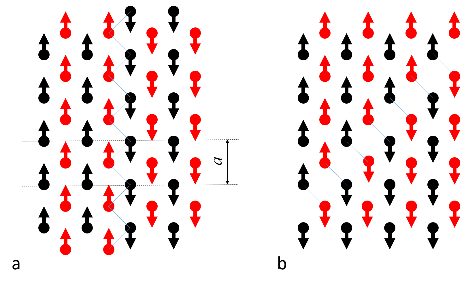
Figure 1: Crystal-plane (a) vs diagonal (b) domain walls. The latter have the energy per unit area by the factor $\sqrt{2}$ lower.

To estimate the domain size, one can assume that the crystal is split into a checkered pattern of up- and down-domains of the size $d$, so that there are $m=L_{\bot}/d$ domains in each transverse direction. The surface energy is due to the self-interaction within the islands of size $d^{2}$ and between the islands. Modification of Eq. (19) yields the estimation

$$E_{\mathrm{surf}}^{(\mathrm{domains)}}\sim m^{2}E_{D}\frac{d^{3}}{a^{3}}=E_{D}\frac{L_{\bot}^{2}d}{a^{3}}$$ (21)

that is smaller than Eq. (19). These domains create $\sim m$ domain walls having the energy

$$E_{\mathrm{vol}}^{(\mathrm{DWs)}}\sim mE_{D}\frac{L_{\bot}L_{c}}{ac}\sim E_{D}\frac{L_{\bot}^{2}L_{c}}{acd},$$ (22)

where factors of order 1 have been discarded. Minimizing the total excessive energy due to the surface charges and domain walls per magnetic molecule

$$\delta E=\left(E_{\mathrm{surf}}^{(\mathrm{domains)}}+E_{\mathrm{vol}}^{(\mathrm{DWs)}}\right)\frac{a^{2}c}{L_{\bot}^{2}L_{c}}=E_{D}\left(\frac{d}{L_{c}}+\frac{a}{d}\right)$$ (23)

with respect to $d$, one obtains

$$d\sim\sqrt{aL_{c}},\qquad\delta E\sim E_{D}\sqrt{\frac{a}{L_{c}}}.$$ (24)

As for ordinary ferromagnets, the period of the domain structure $d$ does not depend on the transverse size of the crystal and increases with crystal length. Independence of the transverse size means independence of the aspect ratio for the box-shape crystals, in contrast to the crystals of the ellipsoidal shape (see the end of Sec. II). This finding will be checked numerically below.

Let us now estimate the magnetic susceptibility in the domain state assuming that applied magnetic field slightly shifts domain walls making the sizes of positive and negative domains different: $d\Rightarrow d_{\pm}=d\pm\delta d$. This changes spin polarization per molecule as

$$\left\langle\sigma_{z}\right\rangle=\frac{d_{+}^{2}-d_{-}^{2}}{d_{+}^{2}+d_{-}^{2}}\cong\frac{2\delta d}{d}.$$ (25)

The corresponding Zeeman energy is $-E_{D}\left\langle\sigma_{z}\right\rangle\tilde{B},$ where the reduced magnetic field $\tilde{B}$ is defined by $B=\left(Sg\mu_{B}/v_{0}\right)\tilde{B}.$ While the energy of domain walls does not change, the changed surface energy due to the spin polarization $\left\langle\sigma_{z}\right\rangle$, averaged over the domain structure, can be estimated by adding the factor $\left\langle\sigma_{z}\right\rangle^{2}$ to Eq. (19) that yields the additional energy

$$E_{\mathrm{surf}}^{(B)}\sim E_{D}\frac{L_{\bot}^{3}}{a^{3}}\left\langle\sigma_{z}\right\rangle^{2}\sim E_{D}\frac{L_{\bot}^{3}}{a^{3}}\frac{(\delta d)^{2}}{d^{2}},$$ (26)

c.f. Eq. (21). Thus the total energy per spin becomes

$$\delta E=E_{D}\left(\frac{d}{L_{c}}+\frac{L_{\bot}}{L_{c}}\frac{(\delta d)^{2}}{d^{2}}+\frac{a}{d}-\frac{\delta d}{d}\tilde{B}\right).$$ (27)

Minimizing this energy with respect to $\delta d$, one obtains $\delta d\sim\left(L_{c}/L_{\bot}\right)d\tilde{B}$. The corresponding reduced susceptibility per magnetic molecule becomes

$$\tilde{\chi}=\frac{\left\langle\sigma_{z}\right\rangle}{\tilde{B}}\sim\frac{\delta d}{d\tilde{B}}\sim\frac{L_{c}}{L_{\bot}},$$ (28)

the aspect ratio. For long crystals domains are strongly coupled to the magnetic field because of their length, thus the susceptibility can be very large. Finally, the saturation field can be estimated as

$$\tilde{B}_{s}\sim\frac{1}{\tilde{\chi}}\sim\frac{L_{\bot}}{L_{c}},$$ (29)

whereas in real units $B_{s}=\left(Sg\mu_{B}/v_{0}\right)\tilde{B}_{s}$.

IV Numerical method

Equilibrium properties of the molecular magnet Mn₁₂Ac were studied by the Metropolis Monte Carlo method making successive trial spin flips $\sigma_{iz}\rightleftharpoons-\sigma_{iz}$ at lattice sites $i$ and computing the ensuing energy change $\Delta E=-E_{D}D_{i,zz}\Delta\sigma_{iz}$. In the case $\Delta E<0$ the trial is accepted, while for $\Delta E>0$ the trial is accepted with the probability $\exp(-\Delta E/T)$. The trials themselves were done with the probability of 1/2 only that ensures a true stochastic behavior. If all trials are done, at high temperatures nearly 100% acceptance rate results in a nearly deterministic process leading to the state of the highest energy.

Early papers using Monte Carlo sumulations of small-size molecular magnets, e.g., Ref. feralo00prb , do not report the details of the procedure. For crystals of large size, however, the long-range dipolar interaction makes a straightforward application of the Monte Carlo procedure very slow, so that it has to be optimized.

First, the dipolar field in the crystal has to be computed by a procedure based on the fast Fourier transform (FFT) that takes the time nearly linear in the system size (the number of magnetic molecules $N$), in contrast to the direct summation in Eq. (5) that takes the time growing as $N^{2}$. Wolfram Mathematica that was used for computations here, allows to obtain dipolar fields at each site $i$ by the $\mathsf{ListConvolve}$ command making summation in Eq. (5) by a procedure internally implementing the FFT.

Second, even using the FFT takes a time $\sim N^{2}$ for a full system update, if the dipolar fields are recalculated before or after each trial. To reduce this time, the following approach was taken. Both spin values $\sigma_{iz}$ and the dipolar fields $D_{i,zz}$ are being fed into the Monte Carlo routine. In the case of a rejected trial, dipolar fields are not recalculated. In the case of accepted trial, only the dipolar fields on the neighboring sites were recalculated, here on up to the 5 neighboring sites along the $c$-direction and up to 2 neighboring sites in the perpendicular directions. This procedure is especially well justified at high temperatures, where spins are disordered and there is no long-range contribution to the dipolar field, whereas the short-range contribution decreases fast enough as $1/r^{3}$. At lower temperatures, the acceptance rate decreases and the change of the long-range field is small again. In any case, recalculating the short-range part of the dipolar field captures the main part of the effect and does not take much time so that the full system update takes a time $\sim N$. After the full system update of spins, one can make the global update of the dipolar field using the FFT-based $\mathsf{ListConvolve}$ command that again takes a time $\sim N$.

Measurements of the spent computer time showed that global updating of the dipolar fields, even with the FFT, takes much longer than the Monte Carlo updating of spins with recomputing the short-range fields. This allows a firther speed-up at low temperatures where acceptance rate of spin flips is low and the change of dipolar fields in one system update is small. One can make the costy global dipolar-field update only after a certain percentage of spins flipped during a number of full spin updates. Tests have shown that for large-size systems this maximal fraction of flipped spins is about 2%. Increasing this fraction to 3% and more leads to breaking columns of spins at the ends of the crystal at low temperatures that is an artifact of the approximation made. Indeed, at low temperatures, as the result of ordering, the long-range dipolar field becomes more important and less tolerant to approximations.

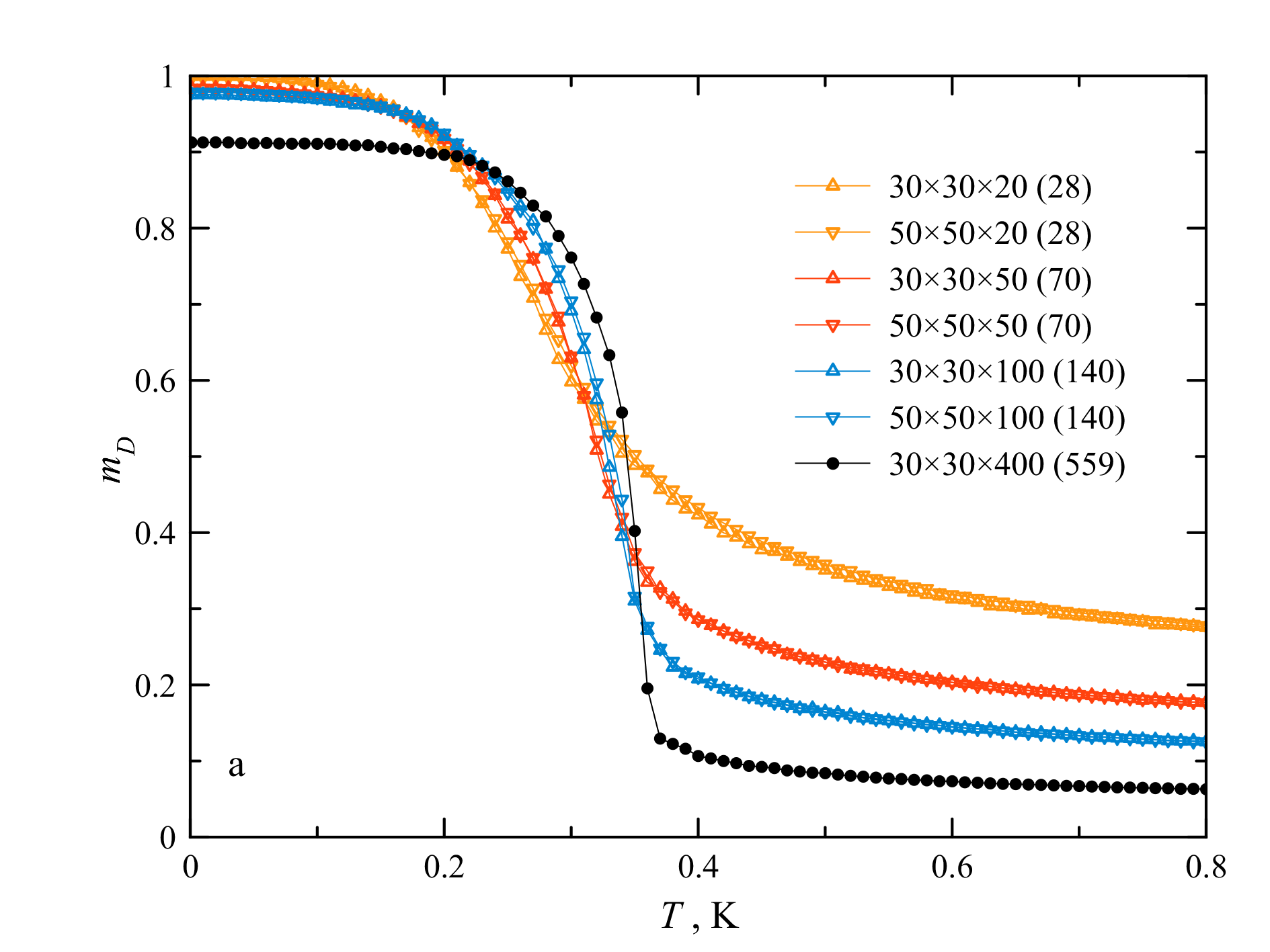
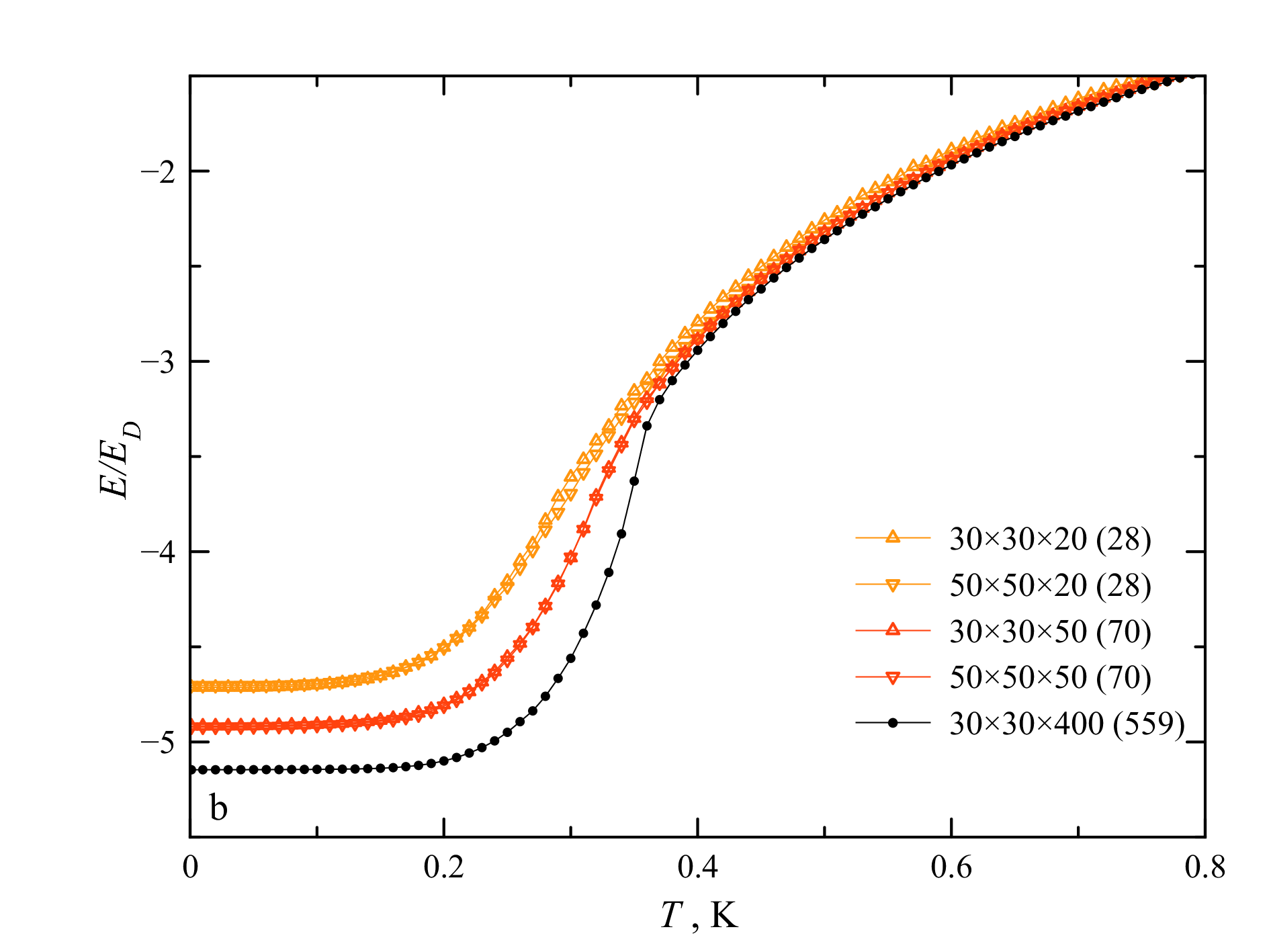
Figure 2: Temperature dependence of (a): domain order parameter $m_{D}$ and (b): reduced energy of box-shape crystals of Mn₁₂Ac. The shapes are labeled by $L_{a}\times L_{b}\times L_{c}(N_{c})$, where the linear sizes $L$ are in the units of $a$ and $N_{c}=L_{c}/\eta$. The number of magnetic molecules in the crystal is $2\times L_{a}\times L_{b}\times N_{c}$.

The stopping/measuring strategy used in the applied Monte Carlo procedure is the following. A block of Monte Carlo spin updates of the size NMC is defined, in most cases $\mathrm{NMC=100}$. This is the minimal number of Monte Carlo updates for each temperature or bias magnetic field. Inside this block of updates, the energy of the system was monitored and its mean value and dispersion were computed. The energy change over NMC updates was estimated as the double difference of the mean energy values over the first and second halfs of the NMC interval. When the energy change became less than a fraction of the energy dispersion, here 0.2, it was concluded that the system reached equilibrium, the procedure was stopped and the averages of physical quantities over the block of last NMC updates were computed. Above $T_{C}$ equilibration was very fast, so that the total number of updates was only slightly higher than NMC. Near $T_{C}$ critical slowing down was observed, and the total number of updates needed to reach equilibrium increased by a factor about three. Such quantities as the energy and magnetization are self-averaging with increasing the size of the system, so that for the sizes of about one million magnetic molecules $\mathrm{NMC=100}$ is sufficient to obtain good smooth data.

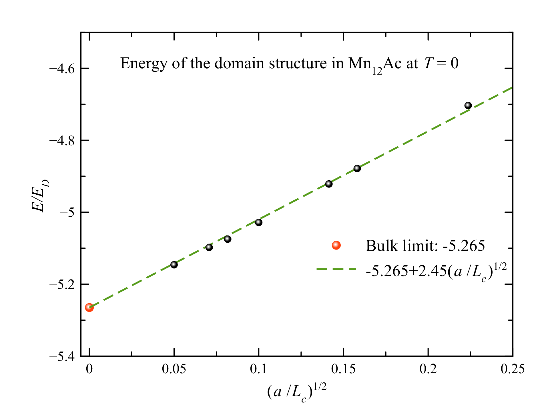
Figure 3: Dependence of the energy per magnetic molecule at $T=0$ on crystal length, showing the contribution of surfaces and domain walls.

With the conditional global dipolar-field updating, computation tends to be very fast at low temperatures because of the low acceptance rate. On the other hand, for a good system equilibration one needs a sufficient number of spin-flip acceptances. Thus the stopping/measuring strategy was modified as follows. The computation at a given temperature or bias field was stopped only after a certain fraction of acceptances per spin at high temperatures, $0.5\mathrm{NMC},$ was achieved. In most cases $0.2\times 0.5\mathrm{NMC}$ acceptances per spin was required. In the computation control program fulfillment of both criteria was required: equilibration and sufficient number of acceptances. The averaging interval was defined as the maximum of NMC updates and the last 1/4 of the actual number of spin updates, the latter becoming the case at low temperatures, exceeding NMC by far. Finally, the upper limit on the number of spin updates was set, typically 3000, to avoid getting stuck at the lowest temperatures.

Because of the global operation of computing the dipolar field, the computation is not fully parallelizable. Although the spin-update part can be parallelized, it does not make much sense because it is much faster than the global dipolar-field update even in its non-parallelized version.

Since the space-average magnetization in the domain state is zero, the domain order parameter

$$m_{D}=\sqrt{\left\langle\left(\frac{1}{N_{c}}\sum_{n_{c}=1}^{N_{c}}\sigma_{iz}\right)^{2}\right\rangle_{\mathrm{cols,}\mathrm{subs}}},$$ (30)

was computed for any state generated in the Monte Carlo routine and averaged over these states within the averaging interval. For all columns perfectly ordered, that is the case for a perfect domain state, one has $m_{D}=1$. For the completely disordered state, one has $m_{D}=1/N_{c}$, where $N_{c}=L_{c}/c$ is the number of magnetic molecules in the column.

Figure 4: Domains in the Mn₁₂Ac crystal of size $50\times 50\times 50$(70) at $T=0$ obtained by slow cooling, view along the $c$-axis. The plot was created using average spin polarization in $c$-columns.

Figure 5: Domains in the Mn₁₂Ac crystal of size $50\times 50\times 150$(210) at $T=0$ obtained by slow cooling, in the central $ac$ cross-section.

The reduced linear susceptibility $\tilde{\chi}$ can be computed either using the definition in Eq. (28) or using the formula

$$\tilde{\chi}=\frac{\left\langle m^{2}\right\rangle-\left\langle m\right\rangle^{2}}{\tilde{T}},\quad m\equiv\frac{1}{N}\sum_{i}\sigma_{iz},\quad\tilde{T}\equiv\frac{T}{E_{D}}.$$ (31)

The latter is not self-averaging for large system sizes and requires very long Monte Carlo sequences to average out fluctuations that is too costy for large systems.

V Numerical results

Results for the temperature dependence of the domain order parameter $m_{D}$ and the energy of box-shape Mn₁₂Ac crystals of different sizes obtained by lowering the temperature in small steps are shown in Fig. 2. For the largest crystal containing slightly above $10^{6}$ magnetic molecules, the computation requires about 30 hours. In accordance with the conclusion of the preceding section, the results depend only on the length of the crystal but not on its transverse dimensions. In the limit $T\rightarrow 0$ there are deviations of $m_{D}$ from the theoretical value 1 since column shapes do not fully equilibrate, especially for the longest crystal, so that domain walls are not everywhere parallel to the $c$-axis. Here annealing could help but it was not done.

The Curie temperature for the longest crystal is $T_{C}=0.36$ K, about two times lower than its mean-field value $0.707$ K. Such a big difference speaks of large critical fluctuations that can be expected in this quasi-one-dimensional systems with much stronger interaction within $c$-columns. The computed value of $T_{C}$ is very close to the experimentally measured value $T_{C}=0.34$ K for Fe₈ in Ref. burzurietal11prl . Since the two materials have comparable lattice parameters and the mean-field Curie temperature in Fe₈ is about 1 K, the close values of $T_{C}$ for the two materials are not surprizing. Fe₈ has even smaller ratio $T_{C}/T_{C}^{\mathrm{MFA}}$ that could be tentatively explained by the pyramidal shape of the crystals less favorable for ferromagnetic ordering. Unfortunately, this shape makes computation of the dipolar field in Fe₈ difficult.

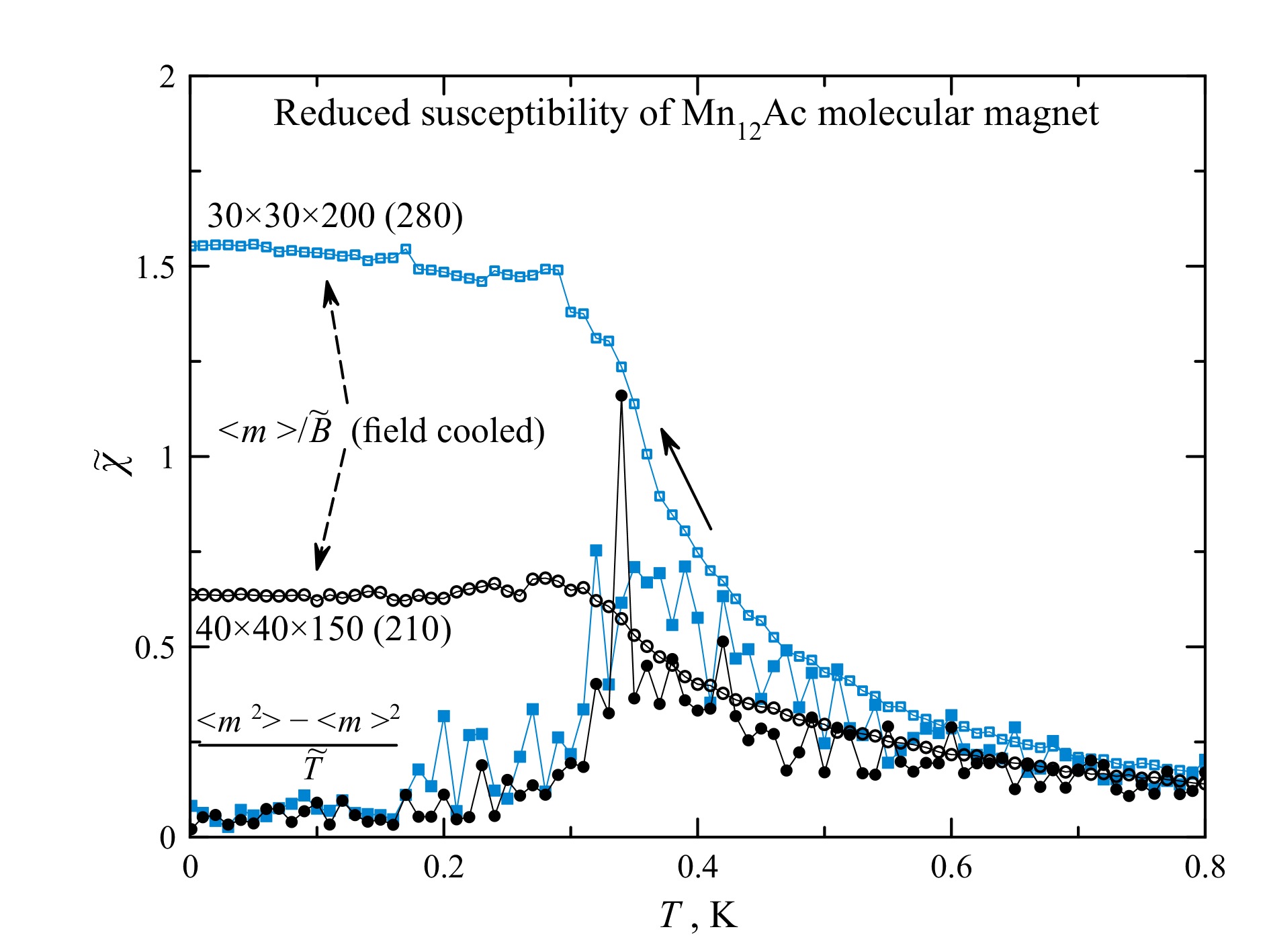
Figure 6: Reduced susceptibility of Mn₁₂Ac computed by two methods shows that domain walls are pinned at low temperatures.

Figure 7: Magnetization curves in Mn₁₂Ac (a): Hysteresis loop is vanishing with increasing temperature. (b) Equilibrium magnetization curves of Mn₁₂Ac with different transverse size of the crystal.

Fig. 3 confirms Eq. (24) for the contribution of the surface and domain walls to the energy and Eq. (7) in the bulk limit. By fitting one obtains $\delta E/E_{D}\simeq 2.45\sqrt{a/L_{c}}$. Since crystals used in the experiments are macroscopic, domains are large and the contribution of surfaces and walls into the energy is small.

Fig. 4 obtained by slow cooling the sample by step-wise lowering the temperature shows that domain walls are indeed diagonal, as suggested in Sec. III. For plotting, the average spin polarization in each column was used.

In Fig. 5 that provides a view onto the $ac$ cross-section with $n_{b}=N_{b}/2$, one can see that domains are parallel to the $c$-axis. At the ends of the crystal there is a little disturbance of the main structure that can be interpreted as domain branching.

The pattern of the dipolar field $D_{i,zz}$ is the same as that of $\sigma_{iz}$, so that figures such as Fig. 4 for these two quantities are indistinguishable. Domain walls are atomic-narrow, and on both sides of the wall $D_{i,zz}$ has its almost maximal positive or negative value created by the column of up or down spins. Since each spin, even adjacent to the wall, is polarized by a strong field, Monte Carlo spin flips are almost 100% rejected at low temperatures. This means that domain walls are pinned by the lattice and cannot easily move.

Lack of thermodynamic equilibrium at low temperatures is strikingly manifested in Fig. 6 showing reduced susceptibility computed by two different methods. Slow cooling in a small fixed magnetic field yields $\tilde{\chi}=\left\langle\sigma_{z}\right\rangle/\tilde{B}$ that increases with decreasing temperature and reaches a plateau. In computations, the value $\tilde{B}=0.1$ was used, so that the low-temperature magnetization $m=\tilde{\chi}\tilde{B}\approx 0.15$ is still far from saturation and the susceptibility should be close to linear. Computation with $\tilde{B}=0.03$ yields similar results with more scatter (not shown). From the plateau values one obtains $\tilde{\chi}L_{\bot}/L_{c}=0.23$ for the $30\times 30\times 200$ crystal and 0.17 for the $40\times 40\times 150$ crystal. These values qualitatively support Eq. (28). The low-temperature susceptibility could be interpreted as due to shiftifting of domain walls by the applied field, as in common ferromagnets. However, actual changing the field from zero to this value would result in a smaller and poorly defined value of $\tilde{\chi}$ because of domain-wall pinning and Barkhausen jumps. The true linear susceptibility is given by Eq. (31) and this one becomes small at low temperatures, that can be seen in Fig. 6 in spite of rather strong fluctuations that are very difficult to average out.

Another manifestation of domain-wall pinning is the hysteresis loop at $T=0$ seen in Fig. 7a. With increasing the temperature, this loop disappears. There is no loop at $T=0.3$ K and a narrow loop at $T=0.1$ K (not shown). Magnetization curves in Fig. 7b for crystals with different transverse sizes at $T=0.1$ K, still showing some hysteresis (only one branch shown), clearly scale with the transverse size in the horizontal direction, confirming Eqs. (28) and (29). Scaling and fitting magnetization curves, one obtains the numerical factor 0.12 in Eq. (28) that is of the same order of magnitude as found above.

VI Discussion

By slow cooling within the Monte Carlo method it was shown that Mn₁₂Ac orders ferromagnetically at 0.36 K into the ferromagnetic state with domains, extending findings of Ref. gar10prbrc where such type of ordering was obtained for much smaller crystals within the space-resolved mean-field approximation. Such a low value of $T_{C}$, two times lower than its mean-field value, is the consequence of the quasi-one-dimensional ordering dominated by columns of magnetic molecules along the $c$ axis. It was demonstrated that domains, being parallel to the $c$-axis, are separated by atomic-narrow domain walls whose cross-sections consist of diagonal lines in $ab$ planes, Fig. 4. Such narrow domain walls are pinned by the lattice at low temperatures.

It was shown that the period of the domain structure and the introduced here domain order parameter $m_{D}$ depend on the length of the crystal (in the $c$ direction) and do not depend on its transverse size. Magnetic susceptibility at low temperatures depends on crystal’s aspect ratio, Eq. (28), being large for prolate crystals.

In real Mn₁₂Ac spin transitions between up and down states are very slow at low temperatures, since they require spin tunneling under the energy barrier. Because of this, the crystal will not order spontaneously. Spin tunneling can be sped up and ordering can be facilitated if a strong magnetic field transverse to the anisotropy axes is applied. However, this can produce the undesirable bias because of the small misalignment of the anisotropy axes in different Mn₁₂Ac crystals. In this work, the effects of the energy barriers were not taken into account and a simple Ising-type model was adopted. Another molecular magnet Fe₈ is a better candidate for dipolar ordering because of the faster tunneling via transverse anisotropy, and the ordering was indeed observed by magnetic measurements at $T_{C}=0.34$ K, close to the value for Mn₁₂Ac found here. However, shapes of Fe₈ crystals are complicated and computation of dipolar fields is a more difficult problem.

References

- (1) J.R. Friedman, M.P. Sarachik, J. Tejada, R. Ziolo, Phys. Rev. Lett. 76, 3830 (1996)
- (2) J. Bartolomé, F. Luis, J.F. Fernández, eds., Molecular Magnets (Springer, 2014)
- (3) D.A. Garanin, E.M. Chudnovsky, Phys. Rev. B 78, 174425 (2008)
- (4) S. McHugh, R. Jaafar, M.P. Sarachik, Y. Myasoedov, H. Shtrikman, E. Zeldov, R. Bagai, G. Christou, Phys. Rev. B 79, 052404 (2009)
- (5) Y. Suzuki, M.P. Sarachik, E.M. Chudnovsky, S. McHugh, R. Gonzalez-Rubio, N. Avraham, Y. Myasoedov, E. Zeldov, H. Shtrikman, N.E. Chakov et al., Phys. Rev. Lett. 95, 147201 (2005)
- (6) D.A. Garanin, E.M. Chudnovsky, Phys. Rev. B 76, 054410 (2007)
- (7) D.A. Garanin, Phys. Rev. B 88, 064413 (2013)
- (8) J.F. Fernández, J.J. Alonso, Phys. Rev. B 62, 53 (2000)
- (9) X.M. Hidalgo, E.M. Chudnovsky, A. Aharony, Europhys. Lett. 55, 273 (2001)
- (10) F. Luis, J. Campo, J. Gómez, G.J. McIntyre, J. Luzón, D. Ruiz-Molina, Phys. Rev. Lett. 95(22), 227202 (2005)
- (11) M. Evangelisti, A. Candini, A. Ghirri, M. Affronte, G.W. Powell, I.A. Gass, P.A. Wood, S. Parsons, E.K. Brechin, D. Collison et al., Phys. Rev. Lett. 97(16), 167202 (2006)
- (12) A. Morello, F.L. Mettes, O.N. Bakharev, H.B. Brom, L.J. de Jongh, F. Luis, J.F. Fernández, G. Aromí, Phys. Rev. B 73(13), 134406 (2006)
- (13) A.J. Millis, A.D. Kent, M.P. Sarachik, Y. Yeshurun, Phys. Rev. B 81(2), 024423 (2010)
- (14) B. Wen, P. Subedi, L. Bo, Y. Yeshurun, M.P. Sarachik, A.D. Kent, A.J. Millis, C. Lampropoulos, G. Christou, Phys. Rev. B 82(1), 014406 (2010)
- (15) D.A. Garanin, Phys. Rev. B 81(22), 220408 (2010)
- (16) E. Burzurí, F. Luis, B. Barbara, R. Ballou, E. Ressouche, O. Montero, J. Campo, S. Maegawa, Phys. Rev. Lett. 107, 097203 (2011)