The Origin of the Iron-Rich Knot in Tycho’s Supernova Remnant

Abstract

X-ray observations of supernova remnants (SNRs) allow us to investigate the chemical inhomogeneity of ejecta, offering unique insight into the nucleosynthesis in supernova explosions. Here we present detailed imaging and spectroscopic studies of the “Fe knot” located along the eastern rim of the Type Ia SNR Tycho (SN 1572) using Suzaku and Chandra long-exposure data. Surprisingly, the Suzaku spectrum of this knot shows no emission from Cr, Mn, or Ni, which is unusual for the Fe-rich regions in this SNR. Within the framework of the canonical delayed-detonation models for SN Ia, the observed mass ratios $M_{\rm Cr}/M_{\rm Fe}<0.023$, $M_{\rm Mn}/M_{\rm Fe}<0.012$, and $M_{\rm Ni}/M_{\rm Fe}<0.029$ (at 90% confidence) can only be achieved for a peak temperature of (5.3–5.7) $\times 10^{9}$ K and a neutron excess of $\lesssim 2.0\times 10^{-3}$. These constraints rule out the deep, dense core of a Chandrasekhar-mass white dwarf as the origin of the Fe knot, and favors either incomplete Si burning or the $\alpha$-rich freeze-out regime, probably close to their boundary. An explosive He burning regime is a possible alternative, although this hypothesis is in conflict with the main properties of this SNR.

1. Introduction

Type Ia supernovae (SNe Ia), widely believed to originate from thermonuclear explosions of white dwarfs, play an important role in the chemical evolution of the universe, as they release a large amount of heavy elements synthesized during the explosion. SNe Ia are also crucial for the study of cosmology, owing to their use as distance indicators. Nevertheless, many of their fundamental aspects still remain poorly understood (e.g., Maoz et al. 2014).

X-ray observations of supernova remnants (SNRs) provide unique insight into the nucleosynthesis that had taken place in their progenitor, because they allow us to investigate the amount and distribution of heavy elements via spatially-resolved spectral analysis (e.g., Hwang & Laming 2012; Park et al. 2007). Tycho’s SNR, the remnant of SN 1572, is an ideal object in that sense, since its spatial structure is well resolved owing to its proximity and moderate angular size (e.g., Decourchelle et al. 2001; Warren et al. 2005). Tycho’s SNR is thought to be the result of a typical SN Ia explosion with a normal brightness that synthesized $\sim$ 0.7$M_{\odot}$ of ⁵⁶Ni, based on spectroscopy of the optical light echo (Krause et al. 2008) and an X-ray study combined with hydrodynamical simulations (Badenes et al. 2006).

The chemical inhomogeneity in Tycho’s SNR has been studied extensively. ASCA observations revealed a stratified elemental composition throughout most of the SNR, with Fe interior to the intermediate-mass elements (IMEs: e.g., Si, S, Ar, Ca) (Hwang & Gotthelf 1997; Hwang et al. 1998). This stratification is consistent with predictions from modern numerical simulations (e.g., Seitenzahl et al. 2013b) as well as actual observations of an SN Ia explosion (e.g., Mazzali et al. 2007; Tanaka et al. 2011). On the other hand, the eastern region of the SNR exhibits somewhat unusual morphological features: several ‘clumps’ overrunning the forward shock have been spatially resolved (Vancura et al. 1995, see also Figure 1). Given the enhanced abundance of Fe confirmed by XMM-Newton (Decourchelle et al. 2001), one of the clumps (hereafter “Fe knot”) is likely to have originated from a relatively hot region in the exploding progenitor, where a large amount of ⁵⁶Ni was generated. Interestingly, the location of the Fe knot coincides with an apparent ‘gap’ in the reverse shock structure identified by Chandra (Warren et al. 2005). This coincidence suggests an association between the mechanism that created the Fe knot and the bulk dynamics of the explosion. However, to date there has been no extensive investigation of the nature of this interesting knot based on an X-ray spectroscopy.

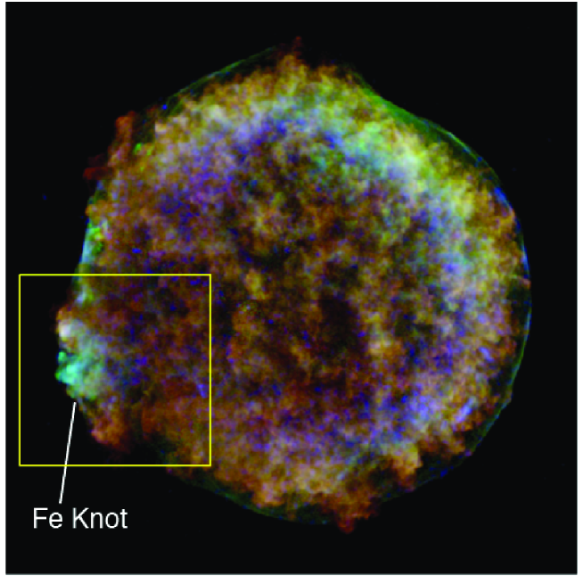
Figure 1.— Three-color image of Tycho’s SNR from the Chandra deep observation. Red, green, blue are emission from the Si K (1.8–1.92 keV), Fe L (0.8–1.25 keV), and Fe K (6.35–6.6 keV) bands, respectively. The yellow box indicates the region shown in Figure 8.

More recently, Suzaku has opened a new window into the physics of both SNe Ia and their remnants with its high sensitivity for weak lines, such as K$\alpha$ emission of the secondary Fe-peak elements (e.g., Cr, Mn, Ni, which are normally synthesized together with Fe) and K$\beta$ fluorescence of Fe (e.g., Tamagawa et al. 2009; Yang et al. 2013; Yasumi et al. 2014). For instance, the abundances of the secondary Fe-peak elements provide a probe of the neutron excess in the progenitor, due to either metallicity effects (Badenes et al. 2008; Park et al. 2013) or electron capture reactions during the SN explosion (Yamaguchi et al. 2015). The centroid energy and intensity of the Fe K$\beta$ fluorescence, on the other hand, constrain the physical conditions in the non-equilibrium plasma (Yamaguchi et al. 2014b), which in turn enables accurate abundance measurements to be made. In this paper, we perform detailed imaging spectroscopy of Tycho’s Fe knot utilizing both the superior sensitivity of Suzaku and the excellent angular resolution of Chandra, and place strong constraints on its plasma state and origin.

Throughout this paper, the distance to the SNR is assumed to be 3 kpc (e.g., Ruiz-Lapuente 2004; Tian & Leahy 2011), but our main results and conclusions are not affected by its exact value (see Hayato et al. 2010, for its systematic uncertainty from various literatures). The spectral analysis is all performed with the XSPEC software (Arnaud 1996). The errors quoted in the text and table represent the 90% confidence level, and the error bars given in the spectra represent 1$\sigma$ confidence.

2. Observational Results

We analyzed archival data of Tycho’s SNR obtained using the Suzaku X-ray Imaging Spectrometer (XIS) and the Chandra Advanced CCD Imaging Spectrometer (ACIS), the same datasets as used by Yamaguchi et al. (2014b) and Eriksen et al. (2011), respectively. The details of the observations are summarized in Table 1. We reprocessed the data in accordance with the standard procedures using the latest calibration database, obtaining the total effective exposures given also in Table 1. Figure 1 shows an ACIS high-resolution image of Tycho’s SNR, where the Fe knot at the eastern rim is indicated.

Table 1Summary of the Observations.

Missions	Suzaku	Chandra
Instruments	XIS0 & 3	ACIS-I
Cycle	3 (LP∗)	10 (LP∗)
Observation ID	5030850[1,2]0	1009[3–7], 1090[2–4,6]
Observation Date	2008 Aug 4–12	2009 Apr 11–May 3
Exposure Time (ks)	416	734

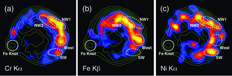
Figure 2.— Suzaku/XIS smoothed images of Tycho’s SNR in the 5.38–5.58 keV (a: Cr K$\alpha$), 7.00–7.20 keV (b: Fe K$\beta$), and 7.38–7.58 keV (c: Ni K$\alpha$) bands where a 6.34–6.53 keV (Fe K$\alpha$) image is overplotted in contours. The continuum flux estimated using a 7.7–9.0 keV image is subtracted from the raw images. The white solid circle is where an XIS spectrum of the Fe knot (Figure 3) is extracted. We also extract spectra from the other regions enclosed by the dashed circles or ellipses for comparison, which are shown in Figure 4.

2.1. Suzaku Narrow Band Images

Figure 2 shows Suzaku/XIS images of the SNR at the energies of (a) Cr K$\alpha$, (b) Fe K$\beta$, and (c) Ni K$\alpha$ emission, after subtracting the nonthermal continuum flux estimated using the procedure described in Yamaguchi et al. (2014b). We use only the data from the front-illuminated CCDs (XIS0 and 3) and merge them to improve the photon statistics. The green contours overlaid on the images are taken from the Fe K$\alpha$ band, where the Fe knot is clearly seen at the east rim even with the lower angular resolution of the XIS images. No counterpart of the Fe knot is apparent in any of the other energy bands (i.e., Cr K$\alpha$, Fe K$\beta$, and Ni K$\alpha$). Although the primary topic of this paper is the Fe knot, we here briefly comment on other interesting features revealed by Figure 2. There is a distinct difference in the distribution of Cr and Fe (with the former at a larger radius) along the western side. This separation supports the idea suggested by Badenes et al. (2008) that the shocked Cr originates from explosive Si burning, whereas Fe comes from a mixture of Si burning and nuclear statistical equilibrium (NSE) burning. The even smaller peak radius of the Fe K$\beta$ emission at the bright northwest (NW) region is due to the extremely low ionization of the ejecta immediately behind the shock (Yamaguchi et al. 2014b). A second peak in the Fe K$\beta$ image is found along the western rim, where the lowest ambient density is reported (Williams et al. 2013). Although the detailed morphology of the Ni K$\alpha$ emission can provide important clues to SN Ia explosion physics (as we discuss is §3), the photon statistics in Figure 2(c) are too poor to allow us to conclude anything about the actual Ni distribution in Tycho’s SNR. More detailed study of these features is left for future work.

2.2. Spectrum Extraction and Comparison

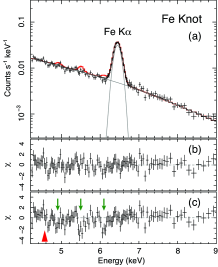
Figure 3.— (a) An XIS spectrum of the Fe knot in 4.2–9.0 keV. Besides the strong Fe K$\alpha$ line, no significant line emission is detected. The red line shows the model reported by Miceli et al. (2015) where detection of Ti (at $\sim$4.9 keV), Cr, and Mn K$\alpha$ lines was claimed.  (b) Residuals from our best-fit model consisting of only one Gaussian for the Fe K$\alpha$ and a power-low for the continuum component. (c) Residuals from the model of Miceli et al. (2015). Dips are seen at the energies of the claimed lines (green arrows). The Ti K$\alpha$ centroid expected for the ionization timescale of the Fe knot ($n_{e}t\sim 1.2\times 10^{10}$ cm^-3 s) is indicated by the red triangle in panel(c). See §2.4 for more details.

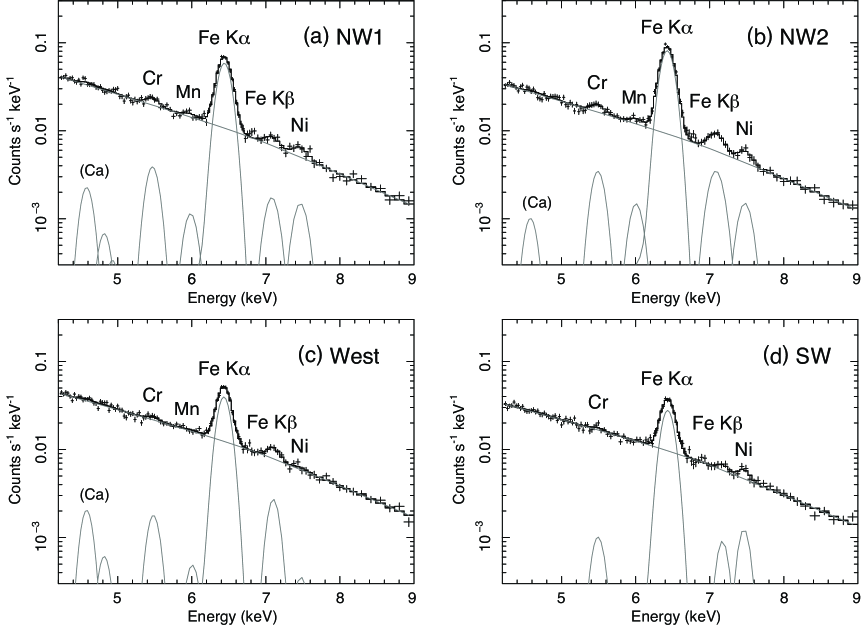
Figure 4.— XIS spectra of the (a) NW1, (b) NW2, (c) West and (d) SW regions given in Figure 2. The phenomenological model components (a power law and Gaussians) applied to determine the line parameters are shown as well.

For more quantitative studies, we extract an XIS spectrum of the Fe knot from the region in Figure 2 marked by a circle at (R.A., Dec.)_J2000 = (0h 25m 52.5s, +64^∘07^′10.$\!{}^{\prime\prime}$0) with a diameter of 1.$\!{}^{\prime}$5. Since this value is smaller than the half-power diameter (HPD) of the Suzaku X-Ray Telescope (XRT: $\sim$ 2.$\!{}^{\prime}$0; Serlemitsos et al. 2007), we study the effect of photon scattering using the xissim task with the Chandra image at the Fe-K band as an input. We find that about 35% of photons originating from the Fe knot are detected in the circular region (i.e., the remaining 65% fell into the outer regions), but this detector region is still dominated by the photons from the Fe knot itself. A spectrum of the non-X-ray background (NXB) for the same detector region is generated using the XIS night-Earth database and subtracted from the source spectrum. The resulting spectrum in the 4.2–9.0 keV band is shown in Figure 3(a). We find that the continuum level of the NXB is $\sim 4\times 10^{-5}$ counts s^-1 keV^-1, well below the source spectrum. Therefore, a high signal-to-noise ratio is achieved in this region. We ignore the contribution of the cosmic X-ray background (CXB), since its flux is less than 1% of the source even at $\sim$ 9 keV where the estimated CXB/source flux ratio would be highest. Although K$\alpha$ emission lines from the secondary Fe-peak elements, as well as Fe K$\beta$ fluorescence, fall in this energy band (4.2–9.0 keV), we see no evidence for them. For comparison, we also extract spectra from other regions (dashed circles or ellipses given in Figure 2) in Figure 4. The regions are chosen to contain bright spots of either Cr K$\alpha$, Fe K$\beta$, or Ni K$\alpha$ emission. Despite the significantly higher continuum level in these spectra than in the Fe knot region, they clearly show weak lines associated with these metal species. This indicates that the absence of these lines in the Fe knot spectrum is not due to insufficient energy resolution or photon statistics but indeed is due to their low line fluxes.

We fit all the spectra (Figure 3 and 4) with ad hoc Gaussian models to constrain the line centroids and flux ratios relative to Fe K$\alpha$. The line widths of the weak or undetected lines are linked to that of the Fe K$\alpha$ line. The results are given in Table 2, where the flux upper limit for the undetected lines is determined using the procedures described in §2.3 and §2.4. The flux ratios are generally in good agreement with the imaging analysis; for instance, the NW1 region (brightest in the Cr K$\alpha$ image) has the highest Cr/Fe ratio. Interestingly, the Fe K$\alpha$ centroid energy of the Fe knot is highest among the analyzed regions, indicating that the Fe ejecta in this SNR are most highly ionized in the Fe knot. During the spectral fitting performed above, we model the continuum component with a power law, assuming absorption by the foreground interstellar medium (ISM) by a hydrogen column density of $7\times 10^{21}$ cm^-2 (Cassam-Chenaï et al. 2007) and standard ISM abundances (Wilms et al. 2000). We also take into account the contribution of K$\beta$ and K$\gamma$ emission of He-like Ca by fixing their centroids and flux ratios at the theoretical values, although this does not affect the results we obtain.

Table 2Statistics and best-fit parameters for the Suzaku spectra.

	Fe Knot	NW1	NW2	West	SW
Photon Counts
4.2–9.0 keVa	14390	32906	31104	33422	25372
Fe K$\alpha$b	3050	5612	7881	3598	2557
Centroids [eV]
Cr K$\alpha$	(5480–5490)c	$5474_{-29}^{+27}$	$5497_{-34}^{+29}$	$5487\pm 53$	$5496_{-86}^{+88}$
Mn K$\alpha$	(5952–5960)c	$5989_{-78}^{+105}$	$6012\pm 65$	6012	6012
Fe K$\alpha$	$6453_{-4}^{+3}$	$6445\pm 3$	$6433_{-3}^{+2}$	$6438_{-3}^{+4}$	$6437\pm 4$
Fe K$\beta$	(7100–7400)	$7087_{-40}^{+46}$	$7091\pm 23$	$7107_{-27}^{+29}$	$7176_{-60}^{+58}$
Ni K$\alpha$	(7509–7514)c	$7473_{-50}^{+47}$	$7482_{-39}^{+38}$	7482	$7467_{-35}^{+40}$
Flux Ratios [%]
Cr/Fe (K$\alpha$)	$<$ 2.5d	$5.6\pm 1.6$	$3.6_{-1.0}^{+1.1}$	$3.8\pm 2.4$	$3.1\pm 2.9$
Mn/Fe (K$\alpha$)	$<$ 1.0d	$1.8\pm 1.4$	$1.7\pm 0.9$	$1.1_{-1.1}^{+2.1}$	$0.1_{-0.1}^{+2.5}$
Fe K$\beta$/K$\alpha$	$<$ 2.3d	$3.7\pm 1.3$	$5.7_{-1.2}^{+1.4}$	$7.6_{-2.2}^{+2.6}$	$3.6\pm 2.4$
Ni/Fe (K$\alpha$)	$<$ 2.6d	$3.8\pm 1.4$	$2.7\pm 0.9$	$1.3_{-1.3}^{+2.1}$	$5.6\pm 2.5$

2.3. Plasma Diagnostics for the Fe Knot

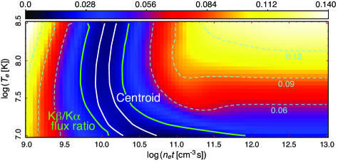
Figure 5.— Theoretical predictions for the Fe K$\beta$/K$\alpha$ emissivity ratio as a function of the ionization timescale ($n_{e}t$: horizontal axis) and electron temperature ($T_{e}$: vertical axis). The regions constrained by the observed flux ratio and Fe K$\alpha$ centroid are indicated by the green and white curves, respectively. To derive the latter, Figure 3(c) of Yamaguchi et al. (2015) is used with account of the systematic uncertainty in the detector gain (0.1% of the mean energy; Ozawa et al. 2009). Note that the emissivity ratio is lowest around the constrained ionization timescale ($\sim 1\times 10^{10}$ cm^-3 s), because the dominant Fe ions at this plasma condition (Fe¹⁶⁺ and Fe¹⁷⁺) still have many $2p$ electrons but no $3p$ electron that is responsible for the K$\beta$ fluorescence.

The Fe K$\alpha$ centroid of the Fe knot ($6453_{-4}^{+3}$ eV) corresponds to an average charge number of $\left<z_{\rm Fe}\right>=17$ (Yamaguchi et al. 2014b). Also sensitive to the Fe charge number is the K$\beta$/K$\alpha$ flux ratio, because the fluorescence yields of these lines depend on the number of bound electrons in the $2p$ and $3p$ shells. We find that this ratio for the Fe knot does not exceed 0.023 (at the 90% confidence level) for any K$\beta$ centroid energy between 7.1 keV to 7.4 keV. Figure 5 shows the theoretically-predicted Fe K$\beta$/K$\alpha$ emissivity ratio as a function of the ionization timescale (horizontal axis) and electron temperature (vertical axis), calculated using the latest AtomDB database (see also Yamaguchi et al. 2015), where the ionization timescale $n_{e}t$ is the product of the electron density and the elapsed time since the gas was shock heated. The regions constrained by the measured flux ratio and the K$\alpha$ centroid are fully consistent with each other (Figure 5). This consistency indicates that the Fe K-shell spectrum of this knot is well characterized by a non-equilibrium ionization (NEI) plasma model with a single ionization timescale of $\sim 1.2\times 10^{10}$ cm^-3 s, supporting the idea that the Fe knot is indeed an isolated ejecta clump, in contrast to the Fe ejecta in the main SNR shell where a broad range of ionization states has been measured (Yamaguchi et al. 2014b).

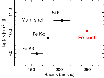
Figure 6.— Relationship between the ionization timescale and the distance from the SNR center for the Fe knot (red) and the bulk emission from the main SNR shell (black), clearly showing that the Fe knot is dynamically distinct from the bulk of the ejecta. The SNR center determined from previous Chandra observations (Warren et al. 2005) is assumed.

The different thermodynamic evolution of the Fe knot is illuminated more clearly in Figure 6, where its angular radius and ionization timescale are compared with those of the main SNR shell (i.e., bright NW region). We choose Si K, Fe K$\alpha$, and Fe K$\beta$ as the characteristic emission from the bulk of the ejecta, and plot (with the black points) their radial extent and ionization timescale reported in previous work (Warren et al. 2005; Badenes et al. 2007; Yamaguchi et al. 2014b). The figure indicates that the exterior ejecta tend to be more highly ionized at the main SNR shell, as naturally expected from the reverse shock dynamics (e.g., Badenes et al. 2003), while the Fe knot (the red point) is distinctly inconsistent with the trend.

2.4. Searching for the Low-Abundance Elements

The plasma state of the Fe knot constrained by our diagnostics predicts centroid energies of the Cr, Mn, and Ni K$\alpha$ emission to be 5480–5490 eV, 5952–5960 eV, and 7509–7514 eV, respectively. Allowing the line centroid to vary within these ranges, we derive their flux upper limits relative to Fe K$\alpha$ as given in Table 2. Miceli et al. (2015) recently reported that the largest equivalent width (EW) of the Cr K$\alpha$ line in this SNR is found at the Fe knot, based on their analysis of XMM-Newton/EPIC data. We constrain, however, the Cr/Fe EW ratio to $<$ 0.016, ruling out their detection ($0.033\pm 0.015$). Although the HPD of the Suzaku/XRT is larger than that of XMM-Newton and thus some photons from the Fe knot are lost, this does not affect the line flux ratios because the XRT point spread function is almost independent of the X-ray energy (Serlemitsos et al. 2007). Moreover, even if some photons from the outer regions with a ‘normal’ Cr/Fe ratio contribute to the Fe knot spectrum, this would rather increase the XIS-measured Cr/Fe ratio. We therefore consider that the lack of Cr emission in the Fe knot is robust. Miceli et al. (2015) also reported the detection of Ti and Mn K$\alpha$ lines from this region (though the latter is marginal). In Figure 3(a), we show their best-fit model (normalized to the XIS spectrum) with the red line, where the EW (or flux) ratios among the lines they reported are assumed. Figure 3(b) and 3(c) show the residuals for our best-fit and Miceli et al.’s models, respectively. The latter clearly shows negative residuals at each line energy. We confirm that the addition of any lines significantly increases the $\chi^{2}$ value (e.g., from 99 to 116 for Mn K$\alpha$, with 106 degrees of freedom).

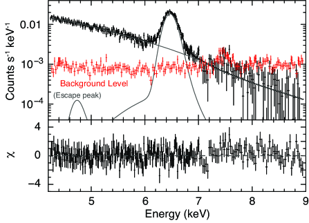
Figure 7.— Chandra/ACIS spectrum of the entire Fe knot in the 4.2–9.0 keV band (black), fitted with a model consisting of a Gaussian (for the Fe K$\alpha$ emission) and a power low (for the continuum). The red data points are the background spectrum for the knot region, indicating that the source spectrum above 7 keV is dominated by the background in the ACIS data. The structure around 4.8 keV of the model (gray line) is a Si-escape peak of the Fe K$\alpha$ component (detector origin). The bottom panel shows the residual between the data and model.

We also analyze the Chandra/ACIS data to check the consistency. Figure 7 shows an ACIS spectrum in the 4.2–9.0 keV band extracted from the entire Fe knot (yellow ellipse in Figure 8). A background spectrum is taken from a nearby region in the same CCD chip, which is also shown in Figure 7. Despite the relatively high background level (compared to the XIS), the obtained photon statistics are still high enough at the energies below 7 keV, owing to the longer exposure and smaller photon-escape effect. We see, however, no clear feature of Cr or Mn K$\alpha$ emission. The upper limit of the Cr/Fe EW ratio is obtained to be 0.009 (and the flux ratio is $<$ 0.028), again, ruling out the XMM-Newton result. Note that the total effective exposure of the XMM-Newton data (Miceli et al. 2015) was only $\sim$ 125 ks, and they analyzed only EPIC-pn spectra, of which instrumental background contains Cr fluorescence lines and is largely position dependent. Incomplete background subtraction may explain their detection of a Cr line. Our analysis is based on the XIS-FI data with the lowest, stable background level plus the best available energy resolution, together with the ACIS deep observations. The result is therefore considered to be more reliable than any previous measurements.

The detection of a Ti line is also questionable from a theoretical consideration. While the reported centroid of $\sim$ 4.93 keV corresponds to the Ly$\alpha$ line of H-like Ti, based on the plasma conditions in the Fe knot ($n_{e}t\approx 1.2\times 10^{10}$ cm^-3 s) the Ti K$\alpha$ centroid is expected to be $\sim$ 4.59 keV (indicated by the red triangle in Figure 3(c)). Since the majority of the ejecta in Tycho’s SNR is in the He-like or even lower charge states (e.g., Badenes et al. 2006; Yamaguchi et al. 2014a), it is unlikely that only Ti is in the highly-ionized H-like state. Further studies might be required to conclude how this possibly artificial 4.9-keV line is formed.

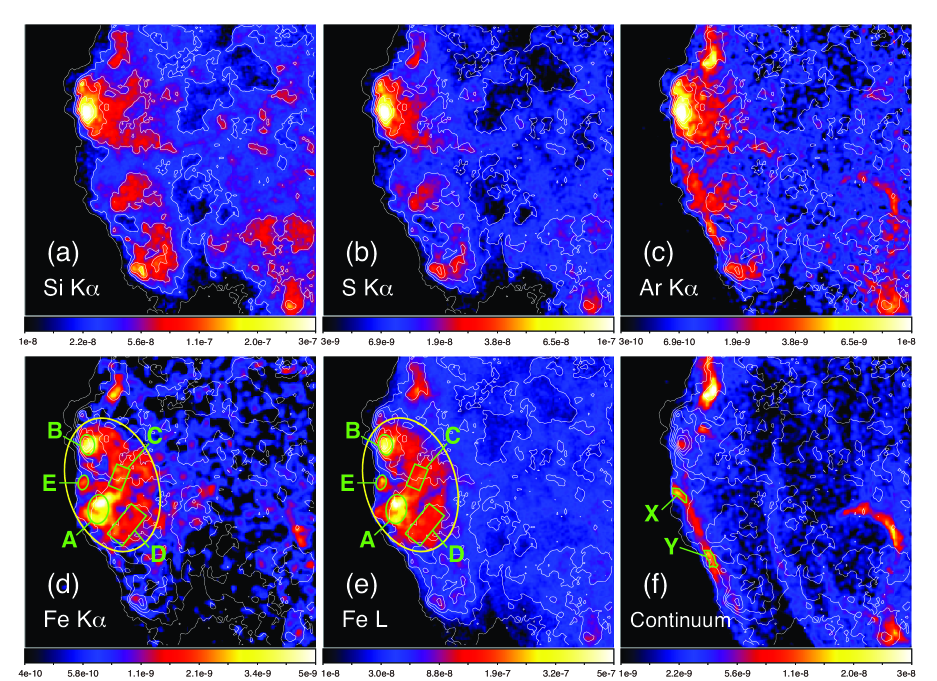
Figure 8.— Chandra/ACIS images of the eastern region of Tycho’s SNR (the yellow square in Figure 1) containing the Fe knot. The energy band of each panel is following: (a) 1.8–1.92 keV, (b) 2.4–2.52 keV, (c) 3.07–3.18 keV, (d) 6.35-6.6 keV, (e) 0.8–1.25 keV, and (f) 4.2–6.0 keV. The unit of the color bar values is photons cm^-2 s^-1. The contours for the 1.80–1.92 keV (Si K$\alpha$) emission are overlaid on all the images. The yellow ellipse encloses the entire Fe knot. The spectra from the smaller regions (green) are analyzed in detail in §2.6.

2.5. Chandra High-Resolution Images

In Figure 8, we show narrow band ACIS images of the region around the Fe knot at the energies of (a) Si K$\alpha$, (b) S K$\alpha$, (c) Ar K$\alpha$, (d) Fe K$\alpha$, (e) Fe XVII–XIX L-shell blend, and (f) 4.2–6.0 keV continuum emission. Each image is overplotted with the contours of the Si K$\alpha$ emission. The surface brightness distribution of the Si, S, and Ar K$\alpha$ emission (i.e., the IMEs) is quite similar to one another. On the other hand, the Fe emission (both K$\alpha$ and L-shell blend) exhibits a distinctly different morphology from that of the IMEs. A thin filamentary feature found in the continuum band is similar to the nonthermal rims seen elsewhere in this remnant and suggests that we are seeing the forward shock projected on the Fe knot emission.

Table 3Fe K$\alpha$ flux and size of each subregion.

Knot	Fe K$\alpha$ flux	Angular size		Volume
	[$10^{-6}$ ph cm-2 s-1]	[arcsec2]	[pc2]	[$10^{54}$ cm3]
A	$4.58\pm 0.41$	231	0.0486	1.00
B	$1.94\pm 0.28$	113	0.0239	0.494
C	$1.79\pm 0.25$	160	0.0338	0.698
D	$3.03\pm 0.33$	364	0.0770	1.59
E	$0.54\pm 0.19$	57.1	0.0121	0.250
Total∗	$35.2\pm 1.2$	4820	1.01	21.0

Based on its morphology, the Fe knot can be divided into substructures. The brightest spot, indicated as “A” in Figure 8(d) or 8(e), is found near the middle of the Fe knot. This feature seems physically distinct from the surrounding IME blobs. The second brightest peak “B”, on the other hand, spatially coincides with the IME emission. The other subregions, “C”, “D”, and “E”, are also bright in the Fe bands but not associated with the morphology of the IMEs. In short, only Knot B may have a different chemical composition from the others. The Fe K$\alpha$ line flux from and physical size of each subregion are listed in Table 3. The emitting volume (also given in Table 3) is roughly estimated assuming a plasma depth of 0.7 pc, which corresponds to an angular size of $48^{\prime\prime}$ at the nominal distance of 3 kpc. Readers should be warned that this depth and thus the estimated volume have relatively large uncertainty. The average surface brightness of the Fe K$\alpha$ emission in the whole Fe knot (yellow ellipse in Figure 8) is $7.3\times 10^{-9}$ photons cm^-2 s^-1 arcsec^-2, about 37% of that at the brightest Knot A.

2.6. Small-Scale Spectra

An ACIS spectrum from each subregion is extracted and shown in Figure 9, where a background taken from the same CCD chip is subtracted. We also extract nonthermal spectra from the regions “X” and “Y” in Figure 8(f) to investigate the characteristic continuum shape (i.e., photon index) of spectra around the knot. We fit these nonthermal spectra with an absorbed power law plus a pure-metal NEI model (see below for details) with free abundances of Si, S, Ar, and Fe that appear in the spectra. We obtain $N_{\rm H}$ = $7.9_{-0.7}^{+0.9}\times 10^{21}$ cm^-2 and $\Gamma$ = 2.58 $\pm$ 0.06 for Region X, and $N_{\rm H}$ = $9.4_{-1.2}^{+0.9}\times 10^{21}$ cm^-2 and $\Gamma$ = $2.68_{-0.08}^{+0.07}$ for Region Y. Both parameters overlap between the two regions, and are consistent with the typical values in this SNR (Cassam-Chenaï et al. 2007).

Figure 10 shows the background-subtracted spectrum of Knot A, the same as shown in Figure 9. No feature of Cr, Mn, or Ni emission is confirmed in this spectrum. Owing to the relatively small amount of contamination from the IME component in this subregion (see Figure 8), we see prominent features of the L-shell blend of Fe XVII, Fe XVIII, and Fe XIX at $\sim$ 0.83 keV ($3d$$\rightarrow$$2p$) and $\sim$ 1.1 keV (transitions from $n\geq 4$ to $n=2$). This indicates that the L-shell emission from the Fe knot is dominated by Ne-like and F-like Fe, consistent with the origin of the Fe K$\alpha$ fluorescence (§2.3). The identical origin of the Fe L and K$\alpha$ emission is also implied from their similar morphology as seen in Figure 8(d) and 8(e). This result allows us to determine the characteristic electron temperature of the Fe knot using the L-shell/K-shell flux ratio, because their line emissivities strongly depend on the internal energy (i.e., temperature) of free electrons.

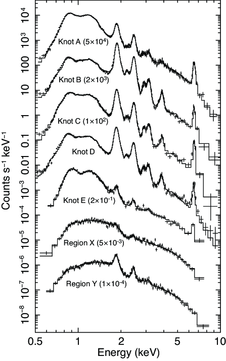
Figure 9.— ACIS spectra (background subtracted) taken from the small regions given in Figure 8. The normalization of each spectrm is adjusted by multiplying the factor given in the panel.

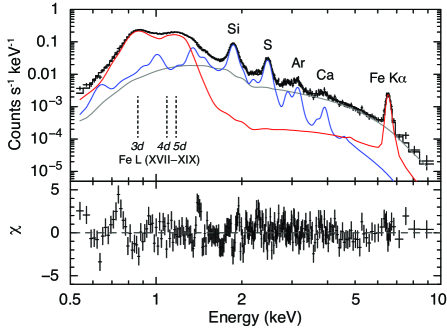
Figure 10.— The ACIS spectrum of Knot A. The best-fit models for the Fe knot, IME, and power-law components are given in the red, blue, and gray lines, respectively. The bottom panel shows the residual between the data and model.

Table 4The best-fit spectral parameters for Knot A.

Components	Parameters	Values
Absorption	$N_{\rm H}$ [$10^{21}$ cm-2]	$8.1\pm 0.1$
Fe knot	$kT_{e}$ [keV]	$8.1_{-0.4}^{+0.6}$
(low-$n_{e}t$)	$n_{e}t$ [$10^{10}$ cm-3 s]	$1.26\pm 0.02$
	$n_{e}n_{\rm Fe}V$ [$10^{51}$ cm-3]	$3.93\pm 0.03$
IME	$kT_{e}$ [keV]	$1.5_{-0.1}^{+0.3}$
(high-$n_{e}t$)	$n_{e}t$ [$10^{10}$ cm-3 s]	$5.42_{-0.55}^{+0.21}$
	$n_{e}n_{\rm Si}V$ [$10^{51}$ cm-3]	$3.49_{-0.04}^{+0.05}$
	$n_{\rm Ne}/n_{\rm Si}$	$0.98\pm 0.09$
	$n_{\rm Mg}/n_{\rm Si}$	$0.49\pm 0.02$
	$n_{\rm S}/n_{\rm Si}$	$0.65\pm 0.03$
	$n_{\rm Ar}/n_{\rm Si}$	$0.13\pm 0.02$
	$n_{\rm Ca}/n_{\rm Si}$	$0.11\pm 0.04$
Power law	$\Gamma$	$2.62_{-0.04}^{+0.03}$
	Normalizationa	$3.20_{-0.70}^{+0.83}$
$\chi^{2}/d.o.f$		380/228

Table 5The best-fit parameters for the Chandra spectra of the Fe knot subregions.

I. Nonthermal continuum model
Knot	$N_{\rm H}$	$kT_{e}$ (Fe)	$n_{e}t$ (Fe)	$n_{e}n_{\rm Fe}V$	$kT_{e}$ (IME)	$n_{e}t$ (IME)	$n_{e}n_{\rm Si}V$	$\Gamma$	$\chi^{2}$/d.o.f.	$\chi^{2}$/d.o.f.
	[$10^{21}$ cm-2]	[keV]	[$10^{10}$ cm-3 s]	[$10^{51}$ cm-3]	[keV]	[$10^{10}$ cm-3 s]	[$10^{51}$ cm-3]		(Full band)a	(Fe L/K)b
A	$8.1\pm 0.1$	$8.1_{-0.4}^{+0.6}$	$1.26\pm 0.02$	$3.93\pm 0.03$	$1.5_{-0.1}^{+0.3}$	$5.42_{-0.55}^{+0.21}$	$3.49_{-0.04}^{+0.05}$	$2.62_{-0.04}^{+0.03}$	380/228	76/67
B	$6.8\pm 0.1$	$8.9_{-0.4}^{+0.2}$	$1.01_{-0.02}^{+0.03}$	$1.35_{-0.03}^{+0.01}$	$14\pm 0.8$	$1.74\pm 0.02$	$8.32_{-0.04}^{+0.08}$	$2.85_{-0.05}^{+0.07}$	1080/207	68/47
C	$8.5\pm 0.1$	$8.6_{-0.8}^{+0.3}$	$1.33\pm 0.02$	$1.57_{-0.02}^{+0.03}$	$1.5\pm 0.1$	$5.21_{-0.16}^{+0.30}$	$5.02_{-0.07}^{+0.05}$	$2.62_{-0.08}^{+0.12}$	336/163	48/43
D	$6.5\pm 0.1$	$8.6_{-0.3}^{+0.2}$	$1.06\pm 0.02$	$2.06\pm 0.02$	$1.4\pm 0.1$	$5.03_{-0.15}^{+0.11}$	$13.9\pm 0.1$	$2.62\pm 0.04$	812/224	125/58
E	$8.5\pm 0.7$	$6.0_{-1.4}^{+2.0}$	$1.59\pm 0.06$	$0.61_{-0.08}^{+0.10}$	$3.4_{-1.8}^{+9.5}$	$3.20_{-0.77}^{+3.15}$	$0.14_{-0.05}^{+0.03}$	$2.49\pm 0.18$	129/103	43/40
II. Thermal continuum model
Knot	$N_{\rm H}$	$kT_{e}$ (Fe)	$n_{e}t$ (Fe)	$n_{e}n_{\rm Fe}V$	$kT_{e}$ (IME)	$n_{e}t$ (IME)	$n_{e}n_{\rm H}V$	$n_{\rm Si}/n_{\rm H}$	$\chi^{2}$/d.o.f.	$\chi^{2}$/d.o.f.
	[$10^{21}$ cm-2]	[keV]	[$10^{10}$ cm-3 s]	[$10^{51}$ cm-3]	[keV]	[$10^{10}$ cm-3 s]	[$10^{55}$ cm-3]	[$\times$ $10^{-5}$]	(Full band)a	(Fe L/K)b
A	$7.9\pm 0.1$	$8.7_{-0.4}^{+0.2}$	$1.18\pm 0.02$	$3.42\pm 0.03$	$3.0\pm 0.1$	$2.86_{-0.10}^{+0.06}$	$3.46\pm 0.03$	$7.1\pm 0.2$	379/228	80/68
B	$6.7\pm 0.1$	$8.7_{-0.5}^{+0.3}$	$0.91\pm 0.02$	$1.09\pm 0.02$	$4.0\pm 0.1$	$1.95_{-0.04}^{+0.02}$	$0.93_{-0.07}^{+0.01}$	$102\pm 1$	960/207	68/48
C	$8.8\pm 0.1$	$8.9_{-0.5}^{+0.8}$	$1.19_{-0.06}^{+0.03}$	$1.38_{-0.21}^{+0.04}$	$2.2_{-0.1}^{+0.2}$	$3.10_{-0.27}^{+0.11}$	$0.69_{-0.16}^{+0.08}$	$57.7\pm 3.7$	328/163	50/44
D	$7.5\pm 0.1$	$8.6_{-0.6}^{+0.4}$	$1.26\pm 0.02$	$1.76\pm 0.03$	$2.4\pm 0.1$	$2.53_{-0.04}^{+0.05}$	$2.24\pm 0.02$	$47.1_{-0.4}^{+0.7}$	1350/224	101/59
E	$8.0\pm 0.8$	$6.5_{-1.8}^{+2.4}$	$1.45_{-0.96}^{+0.10}$	$0.48_{-0.11}^{+0.13}$	$3.6_{-0.7}^{+0.9}$	$3.13_{-0.39}^{+0.55}$	$0.68_{-0.11}^{+0.15}$	$2.2\pm 0.6$	128/103	45/41

We fit the Knot A spectrum with an absorbed plasma model consisting of two NEI components, one for the Fe emission and the other for the IMEs, for which different origins are suggested from their morphology (§2.5). We also add a power-law component to reproduce the continuum that is likely dominated by nonthermal emission. The free parameters are listed in Table 4. For the thermal NEI components, we assume pure-metal plasmas without any admixture of other elements including hydrogen (see Yamaguchi et al. 2008, for technical details). The emission measure of the Fe knot component is, therefore, defined as a product of the electron and Fe densities and the emitting volume, $n_{e}n_{\rm Fe}V$, instead of ordinary $n_{e}n_{\rm H}V$ (and similarly $n_{e}n_{\rm Si}V$ is defined for the IME component). We compensate for ‘missing lines’ in the current AtomDB, such as high-level ($n>5$) L-shell transitions of Fe XVIII, by adding line components around $\sim$ 1.2 keV. The best fit is then obtained with the parameters given in Table 4. The photon index of the nonthermal component is consistent with those in Regions X and Y. As expected from the presence of Fe XVII–XIX L-shell emission, the ionization timescale obtained for the Fe knot component is consistent with the value determined from the Fe K diagnostics in §2.3. The distinct plasma parameters (i.e., $kT_{e}$ and $n_{e}t$) between the Fe and IME components confirm their independent origins. For the rest of this section, we take the position that the IME emission in the spectrum of Knot A is due to projection and that the Knot is of pure Fe composition.

To assess the uncertainty in the electron temperature of the Fe knot, we refit the spectrum assuming a thermal origin for the continuum emission; we replace the pure-metal IME component with a hydrogen-dominant NEI plasma, and remove the power law from the model. This model also reproduces the hard X-ray continuum well. The best-fit parameters are given in the lower segment of Table 5; the fit shows that the $kT_{e}$ value of the Fe component is insensitive to other model parameters. We also analyze the spectra from the other subregions using the models described above. The results from both (I) the nonthermal continuum model and (II) the thermal continuum model are summarized in Table 5 (upper and lower segments, respectively). The obtained $\chi^{2}$/d.o.f. values are large particularly for the spectra with a high count rate (e.g., Knot B). In those, the discrepancy between the data and model is mainly found around the IME emission, possibly due to intrinsic line broadening and/or incomplete calibration. We, however, do not try to find a better fit by introducing more complicated models, because our purpose here is exclusively to determine the electron temperature of the Fe knot component. After the best fit is obtained with the full-band spectra, we re-fit only the Fe L (0.7–1.3 keV) and Fe K (above 4.2 keV) bands by fixing the parameters of the IME components. The results are then obtained with reasonable $\chi^{2}$/d.o.f. values (the rightmost column of Table 5). The electron temperature does not change significantly from the original values given in the table.

We find no significant spatial variation in the electron temperature of the Fe knot, of which typical values are consistent with independent analysis results from Sato & Hughes (2016). Although the temperature is marginally lower at Knot E, its Fe K$\alpha$ flux is only 1.5% of the total flux from the knot (Table 3). Therefore, we consider $kT_{e}$ = 7–10 keV to be a good approximation for the electron temperature of the Fe knot component. Distinct plasma parameters between the Fe and IMEs are also confirmed in each subregion, with the possible exception of Knot B, where the $n_{e}t$ values for the two components are relatively close to each other. This similarity is consistent with the indication from the imaging study; Fe might be mixed with the IMEs to a certain degree in this subregion. The Knot D spectrum shows an emission-like feature around $\sim$ 5.5 keV. We fit this feature with an additional Gaussian to assess the possibility of Cr emission. We find that its centroid energy (5550 $\pm$ 40 eV) is significantly higher than the expected value (5480–5490 eV) for the plasma condition of the Fe knot (see §2.4), suggesting that this feature, if real, is associated with the higher-$n_{e}t$ IME component. This interpretation is supported by the fact that the Knot D region spatially coincides with a peak of the IME emission (see Figure 8). A further investigation is left for future work.

2.7. Fe Mass and Mass Ratios

At the electron temperature and ionization timescale constrained above, the Fe K$\alpha$ line flux from the entire Fe knot ($3.5\times 10^{-5}$ photons cm^-2 s^-1) corresponds to an emission measure $n_{e}n_{\rm Fe}V$ of $3.0\times 10^{52}$ cm^-3. The pure-Fe composition leads to a relationship between the electron and Fe densities of $n_{e}$ = $\left<z_{\rm Fe}\right>n_{\rm Fe}$ $\approx$ 17 $n_{\rm Fe}$. Using this relationship and the emitting volume given in Table 3, we obtain an average ion density of $n_{\rm Fe}$ $\approx$ $7.5\times 10^{-3}$ cm^-3. The total Fe mass is roughly estimated as $M_{\rm Fe}$ $\approx$ $m_{\rm Fe}n_{\rm Fe}V$ = $7.4\times 10^{-3}$$M_{\odot}$, where $m_{\rm Fe}$ is the mass of a single Fe nucleus. We note, however, that there is a substantial uncertainty in this estimate, because the actual density distribution in the knot is highly heterogeneous (see Figure 8). Moreover, both $n_{\rm Fe}$ and $M_{\rm Fe}$ could be significantly lower if electrons ionized from other elements contribute to the Fe emission.

Finally, we refit the Suzaku/XIS spectrum of the Fe knot (Figure 3), with a realistic NEI model by constraining the electron temperature to that determined through the spectral analysis of the Chandra data (i.e., $kT_{e}$ = 7–10 keV). Such a fit yields upper limits for the mass ratios of $M_{\rm Cr}/M_{\rm Fe}$ $<$ 0.023, $M_{\rm Mn}/M_{\rm Fe}$ $<$ 0.012, and $M_{\rm Ni}/M_{\rm Fe}$ $<$ 0.029 at the 90% confidence level with a good $\chi^{2}$/d.o.f. value of 97/103. In this step, we apply a single pure-metal plasma model based on the latest AtomDB (which contains all the elements from H to Zn) to the emission lines and a power law to the continuum. The temperature dependence of the mass ratios is relatively small; the upper limit values change only $\lesssim$ 10% within the constrained electron temperature. The same analysis is performed for the ACIS spectrum of Figure 7, but only below 7.0 keV is used since the ACIS data above that energy is dominated by the background. We obtain $M_{\rm Cr}/M_{\rm Fe}$ $<$ 0.021 and $M_{\rm Mn}/M_{\rm Fe}$ $<$ 0.010 with $\chi^{2}$/d.o.f. = 154/184, consistent with the XIS results. A simultaneous fit of both XIS and ACIS spectra does not change the mass ratios significantly from the XIS-only results, probably because the signal-to-noise ratio is much higher in the XIS spectrum. We emphasize that this mass ratio estimate is independent of the density distribution in the Fe knot and the distance to the SNR. Therefore, these uncertainties do not affect our main conclusions.

3. Interpretation and Discussion

Based on the combined analysis of the Suzaku and Chandra deep observations of Tycho’s SNR, we have inferred the physical properties of the Fe knot. Its Fe K$\alpha$ and L-shell emission is reasonably well represented by a single ‘pure-Fe’ NEI plasma component. The relationship between its ionization timescale and the physical location (distance from the SNR center) of this knot differs from the trend found elsewhere in the SNR shell (Figure 6). These findings strongly suggest that the Fe knot is an ejecta clump physically isolated from the bulk of the reverse-shocked material. Emission from the secondary Fe-peak elements (i.e., Cr, Mn, and Ni) is not detected even in the sensitive Suzaku data, in strong contrast to the other Fe-rich regions. The Chandra high-resolution images and spectra indicate that the Fe and IMEs have different spatial distributions. We thus conclude that the Fe knot mostly consists of “pure Fe”, with no mixture of any other metals.

Previous studies of Tycho’s SNR agree on its origin as a typical SN Ia from a Chandrasekhar-mass ($M_{\rm Ch}$) C+O white dwarf (Badenes et al. 2006; Krause et al. 2008). In such an explosion, Fe and its parent nuclei, like ⁵⁶Ni, are synthesized in the nuclear burning regime of either incomplete Si burning, $\alpha$-rich freeze-out NSE ($\alpha$-NSE), normal NSE, or neutron-rich NSE (n-NSE), depending on the peak temperature ($T_{\rm peak}$) and density ($\rho_{\rm peak}$) of the burning materials (e.g., Thielemann et al. 1986; Iwamoto et al. 1999). The secondary Fe-peak elements are co-synthesized with Fe in all of these regimes. Therefore, their absence from the Fe knot is surprising. Incomplete Si burning takes place at $4.5\times 10^{9}\lesssim T_{\rm peak}\,[{\rm K}]\lesssim 5.5\times 10^{9}$, and yields Cr and Mn together with Fe. At $T_{\rm peak}\gtrsim 5.5\times 10^{9}$ K, $\alpha$-NSE burning becomes dominant and mainly produces Fe and stable Ni. NSE burning (normal freeze-out) occurs in the higher-density/lower-entropy regions with $\rho_{\rm peak}\gtrsim 2\times 10^{8}$ g cm^-3 and $T_{\rm peak}\gtrsim 5.5\times 10^{9}$ K, leaving a larger amount of ⁵⁵Co which decays into Mn (e.g., Seitenzahl et al. 2013a). In an even denser environment, or the innermost region of a $M_{\rm Ch}$ SN Ia, efficient electron capture takes place, so a large number of neutron-rich nuclei are directly produced (n-NSE). For this reason, a high Ni/Fe mass ratio, $M_{\rm Ni}/M_{\rm Fe}\gtrsim 0.1$, is expected for this burning regime (e.g., Yamaguchi et al. 2015); this expectation conflicts with our inferred upper limit of $M_{\rm Ni}/M_{\rm Fe}$ $<$ 0.029.

3.1. Constraining the Burning Regime

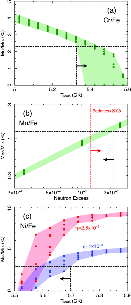
Figure 11.— (a) Relationship between $M_{\rm Cr}/M_{\rm Fe}$ and $T_{\rm peak}$ predicted by the delayed-detonation $M_{\rm Ch}$ SN Ia models presented in Yamaguchi et al. (2015). The horizontal and vertical dashed lines indicate the upper limit for the mass ratio observed in the Fe knot and the corresponding conservative lower limit for $T_{\rm peak}$, respectively. (b) Relationship between $M_{\rm Mn}/M_{\rm Fe}$ and $\eta$ expected for the burning cells with $5.3\times 10^{9}\lesssim T_{\rm peak}\,[{\rm K}]\lesssim 5.6\times 10^{9}$ of the same models as panel (a). The red vertical dashed line indicates the lower limit for $\eta$ determined by Badenes et al. (2008) for this SNR. (c) Relationship between $M_{\rm Ni}/M_{\rm Fe}$ and $T_{\rm peak}$ from the same models with different $\eta$ values of $1\times 10^{-3}$ (blue) and $2.5\times 10^{-3}$ (red). The observed mass ratio gives the upper limit for $T_{\rm peak}$ indicated by the vertical dashed line.

In order to constrain the burning regime that might have produced the Fe knot, we investigate grids of the standard delayed-detonation SN Ia models presented in Bravo & Martínez-Pinedo (2012) and Yamaguchi et al. (2015). The progenitor is assumed to be a $M_{\rm Ch}$ C+O white dwarf (suggested by previous work) with identical mass fractions of C and O. Figure 11(a) shows the predicted Cr/Fe mass ratio as a function of $T_{\rm peak}$, derived from relevant grids of these models. Although the values are calculated using a one-dimensional code (Bravo & Martínez-Pinedo 2012), the ranges of $\rho_{\rm peak}$ and neutron excess ($\eta$ $\equiv$ $1-2\left<Z_{A}/A\right>$, where $Z_{A}$ and $A$ are the atomic number and mass number, respectively) are reasonably covered. The excess neutrons are assumed to all come from ²²Ne (i.e., the metallicity effect: Timmes et al. 2003), and hence the neutronization due to the pre-explosion carbon simmering is neglected (Piro & Bildsten 2008; Martínez-Rodríguez et al. 2016). We find that the Cr yield is almost independent of $\eta$, and the Cr/Fe ratio monotonically decreases as $T_{\rm peak}$ increases. The observed upper limit is consistent with the models only when $T_{\rm peak}\gtrsim 5.3\times 10^{9}$ K.

The Mn yield from incomplete Si burning strongly depends on $\eta$, in addition to $T_{\rm peak}$ (Badenes et al. 2008). We thus investigate in Figure 11(b) the relationship between $M_{\rm Mn}/M_{\rm Fe}$ and $\eta$, predicted for the $T_{\rm peak}$ range constrained by the inferred Cr/Fe mass ratio. We find that the inferred $M_{\rm Mn}/M_{\rm Fe}$ upper limit requires $\eta\lesssim 2\times 10^{-3}$. On the other hand, Badenes et al. (2008) determined its lower limit to be $\sim$ $1.2\times 10^{-3}$, using the Mn/Cr mass ratio derived from the integrated ejecta spectrum. Our result does not conflict with theirs. If the effect of carbon simmering is negligible, then the relationship between $\eta$ and the progenitor’s metallicity $Z$ is given as $\eta$ = $0.101\times Z$ (Timmes et al. 2003). Therefore, the combined constraint from Badenes et al. (2008) and this work can be converted to $Z/Z_{\odot}$ = 0.9–1.5, using the up-to-date solar metallicity of $Z_{\odot}$ = 0.014 (Asplund et al. 2009). This combination should be valid as long as the progenitor purely consists of C, O, and ²²Ne, since the elemental composition (or $\eta$) in a $M_{\rm Ch}$ C+O white dwarf is naturally expected to be uniform (e.g., Iwamoto et al. 1999).

Finally, in Figure 11(c) we plot the relationship among $M_{\rm Ni}/M_{\rm Fe}$, $T_{\rm peak}$, and $\eta$, in the $\alpha$-NSE burning regime using the same nucleosynthesis models. For the low $\eta$ case (blue), the predicted $M_{\rm Ni}/M_{\rm Fe}$ ratio range matches the observed upper limit at $T_{\rm peak}\lesssim 5.7\times 10^{9}$ K. The high $\eta$ case (red) requires an even lower temperature of $<5.6\times 10^{9}$ K. In this temperature range, however, the predicted Mn/Fe ratio exceeds the inferred upper limit, unless $\eta\lesssim 2\times 10^{-3}$ (Figure 11(b)). Therefore, the high $\eta$ case is rejected also from the Ni/Fe mass ratio.

To summarize, Tycho’s Fe knot must have originated from either Si burning or $\alpha$-NSE regimes, probably close to their boundary with $T_{\rm peak}$ $\approx$ (5.3–5.7) $\times 10^{9}$ K, if the $M_{\rm Ch}$ C+O progenitor scenario is the case. The neutron excess in the pre-explosion white dwarf is accordingly constrained to be (1.2–2.0) $\times$ $10^{-3}$, which corresponds to the metallicity very close to the solar value. The normal freeze-out and n-NSE regimes are completely ruled out, indicating that the Fe knot does not come from near the core of a $M_{\rm Ch}$ white dwarf.

3.2. Comparison with a Multi-Dimensional Model

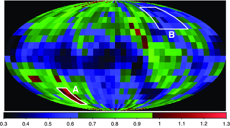
Figure 12.— $\left<R_{\rm Fe}\right>$/$\left<R_{\rm Si}\right>$ for each small cell in the spherical coordinate system predicted by the N100 model of Seitenzahl et al. (2013b). $\left<R_{\rm Fe}\right>$ and $\left<R_{\rm Si}\right>$ are defined as average radii of tracer particles with $5.3\leq T_{\rm peak}\,[{\rm GK}]\leq 5.7$ and $4.2\leq T_{\rm peak}\,[{\rm GK}]\leq 4.6$, respectively.

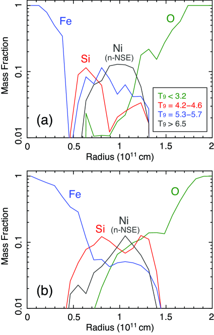
Figure 13.— Radial profiles of tracer particles that have experienced peak temperatures given in the legend (in the unit of GK) for the Fe prominence region (a: Region A in Figure 12) and the nearly-opposite side (b: Region B) at $t$ = 100 s. The dominant element for each curve is also indicated in the panels.

The next question is what mechanism created the Fe-rich clump and causes it to be observed now as a protrusion at the edge of the main SNR shell. One scenario is that the clump formed deep in the progenitor with sufficient density to not decelerate during the SNR evolution, and eventually broke out from the SNR surface (Wang & Chevalier 2002; Miceli et al. 2013; Tsebrenko & Soker 2015). Another possibility is that the Fe clump rose buoyantly during the SN explosion due to some instability (i.e., the Fe knot has been in the outer layer since the beginning of the remnant phase). As a first step to assess these possibilities, we investigate whether a modern multi-dimensional SN Ia model naturally predicts a small-scale Fe prominence overrunning the bulk of the IMEs. We choose the N100 model of Seitenzahl et al. (2013b) for this purpose, since it represents a typical SN Ia with a normal brightness, comparable with the inferred properties of Tycho’s progenitor (Badenes et al. 2006; Krause et al. 2008). We extract from the model the three-dimensional position of each tracer particle ($10^{6}$ particles in total) at $t$ = 100 s after the initial deflagration ignition and the peak temperature $T_{\rm peak}$ that each particle experienced (see Figure 4 of Seitenzahl et al. (2013b), for a guide). At this stage ($t$ = 100 s), the SN ejecta are almost freely expanding, and non-radial velocity components are negligible. Therefore, an outer particle should have a higher radial velocity. We define $\left<R_{\rm Fe}(\theta,\phi)\right>$ as an average radius of the particles with $5.3\leq T_{\rm peak}\,[{\rm GK}]\leq 5.7$ (the range constrained for the Tycho’s Fe knot) at a certain direction $(\theta,\phi)$. Similarly, $\left<R_{\rm Si}(\theta,\phi)\right>$ is defined as an average radius of the particles with $4.2\leq T_{\rm peak}\,[{\rm GK}]\leq 4.6$, where Si is synthesized most efficiently. Figure 12 shows the $\left<R_{\rm Fe}\right>$/$\left<R_{\rm Si}\right>$ distribution in the spherical coordinate system. We find a small region where the $\left<R_{\rm Fe}\right>$/$\left<R_{\rm Si}\right>$ value exceeds unity (Region A). Interestingly, its angular scale ($\sim$ 0.1$\pi$) is comparable with that of the Tycho Fe knot. Virtually everywhere else, $\left<R_{\rm Fe}\right>$/$\left<R_{\rm Si}\right>$ $<$ 1, consistent with the observed characteristic of Tycho’s SNR.

Figure 13(a) shows the radial distribution of the tracer particles at the Fe prominence region (Region A in Figure 12) from different burning regimes. For comparison, we show in Figure 13(b) the same distribution at the nearly opposite side of the SN (Region B). The presence of Fe ejecta outside the Si shell is confirmed in Region A, whereas a clear layered structure is formed in the other region similarly to Tycho’s NW rim. In short, the state-of-the-art numerical model of delayed-detonation SNe Ia qualitatively reproduces the inferred Fe distribution in Tycho’s SNR. However, the model also predicts a relatively large radius of n-NSE burning products (predominantly Mn and Ni) in both regions; this is not observationally confirmed, at least in the Fe knot. Such buoyant plumes of n-NSE products are expected as a consequence of a spherically-asymmetric deflagration (Seitenzahl et al. 2013b). In this sense, the lumpy morphology found in the Suzaku Ni K$\alpha$ image (Figure 2(c)) is intriguing—if real, this would be a clear signature of deflagration. Future study with more sensitive observations is encouraged.

3.3. Helium Detonation?

A possible alternative for the origin of the Fe knot is explosive He burning, which is thought to occur during an explosion of a sub-$M_{\rm Ch}$ white dwarf with a He mantle surrounding a C+O core (e.g., Woosley & Weaver 1994; Woosley & Kasen 2011). In this scenario, the first detonation ignites close to the bottom of the He mantle, which triggers the second detonation at the center of the white dwarf. The detonation in the He-rich environment can produce almost pure ⁵⁶Ni with some unburned $\alpha$-elements (e.g., Fink et al. 2007), naturally explaining the composition of the Fe knot; Knot B would then be interpreted as unburned material (see §2.5 and §2.6). However, the sub-$M_{\rm Ch}$ He detonation models tend to predict a sub-luminous SN Ia (Fink et al. 2007; Woosley & Kasen 2011), which is not the case for Tycho’s SNR (Ruiz-Lapuente 2004; Badenes et al. 2006; Krause et al. 2008). Moreover, this explosion scenario results in the production of a substantial amount of ⁵⁶Ni throughout the outer layers, not just one direction like in Tycho’s Fe knot (e.g., Moll & Woosley 2013). The He burning also leaves behind a large amount of unburnt $\alpha$ particles, and this would produce a substantial thermal continuum from bremsstrahlung that is not observed in this SNR. At this time, we cannot find any theoretical model that can perfectly reproduce all the observed characteristics of this SNR. If a very localized external detonation (in either pure He or C+O after Gyr-long gravitational deposition of ²²Ne) is allowed, both composition and location of the Fe knot may be explained.

Finally, we remark that the presence of Fe-rich material in the outer layer is not unique to this SNR. A similar Fe prominence is found in the young SN Ia remnant G1.9+0.3 (Borkowski et al. 2013). Fast-moving ⁵⁶Ni ejecta are also observed in the early phase of some SNe Ia, like SN 2010jn (Hachinger et al. 2013) and SN2014J (Diehl et al. 2014; Isern et al. 2016). These observations strongly imply that the creation of Fe-rich knots is a common occurrence in SNe Ia, and may play an important role in the explosion mechanism itself.

4. Conclusions

Taking advantage of the capabilities of Suzaku and Chandra, we have performed a detailed spatial and spectral study of the well-known Fe-rich knot in the east region of Tycho’s SNR. We have shown that the ionization timescale of this knot is clearly different from that of its Si-rich surroundings and the rest of the Fe ejecta, identifying it as a thermodynamically and chemically distinct structure within the SN ejecta. The absence of line emission from Mn and Ni implies that the knot did not originate in the deepest dense layers of a $M_{\rm Ch}$ SN progenitor affected by electron capture or normal freeze-out NSE burning, but was instead synthesized under incomplete Si burning or $\alpha$-rich freeze out with a relatively low neutron excess. Although the composition of the Fe knot could also be the result of explosive He burning, this hypothesis may require a very localized external detonation; otherwise a typical He-detonation scenario is in conflict with the main properties of the SNR and the spectroscopy of the light echo from SN 1572. During the explosion, the Fe knot somehow detached from the rest of the Fe-rich material, and formed a protrusion at the edge of the SN ejecta, beyond most of the Si-rich material. We estimate a total mass for the Fe knot of $\sim$ $7\times 10^{-3}$$M_{\odot}$, subject to considerable uncertainty. The physical process responsible for the formation of the knot is unclear at this time, but its spatial coincidence with a previously noted break in the reverse shock traced by hot Fe-rich material implies that it might have played a role in the explosion mechanism itself. Whatever its origin is, its presence in the best observed among a handful of Type Ia SNRs with spatially resolved X-ray spectroscopy strongly suggests that this kind of structure might be relatively common in SNe Ia.

References

- Arnaud (1996) Arnaud, K. A. 1996, in Astronomical Society of the Pacific Conference Series, Vol. 101, Astronomical Data Analysis Software and Systems V, ed. G. H. Jacoby & J. Barnes, 17
- Asplund et al. (2009) Asplund, M., Grevesse, N., Sauval, A. J., & Scott, P. 2009, ARA&A, 47, 481
- Badenes et al. (2006) Badenes, C., Borkowski, K. J., Hughes, J. P., Hwang, U., & Bravo, E. 2006, ApJ, 645, 1373
- Badenes et al. (2003) Badenes, C., Bravo, E., Borkowski, K. J., & Domínguez, I. 2003, ApJ, 593, 358
- Badenes et al. (2008) Badenes, C., Bravo, E., & Hughes, J. P. 2008, ApJ, 680, L33
- Badenes et al. (2007) Badenes, C., Hughes, J. P., Bravo, E., & Langer, N. 2007, ApJ, 662, 472
- Borkowski et al. (2013) Borkowski, K. J., Reynolds, S. P., Hwang, U., et al. 2013, ApJ, 771, L9
- Bravo & Martínez-Pinedo (2012) Bravo, E., & Martínez-Pinedo, G. 2012, Phys. Rev. C, 85, 055805
- Cassam-Chenaï et al. (2007) Cassam-Chenaï, G., Hughes, J. P., Ballet, J., & Decourchelle, A. 2007, ApJ, 665, 315
- Decourchelle et al. (2001) Decourchelle, A., Sauvageot, J. L., Audard, M., et al. 2001, A&A, 365, L218
- Diehl et al. (2014) Diehl, R., Siegert, T., Hillebrandt, W., et al. 2014, Science, 345, 1162
- Eriksen et al. (2011) Eriksen, K. A., Hughes, J. P., Badenes, C., et al. 2011, ApJ, 728, L28
- Fink et al. (2007) Fink, M., Hillebrandt, W., & Röpke, F. K. 2007, A&A, 476, 1133
- Hachinger et al. (2013) Hachinger, S., Mazzali, P. A., Sullivan, M., et al. 2013, MNRAS, 429, 2228
- Hayato et al. (2010) Hayato, A., Yamaguchi, H., Tamagawa, T., et al. 2010, ApJ, 725, 894
- Hwang & Gotthelf (1997) Hwang, U., & Gotthelf, E. V. 1997, ApJ, 475, 665
- Hwang et al. (1998) Hwang, U., Hughes, J. P., & Petre, R. 1998, ApJ, 497, 833
- Hwang & Laming (2012) Hwang, U., & Laming, J. M. 2012, ApJ, 746, 130
- Isern et al. (2016) Isern, J., Jean, P., Bravo, E., et al. 2016, A&A, 588, A67
- Iwamoto et al. (1999) Iwamoto, K., Brachwitz, F., Nomoto, K., et al. 1999, ApJS, 125, 439
- Krause et al. (2008) Krause, O., Tanaka, M., Usuda, T., et al. 2008, Nature, 456, 617
- Maoz et al. (2014) Maoz, D., Mannucci, F., & Nelemans, G. 2014, ARA&A, 52, 107
- Martínez-Rodríguez et al. (2016) Martínez-Rodríguez, H., Piro, A. L., Schwab, J., & Badenes, C. 2016, ApJ, 825, 57
- Mazzali et al. (2007) Mazzali, P. A., Röpke, F. K., Benetti, S., & Hillebrandt, W. 2007, Science, 315, 825
- Miceli et al. (2013) Miceli, M., Orlando, S., Reale, F., Bocchino, F., & Peres, G. 2013, MNRAS, 430, 2864
- Miceli et al. (2015) Miceli, M., Sciortino, S., Troja, E., & Orlando, S. 2015, ApJ, 805, 120
- Moll & Woosley (2013) Moll, R., & Woosley, S. E. 2013, ApJ, 774, 137
- Ozawa et al. (2009) Ozawa, M., Uchiyama, H., Matsumoto, H., et al. 2009, PASJ, 61, 1
- Park et al. (2007) Park, S., Hughes, J. P., Slane, P. O., et al. 2007, ApJ, 670, L121
- Park et al. (2013) Park, S., Badenes, C., Mori, K., et al. 2013, ApJ, 767, L10
- Piro & Bildsten (2008) Piro, A. L., & Bildsten, L. 2008, ApJ, 673, 1009
- Ruiz-Lapuente (2004) Ruiz-Lapuente, P. 2004, ApJ, 612, 357
- Sato & Hughes (2016) Sato, T., & Hughes, J. P. 2016, ArXiv e-prints, arXiv:1605.09059
- Seitenzahl et al. (2013a) Seitenzahl, I. R., Cescutti, G., Röpke, F. K., Ruiter, A. J., & Pakmor, R. 2013a, A&A, 559, L5
- Seitenzahl et al. (2013b) Seitenzahl, I. R., Ciaraldi-Schoolmann, F., Röpke, F. K., et al. 2013b, MNRAS, 429, 1156
- Serlemitsos et al. (2007) Serlemitsos, P. J., Soong, Y., Chan, K.-W., et al. 2007, PASJ, 59, 9
- Tamagawa et al. (2009) Tamagawa, T., Hayato, A., Nakamura, S., et al. 2009, PASJ, 61, S167
- Tanaka et al. (2011) Tanaka, M., Mazzali, P. A., Stanishev, V., et al. 2011, MNRAS, 410, 1725
- Thielemann et al. (1986) Thielemann, F.-K., Nomoto, K., & Yokoi, K. 1986, A&A, 158, 17
- Tian & Leahy (2011) Tian, W. W., & Leahy, D. A. 2011, ApJ, 729, L15
- Timmes et al. (2003) Timmes, F. X., Brown, E. F., & Truran, J. W. 2003, ApJ, 590, L83
- Tsebrenko & Soker (2015) Tsebrenko, D., & Soker, N. 2015, MNRAS, 453, 166
- Vancura et al. (1995) Vancura, O., Gorenstein, P., & Hughes, J. P. 1995, ApJ, 441, 680
- Wang & Chevalier (2002) Wang, C.-Y., & Chevalier, R. A. 2002, ApJ, 574, 155
- Warren et al. (2005) Warren, J. S., Hughes, J. P., Badenes, C., et al. 2005, ApJ, 634, 376
- Williams et al. (2013) Williams, B. J., Borkowski, K. J., Ghavamian, P., et al. 2013, ApJ, 770, 129
- Wilms et al. (2000) Wilms, J., Allen, A., & McCray, R. 2000, ApJ, 542, 914
- Woosley & Kasen (2011) Woosley, S. E., & Kasen, D. 2011, ApJ, 734, 38
- Woosley & Weaver (1994) Woosley, S. E., & Weaver, T. A. 1994, ApJ, 423, 371
- Yamaguchi et al. (2008) Yamaguchi, H., Koyama, K., Katsuda, S., et al. 2008, PASJ, 60, S141
- Yamaguchi et al. (2014a) Yamaguchi, H., Badenes, C., Petre, R., et al. 2014a, ApJ, 785, L27
- Yamaguchi et al. (2014b) Yamaguchi, H., Eriksen, K. A., Badenes, C., et al. 2014b, ApJ, 780, 136
- Yamaguchi et al. (2015) Yamaguchi, H., Badenes, C., Foster, A. R., et al. 2015, ApJ, 801, L31
- Yang et al. (2013) Yang, X. J., Tsunemi, H., Lu, F. J., et al. 2013, ApJ, 766, 44
- Yasumi et al. (2014) Yasumi, M., Nobukawa, M., Nakashima, S., et al. 2014, PASJ, 66, 68