ModelHub: Lifecycle Management for Deep Learning

Towards a Unified Framework for Data and Lifecycle Management for Deep Learning

Unified Lifecycle Management for Deep Learning

Towards Unified Data and Lifecycle Management for Deep Learning

Abstract

Deep learning has improved state-of-the-art results in many important fields, and has been the subject of much research in recent years, leading to the development of several systems for facilitating deep learning. Current systems, however, mainly focus on model building and training phases, while the issues of data management, model sharing, and lifecycle management are largely ignored. Deep learning modeling lifecycle generates a rich set of data artifacts, such as learned parameters and training logs, and comprises of several frequently conducted tasks, e.g., to understand the model behaviors and to try out new models. Dealing with such artifacts and tasks is cumbersome and largely left to the users. This paper describes our vision and implementation of a data and lifecycle management system for deep learning. First, we generalize model exploration and model enumeration queries from commonly conducted tasks by deep learning modelers, and propose a high-level domain specific language (DSL), inspired by SQL, to raise the abstraction level and accelerate the modeling process. To manage the data artifacts, especially the large amount of checkpointed float parameters, we design a novel model versioning system (dlv), and a read-optimized parameter archival storage system (PAS) that minimizes storage footprint and accelerates query workloads without losing accuracy. PAS archives versioned models using deltas in a multi-resolution fashion by separately storing the less significant bits, and features a novel progressive query (inference) evaluation algorithm. Third, we show that archiving versioned models using deltas poses a new dataset versioning problem and we develop efficient algorithms for solving it. We conduct extensive experiments over several real datasets from computer vision domain to show the efficiency of the proposed techniques.

I Introduction

Deep learning models, also called deep neural networks (DNN), have dramatically improved the state-of-the-art results for many important reasoning and learning tasks including speech recognition, object recognition, and natural language processing in recent years [1]. Learned using massive amounts of training data, DNN models have superior generalization capabilities, and the intermediate layers in many deep learning models have been proven useful in providing effective semantic features that can be used with other learning techniques and are applicable to other problems. However, there are many critical large-scale data management issues in learning, storing, sharing, and using deep learning models, which are largely ignored by researchers today, but are coming to the forefront with the increased use of deep learning in a variety of domains. In this paper, we discuss some of those challenges in the context of the modeling lifecycle, and propose a comprehensive system to address them. Given the large scale of data involved (both training data and the learned models themselves) and the increasing need for high-level declarative abstractions, we argue that database researchers should play a much larger role in this area. Although this paper primarily focuses on deep neural networks, similar data management challenges are seen in lifecycle management of others types of ML models like logistic regression, matrix factorization, etc.

DNN Modeling Lifecycle and Challenges: Compared with the traditional approach of feature engineering followed by model training [2], deep learning is an end-to-end learning approach, i.e., the features are not given by a human but are learned in an automatic manner from the input data. Moreover, the features are complex and have a hierarchy along with the network representation. This requires less domain expertise and experience from the modeler, but understanding and explaining the learned models is difficult; why even well-studied models work so well is still a mystery and under active research. Thus, when developing new models, changing the learned model (especially its network structure and hyper-parameters) becomes an empirical search task.

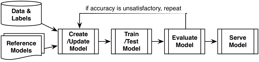
Figure 1: Deep Learning Modeling Lifecycle

In Fig. 1, we show a typical deep learning modeling lifecycle (we present an overview of deep neural networks in the next section). Given a prediction task, a modeler often starts from well-known models that have been successful in similar task domains; she then specifies input training data and output loss functions, and repeatedly adjusts the DNN on operators and connections like Lego bricks, tunes model hyper-parameters, trains and evaluates the model, and repeats this loop until prediction accuracy does not improve. Due to a lack of understanding about why models work, the adjustments and tuning inside the loop are driven by heuristics, e.g., adjusting hyper-parameters that appear to have a significant impact on the learned weights, applying novel layers or tricks seen in recent empirical studies, and so on. Thus, many similar models are trained and compared, and a series of model variants needs to be explored and developed. Due to the expensive learning/training phase, each iteration of the modeling loop takes a long period of time and produces many (checkpointed) snapshots of the model. As we noted above, this is a common workflow across many other ML models as well.

Current systems (Caffe [3], Theano, Torch, TensorFlow [4], etc.) mainly focus on model building and training phases, while the issues of data management, model sharing, and lifecycle management are largely ignored. Modelers are required to write external imperative scripts, edit configurations by hand and manually maintain a manifest of model variations that have been tried out; not only are these tasks irrelevant to the modeling objective, but they are also challenging and nontrivial due to the complexity of the model as well as large footprints of the learned models. More specifically, the tasks and data artifacts in the modeling lifecycle expose several systems and data management challenges, which include:

• Understanding & Comparing Models: It is difficult to keep track of the many models developed and/or understand the differences amongst them. Differences among both the metadata about the model (training sample, hyperparameters, network structure, etc.), as well as the actual learned parameters, are of interest. It is common to see a modeler write all configurations in a spreadsheet to keep track of temporary folders of input, setup scripts, snapshots and logs, which is not only a cumbersome but also an error-prone process.

• Repetitive Adjusting of Models: The development lifecycle itself has time-consuming repetitive sub-steps, such as adding a layer at different places to adjust a model, searching through a set of hyper-parameters for the different variations, reusing learned weights to train models, etc., which currently have to be performed manually.

• Model Versioning: Similar models are possibly trained and run multiple times, reusing others’ weights as initialization, either because of a changed input or discovery of an error. There is thus a need to keep track of multiple model versions and their relationships over time, although the utilities of different models are very different.

• Parameter Archiving: The storage footprint of deep learning models tends to be very large. Recent top-ranked models in the ImageNet task have billions of floating-point parameters and require hundreds of MBs to store one snapshot during training. Due to resource constraints, the modeler has to limit the number of snapshots, even drop all snapshots of a model at the cost of retraining when needed.

• Reasoning about Model Results: Another key data artifact that often needs to be reasoned about is the results of running a learned model on the training or testing dataset. By comparing the results across different models, a modeler can get insights into difficult training examples or understand correlations between specific adjustments and the performance.

In addition, although not a focus of this paper, sharing and reusing models is not easy, especially because of the large model sizes and specialized tools used for learning and modeler generated scripts in the lifecycle.

ModelHub: In this paper, we propose the ModelHub system to address these challenges. The ModelHub system is not meant to replace popular training-focused DNN systems, but rather designed to be used with them to accelerate modeling tasks and manage the rich set of lifecycle artifacts. It consists of three key components: (a) a model versioning system (DLV) to store, query and aid in understanding the models and their versions, (b) a model network adjustment and hyper-parameter tuning domain specific language (DQL) to serve as an abstraction layer to help modelers focus on the creation of the models, (c) a hosted deep learning model sharing system (ModelHub) to exchange DLV repositories and enable publishing, discovering and reusing models from others.

The key features and innovative design highlights of ModelHub are: (a) We use a git-like VCS interface as a familiar user interface to let the modeler manage and explore the created models in a repository, and an SQL-like model enumeration DSL to aid modelers in making and examining multiple model adjustments easily. (b) Behind the declarative constructs, ModelHub manages different artifacts in a split back-end storage: structured data, such as network structure, training logs of a model, lineages of different model versions, output results, are stored in a relational database, while learned float-point parameters of a model are viewed as a set of float matrices and managed in a read-optimized archival storage (PAS). (c) Parameters dominate the storage footprint and floats are well-known at being difficult to compress. We study PAS implementation thoroughly under the context of DNN query workload and advocate a segmented approach to store the learned parameters, where the low-order bytes are stored independently of the high-order bytes. We also develop novel model evaluation schemes to use high order bytes solely and progressively uncompress less-significant chunks if needed to ensure the correctness of an inference query. (d) Due to the different utility of developed models, archiving versioned models using parameter matrix deltas exhibits a new type of dataset versioning problem which not only optimizes between storage and access tradeoff but also has model-level constraints. (e) Finally, the VCS model repository design extends naturally to a collaborative format and online system which contain rich model lineages and enables sharing, reusing, reproducing DNN models which are compatible across training systems.

Contributions: Our key research contributions are:

• We propose the first comprehensive DNN lifecycle management system, study its design requirements, and propose declarative constructs (DLV and DQL) to provide high-level abstractions.

• We develop PAS, a read-optimized archival storage system for dealing with a large collection of versioned float matrices.

• We formulate a new dataset versioning problem with co-usage constraints, analyze its complexity, and design efficient algorithms for solving it.

• We develop a progressive, approximate query evaluation scheme that avoids reading low-order bytes of the parameter matrices unless necessary.

• We present a comprehensive evaluation of ModelHub that shows the proposed techniques are useful in real life models, and scale well on synthetic models.

Outline: In Section II, we provide background on related topics in DNN modeling lifecycle. In Section III, we present an overview of ModelHub, and discuss the declarative interfaces. We describe the parameter archival store (PAS) in Section IV, present an experimental evaluation in Section V, and closely related work in Section VI.

Figure 2: Anatomy of A DNN Model (LeNet)

II Background

To support our design decisions, we overview the artifacts and common task practices in DNN modeling lifecycle.

Deep Neural Networks: A deep learning model is a deep neural network (DNN) consisting of many layers having nonlinear activation functions that are capable of representing complex transformations between input data and desired output. Let $\mathbb{D}$ denote a data domain and $\mathbb{O}$ denote a prediction label domain (e.g., $\mathbb{D}$ may be a set of images; $\mathbb{O}$ may be the names of the set of objects we wish to recognize, i.e, labels). As with any prediction model, a DNN is a mapping function $f:\mathbb{D}\to\mathbb{O}$ that minimizes a certain loss function $L$, and is of the following form:

Here $i$ denotes the layer number, $(W_{i},b_{i})$ are learnable weights and bias parameters in layer $i$, and $\sigma_{i}$ is an activation function that non-linearly transforms the result of the previous layer (common activation functions include sigmoid, ReLU, etc.). Given a learned model and an input $d$, applying $f_{0},f_{1},...,f_{n}$ in order gives us the prediction label for that input data. In the training phase, the model parameters are learned by minimizing $L(f_{n},l_{d})$, typically done through iterative methods, such as stochastic gradient descent.

Fig. 2 shows a classic convolutional DNN, LeNet. LeNet is proposed to solve a prediction task from handwritten images to digit labels $\{0\cdots 9\}$. In the figure, a cube represents an intermediate tensor, while the dotted lines are unit transformations between tensors. More formally, a layer, $L_{i}:(W,H,X)\mapsto Y$, is a function which defines data transformations from tensor $X$ to tensor $Y$. $W$ are the parameters which are learned from the data, and $H$ are the hyperparameters which are given beforehand. A layer is non-parametric if $W=\emptyset$.

In the computer vision community, the layers defining transformations are considered building blocks of a DNN model, and referred to using a conventional name, such as full layer, convolution layer, pool layer, normalization layer, etc. The chain is often called the network architecture. The LeNet architecture has two convolution layers, each followed by a pool layer, and two full layers, shown with layer shapes and hyperparameters in Fig. 2. Moreover, winning models in recent ILSVRC (ImageNet Large Scale Vision Recognition Competitions) are shown in Table I, with their architectures described by a composition of common layers in regular expressions syntax for illustrating the similarities (Note the activation functions and detailed connections are omitted).

DNN models are learned from massive data based on some architecture, and modern successful computer vision DNN architectures consist of a large number of float weight parameters (flops) shown in Table I, resulting in large storage footprints (GBs) and long training times (often weeks). Furthermore, the training process is often checkpointed and variations of models need to be explored, leading to many model copies.

Modeling Data Artifacts: Unlike many other prediction methods, DNN modeling results in a very large number of weight parameters, a rich set of hyperparameters, and learning measurements, which are used in unique ways in practice, resulting in a mixture of structured data, files and binary floating number artifacts:

• Non-convexity & Hyperparameters: A DNN model is typically non-convex, and $\{W\}$ is a local optimum of the underlying loss-minimization problem. Optimization procedure employs many tricks to reach a solution quickly [5]. The set of hyperparameters (e.g., learning rate, momentum) w.r.t. to the optimization algorithm need to be maintained.

• Iterations & Measurements: Models are trained iteratively and checkpointed periodically due to the long running times. A set of learning measurements are collected in various logs, including objective loss values and accuracy scores.

• Fine-tuning & Snapshots: Well-known models are often learned from massive real-world data (ImageNet), and require large amounts of resources to train; when prediction tasks do not vary much (e.g., animal recognition vs dog recognition), the model parameters are reused as initializations and adjusted using new data; this is often referred to as fine-tuning. On the other hand, not all snapshots can be simply deleted, as the convergence is not monotonic.

• Provenance & Arbitrary Files: Alternate ways to construct architectures or to set hyperparameters lead to human-in-the-loop model adjustments. Initialization, preprocessing schemes, and hand-crafted scripts are crucial provenance information to explore models and reproduce results.

Network	Architecture (in regular expression)	$|W|$ (flops)
LeNet [6]	$(L_{conv}L_{pool})\{2\}L_{ip}\{2\}$	$4.31\times 10^{5}$
AlexNet [7]	$(L_{conv}L_{pool})\{2\}(L_{conv}\{2\}L_{pool})\{2\}L_{ip}\{3\}$	$6\times 10^{7}$
VGG [8]	$(L_{conv}\{2\}L_{pool})\{2\}(L_{conv}\{4\}L_{pool})\{3\}L_{ip}\{3\}$	$1.96\times 10^{10}$
ResNet [9]	$(L_{conv}L_{pool})(L_{conv})\{150\}L_{pool}L_{ip}$	$1.13\times 10^{10}$

TABLE I: Popular CNN Models for Object Recognition

Model Adjustment: In a modeling lifecycle for a prediction task, the update-train-evaluate loop is repeated in daily work, and many model variations are adjusted and trained. In general, once data and loss are determined, model adjustment can be done in two orthogonal steps: a) network architecture adjustments where layers are dropped or added and layer function templates are varied, and b) hyperparameter selections, which affect the behavior of the optimization algorithms. There is much work on search strategies to enumerate and explore both.

Model Sharing: Due to the good generalizability, long training times, and verbose hyperparameters required for large DNN models, there is a need to share the trained models. Jia et al. [3] built an online venue (Caffe Model Zoo) to share models. Briefly, Model Zoo is part of a github repository with a markdown file edited collaboratively. To publish models, modelers add an entry with links to download trained parameters in caffe format. Apart from the caffe community, similar initiatives are in place for other training systems.

III ModelHub System Overview

We show the ModelHub architecture including the key components and their interactions in Fig. 3. At a high level, the ModelHub functionality is divided among a local component and a remote component. The local functionality includes the integration with popular DNN systems such as caffe, torch, tensorflow, etc., on a local machine or a cluster. The remote functionality includes sharing of models, and their versions, among different groups of users. We primarily focus on the local functionality in this paper.

On the local system side, DLV is a version control system (VCS) implemented as a command-line tool (dlv), that serves as an interface to interact with the rest of the local and remote components. Use of a specialized VCS instead of a general-purpose VCS such as git or svn allows us to better portray and query the internal structure of the artifacts generated in a modeling lifecycle, such as network definitions, training logs, binary weights, and relationships between models. The key utilities of dlv are listed in Table II, grouped by their purpose; we explain these in further detail in Sec. III-B. DQL is a DSL we propose to assist modelers in deriving new models; the DQL query parser and optimizer components in the figure are used to support this language. The model learning module interacts with external deep learning tools that the modeler uses for training and testing. They are essentially wrappers on specific DNN systems that extract and reproduce modeling artifacts. Finally, the ModelHub service is a hosted toolkit to support publishing, discovering and reusing models, and serves similar role for DNN models as github for software development or DataHub for data science [10].

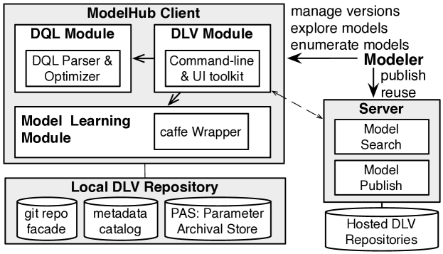
Figure 3: ModelHub System Architecture

III-A Data Model

ModelHub works with two data models: a conceptual DNN model, and a data model for the versions in a DLV repository.

DNN Model: A DNN model can be understood in different ways, as one can tell from the different model creation APIs in popular deep learning systems. In the formulation mentioned in Sec. I, if we view a function $f_{i}$ as a node and dependency relationship $(f_{i},f_{i-1})$ as an edge, it becomes a directed acyclic graph (DAG). Depending on the granularity of the function in the DAG, either at the tensor arithmetic operator level (add, multiply), or at a logical composition of those operators (convolution layer, full layer), it forms different types of DAGs. In ModelHub, we consider a DNN model node as a composition of unit operators (layers), often adopted by computer vision models. The main reason for this decision is that we focus on productivity improvement in the lifecycle, rather than implementation efficiencies of training and testing.

VCS Data Model: When managing DNN models in the VCS repository, a model version represents the contents in a single version. It consists of a network definition, a collection of weights (each of which is a value assignment for the weight parameters), a set of extracted metadata (such as hyper-parameter, accuracy and loss generated in the training phase), and a collection of files used together with the model instance (e.g., scripts, datasets). In addition, we enforce that a model version must be associated with a human readable name for better utility, which reflects the logical groups of a series of improvement efforts over a DNN model in practice.

In the implementation, model versions can be viewed as a relation model_version$($name, id, N, W, M, F$)$, where id is part of the primary key of model versions and is auto-generated to distinguish model versions with the same name. In brief, $N,W,M,F$ are the network definition, weight values, extracted metadata and associated files respectively. The DAG, N, is stored as two tables: Node$($id, node, A$)$, where $A$ is a list of attributes such as layer name, and Edge$($from, to$)$. $W$ is managed in our learned parameter storage (PAS, Sec. IV). $M$, the metadata, captures the provenance information of training and testing a particular model; it is extracted from training logs by the wrapper module, and includes the hyperparameters when training a model, the loss and accuracy measures at some iterations, as well as dynamic parameters in the optimization process, such as learning rate at some iterations. Finally, $F$ is file list marked to be associated with a model version, including data files, scripts, initial configurations, and etc. Besides a set of model versions, the lineage of the model versions are captured using a separate parent$($base, derived, commit$)$ relation. All of these relations are maintained/updated in a relational backend when the modeler runs the different dlv commands that update the repository.

Type	Command	Description
model version management	init	Initialize a dlv repository.
	add	Add model files to be committed.
	commit	Commit the added files.
	copy	Scaffold model from an old one.
	archive	Archive models in the repository.
model exploration	list	List models and related lineages.
	desc	Describe a particular model.
	diff	Compare multiple models.
	eval	Evaluate a model with given data.
model enumeration	query	Run DQL clause.
remote interaction	publish	Publish a model to ModelHub.
	search	Search models in ModelHub.
	pull	Download from ModelHub.

TABLE II: A list of key dlv utilities.

III-B Query Facilities

Once the DNN models and their relationships are managed in DLV, the modeler can interact with them easily. The query facilities we provide can be categorized into two types: a) model exploration queries and b) model enumeration queries.

III-B1 Model Exploration Queries

Model exploration queries interact with the models in a repository, and are used to understand a particular model, to query lineages of the models, and to compare several models. For usability, we design it as query templates via dlv sub-command, similar to other VCS.

List Models & Related Lineages: By default, the query lists all versions of all models including their commit descriptions and parent versions; it also takes options, such as showing results for a particular model, or limiting the number of versions to be listed.
dlv list [--model_name] [--commit_msg] [--last]

Describe Model: dlv desc shows the extracted metadata from a model version, such as the network definition, learnable parameters, execution footprint (memory and runtime), activations of convolutional DNNs, weight matrices, and evaluation results across iterations. Note the activation is the intermediate output of a DNN model in computer vision and often used as an important tool to understand the model. The current output formats are a result of discussions with computer vision modelers to deliver tools that fit their needs. In addition to printing to console, the query supports HTML output for displaying the images and visualizing the weight distribution.
dlv desc [--model_name $|$ --version] [--output]

Compare Models: dlv diff takes a list of model names or version ids and allows the modeler to compare the DNN models. Most of desc components are aligned and returned in the query result side by side.
dlv diff [--model_names $|$ --versions] [--output]

Evaluate Model: dlv eval runs test phase of the managed models with an optional config specifying different data or changes in the current hyper-parameters. The main usages of exploration query are two-fold: 1) for the users to get familiar with a new model, 2) for the user to test known models on different data or settings. The query returns the accuracy and optionally the activations. It is worth pointing out that complex evaluations can be done via model enumeration queries in DQL.
dlv eval [--model_name $|$ --versions] [--config]

III-B2 Model Enumeration Queries

Model enumeration queries are used to explore variations of currently available models in a repository by changing network structures or tuning hyper-parameters. There are several operations that need to be done in order to derive new models: 1) Select models from the repository to improve; 2) Slice particular models to get reusable components; 3) Construct new models by mutating the existing ones; 4) Try the new models on different hyper-parameters and pick good ones to save and work with. When enumerating models, we also want to stop exploration of bad models early.

To support this rich set of requirements, we propose the DQL domain specific language, that can be executed using “dlv query”. Challenges of designing the language are: a) the data model is a mix of relational and the graph data models and b) the enumeration includes hyper-parameter tuning as well as network structure mutations, which are very different operations. We omit a thorough explanation of the language due to space constraints, and instead show the key operators and constructs along with a set of examples (Query 1$\sim$4) to show how requirements are met.

⬇

select m1

where m1.name like "alexnet_%" and

m1.creation_time > "2015-11-22" and

m1["conv[1,3,5]"].next has POOL("MAX")

Query 1: DQL select query to pick the models.           

⬇

slice m2 from m1

where m1.name like "alexnet-origin%"

mutate m2.input = m1["conv1"] and

m2.output = m1["fc7"]

Query 2: DQL slice query to get a sub-network.          

⬇

construct m2 from m1

where m1.name like "alexnet-avgv1%" and

m1["conv*($1)"].next has POOL("AVG")

mutate m1["conv*($1)"].insert = RELU("relu$1")

Query 3: DQL construct query to derive more models on existing ones. 

⬇

evaluate m

from "query3"

with config = "path to config"

vary config.base_lr in [0.1, 0.01, 0.001] and

config.net["conv*"].lr auto and

config.input_data in ["path1", "path2"]

keep top(5, m["loss"], 100)

Query 4: DQL evaluate query to enumerate models with different network architectures, search hyper-parameters, and eliminate models.

Key Operators: We adopt the standard SQL syntax to interact with the repository. DQL views the repository as a single model version table. A model version instance is a DAG, which can be viewed as object types in modern SQL conventions. In DQL, attributes can be referenced using attribute names (e.g. m1.name, m1.creation_time, m2.input, m2.output), while navigating the internal structures of the DAG, i.e. the Node and Edge EDB, we provide a regexp style selector operator on a model version to access individual DNN nodes, e.g. m1["conv[1,3,5]"] in Query 1 filters the nodes in m1. Once the selector operator returns a set of nodes, prev and next attributes of the node allow 1-hop traversal in the DAG. Note that POOL("MAX") is one of the standard built-in node templates for condition clauses. Using SPJ operators with object type attribute access and the selector operator, we allow relational queries to be mixed with graph traversal conditions.

To retrieve reusable components in a DAG, and mutate it to get new models, we provide slice, construct and mutate operators. Slice originates in programming analysis research; given a start and an end node, it returns a subgraph including all paths from the start to the end and the connections which are needed to produce the output. Construct can be found in graph query languages such as SPARQL to create new graphs. We allow construct to derive new DAGs by using selected nodes to insert nodes by splitting an outgoing edge or to delete an outgoing edge connecting to another node. Mutate limits the places where insert and delete can occur. For example, Query 2 and 3 generate reusable subgraphs and new graphs. Query 2 slices a sub-network from matching models between convolution layer ‘conv1’ and full layer ‘fc7’, while Query 3 derives new models by appending a ReLU layer after all convolution layers followed by an average pool. All queries can be nested.

Finally, evaluate can be used to try out new models, with potential for early out if expectations are not reached. We separate the network enumeration component from the hyper-parameter turning component; while network enumeration can be nested in the from clause, we introduce a with operator to take an instance of a tuning config template, and a vary operator to express the combination of activated multi-dimensional hyper-parameters and search strategies. auto is keyword implemented using default search strategies (currently grid search). To stop early and let the user control the stopping logic, we introduce a keep operator to take a rule consisting of stopping condition templates, such as top-k of the evaluated models, or accuracy threshold. Query 4 evaluates the models constructed and tries combinations of at least three different hyper-parameters, and keeps the top 5 models w.r.t. the loss after 100 iterations.

III-C ModelHub Implementation

On the local side, the current implementation of ModelHub maintains the data model in multiple back-ends and utilizes git to manage the arbitrary file diffs. Various queries are decomposed and sent to different backends and chained accordingly. On the other hand, as the model repository is standalone, we host the repositories as a whole in a ModelHub service. The modeler can use the dlv publish to push the repository for archiving, collaborating or sharing, and use dlv search and dlv pull to discover and reuse remote models. We envision such a form of collaboration can facilitate a learning environment, as all versions in the lifecycle are accessible and understandable with ease.

IV Parameter archival storage (PAS)

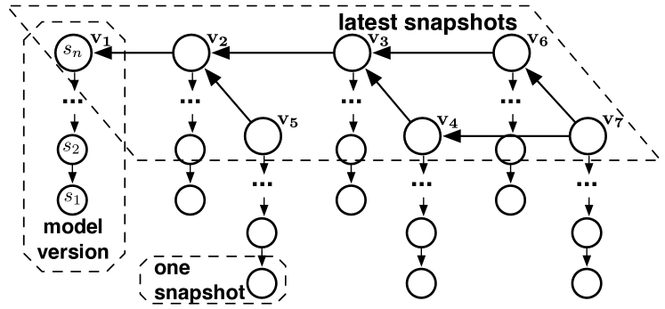
Figure 4: Relationships of Model Versions and Snapshots

Modeling lifecycle for DNNs, and machine learning models in general, is centered around the learned parameters, whose storage footprint can be very large. The goal of PAS is to maintain a large number of learned models as compactly as possible, without compromising on the query performance. Before introducing our design, we first discuss the queries of interest, and some key properties of the model artifacts. We then describe different options to store a single float matrix, and to construct deltas (differences) between two matrices. We then formulate the optimal version graph storage problem, discuss how it differs from the prior work, and present algorithms for solving it. Finally, we develop a novel approximate model evaluation technique, suitable for the segmented storage technique that PAS uses.

IV-A Weight Parameters & Query Type of Interests

We illustrate the key weight parameter artifacts and the relationships among them in Fig. 4, and also explain some of the notations used in this section. At a high level, the predecessor-successor relationships between all the developed models is captured as a version graph. These relationships are user-specified and conceptual in nature, and the interpretation is left to the user (i.e., an edge $v_{i}\rightarrow v_{j}$ indicates that $v_{j}$ was an updated version of the model that the user checked in after $v_{i}$, but the nature of this update is irrelevant for storage purposes). A model version $v_{i}$ itself consists of a series of snapshots, $s_{1},...,s_{n}$, which represent checkpoints during the training process (most systems will take such snapshots due to the long running times of the iterations). We refer the last or the best checkpointed snapshot $s_{n}$ as the latest snapshot of $v_{i}$, and denote it by $s_{v_{i}}$.

One snapshot, in turn, consists of intermediate data $X$ and trained parameters $W$ (e.g., in Fig. 2, the model has $431080$ parameters for $W$, and $19694\cdot b$ dimensions for $X$, where $b$ is the minibatch size). Since $X$ is useful only if training needs to be resumed, only $W$ is stored in PAS. Outside of a few rare exceptions, $W$ can always be viewed as a collection of float matrices, $\mathbb{R}^{m\times n},m\geq 1,n\geq 1$, which encode the weights on the edges from outputs of the neurons in one layer to the inputs of the neurons in the next layer. Thus, we treat a float matrix as a first class data type in PAS.

The retrieval queries of interest are dictated by the operations that are done on these stored models, which include: (a) testing a model, (b) reusing weights to fine-tune other models, (c) comparing parameters of different models, (d) comparing the results of different models on a dataset, and (e) model exploration queries (Sec. III-B). Most of these operations require execution of group retrieval queries, where all the weight matrices in a specific snapshot need to be retrieved. This is different from range queries seen in array databases (e.g., SciDB), and also have unique characteristics that influence the storage and retrieval algorithms.

• Similarity among Fine-tuned Models: Although non-convexity of the training algorithm and differences in network architectures across models lead to non-correlated parameters, the widely-used fine-tuning practices (Sec. II) generate model versions with similar parameters, resulting in efficient delta encoding schemes.

• Co-usage constraints: Prior work on versioning and retrieval [11] has focused on retrieving a single artifact stored in its entirety. However, we would like to store the different matrices in a snapshot independently of each other, but we must retrieve them together. These co-usage constraints make the prior algorithms inapplicable as we discuss later.

• Low Precision Tolerance: DNNs are well-known for their tolerance to using low-precision floating point numbers (Sec. VI), both during training and evaluation. Further, many types of queries (e.g., visualization and comparisons) do not require retrieving the full-precision weights.

• Unbalanced Access Frequencies: Not all snapshots are used frequently. The latest snapshots with the best testing accuracy are used in most of the cases. The checkpointed snapshots have limited usages, including debugging and comparisons.

IV-B Parameters As Segmented Float Matrices

Float Data Type Schemes: Although binary (1/-1) or ternary (1/0/-1) matrices are sometimes used in DNNs, in general PAS handles real number weights. Due to different usages of snapshots, PAS offers a handful of float representations to let the user trade-off storage efficiency with lossyness using dlv.

• Float Point: DNNs are typically trained with single precision (32 bit) floats. This scheme uses the standard IEEE 754 floating point encoding to store the weights with sign, exponent, and mantissa bits. IEEE half-precision proposal (16 bits) and tensorflow truncated 16bits [4] are supported as well and can be used if desired.

• Fixed Point: Fixed point encoding has a global exponent per matrix, and each float number only has sign and mantissa using all $k$ bits. This scheme is a lossy scheme as tail positions are dropped, and a maximum of $2^{k}$ different values can be expressed. The entropy of the matrix also drops considerably, aiding in compression.

• Quantization: Similarly, PAS supports quantization using $k$ bits, $k\leq 8$, where $2^{k}$ possible values are allowed. The quantization can be done in random manner or uniform manner by analyzing the distribution, and a coding table is used to maintain the integer codes stored in the matrices in PAS. This is most useful for snapshots whose weights are primarily used for fine-tuning or initialization.

The float point schemes present here are not new, and are used in DNN systems in practice [12, 13, 14]. As a lifecycle management tool, PAS lets experienced users select schemes rather than deleting snapshots due to resource constraints. Our evaluation shows storage/accuracy tradeoffs of these schemes.

Bytewise Segmentation for Float Matrices: One challenge for PAS is the high entropy of float numbers in the float arithmetic representations, which leads to them being very hard to compress. Compression ratio shown in related work for scientific float point datasets, e.g., simulations, is very low. The state of art compression schemes do not work well for DNN parameters either (Sec. VI). By exploiting DNN low-precision tolerance, we adopt bytewise decomposition from prior work [15, 16] and extend it to our context to store the float matrices. The basic idea is to separate the high-order and low-order mantissa bits, and so a float matrix is stored in multiple chunks; the first chunk consists of 8 high-order bits, and the rest are segmented one byte per chunk. One major advantage is the high-order bits have low entropy, and standard compression schemes (e.g., zlib) are effective for them.

Apart from the simplicity of the approach, the key benefits of segmented approach are two-fold: (a) it allows offloading low-order bytes to remote storage, (b) PAS queries can read high-order bytes only, in exchange for tolerating small errors. Comparison and exploration queries (dlv desc, dlv diff) can easily tolerate such errors and, as we show in this paper, dlv eval queries can also be made tolerant to these errors.

Delta Encoding Across Snapshots: We observed that, due to the non-convexity in training, even re-training the same model with slightly different initializations results in very different parameters. However, the parameters from checkpoint snapshots for the same or similar models tend to be close to each other. Furthermore, across model versions, fine-tuned models generated using fixed initializations from another model often have similar parameters. The observations naturally suggest use of delta encoding between checkpointed snapshots in one model version and latest snapshots across multiple model versions; i.e., instead of storing all matrices in entirety, we can store some in their entirety and others as differences from those. Two possible delta functions (denoted ${\ominus}$) are arithmetic subtraction and bitwise XOR. We find the compression footprints when applying the diff ${\ominus}$ in different directions are similar. We study the delta operators on real models in Sec. V.

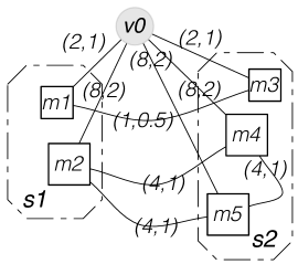
(a) Matrix Storage Graph

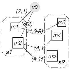
(b) Optimal Plan
without Constraints

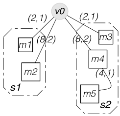
(c) Optimal Plan with
${\mathcal{C}_{r}}^{{\psi_{i}}}(s_{1})\leq 3\wedge{\mathcal{C}_{r}}^{{\psi_{i}}}(s_{2})\leq 6$

Figure 5: Illustrating Matrix Storage Graph & Plan using a Toy Example

IV-C Optimal Parameter Archival Storage

Given the above background, we next address the question of how to best store a collection of model versions, so that the total storage footprint occupied by the large segmented float matrices is minimized while the retrieval performance is not compromised. This recreation/storage tradeoff sits at the core of any version control system. In recent work [11], the authors study six variants of this problem, and show the NP-hardness of most of those variations. However, their techniques cannot be directly applied in PAS, primarily because their approach is not able to handle the group retrieval (co-usage) constraints.

We first introduce the necessary notation, discuss the differences from prior work, and present the new techniques we developed for PAS. In Fig. 4, a model version $v\in V$ consists of time-ordered checkpointed snapshots, $S_{v}={s_{1},...,s_{n}}$. Each snapshot, $s_{i}$ consists of a named list of float matrices $M_{v,i}=\{m_{k}\}$ representing the learned parameters. All matrices in a repository, ${\mathcal{M}}=\bigcup_{v\in V}\bigcup_{s_{i}\in S_{v}}{M_{v,i}}$, are the parameter artifacts to archive. Each matrix $m\in{\mathcal{M}}$ is either stored directly, or is recovered through another matrix $m^{\prime}\in{\mathcal{M}}$ via a delta operator ${\ominus}$, i.e. $m=m^{\prime}\ {\ominus}\ d$, where $d$ is the delta computed using one of the techniques discussed above. In the latter case, the matrix $d$ is stored instead of $m$. To unify the two cases, we introduce a empty matrix ${\nu_{0}}$, and define $\forall{\ominus}\forall m\in{\mathcal{M}},m\ {\ominus}\ {\nu_{0}}=m$.

Definition 1 (Matrix Storage Graph)

Given a repository of model versions $V$, let ${\nu_{0}}$ be an empty matrix, and ${\mathcal{V}}={\mathcal{M}}\cup\{{\nu_{0}}\}$ be the set of all parameter matrices. We denote by ${\mathcal{E}}=\{m_{i}\ {\ominus}\ m_{j}\}\cup\{m_{i}\ {\ominus}\ {\nu_{0}}\}$ the available deltas between all pairs of matrices. Abusing notation somewhat, we also treat ${\mathcal{E}}$ as the set of all edges in a graph where ${\mathcal{V}}$ are the vertices. Finally, let ${\mathcal{G}_{V}({\mathcal{V}},{\mathcal{E}},{c_{s}},{c_{r}})}$ denote the matrix storage graph of $V$, where edge weights ${c_{s}},{c_{r}}:{\mathcal{E}}\mapsto\mathbb{R^{+}}$ are storage cost and recreation cost of an edge respectively.

Definition 2 (Matrix Storage Plan)

Any connected subgraph of ${\mathcal{G}_{V}({\mathcal{V}},{\mathcal{E}})}$ is called a matrix storage plan for $V$, and denoted by ${{\mathcal{P}_{V}}({\mathcal{V}}_{P},{\mathcal{E}}_{P})}$, where ${\mathcal{V}}_{P}={\mathcal{V}}$ and ${\mathcal{E}}_{P}\subseteq{\mathcal{E}}$.

Example 1

In Fig. 5(a), we show a matrix storage graph for a repository with two snapshots, $s_{1}=\{m_{1},m_{2}\}$ and $s_{2}=\{m_{3},m_{4},m_{5}\}$. The weights associated with an edge $e=({\nu_{0}},m_{i})$ reflect the cost of materializing the matrix $m_{i}$ and retrieving it directly. On the other hand, for an edge between two matrices, e.g., $e=(m_{2},m_{5})$, the weights denote the storage cost of the corresponding delta and the recreation cost of applying that delta. In Fig. 5(b) and 5(c), two matrix storage plans are shown.

For a matrix storage plan ${{\mathcal{P}_{V}}({\mathcal{V}}_{P},{\mathcal{E}}_{P})}$, PAS stores all its edges and is able to recreate any matrix $m_{i}$ following a path starting from ${\nu_{0}}$. The total storage cost of ${\mathcal{P}_{V}}$, denoted as ${\mathcal{C}_{s}}({\mathcal{P}_{V}})$, is simply the sum of edge storage costs, i.e. ${\mathcal{C}_{s}}({\mathcal{P}_{V}})=\sum_{e\in{\mathcal{E}}_{P}}{c_{s}}(e)$. Computation of the average snapshot recreation cost is more involved and depends on the retreival scheme used:

• Independent scheme recreates each matrix $m_{i}$ one by one by following the shortest path (${\Upsilon_{{\nu_{0}},m_{i}}}$) to $m_{i}$ from ${\nu_{0}}$. In that case, the recreation cost is simply computed by summing the recreation costs for all the edges along the shortest path.

• Parallel scheme accesses all matrices of a snapshot in parallel (using multiple threads); the longest shortest path from ${\nu_{0}}$ defines the recreation cost for the snapshot.

• Reusable scheme considers caching deltas on the way, i.e., if paths from ${\nu_{0}}$ to two different matrices overlap, then the shared computation is only done once. In that case, we need to construct the lowest-cost Steiner tree ($\mathcal{T}_{{\mathcal{P}_{V}},s_{i}}$) involving ${\nu_{0}}$ and the matrices in the snapshot. However, because multiple large matrices need to be kept in memory simultaneously, the memory consumption of this scheme can be large.

Retrieval Scheme	Recreation ${\mathcal{C}_{r}}^{{\psi}}(\mathcal{P}_{V},s_{i})$	Solution of Prob.1
Independent (${\psi_{i}}$)	$\sum_{m_{j}\in s_{i}}\sum_{e_{k}\in{\Upsilon_{{\nu_{0}},m_{j}}}}{c_{r}}(e_{k})$	Spanning tree
Parallel (${\psi_{p}}$)	$\max_{m_{j}\in s_{i}}\{\sum_{e_{k}\in{\Upsilon_{{\nu_{0}},m_{j}}}}{c_{r}}(e_{k})\}$	Spanning tree
Reusable (${\psi_{r}}$)	$\sum_{e_{k}\in\mathcal{T}_{{\mathcal{P}_{V}},s_{i}}}{c_{r}}(e_{k})$	Subgraph

TABLE III: Recreation Cost of a Snapshot $s_{i}$ ${\mathcal{C}_{r}}({\mathcal{P}_{V}},s_{i})$ in a plan ${\mathcal{P}_{V}}$

PAS can be configured to use any of these options during the actual query execution. However, solving the storage optimization problem with Reusable scheme is nearly impossible; since the Steiner tree problem is NP-Hard, just computing the cost of a solution becomes intractable making it hard to even compare two different storage solutions. Hence, during the storage optimization process, PAS can only support Independent or Parallel schemes.

In the example above, the edges are shown as being undirected indicating that the deltas are symmetric. In general, we allow for directed deltas to handle asymmetric delta functions, and also for multiple directed edges between the same two matrices. The latter can be used to capture different options for storing the delta; e.g., we may have one edge corresponding to a remote storage option, where the storage cost is lower and the recreation cost is higher; whereas another edge (between the same two matrices) may correspond to a local SSD storage option, where the storage cost is the highest and the recreation cost is the lowest. Our algorithms can thus automatically choose the appropriate storage option for different deltas.

Similarly, PAS is able to make decisions at the level of byte segments of float matrices, by treating them as separate matrices that need to be retrieved together in some cases, and not in other cases. This, combined with the ability to incorporate different storage options, is a powerful generalization that allows PAS to make decisions at a very fine granularity.

Given this notation, we can now state the problem formally. Since there are multiple optimization metrics, we assume that constraints on the retrieval costs are provided and ask to minimize the storage.

Problem 1 (Optimal Parameter Archival Storage)

Given a matrix storage graph ${\mathcal{G}_{V}({\mathcal{V}},{\mathcal{E}},{c_{s}},{c_{r}})}$, let $\theta_{i}$ be the snapshot recreation cost budget for each $s_{i}\in S$. Under a retrieval scheme ${\psi}$, find a matrix storage plan ${\mathcal{P}_{V}}^{*}$ that minimizes the total storage cost, while satisfying recreation constraints, i.e.:
   $\operatorname*{minimize}_{{\mathcal{P}_{V}}}{\mathcal{C}_{s}}({\mathcal{P}_{V}});\quad\text{s.t.}\quad\forall s_{i}\in S,{\mathcal{C}_{r}}^{{\psi}}({\mathcal{P}_{V}},s_{i})\leq\theta_{i}$

Example 2

In Fig. 5(b), without any recreation constraints, we show the best storage plan, which is the minimum spanning tree based on ${c_{s}}$ of the matrix storage graph, ${\mathcal{C}_{s}}({\mathcal{P}_{V}})=19$. Under independent scheme ${\psi_{i}}$, ${\mathcal{C}_{r}}^{{\psi_{i}}}({\mathcal{P}_{V}},s_{1})=3$ and ${\mathcal{C}_{r}}^{{\psi_{i}}}({\mathcal{P}_{V}},s_{2})=7.5$. In Fig. 5(c), after adding two constraints $\theta_{1}=3$ and $\theta_{2}=6$, we shows an optimal storage plan ${\mathcal{P}_{V}}^{*}$ satisfying all constraints. The storage cost increases, ${\mathcal{C}_{s}}({\mathcal{P}_{V}}^{*})=24$, while ${\mathcal{C}_{r}}^{{\psi_{i}}}({\mathcal{P}_{V}}^{*},s_{1})=3$ and ${\mathcal{C}_{r}}^{{\psi_{i}}}({\mathcal{P}_{V}}^{*},s_{2})=6$.

Although this problem variation might look similar to the ones considered in recent work [11], none of the variations studied there can handle the co-usage constraints (i.e., the constraints on simultaneously retrieving a group of versioned data artifacts). One way to enforce such constraints is to treat the entire snapshot as a single data artifact that is stored together; however, that may force us to use an overall suboptimal solution because we would not be able to choose the most appropriate delta at the level of individual matrices. Another option would be to sub-divide the retrieval budget for a snapshot into constraints on individual matrices in the snapshot. As our experiments show, that can lead to significantly higher storage utilization. Thus the formulation above is a strict generalization of the formulations considered in that prior work.

Theorem 1

Optimal Parameter Archival Storage Problem is NP-hard for all retrieval schemes in Table III.

Proof:

We reduce Prob.5 in [11] to the independent scheme ${\psi_{i}}$, and Prob.6 in [11] to the parallel scheme ${\psi_{p}}$, by mapping each datasets as vertices in storage graph, and introducing a snapshot holding all matrices with recreation bound $\Theta_{g}$. For reuse scheme ${\psi_{r}}$, it is at least as hard as weighted set cover problem if reducing a set to an edge $e$ with storage cost ${c_{s}}(e)$ as weight, an item to an vertex in ${\mathcal{G}_{V}({\mathcal{V}},{\mathcal{E}})}$, and set recreation budget $\Theta_{g}=\infty$. ∎

Lemma 2

The optimal solution for Problem 1 is a spanning tree when retrieval scheme ${\psi}$ is independent or parallel.

Proof:

Suppose we have a non-tree solution ${\mathcal{P}_{V}}$ satisfying the constraints, and also minimize the objective. Note that parallel and independent schemes are based on shortest path ${\Upsilon_{{\nu_{0}},m}}$ in ${\mathcal{P}_{V}}$ from ${\nu_{0}}$ to each matrix $m$, so the union of each shortest path forms a shortest path tree. If we remove edges which are not in the shortest path tree from the plan to ${\mathcal{P}_{V}}^{\prime}$, it results in a lower objective ${\mathcal{C}_{s}}({\mathcal{P}_{V}}^{\prime})$, but still satisfying all recreation constraints, which leads to a contradiction. ∎

Lemma 2 shows ${\mathcal{P}_{V}}^{*}$ is a spanning tree and connects our problem to a class of constrained minimum spanning tree problems. The above lemma is not true for the reusable scheme (${\psi_{r}})$; snapshot Steiner trees satisfying different recreation constraints may share intermediate nodes resulting in a subgraph solution.

Constrained Spanning Tree Problem: In Problem 1, storage cost minimization while ignoring the recreation constraints leads to a minimum spanning tree (MST) of the storage matrix; whereas the snapshot recreation constraints are best satisfied by using a shortest path tree (SPT). These problems are often referred to as constrained spanning tree problems [17] or shallow-light tree constructions [18], which have been studied in areas other than dataset versioning, such as VLSI designs. Khuller et al. [19] propose an algorithm called LAST to construct such a “balanced” spanning tree in an undirected graph $G$. LAST starts with a minimum spanning tree of the provided graph, traverses it in a DFS manner, and adjusts the tree by changing parents to ensure the path length in constructed solution is within (1+$\epsilon$) times of shortest path in $G$, i.e. ${\mathcal{C}_{r}}(T,v_{i})\leq(1+\epsilon){\mathcal{C}_{r}}({\Upsilon_{{\nu_{0}},v_{i}}},v_{i})$, while total storage cost is within (1+$\frac{2}{\epsilon}$) times of MST. In our problem, the co-usage constraints of matrices in each snapshot form hyperedges over the graph making the problem more difficult.

In the rest of the discussion, we adapt meta-heuristics for constrained MST problems to develop two algorithms: the first one (PAS-MT) is based on an iterative refinement scheme, where we start from an MST and then adjust it to satisfy constraints; the second one is a priority-based tree construction algorithm (PAS-PT), which adds nodes one by one and encodes heuristic in the priority function. Both algorithms aim to solve the parallel and independent recreation schemes, and thus can also find feasible solution for reusable scheme. Due to large memory footprints of intermediate matrices, we leave improving reusable scheme solutions for future work.

Algorithm 1 PAS-MT

0:  ${\mathcal{G}_{V}({\mathcal{V}},{\mathcal{E}},{c_{s}},{c_{r}})}$, snapshots $S$, recreation cost $\{\theta_{i}\geq 0\ |\ s_{i}\in S\}$.

0:  A spanning tree $T$ satisfying constraints $\{{\mathcal{C}_{r}}(T,s_{i})\leq\theta_{i}\}$

1:  let $T=$ MST of ${\mathcal{G}_{V}({\mathcal{V}},{\mathcal{E}})}$;

2:  while unsatisfied constraints $U=\{s_{i}\ |\ {\mathcal{C}_{r}}(T,s_{i})>\theta_{i}\}\neq\emptyset$ do

3:     for each edge $e_{si}=(v_{s},v_{i})\in{\mathcal{E}}-T$ do

4:        calculate $gain(e_{si})$ with Eq. 1 (Eq. 2 for scheme ${\psi_{p}}$)

5:     end for

6:     find $e^{\prime}_{si}=\max\{e_{si}\ |\ gain(e_{si})\}$

7:     break if $gain(e^{\prime}_{si})\leq 0$

8:     swap $(p_{i},v_{i})$ with $e^{\prime}_{si}$: $T=(T-\{(p_{i},v_{i})\})\cup\{e^{\prime}_{si}\}$

9:  end while

10:  return  $T$ unless $U\neq\emptyset$

PAS-MT: The algorithm starts with $T$ as the MST of ${\mathcal{G}_{V}({\mathcal{V}},{\mathcal{E}})}$, and iteratively adjusts $T$ to satisfy the broken snapshot recreation constraints, $U=\{s_{i}|{\mathcal{C}_{r}}(T,s_{i})>\theta_{i}\}$, by swapping one edge at a time. We denote $p_{i}$ as the parent of $v_{i}$, $(p_{i},v_{i})\in T$ and $p_{0}=\phi$, and successors of $v_{i}$ in $T$ as $\mathcal{D}_{i}$. A swap operation on $(p_{i},v_{i})$ to edge $(v_{s},v_{i})\in{\mathcal{E}}-T$ changes parent of $v_{i}$ to $v_{s}$ in $T$.

Lemma 3

A swap operation on $v_{i}$ changes storage cost of ${\mathcal{C}_{s}}(T)$ by ${c_{s}}(p_{i},v_{i})-{c_{s}}(v_{s},v_{i})$, and changes recreation costs of $v_{i}$ and its successors $\mathcal{D}_{i}$ by: ${\mathcal{C}_{r}}(T,v_{i})-{\mathcal{C}_{r}}(T,v_{s})-{c_{r}}(v_{s},v_{i})$.

The proof can be derived from definition of $C_{s}$ and $C_{r}$ by inspection. When selecting edges in ${\mathcal{E}}-T$, we choose the one which has the largest marginal gain for unsatisfied constraints:

$${\psi_{i}}: \max_{(v_{s},v_{i})\in{\mathcal{E}}-T}\{\frac{\sum_{s_{k}\in U}\sum_{v_{j}\in s_{k}\cap\mathcal{D}_{i}}{({\mathcal{C}_{r}}(T,v_{i})-{\mathcal{C}_{r}}(T,v_{s})-{c_{r}}(v_{s},v_{i}))}}{{c_{s}}(v_{s},v_{i})-{c_{s}}(p_{i},v_{i})}\}$$ (1)

$${\psi_{p}}: \max_{(v_{s},v_{i})\in{\mathcal{E}}-T}\{\frac{\sum_{s_{k}\in U}{({\mathcal{C}_{r}}(T,v_{i})-{\mathcal{C}_{r}}(T,v_{s})-{c_{r}}(v_{s},v_{i}))}}{{c_{s}}(v_{s},v_{i})-{c_{s}}(p_{i},v_{i})}\}$$ (2)

The actual formula used is somewhat more complex, and handles negative denominators. Eq. 1 sums the gain of recreation cost changes among all matrices in the same snapshot $s_{i}$ (for the independent scheme), while Eq. 2 uses the max change instead (for the parallel scheme).

The algorithm iteratively swaps edges and stops if all recreation constraints are satisfied or no edge returns a positive gain. A single step examines $|{\mathcal{E}}\ -T|$ edges and $|U|$ unsatisfied constraints, and there are at most $|{\mathcal{E}}|$ steps. Thus the complexity is bounded by $O(|{\mathcal{E}}|^{2}|S|)$.

Algorithm 2 PAS-PT

0:  ${\mathcal{G}_{V}({\mathcal{V}},{\mathcal{E}},{c_{s}},{c_{r}})}$, snapshots $S$, recreation cost $\{\theta_{i}\geq 0\ |\ s_{i}\in S\}$.

0:  A spanning tree $T$ satisfying constraints $\{{\mathcal{C}_{r}}(T,s_{i})\leq\theta_{i}\}$

1:  let $T=\emptyset$ and $Q$ be a priority queue of edges based on ${c_{s}}$

2:  push $\{({\nu_{0}},v_{i})\ |\ v_{i}\in{\mathcal{V}}\}$ in $Q$

3:  while $Q\neq\emptyset$ do

4:     pop $e_{ij}=(v_{i},v_{j})$ from $Q$; let $T=T\cup\{e_{ij}\}$

5:     let constraints satisfaction flag be $\Theta^{e_{ij}}_{satisfy}=true$

6:     for each snapshot constraint $s_{a}\in\{s\ |\ s\in S\wedge v_{j}\in s\}$ do

7:        estimate recreation cost $\hat{\mathcal{C}_{r}}(T,s_{a})$

8:        $\Theta^{e_{ij}}_{satisfy}=false$ and break if $\hat{\mathcal{C}_{r}}(T,s_{a})>\theta_{a}$

9:     end for

10:     if $\Theta^{e_{ij}}_{satisfy}$ is $false$, then $T=T-\{e_{ij}\}$ and goto line 3

11:     pop inner edges of $v_{j}$ $\mathcal{I}^{j}_{T}=\{(v_{k},v_{j})\ |\ v_{k}\in T\}$ from $Q$

12:     push outer edges $\mathcal{O}^{j}_{{\mathcal{E}}-T}=\{(v_{j},v_{k})\ |\ v_{k}\in{\mathcal{E}}-T\}$ to $Q$

13:     for $(v_{k},v_{j})\in T$, change $p_{k}$ improves ${\mathcal{C}_{s}}$, and no worse ${\mathcal{C}_{r}}$ do

14:        swap $(p_{k},v_{k})\in T$ with $(v_{j},v_{k})$

15:     end for

16:  end while

17:  if $T$ is not a spanning tree then

18:     for each $v_{u}\in{\mathcal{V}}-V_{T}$, do $T=T\cup\{e_{0u}=({\nu_{0}},v_{u})\}$

19:     adjust $T$ using PAS-MT heuristic.

20:  end if

21:  return  $T$ if $T$ is a matrix storage plan

PAS-PT: This algorithm constructs a solution by “growing” a tree starting with an empty tree. The algorithm examines the edges in ${\mathcal{G}_{V}({\mathcal{V}},{\mathcal{E}})}$ in the increasing order by the storage cost ${c_{s}}$; a priority queue is used to maintain all the candidate edges and is populated with all the edges from $v_{0}$ in the beginning. At any point, the edges in $Q$ are the ones that connect a vertex $T$, to a vertex outside $T$. Using an edge $e_{ij}=(v_{i},v_{j})$ (s.t., $v_{i}\in V_{T}\wedge v_{j}\in{\mathcal{V}}-V_{T}$) popped from $Q$, the algorithm tries to add $v_{j}$ to $T$ with minimum storage increment ${c_{s}}(e_{ij})$. Before adding $v_{j}$, it examines whether the constraints of affected groups $s_{a}$ (s.t., $v_{j}\in s_{a}$) are satisfied using actual and estimated recreation costs for vertices $\{v_{k}\in s_{a}\}$ in $T$ and ${\mathcal{V}}-T$ respectively; if $v_{k}\in T$, actual recreation cost ${\mathcal{C}_{r}}(T,v_{k})$ is used, otherwise the lower bound of it, i.e. ${c_{r}}({\nu_{0}},v_{k})$ is used as an estimation. We refer the estimation for $s_{a}$ as $\hat{\mathcal{C}_{r}}(T,s_{a})$.

Once an edge $e_{ij}$ is added to $T$, the inner edges $\mathcal{I}^{j}_{T}=\{(v_{k},v_{j})|v_{k}\in T\}$ of newly added $v_{j}$ are dequeued from $Q$, while the outer edges $\mathcal{O}^{j}_{{\mathcal{E}}-T}=\{(v_{j},v_{k})\ |\ v_{k}\in{\mathcal{E}}-T\}$ are enqueued. If the storage cost of existing vertices in $T$ can be improved (i.e., ${\mathcal{C}_{s}}(T,v_{k})>{c_{s}}(v_{k},v_{j})$), and recreation cost is not more (i.e. ${\mathcal{C}_{r}}(T,v_{k})\geq{\mathcal{C}_{r}}(T,v_{j})+{c_{r}}(v_{k},v_{j})$), then the parent $p_{k}$ of $v_{k}$ in T is replaced to $v_{j}$ via the swap operation, which obviously decreases the storage cost and affected group recreation cost.

The algorithm stops if $Q$ is empty and $T$ is a spanning tree. In the case when $Q$ is empty but $V_{T}\subset{\mathcal{V}}$, an adjustment operation on $T$ to increase storage cost and satisfy the group recreation constraints is performed. For each $v_{u}\in{\mathcal{V}}-V_{T}$, we append it to ${\nu_{0}}$, then in each unsatisfied group $s_{i}$ that $v_{u}$ belongs to, optimally, we want to choose a set of $\{v_{g}\}\subseteq s_{i}\cap T$ to change their parents in $T$, such that the decrement of storage cost is minimized while recreation cost is satisfied. The optimal adjustment itself can be viewed as a knapsack problem with extra non-cyclic constraint of $T$, which is NP-hard. Instead, we use the same heuristic in Eq. 1 to adjust $v_{g}\in s_{i}\cap T$ one by one by replacing its parent $p_{g}$ to $v_{s}$ until the group constraint in $s_{i}$ is satisfied. As before, the parallel scheme ${\psi_{p}}$ differs from independent case ${\psi_{i}}$ in the adjustment operator using Eq. 2. The complexity of this algorithm is $O(|{\mathcal{E}}|^{2}|S|)$.

IV-D Model Evaluation Scheme in PAS

Model evaluation, i.e., applying a DNN forward on a data point to get the prediction result, is a common task to explore, debug and understand models. Given a PAS storage plan, an dlv eval query requires uncompressing and applying deltas along the path to the model. We develop a novel model evaluation scheme utilizing the segmented design, that progressively accesses the low-order segments only when necessary, and guarantees no errors for arbitrary data points.

The basic intuition is that: when retrieving segmented parameters, we know the minimum and maximum values of the parameters (since higher order bytes are retrieved first). If the prediction result is the same for the entire range of those values, then we do not need to access the lower order bytes. However, considering the high dimensions of parameters, non-linearity of the DNN model, unknown full precision value when issuing the query, it is not clear if this is feasible.

We define the problem formally, and illustrate the determinism condition that we use to develop our algorithm. Our technique is inspired from theoretical stability analysis in numerical analysis. We make the formulation general to be applicable to other prediction functions. The basic assumption is that the prediction function returns a vector showing relative strengths of the classification labels, then the dimension index with the maximum value is used as the predicted label.

Problem 2 (Parameter Perturbation Error Determination)

Given a prediction function $\mathcal{F}(d,W):\mathbb{R}^{m}\times\mathbb{R}^{n}\mapsto\mathbb{R}^{c}$, where $d$ is the data and $W$ are the learned weights, the prediction result $c_{d}$ is the dimension index with the highest value in the output $o\in\mathbb{R}^{c}$. When $W$ value is uncertain, i.e., each $w_{i}\in W$ in known to be in the range $[w_{i,\min},w_{i,\max}]$, determine whether $c_{d}$ can be ascertained without error.

When $W$ is uncertain, the output $o$ is uncertain as well. However, if we can bound the individual entries in $o$, then the following condition is an applicable necessary condition for determining error:

Lemma 4

Let $o_{i}\in o$ vary in range $[o_{i,\min},o_{i,\max}]$. If $\exists k$ such that $\forall i,\ o_{k,\min}>o_{i,\max}$, then prediction result $c_{d}$ is $k$.

Next we illustrate a query procedure, that given data $d$, evaluates a DNN with weight perturbations and determines the output perturbation on the fly. Recall that DNN is a nested function (Sec. II), we derive the output perturbations when evaluating a model while preserving perturbations step by step:

$$x_{0,k} =\sum_{j}W_{0,k,j}d_{j}+b_{0,k} x_{0,k,\min} =\sum_{j}\min\{W_{0,k,j}d_{j}\}+\min\{b_{0,k}\}$$

$$x_{0,k,\max} =\sum_{j}\max\{W_{0,k,j}d_{j}\}+\max\{b_{0,k}\}$$

Next, activation function $\sigma_{0}$ is applied. Most of the common activation functions are monotonic function $\mathbb{R}\mapsto\mathbb{R}$, (e.g. sigmoid, ReLu), while pool layer functions are $\min$, $\max$, avg functions over several dimensions. It is easy to derive the perturbation of output of the activation function, $[f_{0,k,\min},f_{0,k,\max}]$. During the evaluation query, instead of 1-D actual output, we carry 2-D perturbations, as the actual parameter value is not available. Nonlinearity decreases or increases the perturbation range. Now the output perturbation at $f_{i}$ can be calculated similarly, except now both $W$ and $f_{i-1}$ are uncertain:

$$x_{i,k} =\sum_{j}W_{i,k,j}f_{i-1,j}+b_{i,k} x_{i,k,\min} =\sum_{j}\min\{W_{i,k,j}f_{i-1,j}\}+\min\{b_{i,k}\}$$

$$x_{i,k,\max} =\sum_{j}\max\{W_{i,k,j}f_{i-1,j}\}+\max\{b_{i,k}\}$$

Applying these steps iteratively until last layer, we can then apply Lemma 4, the condition of error determinism, to check if the result is correct. If not, then lower order segments of the float matrices are retrieved, and the evaluation is re-performed.

This progressive evaluation query techniques dramatically improve the utility of PAS, as we further illustrate in our experimental evaluation. Note that, other types of queries, e.g., matrix plots, activation plots, visualizations, etc., can often be executed without retrieving the lower-order bytes either.

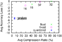
(a) Compression-Accuracy Tradeoff
for Float Representation Schemes

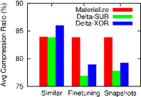
(b) Compression Performance for
Different Delta Schemes & Models

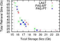
(c) PAS Optimal Archival Storage
Algorithms Results for SD

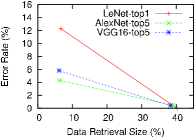
(d) Progressive Evaluation Query
Processing Using High-Order Bytes

Figure 6: Evaluation Results for PAS

V Evaluation Study

ModelHub is designed to work with a variety of deep learning backends; our current prototype interfaces with caffe [3] through a wrapper that can extract caffe training logs, and read and write parameters for training. We have also built a custom layer in caffe to support progressive queries. The dlv command-line suite is implemented as a Ruby gem, utilizing git as internal VCS and sqlite3 and PAS as backends to manage the set of heterogeneous artifacts in the local client. PAS is built in C++ with gcc 5.4.0. All experiments are conducted on a Ubuntu Linux 16.04 machine with an 8-core 3.0GHz AMD FX-380 processor, 16GB memory, and NVIDIA GTX 370 GPU. We use zlib for compression; unless specifically mentioned, the compression level is set to 6. When wrapping and modifying caffe, the code base version is rc3.

In this section, we present a comprehensive evaluation with real-world and synthetic datasets aimed at examining our design decisions, differences of configurations in PAS, and performance of archiving and progressive query evaluation techniques proposed in earlier sections.

V-A Dataset Description

Real World Dataset: To study the performance of PAS design decisions, float representations, segmented float storage, delta encoding and overall compression performance, we use a collection of shared caffe models published in caffe repository or Model Zoo. In brief, LeNet-5 [6] is a convolutional DNN with 431k parameters. The reference model has 0.88% error rate on MNIST. AlexNet [7] is a medium-sized model with 61 million parameters, while VGG-16 [8] has 1.9 billion parameters. Both AlexNet and VGG-16 are tested on ILSVRC-2012 dataset. The downloaded models have 43.1%, and 31.6% top-1 error rate respectively. Besides, to study the delta performance on model repositories under different workloads (i.e., retraining, fine-tuning): we use CNN-S/M/F [20], a set of similar models developed by VGG authors to study model variations. These models are similar to VGG in architecture, and retrained from scratch; for fine-tuning, we use VGG-Salient [21] a fine-tuning VGG model which only changes last full layer.

Synthetic Datasets: Lacking sufficiently fine-grained real-world repositories of models, to evaluate performance of parameter archiving algorithms, we developed an automatic modeler to enumerate models and hyperparameters to produce a dlv repository. We generated a synthetic dataset (SD): simulating a modeler who is enumerating models to solve a face recognition task, and fine-tuning a trained VGG. SD results in similar DNNs and relatively similar parameters across the models. The datasets are shared online.

To elaborate, the automation is driven by a state machine that applies modeling practices from the real world. The modeler updates the VGG network architecture slightly and changes VGG object recognition goal to a face prediction task (prediction labels changed from 1000 to 100, so the last layer is changed); various fine-tuning hyperparameter alternations are applied by mimicking practice [22]. SD in total has 54 model versions, each of which have 10 snapshots. A snapshot has 16 parametric layers and a total of $1.96\times 10^{10}$ floats.

V-B Evaluation Results

Float Representation & Accuracy: We show the effect of different float encoding schemes on the compression and accuracy in Fig. 6(a); this is a tradeoff that the user often needs to consider when configuring ModelHub to save a model. In Fig. 6(a), for each scheme, we plot the average compression ratio versus the average accuracy drop when applying PAS float schemes on the three real world models. Here, random and uniform denote two standard quantization schemes. As we can see, we can get very high compression ratios (a factor of 20 or so) without a significant loss in accuracy, which may be acceptable in many scenarios.

Delta Encoding & Compression Ratio Gain: Next we study the usefulness of delta encoding in real world models in the following scenarios: a) Similar: latest snapshots across similar models (CNN-S/M/F, VGG-16); b) Fine-tuning: fine-tuning models (VGG-16, VGG-Salient); and c) Snapshots: snapshots for the same VGG models in SD between iterations. In Fig. 6(b), for different delta schemes, namely, storing original matrices (Materialize), arithmetic subtraction (Delta-SUB), and bitwise XOR diff (Delta-XOR), the comparison is shown (i.e., we show the results of compressing the resulting matrices using zlib). The figure shows the numbers under lossless compression scheme (float 32), which has the largest storage footprint.

As we can see, delta scheme is not always good, due to the non-convexity and high entropy of parameters. For models under similar architectures, storing materialized original parameters is often better than applying delta encoding. With fine-tuning and nearby snapshots, the delta is always better, and arithmetic subtraction is consistently better than bitwise XOR. We saw similar results for many other models. These findings are useful for PAS implementation decisions, where we only perform delta between nearby snapshots in a single model, or for the fine-tuning setting among different models.

Optimal Parameter Archival Storage: We study the optimality and scalability of PAS-PT and PAS-MT with the baseline LAST [19] on the optimal parameter archival problem. We use SD here, from which we derive nearby snapshot deltas as well as model-wise deltas among the latest snapshots. For the access frequencies, in practice, the modeler tends to access better models more frequently than bad ones. We use multinomial distributions based on model accuracies to mimic the behavior. As LAST cannot handle the co-usage constraints, to have a reasonable baseline, we decompose the co-usage constraint to be proportional to each layer matrix size. The performance of the algorithms is shown in Fig. 6(c). Two dotted lines are the minimum possible storage cost (MST) and the recreation cost (SPT) for the independent scheme in version graph. Each data point is a storage plan found by the algorithms given a recreation cost constraint. As we can see, PAS algorithms (PT and MT) consistently perform better than LAST. The reason is both of them consider the constraints as a group and thus choose better storage plans.

Progressive Query Evaluation: We study the efficiency of the progressive evaluation technique using perturbation error determination scheme on real world models (LeNet, AlexNet, VGG16) and their corresponding datasets. The original parameters are 4-byte floats, which are archived in segments in PAS. We modify caffe implementation of involved layers and pass two additional blobs (min/max errors) between layers. The perturbation error determination algorithm uses high order segments, and answers eval query on the whole test dataset. The algorithm determines whether top-k (1 or 5) result needs lower order bytes (i.e., matched index value range overlaps with $k+1$ index value range).

The result is summarized in Fig. 6(d). The y-axis shows the error rate, i.e., the percentage of test dataset that may have perturbation errors due to low precision. The x-axis shows the percentage of data that needs to be retrieved (i.e., 2 bytes or 1 byte per float). As one can see, the prediction errors requiring full precision lower-order bytes are very small. The less high-order bytes used, higher the chance of potential errors. The consistent result of progressive query evaluation on real models supports our design decision of segmented float storage.

VI Related Work

Machine Learning Systems: There have been several high-profile deep learning systems in recent years, but those typically focus on the training aspects (e.g., on distributed training, how to utilize GPUs or allow symbolic formulas, etc.) [3, 4, 23, 24, 25]. The data and lifecycle management challenges discussed above have been largely ignored so far, but are becoming critical as the use of deep learning permeates through a variety of application domains, since those pose a high barrier to entry for many potential users. In the database community, there has been increasing work on developing general-purpose systems for supporting machine learning, including pushing predictive models into databases [26, 27], accelerating tasks using database optimizing methods [2, 28], and managing modeling lifecycles and serving predictive models in advanced ways [29, 30]. ModelHub is motivated by similar principles; aside from a focus on DNNs, it also supports versioning as a first-class construct [10] which differentiates it from that work.

DNN Compression: There has been increasing interest on compressing DNN models, motivated in part by the need to deploy them on devices with simple instruction sets, low memory, and/or energy constraints [13, 31, 32]. However, the goal of those works is simplify the model in a lossy manner with as little loss of accuracy as possible, which makes this work orthogonal to the archival approach we take in ModelHub; in fact, simplified models are likely to compress much better, magnifying the gains of our approach as our experimental results show. Further, these methods often require heavy retraining or expensive computations (k-means, SVD, etc.) to derive simpler models, which makes them too heavyweight in an interactive setting for which DLV is designed.

DNNs with Low Precision Floats: Low precision floats are exploited in accelerating training and testing systems [12, 32, 33], showing techniques and empirical results when training, testing DNN with limited precisions. ModelHub differs from their work by exploiting parameters archiving, and use segmented floats to answer lifecycle modeling queries.

Stability Analysis Results Stability analysis of DNN is studied in the literature [34, 35, 36], where the problem setting is perturbation analysis regardless specific data, rather focus on statistical measures of stability. ModelHub uses basic perturbation analysis techniques and focus on novel progressive query answering in a segmented float storage.

VII Conclusion and Future Work

In this paper, we described some of the key data management challenges in learning, managing, and adjusting deep learning models, and presented our ModelHub system that attempts to address those challenges in a systematic fashion. The goals of ModelHub are multi-fold: (a) to make it easy for a user to explore the space of potential models by tweaking the network architecture and/or the hyperparameter values, (b) to minimize the burden in keeping track of the metadata including the accuracy scores and the fine-grained results, and (c) to compactly store a large number of models and constituent snapshots without compromising on query or retrieval performance. We presented several high-level abstractions, including a command-line version management tool and a domain-specific language, for addressing the first two goals. Anecdotal experience with our early users suggests that both of those are effective at simplifying the model exploration tasks. We also developed a read-optimized parameter archival storage for storing the learned weight parameters, and designed novel algorithms for storage optimization and for progressive query evaluation. Extensive experiments on real world and synthetic models verify the design decisions we made and demonstrate the advantages of proposed techniques.

References

- [1] Y. LeCun, Y. Bengio, and G. Hinton, “Deep learning,” Nature, 2015.
- [2] C. Zhang, A. Kumar, and C. Ré, “Materialization optimizations for feature selection workloads,” in SIGMOD, 2014.
- [3] Y. Jia et al., “Caffe: Convolutional architecture for fast feature embedding,” in ACM MM, 2014.
- [4] M. Abadi et al., “TensorFlow: A system for large-scale machine learning,” in OSDI, 2016.
- [5] L. Bottou, “Stochastic gradient descent tricks,” in Neural Networks: Tricks of the Trade. Springer, 2012, pp. 421–436.
- [6] Y. LeCun et al., “Handwritten digit recognition with a back-propagation network,” in NIPS, 1990.
- [7] A. Krizhevsky, I. Sutskever, and G. E. Hinton, “Imagenet classification with deep convolutional neural networks,” in NIPS, 2012.
- [8] K. Simonyan and A. Zisserman, “Very deep convolutional networks for large-scale image recognition,” CoRR, vol. abs/1409.1556, 2014.
- [9] K. He, X. Zhang, S. Ren, and J. Sun, “Deep residual learning for image recognition,” in CVPR, 2016.
- [10] A. Bhardwaj et al., “DataHub: Collaborative data science and dataset version management at scale,” in CIDR, 2015.
- [11] S. Bhattacherjee, A. Chavan, S. Huang, A. Deshpande, and A. Parameswaran, “Principles of dataset versioning: Exploring the recreation/storage tradeoff,” PVLDB, 2015.
- [12] V. Vanhoucke, A. Senior, and M. Z. Mao, “Improving the speed of neural networks on CPUs,” in Proc. Deep Learning and Unsupervised Feature Learning NIPS Workshop, 2011.
- [13] S. Han et al., “Deep compression: Compressing deep neural networks with pruning, trained quantization and huffman coding,” in ICLR, 2016.
- [14] M. Courbariaux et al., “Training deep neural networks with low precision multiplications,” arXiv preprint arXiv:1412.7024, 2014.
- [15] E. R. Schendel et al., “Isobar preconditioner for effective and high-throughput lossless data compression,” in ICDE, 2012.
- [16] S. Bhattacherjee, A. Deshpande, and A. Sussman, “Pstore: an efficient storage framework for managing scientific data,” in SSDBM, 2014.
- [17] N. Deo and N. Kumar, “Computation of constrained spanning trees: A unified approach,” in Network Optimization, 1997.
- [18] A. B. Kahng and G. Robins, On optimal interconnections for VLSI. Springer Science & Business Media, 1994, vol. 301.
- [19] S. Khuller, B. Raghavachari, and N. Young, “Balancing minimum spanning trees and shortest-path trees,” Algorithmica, 1995.
- [20] K. Chatfield et al., “Return of the devil in the details: Delving deep into convolutional nets,” in BMVC, 2014.
- [21] J. Zhang, S. Ma, M. Sameki, S. Sclaroff, M. Betke, Z. Lin, X. Shen, B. Price, and R. Mech, “Salient object subitizing,” in CVPR, 2015.
- [22] R. Girshick, “Fast R-CNN,” in ICCV, 2015.
- [23] J. Dean et al., “Large scale distributed deep networks,” in NIPS, 2012.
- [24] T. Chilimbi et al., “Project ADAM: Building an efficient and scalable deep learning training system,” in OSDI, 2014.
- [25] W. Wang et al., “Singa: Putting deep learning in the hands of multimedia users,” in ACM MM, 2015.
- [26] M. Akdere, Cetintemel et al., “The case for predictive database systems: Opportunities and challenges.” in CIDR, 2011.
- [27] X. Feng, A. Kumar, B. Recht, and C. Ré, “Towards a unified architecture for in-rdbms analytics,” in SIGMOD, 2012.
- [28] A. Kumar, J. Naughton, and J. M. Patel, “Learning generalized linear models over normalized data,” in SIGMOD, 2015.
- [29] M. Vartak et al., “Supporting fast iteration in model building,” in LearningSys, 2015.
- [30] D. Crankshaw, X. Wang, J. E. Gonzalez, and M. J. Franklin, “Scalable training and serving of personalized models,” in LearningSys, 2015.
- [31] E. L. Denton et al., “Exploiting linear structure within convolutional networks for efficient evaluation,” in NIPS, 2014.
- [32] W. Sung, S. Shin, and K. Hwang, “Resiliency of deep neural networks under quantization,” arXiv preprint arXiv:1511.06488, 2015.
- [33] S. Gupta, A. Agrawal, K. Gopalakrishnan, and P. Narayanan, “Deep learning with limited numerical precision,” in ICML, 2015.
- [34] M. Stevenson et al., “Sensitivity of feedforward neural networks to weight errors,” IEEE Trans. Neural Networks, vol. 1, 1990.
- [35] X. Zeng et al., “Sensitivity analysis of multilayer perceptron to input and weight perturbations,” IEEE Trans. Neural Networks, vol. 12, 2001.
- [36] J. Yang, X. Zeng, and S. Zhong, “Computation of multilayer perceptron sensitivity to input perturbation,” Neurocomputing, 2013.