Optical Spectra of Ultracool Dwarfs
with the Southern African Large Telescope.

C. Koen¹, B. Miszalski^2,3, P. Väisänen^2,3 and T. Koen³
1 Department of Statistics, University of the Western Cape, Private Bag X17, Bellville, 7535 Cape, South Africa
ckoen@uwc.ac.za

2 South African Astronomical Observatory, PO Box 9, Observatory, 7935 Cape, South Africa
3 Southern African Large Telescope, PO Box 9, Observatory, 7935 Cape, South Africa

ABSTRACT. New spectra of 81 ultracool dwarfs (spectral types M7 and later) are discussed. Spectral classifications of 49 objects are available in the literature, while 32 objects are newly classified. The known spectral types were used to test an automated classification scheme, which relies primarily on template fitting, supplemented by matching of spectral indices calibrated against the template spectra. An attempt was made to quantify the uncertainty in the spectral types, which is generally better than two subclasses. Objects for which spectral types differ by more than one subclass from the literature classifications are discussed individually. Discrepancies between automated classifications based on respectively template fitting and spectral index matching, may be useful for flagging objects with unusual spectra. Aside from the 32 first-time classifications, alternative classifications are presented for 32 previously classified dwarfs. Very large (equivalent width greater than 130 Å) H$\alpha$ flares are reported for the known ultracool dwarf binary 2MASS J15200224-4422419; curiously, the object does not appear to have quiescent emission lines. Non-zero equivalent width measurements are listed for a further 29 objects.

Key words: stars: low-mass - stars: flare - stars: brown dwarfs

1 INTRODUCTION

This paper presents far red (6300-8800 Å ) spectroscopic observations of 81 ultracool dwarfs (UCDs), i.e. objects (stars and brown dwarfs) with spectral types of M7 or later. The aims of this ongoing project are to (i) obtain classification spectra of photometrically selected candidate UCDs; (ii) obtain optical spectra of UCDs for which only NIR spectral classifications have been published; (iii) to revisit confirmed UCDs in order to investigate the prevalence of spectral variability; and (iv) to obtain H$\alpha$ equivalent widths of a large sample of UCDs.

A consequence of the low temperatures of UCDs is that objects with these spectral types are much brighter at infrared wavelengths, which has no doubt contributed to the large number of near infrared (NIR) spectra which have been published – the comprehensive websites http://spider.ipac.caltech.edu/staff/davy/ARCHIVE/index.shtml and https://jgagneastro.wordpress.com/list-of-ultracool-dwarfs/ contain references to hundreds of examples. However, spectral classification for all stars and brown dwarfs that could be reasonably detected optically (which includes late M and L type UCDs), was historically developed for spectra taken in the optical (e.g. Kirkpatrick et al. 1999). Added to this are the facts that the spectral sequence is not as obvious in the NIR, and that NIR colours at a given spectral type show considerable scatter – see Allers & Liu (2013) for a discussion. As a result, classification based on NIR spectra is less certain (e.g. Luhman et al. 2003, Lodieu et al. 2005). [Note though that although definitive classifications may not always be obtainable from NIR spectra, these do contain further information about conditions in UCD atmospheres, since different physical environments are sampled than by optical spectroscopy (Kirkpatrick 2009)].

Modest spectral resolution is sufficient to obtain H$\alpha$ equivalent widths, and this is exploited in the study reported below. A recent discussion of magnetic activity in UCDs can be found in Metodieva et al. (2015), which is also a source of references to earlier work (see also section 5 of this paper). The authors provide a plot of the activity indicator log $L_{{\rm H}\alpha}/L_{\rm bol}$ against spectral type, based on their own observations and values taken from the literature. There is a clear decrease in mean activity, the later the spectral type. Since relatively strong magnetic fields have been observed in some late M/early L UCDs (e.g. Williams, Cook & Berger 2014, and references therein), the activity decrease may be due to the inability of largely neutral atmospheres to manipulate the magnetic fields. An exception to this general trend is discussed in section 5, in the form of an enormous flare associated with a binary UCD consisting of two early L dwarfs. It is particularly noteworthy that other visits to this object did not reveal any signs of quiescent H$\alpha$ emission.

The paper presents spectra of 81 objects, with 32 new classifications of photometric UCD candidates taken from Folkes et al. (2012). Spectral types for the remaining 49 UCDs were available in the literature, and were used to thoroughly test our classification software. Spectral typing is performed by comparison of SALT spectra to sets of template spectra, and rely on matching either continuum shapes (template fitting) or sets of spectral indices.

2 OBSERVATIONS

We obtained spectroscopic observations of many candidates with the Robert Stobie Spectrograph (RSS; Burgh et al. 2003; Kobulnicky et al. 2003) on the queue-scheduled Southern African Large Telescope (SALT; Buckley, Swart & Meiring 2006; O’Donoghue et al. 2006) under programmes 2014-1-RSA-003, 2014-2-MLT-003 and 2015-1-MLT-003. The observing strategy involved providing a large surplus of targets with relatively short exposure times of 2$\times$600 s across large parts of the sky such that observations could readily be taken during any gaps in the SALT queue. This filler program approach had relatively loose constraints on the seeing and sky conditions to further maximise the chance that observations would be taken. A red RSS configuration was adopted with the PG900 grating covering the wavelength range of $\sim$6320–9268 Å. The slit widths varied between 1.00, 1.25 and 1.50 arcsec, depending on the target brightness, yielding resolving powers of 2128, 1703 and 1419, respectively, at the central wavelength of 7828 Å. The reciprocal dispersion was 0.94 Å pixel^-1.

Table 1 gives the Two Micron All Sky Survey (2MASS) point source catalogue designation (Skrutskie et al. 2006), date and exposure time of the observations used in this paper. A neon-argon or xenon arc lamp reference spectrum was taken after each sequence of science exposures, as well as five internal flat-field lamps exposures. Data reduction was performed using iraf on the SALT pipeline data products processed by pysalt (Crawford et al. 2010). The data were trimmed, leaving only the central region of each frame, and then cleaned of cosmic ray events using lacosmic (van Dokkum 2001). The CCD chips were interpolated over before flat-fielding the data by a normalised average flat-field that had first been divided by a smoothed median of itself. Wavelength calibration was performed using the standard iraf tasks identify, reidentify, fitcoords and transform. Before extracting one-dimensional spectra with apall, all acquisition images from SALT were carefully inspected, along with images from the SuperCOSMOS Sky Survey (Hambly et al. 2001) and 2MASS (Skrutskie et al. 2006), to ensure the correct target was on the slit and to identify its spatial position on the CCD. This step was necessary given the challenging acquisition task of acquiring very red targets with high proper motions in sometimes very crowded fields. A relative flux calibration was applied to all spectra using spectrophotometric standards taken during each semester of observations in the standard fashion. The wavelength range was then trimmed to $\sim$6320–8800 Å to remove the reddest wavelengths affected by second-order contamination introduced by the grating. Where possible a combined spectrum for each object was created from a simple average of the two or three spectra taken during each individual observation.

H$\alpha$ equivalent widths (EWs) were measured by fitting a Gaussian profile to the emission line using the IRAF task SPLOT.

3 SPECTRAL CLASSIFICATION: PROCEDURES

Before analysis, the spectral regions 6860-6940, 7590-7680, 7300-7365 and 8310-8365 Å were removed; the first two are affected by the telluric Fraunhofer A and B features, the latter two include the gaps between CCD detectors.

3.1 Template fitting (TF)

The primary classification tool was the fitting of template spectra: the overall shapes of the spectra are more resistant to the effects of noise, and less affected by secondary effects such as gravity variations. Templates were obtained from Bochanski et al. (2007) (M dwarfs) and Schmidt et al. (2014) (L dwarfs). The wavelength spacing of the L dwarf templates varies from 0.36 Å for early L, to 1.1 Å for late L. This is similar to the 0.94 Å spacing of our spectra, so that template spectra were simply interpolated. M dwarf template spectra are given at a finer wavelength resolution of 0.1 Å  and these were binned to 0.9 Å for comparison with the SALT spectra.

Assuming that flux calibrations have been made, matching SALT and template spectra consisted solely of determining a scale factor $\beta$. This is determined by least squares as

$$\beta=\sum_{\lambda}F_{S}(\lambda)F_{t}(\lambda)/\sum_{\lambda}F^{2}_{t}(\lambda)$$

where the subscripts $S$ and $t$ respectively denote the SALT and template spectra. The “figure of merit” is the sum of squares

$$SS_{1}=\sum_{\lambda}[F_{S}(\lambda)-\beta F_{t}(\lambda)]^{2}\;.$$ (1)

3.2 Spectral indices matching

Secondary classification tools are based on spectral indices. Twenty two indices were taken from Reid, Hawley & Gizis (1995), Kirkpatrick et al. (1999), Hawley et al. (2002) and Cruz et al. (2009) – see Table 2. For the first 17 indices, the ratios of the fluxes in the two wavelength intervals were calculated. The last four indices are defined as the mean flux over the first interval, divided by the mean of the fluxes over the two denominator intervals. The CaH1 index was calculates as described in Reid et al. (1995), by interpolating the mean flux between the two denominator intervals.

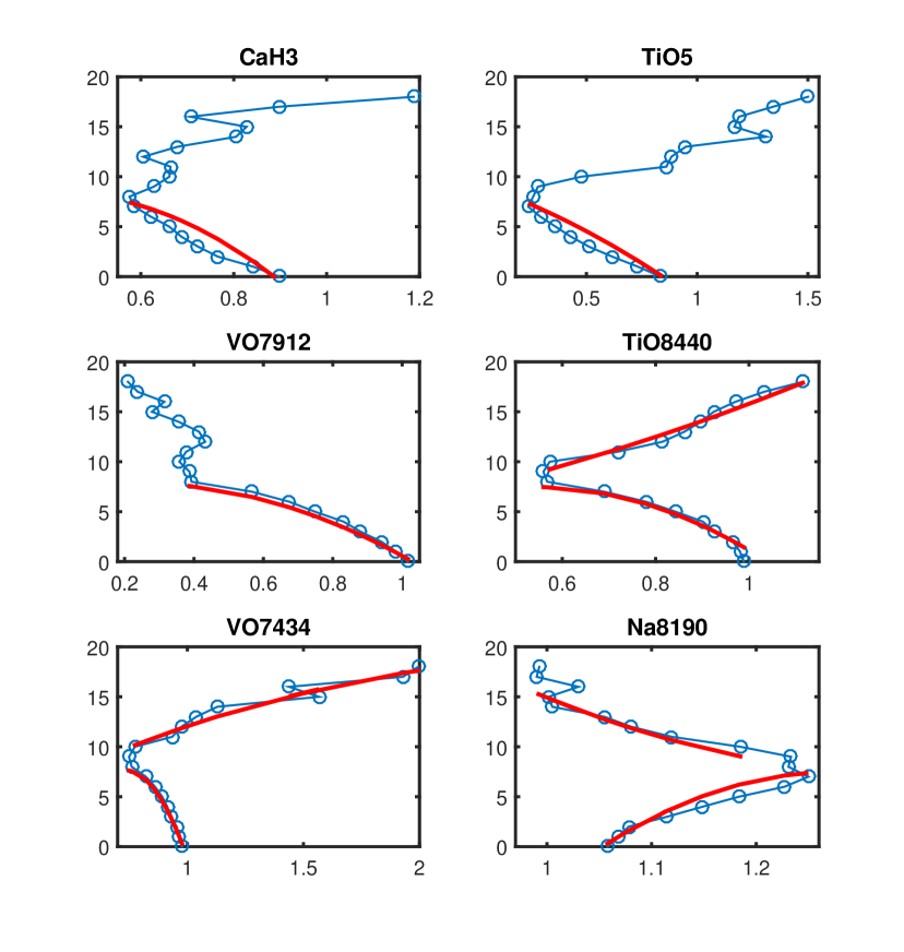
Figure 1: The six spectral indices calibrated by Hawley et al. (2002) (smooth solid lines) and the values obtained from the spectral templates (open circles). Spectral class is plotted on the vertical axes, running from 0 (M0) to 18 (L8).

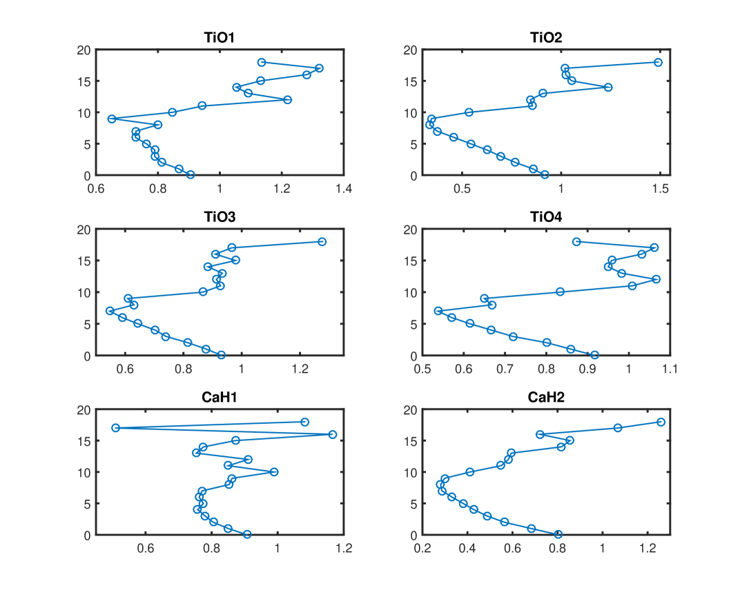
Figure 2: Numerical values of six of the spectral indices defined in Table 2, calculated from the spectral templates.

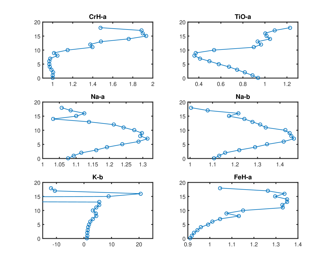
Figure 3: Numerical values of six of the spectral indices defined in Table 2, calculated from the spectral templates.

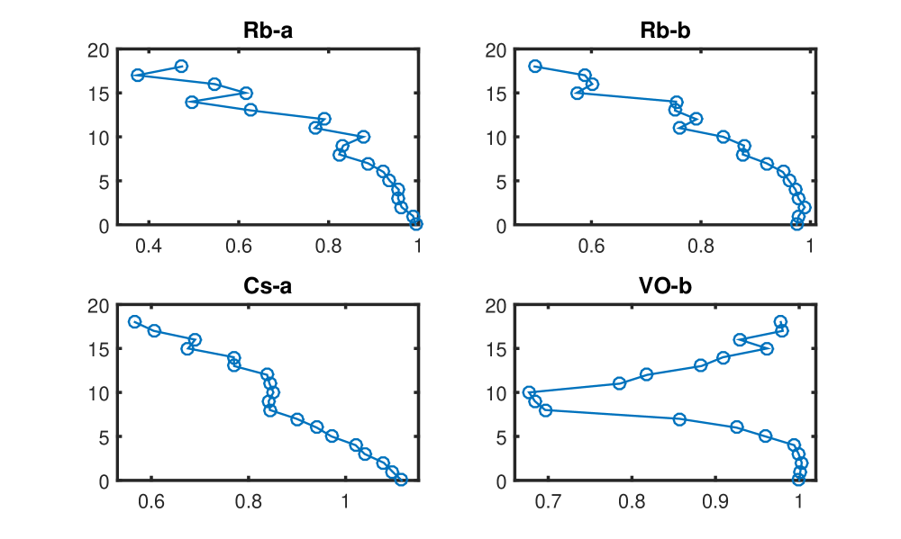
Figure 4: Numerical values of four of the spectral indices defined in Table 2, calculated from the spectral templates.

The indices were calibrated by calculating each of them for all of the 19 template spectra. The results are in Figs. 1-4, the first of which also shows (as red lines) digitisations of the fits plotted in fig. 3 of Hawley et al. (2002). Inspection of the diagrams shows that the late L template spectra are not of sufficient quality to calibrate the K-b index. Furthermore, it is not clear whether the calculated CaH1 index is accurate enough to be usable – if it is, it may be of limited utility anyway, since the plot suggests that its discriminatory power may be limited. The K-b and CaH1 indices were therefore not used for classification.

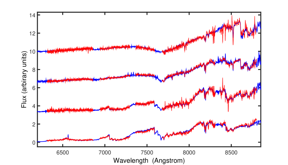
Figure 6: Representative examples of the fits of SALT spectra (red) to templates (blue). From top to bottom, 2M 2252-1730 (L5); 2M 0128-5545 (L3); 2M 1523-2347 (L0); and 2M 1308-4925 (M7).

To elaborate: the CaH1 index involves fluxes in the wavelength interval 6345-6420 Å, some 250 Å blueward of the wavelength ranges of all other indices in Table 2. Given the extreme dearth of blue flux emitted by UCDs with mid and late L spectral types (see e.g. Fig. 6), it is no surprise that it is difficult to accurately calibrate the CaH1 over the entire spectral range considered in this paper. At first sight the K-b index may be expected to be reliable at later spectral types. However, the broad K I absorption trough due to the doublet at 7665 and 7699 Å deepens with deceasing temperature and by mid L the flux level in this part of the spectrum is comparable to that on which the CaH1 index is based. In some of the later type template spectra fluxes in the wavelength ranges of these two indices are close to zero, or even negative.

Noise sometimes leads to calculated indices being outside the ranges covered by the calibrations. If the discrepancy is a few percent, then it seems plausible to associate the index with the closest spectral class. (For example, if TiO4=0.5, the estimated spectral class is M7). Otherwise, if the margin is too large, the index is rejected.

The most straightforward classification based on indices is to search for the spectral type with the best overall agreement between observed and calibrated indices:

$$\min_{t}[SS_{2}(t)]=\min_{t}\sum_{j}[I_{j}({\rm observed})-I_{j}({\rm template}\;t)]^{2}$$ (2)

where $I_{j}$ denotes spectral index $j$, and $t$ again indexes the template spectra. An alternative which is more resistant to outlying index values is

$$\min_{t}\sum_{j}|I_{j}({\rm observed})-I_{j}({\rm template}\;t)|\;.$$ (3)

In order to place all indices on equal footing the $I_{j}$ are standardised such $0\leq I_{j}({\rm template})\leq 1$ (i.e. the minimum value for the particular template index is subtracted, and the result is divided by the range spanned by the index).

Approximate standard errors of the spectral indices follow from the delta method as

$${\rm S.E.}(I_{j}) = \left[\frac{{\rm var}(F_{n})}{\ell_{n}\overline{F}_{d}^{2}}+\frac{\overline{F}_{n}^{2}{\rm var}(F_{d})}{\ell_{d}\overline{F}_{d}^{4}}\right]^{1/2}\;\;\;\;\;j=1-17$$ (4)

$$= 13\left\{\frac{{\rm var}(F_{n})}{\ell_{n}(7\overline{F}_{d1}+6\overline{F}_{d2})^{2}}+\frac{\overline{F}_{n}^{2}}{(7\overline{F}_{d1}+6\overline{F}_{d2})^{4}}\left[\frac{{7^{2}\rm var}(F_{d1})}{\ell_{d1}}+\frac{6^{2}{\rm var}(F_{d2})}{\ell_{d2}}\right]\right\}^{1/2}\;\;\;\;\;j=18$$

$$= 2\left\{\frac{{\rm var}(F_{n})}{\ell_{n}(\overline{F}_{d1}+\overline{F}_{d2})^{2}}+\frac{\overline{F}_{n}^{2}}{(\overline{F}_{d1}+\overline{F}_{d2})^{4}}\left[\frac{{\rm var}(F_{d1})}{\ell_{d1}}+\frac{{\rm var}(F_{d2})}{\ell_{d2}}\right]\right\}^{1/2}\;\;\;\;\;j=19-22\;.$$

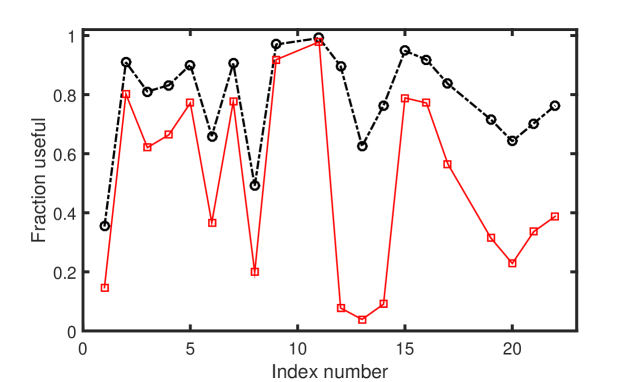
Figure 5: A summary of the standard errors of 20 of the spectral indices (see Table 1 for definitions). The K-b and CaH-1 indices have been excluded, since these poorly calibrated for the later spectral types. Shown are the fractions, across 232 spectra, which have estimated standard errors smaller than 0.1 (points connected by solid lines) or smaller than 0.2 (points connected by broken lines). Some indices are clearly less resistant to noise.

Here $\ell_{n}$ and $\ell_{d}$ are respectively the number of spectral elements in the numerator and denominator intervals, while $F_{n}$ and $F_{d}$ are the fluxes in the numerator and denominator intervals. Information about standard errors for the sample of 232 individual SALT spectra is summarised in Fig. 5. Plotted are the fractions of indices with standard errors smaller than 0.2 (broken line) or smaller than 0.1 (solid line). Judging by this, indices 2-5 (CaH2, CaH3, TiO2, TiO-a), 7 (TiO5), 9 (VO7434), 11 (VO7912), 15 (TiO844) and 16 (CrH-a) are particularly useful for the sample of UCDs dominated by late M to early L objects. Note that with the exception of index 12 (Na8190) this list includes the four indices proposed by Hawley et al. (2002) which are within the SALT spectral range. Cruz et al. (2009) fig. 4 shows 8 alkali-metal indices useful for discriminating gravity effects: of these, Cs-b is outside the spectral range of SALT; the denominator of the K-a index is within the excluded Fraunhofer A wavelength range; K-b is poorly calibrated by the template spectra; and all the remaining indices (Rb-a, Rb-b, Na-a, Na-b, Cs-a) are prone to high noise levels. On the other hand, three of the four molecular gravity indicators in Cruz et al.(2009) fig. 5 (VO-a$\equiv$TIO7434, TiO-b$\equiv$TiO8440 and CrH-a) are in the list of useful indices given above. In what follows indices with estimated standard errors in excess of 0.2 were not taken into account.

3.3 Median index fitting (MIF)

An alternative method using spectral indices, based on a median spectral type, was also used. The approach is designed to limit the impact of spurious classifications supported by few indices. The methodology is as follows:

• Note that for a given index, possible spectral classes are essentially read from the relevant plot in Figs. 1-4, i.e. spectral types are real, rather than integer.

• Since spectral type is typically a multi-valued function of spectral index, several spectral subclasses are usually associated with each index. (For example, spectral types L1.0, L2.8, L5.6 and L7.3 all have TiO4 indices near unity). This clearly leads to ambiguity. At the outset all spectral types implied by each of the spectral indices are collected.

• Possible classifications are narrowed down by rejecting from the list determined in (ii) all types more than three subclasses from the TF classification.

• The median spectral subclass of the remaining candidate types is then selected as the best index-based classification.

In all but 17 cases types derived in this fashion are within 1.5 subclasses of the template value; this level of agreement is better than that obtainable with the index-based methods defined by (2) or (3).

3.4 Classification confidence

It is, of course, desirable to have some indication of the reliability of classifications. It is tempting to use some sort of $\chi^{2}$ procedure to compare the different values of $SS_{1}$ or $SS_{2}$ [in Eqns. (1) or (2)] over different spectral class fits. Formally this could be done using a procedure such as Bartlett’s $\chi^{2}$ test (Bartlett 1937). However, it is well known (e.g. Conover, Johnson & Johnson 1981) that this procedure is sensitive to deviations from Gaussianity – i.e. a significant value of the statistic may simply be due to the fact that fit residuals are non-Gaussian. A simple alternative is to use a permutation procedure. For template fitting, based on (1), it would work as follows:

• Choose a suitable test statistic, e.g.

  $$U_{t}=SS_{1}(t)/\min_{t}SS_{1}(t)\equiv SS_{1}(t)/SS_{1}(t_{0})$$ (5)

  i.e. $t_{0}$ is the index of the best-fitting template, and $t$ the index of a candidate alternative.

• Define the two sets of residuals

  $$e_{0}(\lambda) = F_{S}(\lambda)-\beta_{0}F_{0}(\lambda)$$

  $$e_{t}(\lambda) = F_{S}(\lambda)-\beta_{t}F_{t}(\lambda)$$

  where $F_{0}$ is the best-fitting template, $F_{t}$ the candidate alternative, and the wavelength $\lambda$ takes on all the observed values. In terms of the residuals

  $$U_{t}=\sum_{\lambda}e_{t}(\lambda)/\sum_{\lambda}e_{0}(\lambda)$$ (6)

• Pool the values of $e_{0}$ and $e_{t}$ and randomly divide them into two new sets of values $e_{0}^{\prime}$ and $e_{t}^{\prime}$.

• Calculate the statistic $U_{t}^{\prime}$ as defined in (6), using $e_{0}^{\prime}$ and $e_{t}^{\prime}$.

• Repeat steps (iii) and (iv) many (preferably a few thousand) times, saving the new value of $U_{t}^{\prime}$ for each replication.

• The significance level of $U_{t}$ calculated in (i) is then established by noting its rank in the collection of $U_{t}^{\prime}$.

The method sketched above has the virtue of being completely distribution-free, but the drawback of being time consuming if many observed spectra are processed. A compromise is therefore made: the non-parametric variance comparison test of Fligner & Killeen (1976) is used instead. Limited experimentation suggests that the permutation test, the Fligner & Killeen (1976) procedure, and the more widely used Brown-Forsythe test (Brown & Forsythe 1974) all give comparable results (see also Conover et al. 1981). The acronym “FK” will be used below to refer to the Fligner & Killeen (1976) test.

The question remains as to which significance level to conduct the test at. Testing is unconventional, since the aim is to ascertain which templates (or sets of spectral indices) provide viable alternatives to the best-fitting one. The value adopted was $p=0.1$, i.e. a 10% chance of obtaining such a large variance for the alternative classifications, as compared to the variance associated with the best-fitting template or spectral index set. (Quite similar results are obtained with $p=0.2$). For convenience, the term “confidence set” will be used for the collection of spectral classes which are statistically equivalent (as defined above) to the best-fitting one.

3.5 Comparison of the three classification methods

It comes as no surprise that the confidence sets are smaller for template fitting than for fitting based on spectral indices: the number of points being fit is two orders of magnitude greater in the former case. Although calculation of the spectral indices involves taking averages, the wavelength intervals are relatively narrow, and taking ratios inflates uncertainties. Only 20 of the template fits to the 232 individual SALT spectra have confidence sets larger than 3 subclasses, whereas 102 of the spectral index-based classifications have confidence sets greater than 5 subclasses.

To summarise: the most dependable classification tool is TF, followed by the restricted median of the collection of spectral types (MIF), as derived from the spectral indices. There are very few cases where results from TF and MIF are incompatible, and in those cases the disagreement is marginal, as demonstrated by MIF spectral types being in the confidence sets of the TF classifications. Unrestricted index matching, as described in subsection 3.3, is very inefficient as compared to the other two methods. The reason, alluded to in subsection 3.3, is that spectral type is not a unique function of spectral index for any of the indices in Figs. 1-4. Restricting the part of the multi-valued function to be considered ameliorates this problem. Furthermore, the median of the spectral types from all the indices is more representative of the information content of the set of indices than the mean spectral type.

A few representative examples of templates fitted to SALT spectra can be seen in Fig. 6.

4 SPECTRAL CLASSIFICATION: RESULTS

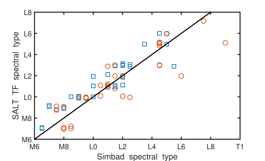
Figure 7: A comparison between literature spectral types extracted from the Simbad database, and those obtained from template fitting (TF) to SALT spectra. The line indicates equal spectral classes. Circles and squares respectively denote literature classification based on infrared and optical spectra. For greater clarity the SALT spectral classes have been jittered by adding Gaussian random numbers with zero mean and a standard deviation of 0.1 subclasses.

There are 73 averaged SALT spectra of 49 objects with spectral classifications provided by the Simbad database; these were used to test performance of our classification software. A graphical comparison between the literature spectral types and those obtained from SALT TF can be seen in Fig. 7. (The SALT spectral types have been randomly offset by small amounts, to avoid many points being coincident). Circles denote optical literature spectra, while squares indicate infrared spectra. Interestingly, there does not seem to be a systematic difference between our classifications and Simbad types based on infrared spectra, although the scatter around the equal-types line is larger for the infrared spectra.

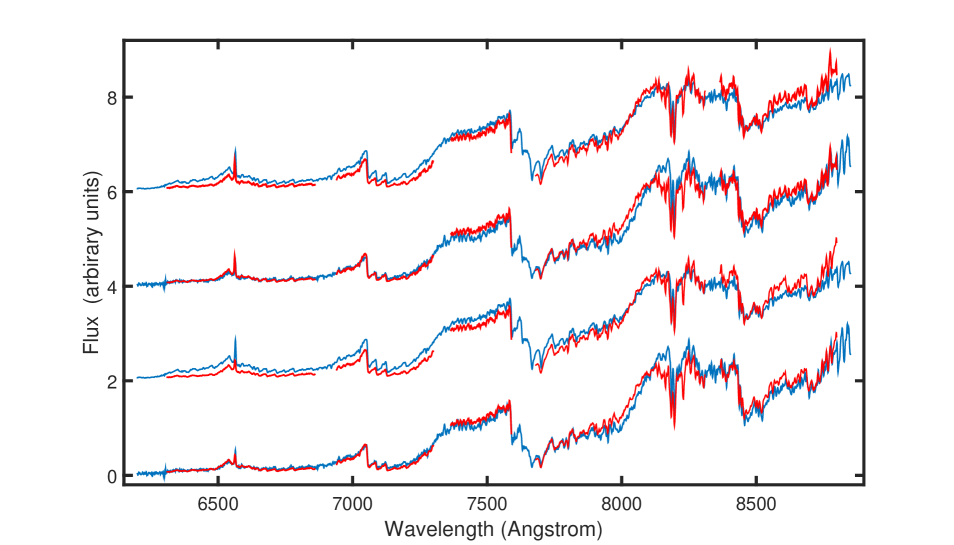
Figure 8: Fits of template spectra to two SALT spectra of 2M 1655-0823 (VB 8). The top two plots show the SALT spectrum obtained on 2014 March 12, with M7 (top) and M9 templates. The bottom two plots show the SALT spectrum from 2014 June 30, also with M7 (top) and M9 templates.

Agreement between TF classifications and those listed in Simbad is generally good, with 88% of types differing by less than 2 spectral subclasses. The figure for MIF classifications is similar – 78%. SALT TF types differ by two or more spectral classes from Simbad classifications for 8 UCDs – see Table 3:
2M 0128-5545 Kendall et al. (2007) assigned a NIR spectral class of L1, but remarked that some spectral indices suggested a type about 2 subclasses later. Martín et al. (2010) also classified the UCD as L1. The template fit to the SALT spectrum suggests an unambiguous L3 type, and this is confirmed by the spectral indices (20 of which were usable).
2M 0223-5815 Cruz et al.(2009) classify this object as L0$\gamma$, meaning “very low gravity L0”. The $p$-value of the FK test statistic is 0.59 for the L1 spectral fit. It may be concluded that the template fit to the SALT spectrum is not unique, and does not markedly contradict the L0 classification in the literature.
2M 0230-0953 Widely different classifications of 2M 0230-0953 have been published by respectively Martín et al. (2010) (optical spectrum, L0) and Marocco et al. (2013) (NIR spectrum, L6). The three individual SALT spectra give classifications consistently in the range L1-L3. We adopt a mean classification of L2.
2M 1523-2347 and 2M 1548-1636 Classifications of L2.5 and L2 were assigned to 2M 1523-2347 and 2M 1548-1636 respectively by Kendall et al. (2007), on the basis of NIR spectra. All SALT spectra give consistent results of L0 for both objects. Given the remarks on NIR typing in the Introduction, the latter classification is recommended.
2M 1655-0823 This is a very well-studied object (current Simbad citation count is 333), better known by the names GJ 644C, LHS 429 and VB 8. Use of the spectrum as an M7 standard appears to date back to Boeshaar & Tyson (1985). There have been some remarks about abnormalities in the spectrum (Dahn, Liebert & Harrington 1986). SALT spectra of 2M 1655-0823 were obtained at two epochs; M7 and M9 templates fitted to these are plotted in Fig. 8. It is immediately apparent that whereas the M7 template fits the strong features in the range 8000-8500 Å quite well, the M9 template fits the continuum blueward of about 7800 Å much better. It is noteworthy that the best classification obtained from fitting spectral indices [Eqn. (2)] is M7, for both spectra. It is cautiously concluded that whereas the spectral indices are those of an M7 dwarf, the shape of the continuum is unusual, and not fitted perfectly by any one standard form.
2M 2252-1730 The T0 classification listed in Simbad is a revision by Schneider et al. (2014), based on a NIR spectral classification, of the spectral type assigned by Reid et al (2006). The latter authors found the object to be a binary with L6$\pm 1$ and T2/3 components. The SALT optical spectral type is comparable with the Reid et al. (2006) NIR classification of the brighter component.
2M 2255-5713 The object is a binary composed of L6 and L8-T1 components (Reid et al. 2008a). Interestingly, both SALT spectra show an even greater excess at shorter wavelengths than that visible in Reid et al. (2008)’s fig. 2. This clearly cannot be ascribed to the fainter companion, but may be due to contamination by a faint background star.

It should be clear from the discussion that there is little reason to doubt the automated classification of the SALT spectra. New proposed classifications for some of the objects are given in the penultimate column of Table 3.

It is perhaps worthwhile to also consider those spectra for which the difference between the TF classification and that extracted from the Simbad database is 1.5 subclasses. Information about the spectra, corresponding to 9 different UCDs, appears in Table 4:
2M 0651-1446 and 2M 1308-4925 The existing classifications of these objects are due to Folkes et al. (2012), based on NIR spectra. Template fitting of 2M 0651-1446 select a spectral type of M9 with M8 a very close second. MIF spectral types are also around M8. A classification of M8.5 seems appropriate. As far as 2M 1308-4925 is concerned, the M7 template fits are considerably better than any competitor, while the indices are consistent with types in the range M7.3-7.4. A classification of M7 is adopted.
2M 0814-4020 There is good agreement between the TF and MIF types derived from the SALT spectra, giving a classification in the range M8-M9. The only published classification, by Gálvez-Ortiz et al. (2014), is M7-M8. The proposed classification is M8.5.
2M 0847-1532 On discovery the object was classified L2 (Cruz et al. 2003), and was listed as an L2 spectral standard by Reid et al.(2008b). The Simbad spectral classification of L1.5 is from a NIR classification by Schneider et al. (2014). As indicated in Table 4, L2-L3 templates fit the data almost equally well, showing compatibility with the previous classifications.
2M 1454-6604 The Simbad classification of L3.5 is taken from Phan-Bao et al. (2008). The most likely classification of the two individual SALT spectra is L5, with L6 distant second choices. A spectral class of L5 is also supported by the MIF.
2M 1520-4422 This UCD has attracted a fair amount of attention. It is a spatially resolvable binary ($\sim 1.2$ arcsec separation). Spectral classifications of L2+L4 (Kendall et al. 2007) and L1.5+L4.5 (Burgasser et al. 2007) have been made, based on NIR spectra. Classification by spectral indices lie in a narrow range of L2.2-L2.3.
2M 1845-6357 This UCD, better known as SCR J1845-6357A, was classified as an M8.5 dwarf by Henry et al. (2004), based on an 8.7 Å resolution optical spectrum. The two $S/N=100$ SALT spectra summarised in Table 3 suggest an alternative classification: although the FK statistic rejects alternative fits, the Brown-Forsythe statistic indicates that the M9 template fits are not much worse than L0. Bearing in mind also the MIFs, an M9.5 classification is proposed.
2M 2224-0158 The Simbad spectral type of L4.5 is from Kirkpatrick et al. (2000). Fits of the L4 and L5 templates are comparable to the best fit (L6), and the MIF type is L6.2. There is enough uncertainty to accommodate the published spectral type.
2M 2308-2722 Templates in the range L1-L3 fit almost equally well, i.e. the classification formally accords with the literature spectral type.

It may be concluded that in general the classifications in this paper are within one subclass of previous classifications. Greater differences can largely be ascribed to uncertainties (as reflected in the confidence sets) or sometimes large differences between optical and NIR classifications. Table 5 lists classifications of the remaining SALT spectra of UCDs with published spectral types: in a few cases slightly different classifications are proposed.

First spectral classifications are provided in Table 6 for 32 UCDs. These were taken from the catalogue of Folkes et al. (2012), who selected UCD candidates near the galactic plane. The authors used a combination of 2MASS NIR photometry, optical photometry extracted from photographic surveys, and proper motion information, to construct their catalogue.

In the majority of cases two SALT spectra obtained in succession have been averaged. In a few cases spectra were obtained at more than one epoch (see the dates in column 2). There is only one object in the Table for which the TF and MIF types differ by more than 1.3 classes, namely 2M 0819-4706. This is one of the seven UCDs for which the confidence set consists of three spectral types, i.e. the fit is more uncertain than most. The spectral index classification agrees with the latest of the three types in the TF confidence set. The mean number of indices used for classification (i.e. with estimated standard errors smaller than 0.2) is 16, and only two classification rely on fewer than 10 indices.

Four of the entries in Table 6 have been marked with asterisks, indicating that the spectra are unusual. Two of these – 2M 0739-4926 and 2M 0811-4319 – have substantially elevated blue continua, while the blue continuum in 2M 0838-3211 is substantially depressed compared to the red part of the spectrum. A blue excess could easily be explained by the presence of a faint background star (which is overwhelmingly more likely to be bluer than the UCD), but a reason for the absence of blue light in 2M 0838-3211 is less obvious. The spectra of 2M 0819-4706 shows contamination by diffuse galactic H II emission.

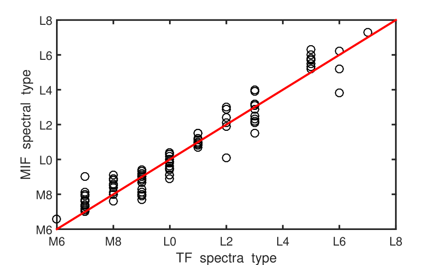
Figure 9: A comparison of spectral types from template fitting (TF) and from the the median of spectral indices (MIF), for all the stars for which SALT spectra were obtained. The line indicates equal spectral classes.

A graphical comparison between TF and MIF spectral classifications is made in Fig. 9, for all the stars in Tables 3-6. The are no global systematic differences between the two classification schemes. There are three objects with classification differences larger than 1.5 subclasses – two of these are known to have unusual spectra, namely 2M 0141-4633 (TF type L2) and 2M 1126-5003 (TF type L6). The former is known to be a young, low gravity UCD (Kirkpatrick et al. 2006, 2008; Cruz et al. 2009) while the latter has an unusual spectrum, ascribed to the presence of condensates in its photosphere (Burgasser et al. 2008). The third discrepant point in Fig. 9 is due to 2M 0819-4706, mentioned in the preceding paragraph.

5 H$\alpha$ EMISSION

Many papers have been published on “activity” in UCDs, the term usually meaning “the presence of H$\alpha$ emission”. A sampling is Schmidt et al. (2007), Reiners & Basri (2008), Berger et al. (2009), Lee et al. (2010), Berger et al (2010), Stelzer et al. (2012), Schmidt et al. (2015), and Pineda et al. (2016). References to other (particularly earlier) work can also be found in these references. Although it is usually assumed that activity is magnetic, accretion is another possibility (e.g. Koen 2008, Scholz et al. 2009).

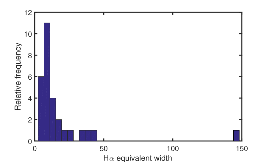
Figure 10: Histogram of the non-zero H$\alpha$ EWs measured from the SALT spectra. Mean values are shown in those cases where objects were observed at multiple epochs.

Out of the 81 UCDs with SALT spectra 28 showed measurable H$\alpha$ emission. Equivalent widths for the individual spectra are listed in the last columns of Tables 3-6, and a histogram of the results is plotted in Fig. 10. Three of the UCDs observed on multiple occasions showed intermittent emission, while emission was either consistently absent or present in the remaining 25 objects observed more than once.

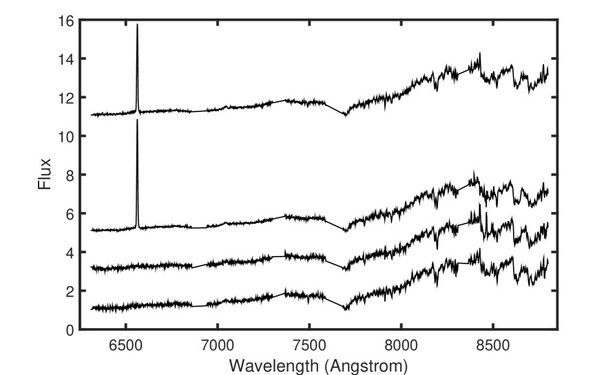
Figure 11: Spectra of 2MASS 1520-4422, showing occasional very strong H$\alpha$ emission. The top two spectra were obtained in succession on 2014 June 22, the bottom two in succession on 2014 August 3.

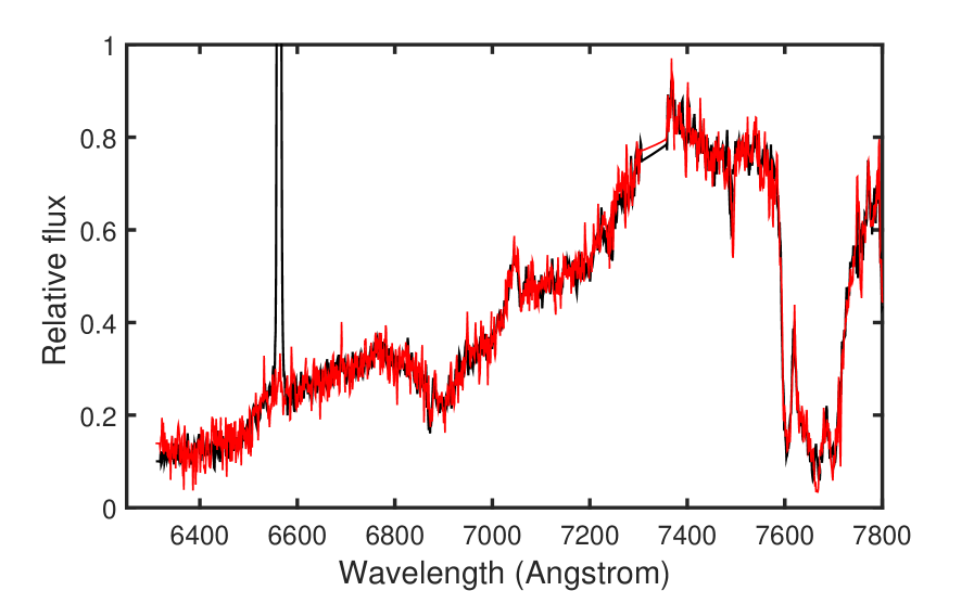
Figure 12: Average of the two 2014 June 22 spectra of 2MASS 1520-4422 (black) and of the two 2014 August 3 spectra (red). Note that the two continuum levels are the same, despite the presence of the strong flare in the earlier spectra.

The binary UCD 2M 1520-4422, responsible for the outlying point in Fig. 10, was observed at two epochs. The two pairs of spectra acquired are plotted in Fig. 11. Remarkable H$\alpha$ emission (EWs of 135 and 157 Å) can be seen in spectra obtained in June 2014. An interesting point is that there is no apparent enhancement of the blue continuum in these earlier spectra, as compared to the later pair (see Fig. 12). This contrasts with e.g. the flaring behaviour observed by Liebert et al. (1999) in the M9.5 object 2MASS J0149090+295613. It is also noteworthy that there is no trace at all of emission in the later spectra: Phan-Bao et al. (2008) also quote an EW for 2M 1520-4433 smaller than 4 Å . Notably, no other emission features aside from H$\alpha$ are present in any of the spectra.

The different responses to flaring seen in the continua of 2M 1520-4422 and 2M 0149+2956 is interesting. Note that 2M 1520-4422 is not unique in showing no continuum enhancement – compare fig. 11 in Schmidt et al. (2007), which shows three spectra of 2MASS J10224821+5825453 (type L1). Although H$\alpha$ emission EWs varied from 24 to 128 Å the continua appear unaffected. It is tempting to think that flares in UCD of spectral types L are not accompanied by continuum increases, while the converse holds for earlier spectral types. However, “white light” flares have also been seen in the L1 dwarf WISEP J190648.47+401106.8 (Gizis et al. 2013) and L0 dwarf SDSS J053341.43+001434.1 (Schmidt et al. 2016). Conditions which determine the presence or absence of increases in continuum emission in L dwarfs clearly deserve more study.

Another point which deserved discussion is that the $J$ magnitudes of the two component of 2M 1520-4422 differ by about 1.15 mag (Burgasser et al. 2007). Given the difference of 2-3 in spectral subclasses (Kendall et al. 2007, Burgasser et al. 2007), the blue flux of the fainter companion could be about an order of magnitude below that of the brighter object. This implies that a blue continuum enhancement due to a flare in the fainter companion may be difficult to detect.

The ratio of H$\alpha$ luminosity $L_{H\alpha}$ to bolometric luminosity $L_{\rm bol}$ is a standard measure of the level of activity. A straightforward way of calculating it is to use the equation

$$L_{H\alpha}/L_{\rm bol}=\chi{\rm EW(H\alpha)}\;.$$

The factor $\chi$, which is a function of spectral class, was introduced by Walkowicz et al. (2004), and is conveniently tabulated for UCDs in Schmidt et al. (2014). The latter paper gives a mean value of $\chi=2.18\times 10^{-6}$ for both L1 and L2 subclasses, leading to $\log~{}(L_{H\alpha}/L_{\rm bol})=-3.53,-3.47$ for the equivalent widths quoted above. The above assumes that the brighter A component of 2M 1520-4422 is responsible for the emission; if it is the later B component (L4-L4.5), $\chi\approx 1.2\times 10^{-6}$ and $\log~{}(L_{H\alpha}/L_{\rm bol})=-3.79,-3.72$.

An alternative activity measure is the ratio of H$\alpha$ and bolometric fluxes (e.g. Schmidt et al. 2007). Burgasser et al. (2007) estimate NIR magnitudes of the A and B components of 2M 1520-4422 as $J=13.55$, $K_{S}=12.27$; $J=14.70$, $K_{S}=13.22$ respectively. Using bolometric corrections for spectral types of L1.5 and L4.5 interpolated in the tables of Schmidt et al. (2014), mean apparent bolometric magnitudes of 15.49 and 16.50 are obtained for the two components. From the relation

$$m_{\rm bol}=-2.5\log F_{\rm bol}-11.48$$

and H$\alpha$ line fluxes of 1.08 and 1.20$\times 10^{-14}$ erg cm^-2 s^-1, $\log(F_{H\alpha}/F_{\rm bol})=-3.18,-3.13$ if the emission is associated with the brighter component, or $\log(F_{H\alpha}/F_{\rm bol})=-2.77,-2.73$ if it originates in the fainter component.

These activity strengths are far in excess of any seen at these spectral types in the substantial sample (181 L dwarfs) discussed by Schmidt et al. (2015) (see their figs. 6 and 7). The only L dwarfs for which comparable activity levels have, to the authors’ knowledge, been reported are 2MASS J1315309-264951 (Gizis 2002, Hall 2002, Burgasser et al. 2011, and references therein) and 2MASS J10224821+5825453 (Schmidt et al. 2007). Spectral classification of 2M 1315-2649 is L5e (indicating sustained, rather than flaring emission). The discovery papers reported H$\alpha$ equivalent widths $\sim 100$ Å and activity measures $\log~{}(L_{H\alpha}/L_{\rm bol})$ in the range -4.1 to -3.9. In the case of 2M 1022+5825 (L1), an H$\alpha$ EW of 128 Å was observed on one occasion, with lower levels of emission on two other nights (Schmidt et al. 2007).

A lesson imparted by the above is that it may be risky to draw conclusions about activity levels from the information currently available: given the remarkable difference between the two sets of spectra in Fig. 10, several visits to any one target may be required to elicit the range of its H$\alpha$ emission.

6 CONCLUSIONS

The primary results of this paper are

• Quantification of the uncertainty in spectral classification, by means of robust variance-comparison statistics, was proposed.

• The full collection of SALT spectra was used to evaluate classification by twenty different spectral indices. Half of these generally have large standard errors; this includes the alkali-metal gravity-sensitive indices.

• An alternative classification method by spectral indices was introduced, namely the median of all spectral types implied by all accurately determined indices.

• There is generally good agreement between the results of template fitting of SALT spectra, and published classifications. In a number of instances revised spectral types have been proposed – typically when fits are unambiguous (one-member confidence sets), with closely similar MIF classifications.

• First spectral classifications of 32 UCD candidates were presented in Table 6. The great majority of classifications are either unambiguous, or of types M8-M9, which often suggests a class of M8.5.

• Measurable H$\alpha$ emission was seen in 28 of the UCDs. For most of the objects observed at multiple epochs the emission is either consistently present, or consistently absent.

• One set of spectra of 2MASS 1520-4422 showed H$\alpha$ flares with equivalent widths in excess of 130 Å. Interestingly, spectra at a different epoch had no sign of even low level emission.

It should be emphasized that although classification based on continuum matching is favoured in this paper, considerable additional information is available from detailed examination of spectral features, as described, for example, by spectral indices. Examples are sensitivity to gravity (Kirkpatrick et al. 2008, Cruz et al. 2009, Martín et al. 2010), metallicity (Lépine, Rich & Shara 2007; Burgasser 2008, West et al. 2011) and the presence of atmospheric condensates (Burgasser et al. 2008).

REFERENCES

Allers K.N., Liu M.C., 2013, ApJ, 772, 79

Berger E., et al., 2009, ApJ, 695, 310

Bartlett M.S., 1937, Proc. Roy. Stat. Soc. A, 160, 268

Bochanski J.J., West A.A., Hawley S.L., Covey K.R., 2007, AJ, 133, 531

Boeshaar P.C.,Tyson J.A., 1985, AJ, 90, 817

Brown M.B., Forsythe A.B., 1974, J. Amer. Stat. Assoc., 69, 364

Buckley D.A.H., Swart G.P., Meiring J.G., 2006, SPIE, 6267, 0Z

Burgasser A.J., 2008, in Van Belle G., (ed), The 14th Cambridge Workshop on Cool Stars, Stellar Systems and the Sun. ASP Conf. Ser., 384, 126 (Astronomical Society of the Pacific).

Burgasser A.J., Looper D.L., Kirkpatrick J.D., Liu M.C., 2007, AJ, 658, 557

Burgasser A.J., Looper D.L., Kirkpatrick J.D., Cruz K.L., Swift B.J., 2008, ApJ, 674, 451

Burgh E.B., Nordsieck K.H., Kobulnicky H.A., Williams T.B., O’Donoghue D., Smith M.P., Percival J.W., 2003, SPIE, 4841, 1463

Conover W.J., Johnson M.E., Johnson M.M., 1981, Technometrics, 23, 351

Crawford S.M., et al., 2010, SPIE, 7737, 25

Cruz K.L., Reid I.N., Liebert J., Kirkpatrick J.D., Lowrance P.J., 2003, AJ, 126, 2421

Cruz K.L., Kirkpatrick J.D., Burgasser A.J., 2009, AJ, 137, 3345

Dahn C.C., Liebert J., Harrington R.S., 1986, AJ, 91, 621

Fligner M.A., Killeen T.J., 1976, J. Amer. Stat. Assoc., 71, 210

Folkes S.L., et al., 2012, MNRAS, 427, 3280

Gálvez-Ortiz M.C., et al., 2014, MNRAS, 439, 3890

Gizis J.E., 2002, ApJ, 575, 484

Gizis J.E., Burgasser A.J., Berger E., Williams P.K.G., Vrba F.J., Cruz K.L., Metchev S., 2013, ApJ, 779, 172

Hall P.B., 2002, ApJ, 564, L89

Hambly N.C., et al., 2001, MNRAS,326, 1279

Hawley S.L., et al., 2002, AJ,123, 3409

Henry T.J., Subasavage J.P., Brown M.A., Beaulieu T.D., Jao W.-C., 2004, AJ, 128, 2460

Kendall T.R., Jones H.R.A., Pinfield D.J., Pokorny R.S., Folkes S., Weights D., Jenkins J.S., Mauron N., 2007, MNRAS, 374, 445

Kirkpatrick J.D., 2008, in Gray R.O., Corbally C.J., Stellar Spectral Classification. Princeton University Press, Princeton, p. 354

Kirkpatrick J.D., et al., 1999, ApJ, 519, 802

Kirkpatrick J.D., et al., 2000, AJ, 120, 447

Kirkpatrick J.D., Barman T.S., Burgasser A.J., McGovern M.R., McLean I.S., Tinney C.G., Lowrance P.J., 2006, ApJ, 639, 1120

Kirkpatrick J.D., et al., 2008, ApJ, 689, 1295

Kobulnicky H.A., Nordsieck K.H., Burgh E.B., Smith M.P., Percival J.W., Williams T.B., O’Donoghue D., 2003, SPIE, 4841, 1634

Koen C., 2008, MNRAS, 389, 949

Lee K.-G., Berger E., Knapp G.R., 2010, ApJ, 708, 1482

Lépine S., Rich R.M., Shara M., ApJ, 669, 1235

Liebert J., Kirkpatrick J.D., Reid I.N., Fisher M.D., 1999, ApJ, 519, 345

Lodieu N., Scholz R.-D., McCaughrean M.J., Ibata R., Irwin M., Zinnecker H., 2005, A&A, 440, 1061

Luhman K.L., Stauffer J.R., Muench A.A., Rieke G.H., Lada E.A., Bouvier J., Lada C.J., 2003, ApJ, 593, 1093

Marocco F., et al., 2013, AJ, 146, 161

Martín E.L., et al., 2010, A&A 517, A53

Metodieva Y., Antonova A., Golev V., Dimitrov D., García-Älvarez D., Doyle J.G., 2015, MNRAS, 446, 3878

O’Donoghue D., et al., 2006, MNRAS, 372, 151

Phan-Bao N., et al., 2008, MNRAS, 383, 831

Pineda J.S.,Hallinan G.,Kirkpatrick J.D., Cotter G., Kao M.M., Mooley K., 2016, ApJ, in press

Reid I.N., Hawley S.L., Gizis J.E., 1995, AJ, 110, 1838

Reid I.N., Lewitus E., Burgasser A.J., Cruz K.L., 2006, ApJ, 639, 1114

Reid I.N., Cruz K.L., Burgasser A.J., Liu M.C., 2008a, AJ,135, 580

Reid I.N., Cruz K.L., Kirkpatrick J.D., Allen P.R., Mungall F., Liebert J., Lowrance P., Sweet A., 2008b, AJ,136, 1290

Reiners A., Basri G., 2008, ApJ, 684, 1309

Schmidt S.J., Cruz K.L., Bongiorno B.J., Liebert J., Reid I.N., 2007, AJ, 133, 2258

Schmidt S.J., West A.A., Bochanski J.J., Hawley S.L., Kielty C., 2014, PASP, 126, 642

Schmidt S.J., Hawley S.L., West A.A., Bochanski J.J., Davenport J.R.A., Ge J., Schneider D.P., 2015, AJ, 149, 158

Schmidt S.J., et al., 2016, ApJ, 828, L22

Schneider A.C., Cushing M.C., Kirkpatrick J.D., Mace G.N., Gelino C.R., Faherty J.K., Fajardo-Acosta S., Sheppard S.S., 2014, AJ, 147, 34

Scholz A., Xu X., Jayawardhana R., Wood K.,Eislöffel J., Quinn C., MNRAS, 398, 873

Skrutskie M.F., et al., 2006, AJ, 131, 1163

Stelzer B., et al., 2012, A&A, 537, A94

van Dokkum P.G., 2001, PASP, 113, 1420

Walkowicz L.M., Hawley S.L., West A.A., 2004, PASP, 116, 1105

West A.A., Bochanski J.J., Bowler B.P., Dotter A., Johnson J.A., Lépine S., Rojas-Ayala B., Schweitzer A., 2011, in Johns-Krull C.M., Browning M.K., West A.A., (eds), The 16th Cambridge Workshop on Cool Stars, Stellar Systems and the Sun. ASP Conf. Ser., 448, 531 (Astronomical Society of the Pacific).

Williams P.K.G., Cook B.A., Berger E., 2014, ApJ, 785:9

Table 1.   Log of SALT-RSS observations.

Name	Date	Exposure
(2MASS J)	(mm/dd/yyyy)	(s)
10484281$+$0111580	04/16/2014	2$\times$600
14540797$-$6604476	04/16/2014	2$\times$600
15074769$-$1627386	04/19/2014	2$\times$600
19165762$+$0509021	05/03/2014	800
16553529$-$0823401	05/03/2014	600
17502484$-$0016151	05/11/2014	2$\times$600
07123786$-$6155528	05/12/2014	2$\times$600
08472872$-$1532372	05/12/2014	2$\times$600
10101480$-$0406499	05/12/2014	2$\times$600
17453466$-$1640538	05/12/2014	2$\times$600
22134491$-$2136079	05/12/2014	2$\times$600
12212770$+$0257198	06/12/2014	2$\times$600
12281523$-$1547342	06/12/2014	2$\times$600
00325584$-$4405058	06/12/2014	2$\times$600
17502484$-$0016151	06/29/2014	600, 700
17453466$-$1640538	06/29/2014	2$\times$600
16553529$-$0823401	06/30/2014	600
19165762$+$0509021	06/30/2014	800
15074769$-$1627386	07/07/2014	2$\times$600
14540797$-$6604476	07/09/2014	2$\times$600
22134491$-$2136079	07/09/2014	2$\times$600
23225299$-$6151275	07/09/2014	2$\times$600
22244381$-$0158521	07/09/2014	2$\times$600
00332386$-$1521309	07/12/2014	2$\times$600
01282664$-$5545343	07/12/2014	2$\times$600
17054834$-$0516462	07/13/2014	2$\times$600
13054019$-$2541059	07/13/2014	2$\times$600
23225299$-$6151275	07/14/2014	2$\times$600
01415823$-$4633574	07/14/2014	2$\times$600
02235464$-$5815067	07/14/2014	600
00242463$-$0158201	07/31/2014	600
08593060$-$6605084	12/12/2014	3$\times$600
00145575$-$4844171	12/15/2014	3$\times$600
07522427$-$3925410	01/01/2015	2$\times$600
06512977$-$1446150	01/02/2015	2$\times$600
12342370$-$5104354	01/02/2015	2$\times$600
08115730$-$4319238	01/04/2015	2$\times$600
09420802$-$3758418	01/04/2015	2$\times$600
11032796$-$5933001	01/04/2015	2$\times$600

Table 1.   continued.

Name	Date	Exposure
(2MASS J)	(mm/dd/yyyy)	(s)
09474621$-$3810043	01/05/2015	2$\times$600
10192447$-$2707171	01/05/2015	2$\times$600
10503781$-$4517010	01/05/2015	2$\times$600
12405746$-$6549554	01/05/2015	2$\times$600
08383219$-$3211406	01/06/2015	2$\times$600
08274661$-$1619256	01/06/2015	2$\times$470
11263991$-$5003550	01/06/2015	2$\times$600
11312945$-$6446032	01/06/2015	2$\times$600
11224462$-$6533161	01/06/2015	2$\times$600
07595440$-$2117123	01/07/2015	2$\times$600
06482289$-$2916280	01/15/2015	2$\times$600
08193434$-$4706133	01/30/2015	2$\times$600
08143545$-$4020492	02/01/2015	2$\times$600
11301046$-$5759419	02/04/2015	2$\times$600
07410404$-$0359495	02/07/2015	600
13080663$-$4925505	03/02/2015	2$\times$600
07561708$-$0715512	03/07/2015	2$\times$600
08173001$-$6155158	03/27/2015	2$\times$600
06465202$-$3244011	03/28/2015	2$\times$600
07293904$-$2608578	03/28/2015	2$\times$600
17502484$-$0016151	03/28/2015	2$\times$600
06164933$-$1411434	03/29/2015	2$\times$600
12065011$-$3937261	03/29/2015	2$\times$600
07313276$-$2841575	03/29/2015	2$\times$600
10565008$-$6122042	03/30/2015	2$\times$600
17373472$-$3446108	03/31/2015	2$\times$600
17054834$-$0516462	03/31/2015	2$\times$600
13201384$-$4842117	03/31/2015	2$\times$600
07390794$-$4926533	04/24/2015	2$\times$600
18422444$-$1358138	04/30/2015	550, 600
14263345$-$5229166	04/30/2015	600
16445570$-$2618333	04/30/2015	2$\times$600
16445570$-$2618333	05/02/2015	2$\times$600
06482289$-$2916280	05/03/2015	2$\times$600
07293904$-$2608578	05/03/2015	2$\times$600
11224462$-$6533161	05/03/2015	2$\times$600

Table 1.   continued.

Name	Date	Exposure
(2MASS J)	(mm/dd/yyyy)	(s)
14334194$-$5148037	05/04/2015	2$\times$600
08193434$-$4706133	05/24/2015	3$\times$600
10192447$-$2707171	05/25/2015	2$\times$600
17502484$-$0016151	06/18/2015	2$\times$600
15200224$-$4422419	06/22/2015	2$\times$600
00065794$-$6436542	07/01/2015	600
21501324$-$6610366	07/01/2015	2$\times$600
00311925$-$3840356	07/02/2015	2$\times$600
17502484$-$0016151	07/03/2015	2$\times$600
15200224$-$4422419	07/03/2015	2$\times$600
15485834$-$1636018	07/06/2015	2$\times$600
00065794$-$6436542	07/06/2015	2$\times$1200
17072529$-$0138093	07/13/2015	2$\times$600
20131084$-$1242452	07/13/2015	600
21501324$-$6610366	07/15/2015	2$\times$600
20131084$-$1242452	07/19/2015	600
13080663$-$4925505	07/22/2015	229, 600
12191303$-$5021426	07/28/2015	2$\times$600
14324269$-$5534247	07/28/2015	2$\times$600
22551861$-$5713056	07/28/2015	2$\times$600
00311925$-$3840356	07/28/2015	2$\times$560
17072529$-$0138093	08/01/2015	2$\times$600
15485834$-$1636018	08/01/2015	2$\times$600
01165283$-$6455570	08/01/2015	2$\times$600
17054834$-$0516462	08/02/2015	2$\times$600
01165283$-$6455570	08/06/2015	2$\times$600
22521073$-$1730134	08/06/2015	2$\times$600
23081134$-$2722001	08/06/2015	2$\times$600
15410782$-$6026051	08/12/2015	3$\times$600
18052143$-$0733179	08/12/2015	2$\times$600
14324269$-$5534247	08/14/2015	2$\times$600
16445570$-$2618333	08/14/2015	2$\times$600
01333248$-$6314415	08/14/2015	2$\times$600
14334194$-$5148037	08/15/2015	2$\times$600
19265883$-$0844206	08/15/2015	2$\times$530
14263345$-$5229166	08/16/2015	2$\times$600
15230657$-$2347526	08/16/2015	2$\times$600

Table 1.   continued.

Name	Date	Exposure
(2MASS J)	(mm/dd/yyyy)	(s)
16533670$-$3855165	08/16/2015	2$\times$600
16532340$-$6424077	08/17/2015	2$\times$600
18473965$-$1856577	08/17/2015	3$\times$600
18002648$+$0134566	08/21/2015	2$\times$600
17275293$-$6227029	08/24/2015	2$\times$600
23211254$-$1326282	08/24/2015	500, 600
15410782$-$6026051	09/08/2015	350, 2$\times$600
00145575$-$4844171	10/01/2015	2$\times$600
01333248$-$6314415	10/01/2015	2$\times$600
07293904$-$2608578	10/01/2015	2$\times$600
18450541$-$6357475	10/02/2015	2$\times$600
06164933$-$1411434	10/03/2015	2$\times$600
02304498$-$0953050	10/03/2015	3$\times$600
07230144$-$1616209	10/05/2015	2$\times$600
06400355$-$1449104	10/06/2015	2$\times$600
06512977$-$1446150	10/06/2015	2$\times$600

Table 2.   Spectral indices considered for use in classifications: the wavelength intervals (in Å ) used for calculation of the numerator and denominator of the flux ratios are listed. In some cases the inverses of indices defined in the literature were used, in order that the ranges of numerical values be similar across all 22 indices.

No.	Name	Numerator	Denominator		No.	Name	Numerator	Denominator
1	TiO1	6718-6723	6703-6708		10	K-b	7550-7570	7690-7710
2	CaH2	6814-6846	7042-7046		11	VO7912	7900-7980	8400-8420
3	CaH3	6960-6990	7042-7046		12	Na8190	8140-8165	8173-8210
4	TiO2	7058-7061	7043 7046		13	Na-a	8153-8163	8178-8188
5	TiO-a	7058-7073	7033-7048		14	Na-b	8153-8163	8190-8200
6	TiO3	7092-7097	7042-7046		15	TiO8440	8440-8470	8400-8420
7	TiO5	7126-7135	7042-7046		16	CrH-a	8580-8600	8621-8641
8	TiO4	7130-7135	7042-7046		17	FeH-a	8660-8680	8700-8720
9	VO7434	7430-7470	7550-7570
18	CaH1	6380-6390	6345-6355, 6410-6420
19	Rb-a	7795-7805	7775-7785, 7815-7825
20	Rb-b	7943-7953	7923-7933, 7963-7973
21	VO-b	7960-8000	7860-7880, 8080-8100
22	Cs-a	8516-8526	8496-8506, 8536-8547

Table 3.   Instances where SALT TF classifications differ by two or more subclasses from types given in the Simbad database. In some cases revised spectral classifications are proposed (penultimate column). Non-zero H$\alpha$ emission equivalent widths are listed in the last column.

Name	Simbad	TF	Confidence Set		MIF	Final	EW(H$\alpha$)
							(Å)
2MASS J01282664-5545343	L1	L3	L3		L2.9	L3
2MASS J02235464-5815067	L0	L2	L1 - L2		L2.1	L1.5
2MASS J02304498-0953050	L6	L2	L1 - L3		L2.9	L2
2MASS J15230657-2347526	L2.5	L0	L0		M9.8	L0
2MASS J15485834-1636018	L2	L0	L0		M9.9	L0
	L2	L0	L0		L0.0
2MASS J16553529-0823401	M7	M9	M7 - M9		M7.9		9
	M7	M9	M8 - M9		M7.9		6
2MASS J22521073-1730134	T0	L5	L5		L5.8	L5
2MASS J22551861-5713056	L5.5	L3	L3		L3.9

Table 4.   Instances where SALT TF classifications differ by 1.5 subclasses from types given in the Simbad database. In some cases revised spectral classifications are proposed (penultimate column). Non-zero H$\alpha$ emission equivalent widths are listed in the last column.

Name	Simbad	TF	Confidence Set		MIF	Final	EW(H$\alpha$)
							(Å)
2MASS J06512977-1446150	M7.5	M9	M8 - M9		M8.3	M8.5	25
	M7.5	M9	M8 - M9		M8.0		10
2MASS J08143545-4020492	M7-M8	M9	M8 - M9		M8.7	M8.5
2MASS J08472872-1532372	L1.5	L3	L2 - L3		L3.2
2MASS J13080663-4925505	M8.5	M7	M7		M7.4	M7	5
	M8.5	M7	M7		M7.3		4
2MASS J14540797-6604476	L3.5	L5	L5		L5.5	L5
2MASS J15200224-4422419	L4.5	L3	L1 - L3		L2.3		146
	L4.5	L3	L1 - L3		L2.2
2MASS J18450541-6357475	M8.5	L0	L0		M9.1	M9.5	5
2MASS J22244381-0158521	L4.5	L6	L4 - L6		L6.2
2MASS J23081134-2722001	L1.5	L3	L1 - L3		L3.2		10

Table 5.   UCDs for which SALT TF classifications differ by less than 1.5 subclasses from types given in the Simbad database. In some cases revised spectral classifications are proposed (penultimate column). Non-zero H$\alpha$ emission equivalent widths are listed in the last column.

Name	Simbad	TF	Confidence Set		MIF	Final	EW(H$\alpha$)
							(Å)
2MASS J00065794-6436542	M9	L0	M8 - L0		M9.4	M9.5
2MASS J00145575-4844171	L2.5	L3	L3		L4.0	L3
	L2.5	L3	L1 - L3		L2.5
2MASS J00242463-0158201	M9.5	L0	L0		L0.4	L0
2MASS J00311925-3840356	L2	L1	L1 - L3		L1.5
	L2	L3	L3		L2.1
2MASS J00325584-4405058	L0	L0	L0 - L2		L0.3
2MASS J01165283-6455570	L1	L1	L0 - L1		L0.8
2MASS J01333248-6314415	M8	M7	M7		M7.3	M7	3.5
	M8	M7	M7		M7.2		5
2MASS J01415823-4633574	L2	L2	L1 - L2		L0.1
2MASS J07123786-6155528	L1	L2	L2 - L3		L3.0	L2	15
2MASS J08274661-1619256	M8	M9	M8 - M9		M8.8	M8.5
2MASS J10192447-2707171	M9.5	L0	L0		M9.5	L0	5
	M9.5	L0	L0		L0.0		9
2MASS J10484281+0111580	L1	L1	L1		L0.9
2MASS J10503781-4517010	M9	L0	L0		M9.1	L0	10
2MASS J11263991-5003550	L5	L6	L3 - L6		L3.8
2MASS J12065011-3937261	L2	L2	L2 - L3		L2.4	L2.5
2MASS J12212770+0257198	L0.5	L0	L0		L0.2	L0	2.5
2MASS J12281523-1547342	L5	L5	L5 - L6		L6.3	L5.5
2MASS J13054019-2541059	L2	L3	L3		L3.1	L3
	L2	L3	L3		L3.2	L3
2MASS J14263345-5229166	M8	M7	M7		M7.1	M7
	M8	M7	M7		M7.4
2MASS J14334194-5148037	M6.5	M7	M7		M7.1	M7	20
	M6.5	M7	M7		M7.3		16
2MASS J15074769-1627386	L5	L5	L5		L5.7
	L5	L6	L5 - L6		L5.2
2MASS J17054834-0516462	L1	L1	L1		L1.2
	L1	L1	L1		L1.5
	L1	L1	L1		L1.0
2MASS J17072529-0138093	L0.5	L1	L1		L1.0	L1
2MASS J17453466-1640538	L1.5	L1	L1		L0.9	L1
	L1.5	L1	L1		L1.1

Table 5.   continued.

Name	Simbad	TF	Confidence Set		MIF	Final	EW(H$\alpha$)
							(Å)
2MASS J17502484-0016151	L4.5	L5	L5		L5.3	L5
	L4.5	L5	L5		L5.2
	L4.5	L5	L5		L5.7
	L4.5	L5	L5		L6.0
	L4.5	L5	L5		L5.7
2MASS J18002648+0134566	L7.5	L7	L7 - L8		L7.3
2MASS J19165762+0509021	M8	M9	M8 - M9		M8.9	M8.5	5
	M8	M9	M8 - M9		M9.0		8
2MASS J20131084-1242452	L1.5	L1	L1 - L2		L0.8
	L1.5	L2	L1 - L3		L1.9
2MASS J21501324-6610366	M9	L0	M8 - L0		M9.5
	M9	L0	M8 - L0		M9.5
2MASS J22134491-2136079	L0	L1	L0 - L1		L0.7	L0.5
2MASS J23211254-1326282	L1	L1	L1 - L2		L1.0
2MASS J23225299-6151275	L2	L3	L2 - L4		L1.5	L2.5
	L2	L2	L1 - L3		L2.9

Table 6.   New classifications. TF and MIF types are in columns 3 and 5, with final classifications in column 7. Column 2 gives the date of observation and column 6 the number of spectral indices used to derive the MIF type. Non-zero H$\alpha$ emission equivalent widths are listed in the last column. See the text for remarks about objects marked with an asterisk.

Name	Date	TF	Confidence Set		MIF	No. indices	Final	EW(H$\alpha$)
	(DD MM YY)							(Å)
2MASS J06164933-1411434	29 03 15	M8	M8 - L0		M8.6	14	M9-L0
	03 10 15	L0	L0		L0.3	11
2MASS J06400355-1449104	06 10 15	M8	M8 - M9		M8.1	19	M8.5	11
2MASS J06465202-3244011	28 03 15	M8	M8 - M9		M8.8	20	M8.5	45
2MASS J06482289-2916280	15 01 15	M8	M8 - M9		M8.0	15	M8
	03 05 15	M8	M8		M9.1	19		15
2MASS J07230144-1616209	05 10 15	L1	L1		L1.0	20	L1
2MASS J07293904-2608578	28 03 15	M9	M9		M8.7	18	M9	10
	03 05 15	L0	M8 - L0		M9.6	7
	01 10 15	M9	M9		M9.4	19		6
2MASS J07313276-2841575	29 03 15	M9	M8 - M9		M9.1	17	M8.5
2MASS J07390794-4926533*	24 04 15	L1	L1		L0.8	20	L1

Table 6   continued.

Name	Date	TF	Confidence Set		MIF	No. indices	Final	EW(H$\alpha$)
	(DD MM YY)							(Å)
2MASS J07410404-0359495	07 02 15	L0	L0		M9.9	20	L0
2MASS J07522427-3925410	01 01 15	M9	M9		M9.0	16	M9	20
2MASS J07561708-0715512	07 03 15	M8	M8 - M9		M8.9	15	M8.5
2MASS J07595440-2117123	07 01 15	M9	M8 - M9		M8.1	9	M8.5	40
2MASS J08115730-4319238*	04 01 15	M7	M7		M8.1	19	M7	10
2MASS J08193434-4706133*	30 01 15	M7	M7		M7.9	15	M7
	24 05 15	M7	M7		M9.0	12
2MASS J08383219-3211406*	06 01 15	M7	M7		M7.6	18	M7
2MASS J08593060-6605084	12 12 14	M9	M8 - M9		M9.0	17	M9	25
2MASS J09420802-3758418	04 01 15	M9	M8 - M9		M8.9	13	M8.5
2MASS J09474621-3810043	05 01 15	M8	M8		M8.0	18	M8
2MASS J11224462-6533161	06 01 15	M8	M8 - M9		M8.9	13	M8.5
	03 05 15	M8	M8 - M9		M8.4	19
2MASS J11312945-6446032	06 01 15	M9	M8 - M9		M9.2	12	M8.5
2MASS J12191303-5021426	28 07 15	M9	M9		M8.1	19	M9	33
2MASS J12342370-5104354	02 01 15	M9	M8 - M9		M8.0	15	M9	15
2MASS J12405746-6549554	05 01 15	M7	M7		M7.7	17	M7
2MASS J13201384-4842117	31 03 15	M9	M8 - M9		M9.0	15	M9	10
2MASS J14324269-5534247	28 07 15	M9	M8 - M9		M9.3	18	M8.5
	14 08 15	M8	M8 - M9		M8.5	10
2MASS J15410782-6026051	12 08 15	M6	M6 - M7		M6.6	19	M7	4
	08 09 15	M7	M7		M7.6	15		5
2MASS J16445570-2618333	30 04 15	M8	M8 - M9		M7.6	18	M8.5	7
	02 05 15	M9	M8 - M9		M7.7	19		6
	14 08 15	M7	M7		M7.6	18		7
2MASS J16533670-3855165	16 08 15	M7	M7 - M9		M7.6	20	M8	9
2MASS J17275293-6227029	24 08 15	L0	M8 - L0		M8.9	17	L0
2MASS J18422444-1358138	30 04 15	M7	M7		M7.3	19	M7	8
2MASS J18473965-1856577	17 08 15	M7	M7		M7.0	17	M7
2MASS J19265883-0844206	15 08 15	M7	M7		M8.0	15	M7	15