Analysis of scalar dissipation in terms of
vorticity geometry in isotropic turbulence

Abstract

The mechanisms promoting scalar dissipation through scalar gradient production are scrutinized in terms of vorticity alignment with respect to strain principal axes. For that purpose, a stochastic Lagrangian model for the velocity gradient tensor and the scalar gradient vector is used. The model results show that the major part of scalar dissipation occurs for stretched vorticity, namely when the vorticity vector aligns with the extensional and intermediate strain eigenvectors. More specifically, it appears that the mean scalar dissipation is well represented by the sample defined by alignment with the extensional strain, while the most intense scalar dissipation is promoted by the set of events for which vorticity aligns with the intermediate strain. This difference is explained by rather subtle mechanisms involving the statistics of both the strain intensities and the scalar gradient alignment resulting from these special alignments of vorticity. The analysis allowing for the local flow structure confirms the latter scenario for both the strain- and rotation-dominated events. However, despite the prevailing role of strain in promoting scalar dissipation, the difference in the level of scalar dissipation when vorticity aligns with either the extensional or the intermediate strain mostly arises from rotation-dominated events.

1 Introduction

The finest level at which micromixing in fluid flows can be investigated is determined by the local gradient of a scalar. The gradient indeed rules molecular diffusion, but also gives a precise insight into the small-scale structure of scalar fields and mixing patterns. Actually, it is the mean dissipation rate of the energy of scalar fluctuations, $D\langle\bm{G}^{2}\rangle$, the so-called scalar dissipation – with $D$ the molecular diffusivity and $\bm{G}$ the scalar gradient –, which reveals the efficiency of micromixing. Modelling small-scale mixing in process and chemical engineering [1] or in combustion flow computation [2] thus needs to understand the very mechanisms of scalar gradient production. On the basic level, the study of the scalar gradient is relevant to the general problem of vector transport in fluid flows [3] including the kinematics of vectors defining material lines or surfaces [4], the vorticity vector properties [5, 6], the dynamics of the vorticity gradient in two-dimensional flows [7] as well as the production of the magnetic field by the motion of a conducting fluid [8].

A number of studies have tackled the connection of the detailed features of the scalar gradient and of the scalar dissipation with the properties of the flow field determined by the local velocity gradients [9, 10, 11, 12, 13, 14, 15, 16, 17, 18, 19, 20]. Clearly, in scalar gradient production, strain – through its intensity, persistence and the respective alignments of scalar gradient and principal axes – is the chief mechanism, while vorticity, at least its magnitude, is immaterial. Because of the tight interaction between strain and vorticity [5, 21], however, vorticity properties are likely to be indirectly involved. In fact, the role of strain in the vicinity of vorticity structures has early been established [9, 10, 11]. Models based on stretched vortices [22] have also been shown to reproduce the physics of scalar transport and mixing in turbulent flows. More recently the influence of vortical structures on mixing has been clearly shown [23].

The present work, too, has to do with the relationship between mixing properties and the local features of the flow field. The production of scalar dissipation, and thus the mechanisms of micromixing, are probed through the kinematic features of the scalar gradient in terms of vorticity geometry. Since vorticity alignments arise from the dynamics of the velocity field and are closely connected to the inner, detailed structure of turbulent flows [5, 6, 24], alignment of vorticity with respect to strain principal axes is especially considered.

This article reports an extension of the findings presented in reference [25]. The stochastic Lagrangian model used in the study is described in Section 2 and its ability to predict statistics conditioned on vorticity alignments is checked in Section 3. Making use of the model results, the scrutiny of scalar dissipation in terms of vorticity geometry, including the analysis based on local flow structure, is achieved in Section 4. Conclusion is drawn in Section 5.

2 Stochastic Lagrangian model for the velocity and scalar gradients

2.1 Modelled equations

The model for the velocity gradient tensor has been derived by Chevillard and Meneveau [26] and has been shown to predict the essential geometric properties and anomalous scalings of incompressible, isotropic turbulence [26, 27]. Starting from an Eulerian-Lagrangian change of variables and using the Recent Fluid Deformation Approximation the modelled equation for the velocity gradient tensor, ${\bm A}$, is derived as

$$d{\bm A}=\left(-{\bm A}^{2}+\frac{Tr({\bm A}^{2})}{Tr({\bm C}_{\tau_{\eta}}^{-1})}{\bm C}_{\tau_{\eta}}^{-1}-\frac{Tr({\bm C}_{\tau_{\eta}}^{-1})}{3T}{\bm A}\right)dt+{\left(\frac{2}{T}\right)}^{1/2}d{\bm W}$$ (1)

in which $T$ is the integral time scale and ${\bm C}_{\tau_{\eta}}$ is a model for the Cauchy-Green tensor, ${\bm C}_{\tau_{\eta}}=\exp({\tau_{\eta}{\bm A}})\exp({\tau_{\eta}{\bm A}^{T}})$, where $\tau_{\eta}$ is the Kolmogorov time scale. Forcing is ensured by the increment of a tensorial Wiener process, $d{\bm W}=dt^{1/2}{\bm\zeta}$, where ${\bm\zeta}$ is a tensorial, Gaussian delta-correlated noise with $\langle\zeta_{ij}\rangle=0$ and $\langle\zeta_{ij}\zeta_{kl}\rangle=2\delta_{ik}\delta_{jl}-1/2\delta_{ij}\delta_{kl}-1/2\delta_{il}\delta_{jk}$.

This model has been extended to the gradient of a passive scalar [28]. The modelled equation for the scalar gradient is written

$$d{\bm G}=-\left({\bm A}^{T}{\bm G}+\frac{Tr({\bm C}_{\tau_{\eta}}^{-1})}{3T_{\theta}}{\bm G}\right)dt+{\left(\frac{2}{T_{\theta}}\right)}^{1/2}d{\bm W}_{\bm G}$$ (2)

where $T_{\theta}$ is the scalar integral time scale and $d{\bm W}_{\bm G}=dt^{1/2}{\bm\xi}$ is the increment of a Wiener process where ${\bm\xi}$ is a vectorial, Gaussian noise such that $\langle\xi_{i}\rangle=0$ and $\langle\xi_{i}\xi_{j}\rangle=\delta_{ij}$.

In the model represented by Eqs. (1) and (2) stretching is exactly taken into account, while models are devised for the pressure Hessian – second term of Eq. (1) –, viscous effects – third term of Eq. (1) – and molecular diffusion – second term of Eq. (2). Meneveau has given a detailed discussion on this class of stochastic Lagrangian models [29].

2.2 Numerical solution

Time scales are normalised by the integral time scale ($T=1$). As in reference [28] the Kolmogorov time scale and the scalar integral time scale are respectively prescribed as $\tau_{\eta}=0.1$ – which corresponds to a Taylor microscale Reynolds number, ${\rm Re}_{\lambda}$, close to 150 [27] – and $T_{\theta}=0.4$.

Equations (1) and (2) are solved using a second-order predictor-corrector scheme [30]. The calculation is run for $2\times 10^{5}T$ with time step $10^{-2}$ and the statistics of the velocity and scalar gradients are derived from their respective stationary time signals.

3 Predictions of statistical features conditioned on vorticity properties

The model retrieves the main features of the scalar gradient statistics and kinematics [28], namely the non-gaussian properties of the scalar gradient components, the probability density functions (p.d.f.’s) of the production of scalar gradient norm, the statistical alignments with respect to strain principal axes and vorticity as well as more subtle features already underlined in two-dimensional turbulence [31] such as the existence of special preferential alignments. It has also been shown to reproduce the statistics of the scalar gradient in rotating turbulence [32]. This Lagrangian approach has been used to model the evolution of the turbulent magnetic field as well [33]. Additional assessment of the model in connection with the present study relates to statistics conditioned on vorticity alignments. The latter are taken from the direct numerical simulations (DNS) by Tsinober et al. [34] and comparisons with the model predictions are made in Figs. 1 - 3.

The strain eigenvalues are denoted by $\lambda_{i}$ and the corresponding eigenvectors by $\bm{e}_{i}$; the $\lambda_{i}$’s are such that $\lambda_{3}<\lambda_{2}<\lambda_{1}$ with $\lambda_{1}+\lambda_{2}+\lambda_{3}=0$ and $\bm{e}_{1}$, $\bm{e}_{2}$ and $\bm{e}_{3}$ define, respectively, the extensional, intermediate and compressional strain principal axes. Figure 1 displays the normalised average of the intermediate strain eigenvalue conditioned on the alignment of vorticity, $\bm{\omega}$, with respect to the intermediate strain eigenvector and shows that the increase of $\lambda_{2}$ with $|\cos(\bm{\omega},\bm{e}_{2})|$ is reasonably predicted by the model for the whole field as well as for small vorticity.

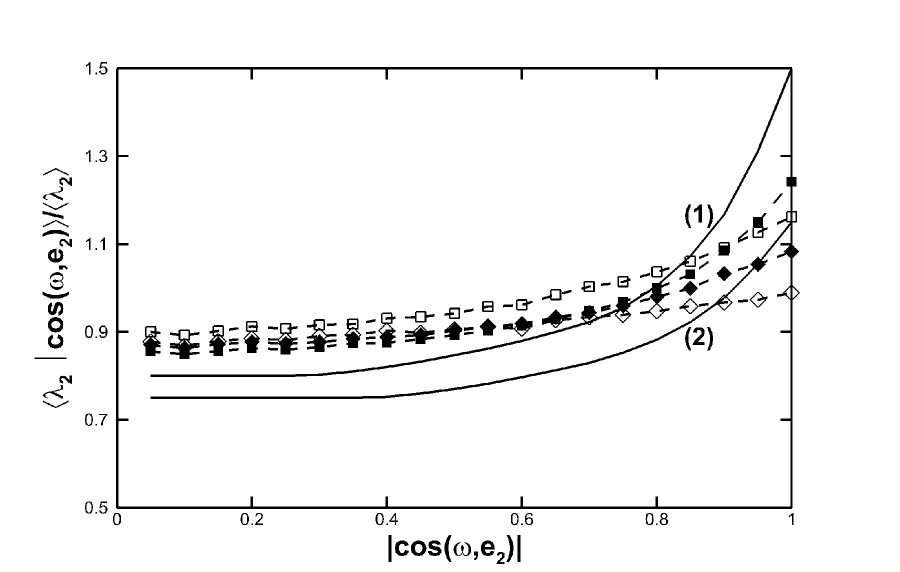
Figure 1: Normalised mean intermediate strain eigenvalue conditioned on the alignment of vorticity with the intermediate strain eigenvector; solid lines: DNS of Tsinober et al. [34]; symbols: model results; (1) and squares: whole field; (2) and diamonds: $\bm{\omega}^{2}<\langle\bm{\omega}^{2}\rangle$; full symbols: ${\rm Re}_{\lambda}\simeq 150$; open symbols: ${\rm Re}_{\lambda}\simeq 75$.

Figure 2 relates to enstrophy production. The model overpredicts the production rate of enstrophy for the strongest alignments between vorticity and the intermediate eigenvector, but displays the right trend for both the whole field and small vorticity, namely the rise of the enstrophy production rate as the alignment gets tighter.

The differences between model predictions and DNS data shown in Figs. 1 and 2 are not explained by a Reynolds number dependence. In fact, Tsinober et al. [34] suggest that their DNS results – although they were derived at ${\rm Re}_{\lambda}\simeq 85$ – are likely to be almost Reynolds-number independent. The model results, displayed for ${\rm Re}_{\lambda}\simeq$ 150 and 75, are consistent with this surmise.

In agreement with the numerical simulations of Tsinober et al. [34] – see their Fig. 11 –, the model also correctly predicts the normalised mean enstrophy production terms conditioned on the alignment between vorticty and the extensional strain eigenvector (Fig. 3).

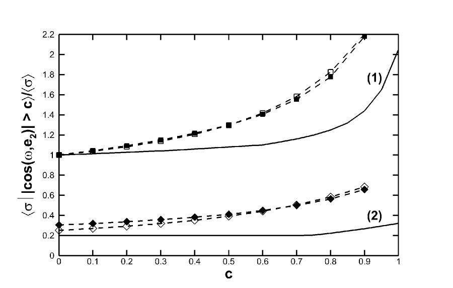
Figure 2: Mean production rate of enstrophy conditioned on strong alignment of vorticity with the intermediate strain eigenvector; $\sigma=\bm{\omega}^{2}[\lambda_{1}\cos^{2}(\bm{\omega},\bm{e}_{1})+\lambda_{2}\cos^{2}(\bm{\omega},\bm{e}_{2})+\lambda_{3}\cos^{2}(\bm{\omega},\bm{e}_{3})]$; solid lines: DNS of Tsinober et al. [34]; symbols: model results; (1) and squares: whole field; (2) and diamonds: $\bm{\omega}^{2}<\langle\bm{\omega}^{2}\rangle$; full symbols: ${\rm Re}_{\lambda}\simeq 150$; open symbols: ${\rm Re}_{\lambda}\simeq 75$.

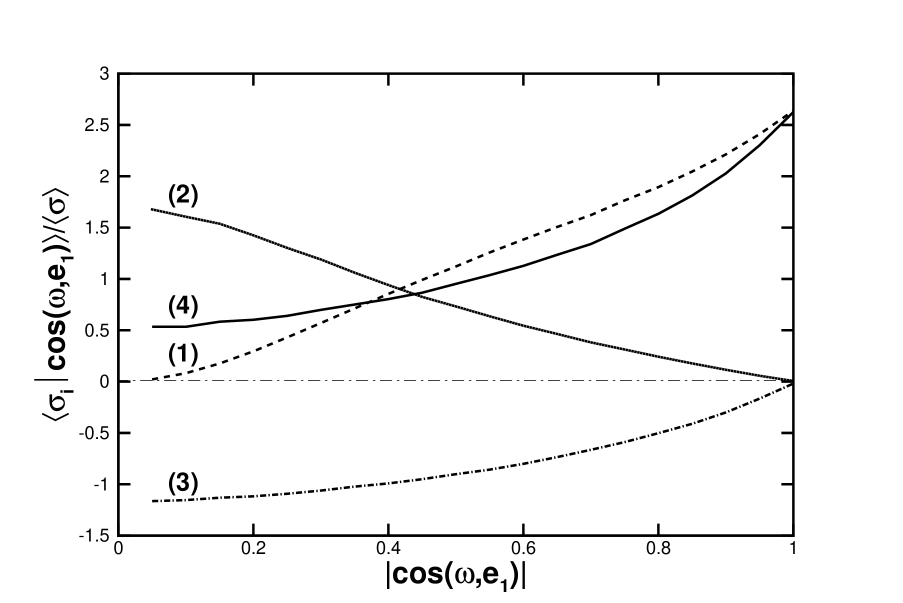
Figure 3: Normalised mean enstrophy production terms conditioned on the alignment of vorticity with the extensional strain eigenvector; (1): average of $\sigma_{1}=\bm{\omega}^{2}\lambda_{1}\cos^{2}(\bm{\omega},\bm{e}_{1})$; (2): average of $\sigma_{2}=\bm{\omega}^{2}\lambda_{2}\cos^{2}(\bm{\omega},\bm{e}_{2})$; (3): average $\sigma_{3}=\bm{\omega}^{2}\lambda_{3}\cos^{2}(\bm{\omega},\bm{e}_{3})$; (4): average of $\sigma=\sigma_{1}+\sigma_{2}+\sigma_{3}$; the figure compares well with Fig. 11 of Tsinober et al. [34].

4 Analysis of scalar dissipation conditioned on vorticity geometry

4.1 Production of scalar gradient vs. vorticity alignments

As scalar dissipation is in direct proportion to the square of the scalar gradient norm, production mechanisms of scalar gradient reveal the way in which it is promoted by the flow field. Using the model, we specifically focus on the case of significant alignment of vorticity with the strain principal axes. The latter is defined by $|\cos(\bm{\omega},\bm{e}_{i})|\geq c$ where $c$ is a threshold spanning the range 0.7 to 0.99 and alignment of vorticity with a strain eigenvector, $\bm{e}_{i}$, is denoted by $\bm{\omega}//\bm{e}_{i}$. The major part – 92% – of the results corresponds to vorticity making an angle smaller than $46^{\circ}$ ($|\cos(\bm{\omega},\bm{e}_{i})|\geq 0.7$) with one of the strain eigenvectors; more precisely, 22% for $i=1$, 55% for $i=2$ and 15% for $i=3$. Vorticity aligning with $\bm{e}_{2}$ is mostly stretched; the intermediate eigenvalue, $\lambda_{2}$, is positive in more than $80\%$ of the $\bm{\omega}//\bm{e}_{2}$-events – 83% for $c=0.7$, 86% for $c=0.99$.

Figure 4 clearly shows the dependence of scalar gradient production on vorticity alignments. The averages of the scalar gradient norm, $\bm{G}^{2}$, and of its production term, $-G_{\alpha}S_{\alpha\beta}G_{\beta}$ (where $\bm{S}$ is the strain tensor), conditioned on $|\cos(\bm{\omega},\bm{e}_{i})|\geq c$ display the same trend: their largest values correspond to strong alignment of vorticity with $\bm{e}_{2}$, while mean values conditioned on alignment with $\bm{e}_{1}$ are closer to the unconditioned averaged values. Alignment of vorticity with the compressional eigenvector, $\bm{e}_{3}$, corresponds to the smallest production. These results thus suggest that the most intense scalar dissipation occurs for $\bm{\omega}//\bm{e}_{2}$, while the mean scalar dissipation is rather well represented by the set of events for which $\bm{\omega}//\bm{e}_{1}$.

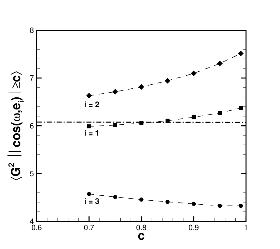
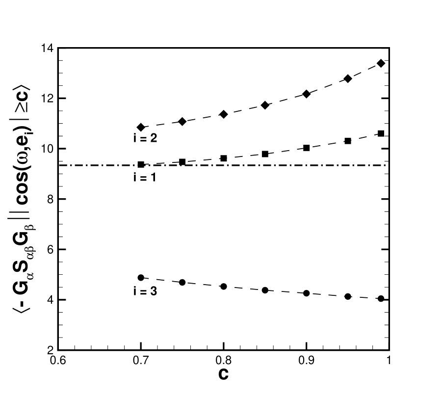
Figure 4: Mean square of scalar gradient norm (a) and production term (b) conditioned on vorticity alignments with respect to the strain eigenvectors, ${\bm e}_{i}$; $i=1$: extensional, $i=2$: intermediate, $i=3$: compressional; dash-dotted line: unconditioned average.

As shown in Fig. 5, when vorticity aligns with a strain eigenvector the intermediate strain causes destruction of the scalar gradient, and the compressional and the extensional strains, as expected, essentially cause production and destruction, respectively. In addition, the differences in scalar gradient production resulting from the vorticity alignments stem from rather subtle mechanisms. From Fig. 5 it is clear that both the weakest production and destruction occur for $\bm{\omega}//\bm{e}_{3}$. Production by the compressional strain as well as destruction by the extensional strain are the largest for $\bm{\omega}//\bm{e}_{2}$, while in this latter case destruction by the intermediate strain coincides with its unconditioned value. For $\bm{\omega}//\bm{e}_{1}$, production by the compressional strain is close to the unconditioned mean value, destruction by the extensional strain is weak and destruction by the intermediate strain is the largest.

These results are supported by the p.d.f’s of $\bm{G}^{2}$ and of the production term $-G_{\alpha}S_{\alpha\beta}G_{\beta}$ (Fig. 6) conditioned on vorticity alignments. In particular, it is clear that extreme values of $\bm{G}^{2}$ are the most probable when $\bm{\omega}//\bm{e}_{2}$. It also appears that both the largest destruction and production of the scalar gradient occur in this case.

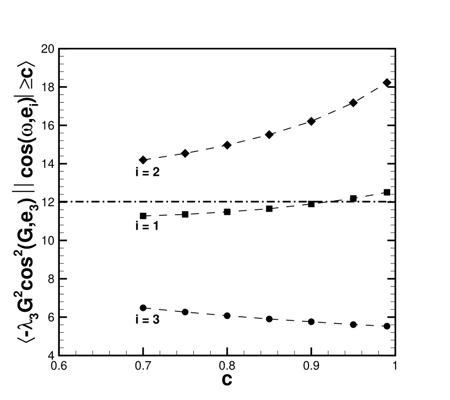
Figure 5: Individual production terms of the mean square of scalar gradient norm conditioned on vorticity alignments with respect to the strain eigenvectors, ${\bm e}_{i}$; (a) production by the extensional strain; (b) by the intermediate strain; (c) by the compressional strain; dash-dotted line: unconditioned average.

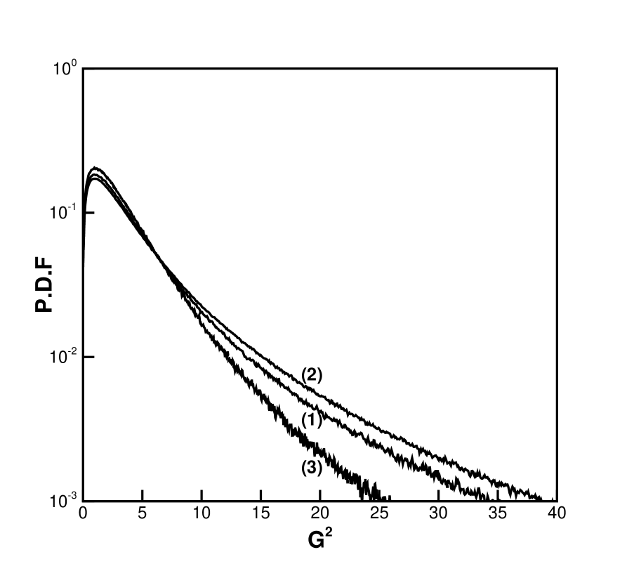
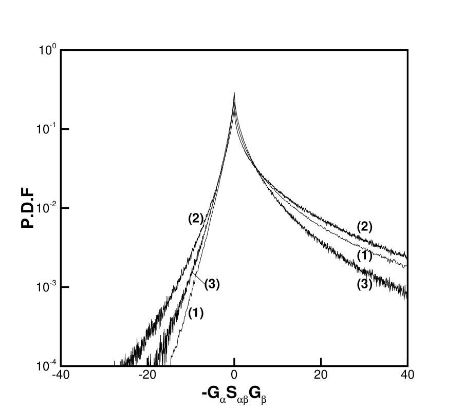
Figure 6: P.d.f’s of (a): $\bm{G}^{2}$ and (b): production term, $-G_{\alpha}S_{\alpha\beta}G_{\beta}$, conditioned on vorticity alignments defined as $|\cos(\bm{\omega},\bm{e}_{i})|\geq 0.8$; (1): $\bm{\omega}//\bm{e}_{1}$; (2): $\bm{\omega}//\bm{e}_{2}$; (3): $\bm{\omega}//\bm{e}_{3}$.

4.2 Analysis of the production mechanisms

The above picture is explained by both the respective intensities of the strain components and the alignments of the scalar gradient with respect to the strain principal axes (Figs. 7 and 8).

When $\bm{\omega}//\bm{e}_{3}$ the scalar gradient alignment with both $\bm{e}_{1}$ and $\bm{e}_{2}$ is rather good, but the weak values of the intensities of the extensional and the intermediate strain result in a weak destruction. However, a small compressional strain intensity together with a poor alignment of the scalar gradient with $\bm{e}_{3}$ also bring about a weak production.

With regard to the difference in scalar gradient production when $\bm{\omega}//\bm{e}_{1}$ or $\bm{\omega}//\bm{e}_{2}$: the extensional strain eigenvalue is the largest and alignment of the scalar gradient with $\bm{e}_{1}$ is the best for $\bm{\omega}//\bm{e}_{2}$ which explains the largest destruction in this case; however, for $\bm{\omega}//\bm{e}_{2}$, the compressional strain eigenvalue is the largest and alignment of $\bm{G}$ with $\bm{e}_{3}$ is slightly better which makes production larger when $\bm{\omega}//\bm{e}_{2}$ than when $\bm{\omega}//\bm{e}_{1}$; furthermore, because the difference in the statistics of the intermediate strain eigenvalue between cases $\bm{\omega}//\bm{e}_{1}$ and $\bm{\omega}//\bm{e}_{2}$ is small and $\bm{G}$ aligns better with $\bm{e}_{2}$ for $\bm{\omega}//\bm{e}_{1}$, destruction by the intermediate strain is larger when $\bm{\omega}//\bm{e}_{1}$. Better alignment of $\bm{G}$ with $\bm{e}_{1}$ for $\bm{\omega}//\bm{e}_{2}$ – and with $\bm{e}_{2}$ for $\bm{\omega}//\bm{e}_{1}$ – results from the trend of the scalar gradient and vorticity to be normal to each other [18, 19] which is predicted by the model [28]. In addition, greater absolute values of the $\langle\lambda_{i}\rangle$’s for $\bm{\omega}//\bm{e}_{2}$ are consistent with the fact that moderate and strong production of strain occurs when vorticity strongly aligns with the intermediate strain eigenvector and is rather misaligned with respect to the extensional strain [21]. It has also been shown [6, 35] that strong alignment of vorticity with $\bm{e}_{2}$ is correlated with large strain intensity. The model reproduces the latter property as shown in Fig. 9 which compares rather well with Fig. 9(d) of reference [6].

To summarize, this analysis suggests that the budget of scalar gradient production resulting in a more intense scalar dissipation for $\bm{\omega}//\bm{e}_{2}$ than for $\bm{\omega}//\bm{e}_{1}$ is explained by the following mechanisms: both extensional strain intensity and scalar gradient alignment explain the difference in the destruction of scalar gradient by the extensional strain, while alignment of the scalar gradient is the main mechanism resulting in a difference in destruction by the intermediate strain; and the difference in the production by compressional strain is to be essentially put down to the compressional strain intensity.

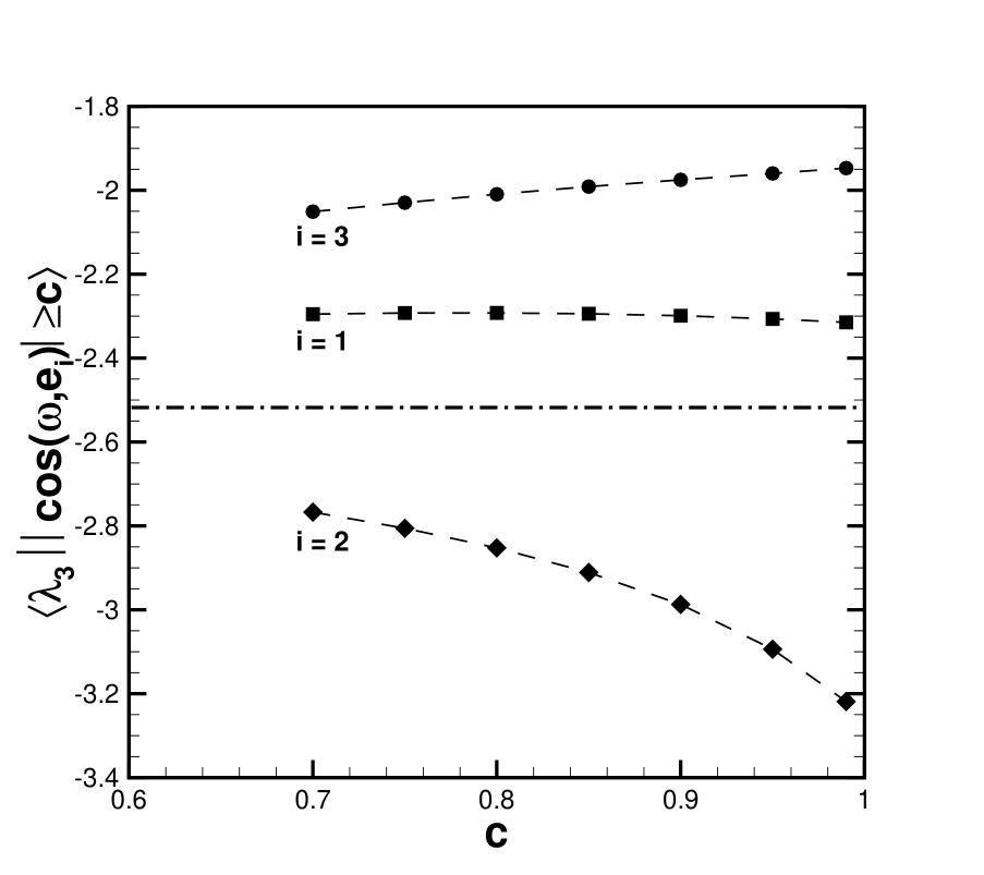
Figure 7: Mean strain eigenvalues conditioned on vorticity alignments with respect to the strain eigenvectors, ${\bm e}_{i}$; (a) extensional strain eigenvalue; (b) intermediate strain eigenvalue; (c) compressional strain eigenvalue; dash-dotted line: unconditioned average.

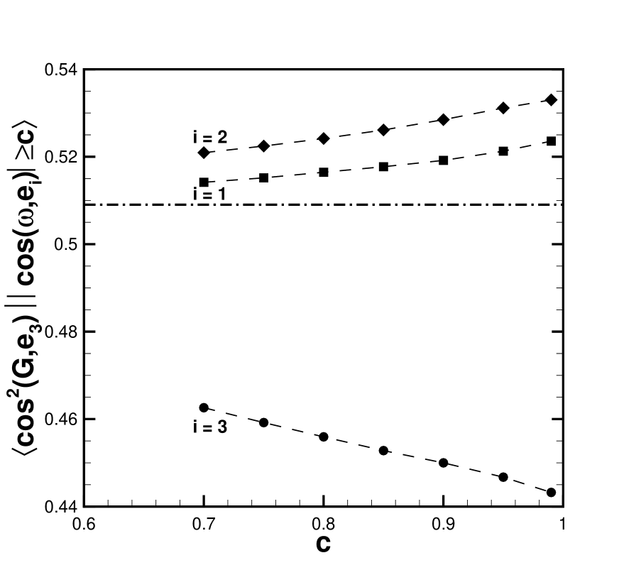
Figure 8: Mean square of director cosines of scalar gradient conditioned on vorticity alignments with respect to the strain eigenvectors, ${\bm e}_{i}$; angle with respect to (a) the extensional strain eigenvector, (b) the intermediate strain eigenvector and (c) the compressional strain eigenvector; dash-dotted line: unconditioned average.

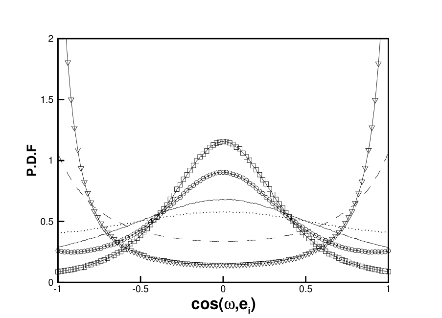
Figure 9: P.d.f’s of vorticity alignments conditioned on strain intensity, $S={(S_{\alpha\beta}S_{\beta\alpha})}^{1/2}$; lines are for $S^{2}<\langle S^{2}\rangle$; dotted: $i=1$, dashed: $i=2$, solid: $i=3$; symbols are for $S^{2}>\langle S^{2}\rangle$; circles: $i=1$, gradients: $i=2$, squares: $i=3$; the figure compares well with Fig. 9(d) of reference [6].

4.3 Analysis in terms of local flow structure

Strain persistence was originally defined in two-dimensional flows [31, 36]. It can be extended to the three-dimensional case [28, 37] when vorticity is closely aligned with a strain eigenvector and used to check whether the flow is locally strain- or rotation-dominated. The strain persistence parameters are computed for $|\cos(\bm{\omega},\bm{e}_{i})|\geq 0.99$ $(i=1,2,3)$ and are respectively given by: $r_{1}=-\omega^{\prime}_{1}/(\lambda_{2}-\lambda_{3})$, $r_{2}=\omega^{\prime}_{2}/(\lambda_{1}-\lambda_{3})$ and $r_{3}=\omega^{\prime}_{3}/(\lambda_{1}-\lambda_{2})$ with $\omega^{\prime}_{i}=\hat{\omega}_{i}-\Omega_{i}$; the $\Omega_{i}$’s are the components of the rotation rate of strain principal axes computed as: $\Omega_{1}=-2\hat{\Pi}_{23}/(\lambda_{2}-\lambda_{3})$, $\Omega_{2}=2\hat{\Pi}_{13}/(\lambda_{1}-\lambda_{3})$ and $\Omega_{3}=-2\hat{\Pi}_{12}/(\lambda_{1}-\lambda_{2})$ where the $\Pi_{ij}$’s are the components of the pressure Hessian tensor, $\Pi_{ij}=(1/\rho)\partial^{2}p/\partial x_{i}\partial x_{j}$ – with $\rho$ and $p$ standing for density and pressure, respectively – modelled as shown in Section 2.1. Hatted quantities indicate components in the strain basis. Prevailing strain is defined by $r_{i}^{2}<1$, while $r_{i}^{2}>1$ indicates prevailing rotation. By including the rotation rate of strain principal axes in addition to vorticity, strain persistence considers the effective rotation rate and was shown to give a better estimate of local stirring properties than criteria just allowing for vorticity [31].

The mechanisms of scalar gradient production can be analysed in terms of prevailing strain vs. prevailing rotation from Table 4.3. Within the text conditioned mean values such as $\langle\bm{G}^{2}|\bm{\omega}//\bm{e}_{i};r_{i}\rangle$ are denoted by $\langle\bm{G}^{2}\rangle_{c}$.

Averaged quantities relevant to scalar gradient production conditioned on vorticity alignment ($|\cos(\bm{\omega},\bm{e}_{i})|\geq 0.99$) and strain persistence parameters, $r_{i}$; $r_{i}^{2}<1$: prevailing strain; $r_{i}^{2}>1$: prevailing rotation; bold numbers represent the unconditioned mean values. strain persistence $r_{1}^{2}<1$ $r_{1}^{2}>1$ $r_{2}^{2}<1$ $r_{2}^{2}>1$ $r_{3}^{2}<1$ $r_{3}^{2}>1$ % in each $\bm{\omega}//\bm{e}_{i}$-sample 38% 62% 49% 51% 9.0% 91% $\langle\bm{G}^{2}|\bm{\omega}//\bm{e}_{i};r_{i}\rangle$ 7.95 5.39 8.22 6.85 4.89 4.27 $\bm{5.15}$ $\langle\lambda_{1}|\bm{\omega}//\bm{e}_{i};r_{i}\rangle$ 1.87 1.55 2.58 2.52 1.94 1.67 $\bm{1.98}$ $\langle\lambda_{2}|\bm{\omega}//\bm{e}_{i};r_{i}\rangle$ 0.979 0.424 0.822 0.523 0.00269 0.278 $\bm{0.534}$ $\langle\lambda_{3}|\bm{\omega}//\bm{e}_{i};r_{i}\rangle$ $-2.86$ $-1.98$ $-3.40$ $-3.04$ $-1.94$ $-1.95$ $\bm{-2.52}$ $\langle\cos^{2}(\bm{G},\bm{e}_{1})|\bm{\omega}//\bm{e}_{i};r_{i}\rangle$ 0.186 0.220 0.236 0.281 0.225 0.253 $\bm{0.239}$ $\langle\cos^{2}(\bm{G},\bm{e}_{2})|\bm{\omega}//\bm{e}_{i};r_{i}\rangle$ 0.229 0.296 0.201 0.215 0.295 0.307 $\bm{0.252}$ $\langle\cos^{2}(\bm{G},\bm{e}_{3})|\bm{\omega}//\bm{e}_{i};r_{i}\rangle$ 0.585 0.485 0.563 0.505 0.480 0.440 $\bm{0.509}$ $\langle-\lambda_{1}\bm{G}^{2}\cos^{2}(\bm{G},\bm{e}_{1})|\bm{\omega}//\bm{e}_{i};r_{i}\rangle$ $-1.22$ $-1.07$ $-4.08$ $-4.70$ $-1.35$ $-1.33$ $\bm{-2.21}$ $\langle-\lambda_{2}\bm{G}^{2}\cos^{2}(\bm{G},\bm{e}_{2})|\bm{\omega}//\bm{e}_{i};r_{i}\rangle$ $-1.06$ $-0.608$ $-0.555$ $-0.337$ $0.103$ $-0.174$ $\bm{-0.444}$ $\langle-\lambda_{3}\bm{G}^{2}\cos^{2}(\bm{G},\bm{e}_{3})|\bm{\omega}//\bm{e}_{i};r_{i}\rangle$ 19.7 8.04 22.0 14.7 7.01 5.38 $\bm{12.0}$ net production 17.4 6.36 17.4 9.66 5.76 3.88 $\bm{9.35}$

In the $\bm{\omega}//\bm{e}_{2}$-sample strain is as frequent as rotation, while the $\bm{\omega}//\bm{e}_{1}$-sample is slightly rotation-dominated which is consistent with a larger scalar dissipation for $\bm{\omega}//\bm{e}_{2}$ than for $\bm{\omega}//\bm{e}_{1}$. This result also suggests that strain is statistically more persistent when vorticity aligns with the intermediate strain eigenvector and may explain the slightly better alignment with the compressional strain direction in this case (Fig. 8). The $\bm{\omega}//\bm{e}_{3}$ sample, by contrast, is found to be strongly rotation-dominated; in these compressed-vorticity events small compressional strain intensity together with a poor alignment of the scalar gradient with $\bm{e}_{3}$ result in low levels of production for both prevailing strain and rotation.

As expected, the largest values of $\langle\bm{G}^{2}\rangle_{c}$ as well as the largest production are found for $\bm{\omega}//\bm{e}_{1}$ and $\bm{\omega}//\bm{e}_{2}$. In agreement with previous studies [18, 19], production mainly results from prevailing-strain events. However, $\langle\bm{G}^{2}\rangle_{c}$ is significant for prevailing rotation as it takes values greater than the unconditioned average for both $\bm{\omega}//\bm{e}_{1}$ and $\bm{\omega}//\bm{e}_{2}$. In addition, the difference between $\bm{\omega}//\bm{e}_{1}$ and $\bm{\omega}//\bm{e}_{2}$ clearly arises from the rotation-dominated events; the difference in $\langle\bm{G}^{2}\rangle_{c}$ is indeed 3.4% for $r_{1}^{2}<1$ and $r_{2}^{2}<1$ – respectively, 7.95 and 8.22 –, while it reaches 27% for $r_{1}^{2}>1$ and $r_{2}^{2}>1$ – respectively, 5.39 and 6.85. For $\bm{\omega}//\bm{e}_{3}$, $\langle\bm{G}^{2}\rangle_{c}$ is smaller than its unconditioned value for both prevailing strain and rotation.

The net production confirms the role of rotation events in the difference between cases $\bm{\omega}//\bm{e}_{1}$ and $\bm{\omega}//\bm{e}_{2}$: the same amount, 17.4, is found for prevailing strain, while for prevailing rotation the net production is equal to 6.36 and 9.66, respectively, namely a difference as large as 52%. As the differences in total destruction by the extensional and the intermediate strains are of the same order for both prevailing strain and prevailing rotation, the large difference in net production for prevailing rotation is mainly explained by production resulting from the compressional strain: 12% for prevailing strain – 19.7 and 22.0 for $\bm{\omega}//\bm{e}_{1}$ and $\bm{\omega}//\bm{e}_{2}$, respectively – and 83% for prevailing rotation – 8.04 and 14.7, respectively. It is also worth noting that production for prevailing rotation when $\bm{\omega}//\bm{e}_{2}$ is not insignificant since both production by the compressional strain – 14.7 – and the net production – 9.66 – are greater than the corresponding unconditioned values, 12.0 and 9.35, respectively.

The mechanisms put forward in Section 4.1 to explain the difference in scalar gradient production between $\bm{\omega}//\bm{e}_{1}$ and $\bm{\omega}//\bm{e}_{2}$ are emphasized by prevailing rotation. The mean values of the extensional and compressional strains, $\lambda_{1}$ and $\lambda_{2}$, are greater when $\bm{\omega}//\bm{e}_{2}$ than when $\bm{\omega}//\bm{e}_{1}$ for both prevailing strain and rotation, but the difference is larger for prevailing rotation: for $\langle\lambda_{1}\rangle_{c}$ the difference is 38% for prevailing strain – respectively, 1.87 and 2.58 – and 63% for prevailing rotation – respectively 1.55 and 2.52; for $\langle\lambda_{3}\rangle_{c}$ these differences are respectively 19% and 54%. Although the difference in the alignment of $\bm{G}$ with respect to $\bm{e}_{1}$ is almost the same for prevailing strain and prevailing rotation – 27% and 28% –, the difference in the alignment with $\bm{e}_{2}$ is larger for prevailing rotation – 14% and 38%.

5 Conclusion

Scalar dissipation has been analysed through scalar gradient production using a stochastic Lagrangian model for the velocity and the scalar gradients which reproduces the essential dynamic and kinematic properties of isotropic turbulence. The study was specifically focused on the connection between vorticity geometry and scalar dissipation, and thus small-scale mixing.

The model results show that scalar dissipation is mainly found when vorticity is stretched. More precisely, for vorticity aligning with the extensional strain, scalar dissipation is close to its unconditioned mean value, while the most intense scalar dissipation – and therefore the most efficient small-scale mixing – occurs for vorticity aligning with the intermediate strain. Scalar dissipation is significantly lower when vorticity is compressed.

The difference in scalar dissipation when vorticity aligns with either the extensional – $\bm{\omega}//\bm{e}_{1}$ – or the intermediate strain – $\bm{\omega}//\bm{e}_{2}$ – is to be put down to the interplay of mechanisms involving the strain intensities and the alignment of the scalar gradient with respect to the strain principal axes. In brief, for $\bm{\omega}//\bm{e}_{2}$ both a larger extensional strain intensity and a better alignment of the the scalar gradient with the extensional strain result in a larger destruction of the scalar gradient norm than when $\bm{\omega}//\bm{e}_{1}$; however, this effect is exceeded by production caused by compression, essentially through a larger compressional strain intensity; in addition, when $\bm{\omega}//\bm{e}_{2}$ it is mainly the misalignment of the scalar gradient with $\bm{e}_{2}$ that causes a lesser destruction by the intermediate strain. For vorticity aligning with the compressional strain direction – $\bm{\omega}//\bm{e}_{3}$ –, weak production of scalar gradient results from both small intensity of the compressional strain and misalignment between the scalar gradient and $\bm{e}_{3}$.

Finally, the latter mechanisms, and especially those explaining the difference in scalar gradient production between $\bm{\omega}//\bm{e}_{1}$ and $\bm{\omega}//\bm{e}_{2}$, are retrieved in the analysis in terms of local flow structure. Although scalar gradient production mostly stems from prevailing-strain events, it appears that this difference is the largest in rotation-dominated events, especially with regard to the extensional and compressional strain intensities.

References

- [1] J. Bałdyga and R. Pohorecki, Turbulent micromixing in turbulent reactors – a review, Chem. Eng. J. 58 (1995), pp. 183–195.
- [2] R.W. Bilger, Some aspects of scalar dissipation, Flow, Turbulence and Combust. 72 (2004), pp. 93–114.
- [3] P.G. Saffman, On the fine-scale structure of vector fields convected by a turbulent fluid, J. Fluid Mech. 16 (1963), pp. 545–572.
- [4] S.S. Girimaji and S.B. Pope, Material-element deformation in isotropic turbulence, J. Fluid Mech. 220 (1990), pp. 427–458.
- [5] K.K. Nomura and G.K. Post, The structure and dynamics of vorticity and rate of strain in incompressible homogeneous turbulence, J. Fluid Mech. 377 (1998), pp. 65–97.
- [6] B. Lüthi, A. Tsinober, and W. Kinzelbach, Lagrangian measurements of vorticity dynamics in turbulent flows, J. Fluid Mech. 528 (2005), pp. 87–118.
- [7] T. Dubos and A. Babiano, Comparing the two-dimensional cascades of vorticity and a passive scalar, J. Fluid Mech. 492 (2003), pp. 131–145.
- [8] B. Favier and P.J. Bushby, Small-scale dynamo action in rotating compressible convection, J. Fluid Mech. 690 (2012), pp. 262–287.
- [9] R.M. Kerr, Higher-order derivative correlations and the alignment of small-scale structures in isotropic numerical turbulence, J. Fluid Mech. 153 (1985), pp. 31–58.
- [10] W.T. Ashurst, A.R. Kerstein, R.M. Kerr, and C.H. Gibson, Alignment of vorticity and scalar gradient with strain rate in simulated Navier-Stokes turbulence, Phys. Fluids 30 (1987), pp. 2343–2353.
- [11] G.R. Ruetsch and M.R. Maxey, The evolution of small-scale structures in homogeneous isotropic turbulence, Phys. Fluids A 4 (1992), pp. 2747–2760.
- [12] A. Pumir, A numerical study of the mixing of a passive scalar in three dimensions in the presence of a mean gradient, Phys. Fluids 6 (1994), pp. 2118–2132.
- [13] M. Holzer and E.D. Siggia, Turbulent mixing of a passive scalar, Phys. Fluids 6 (1994), pp. 1820–1837.
- [14] K.A. Buch and W.J.A. Dahm, Experimental study of the fine-scale structure of conserved scalar mixing in turbulent shear flows. Part 1. , J. Fluid Mech. 317 (1996), pp. 21–71.
- [15] K.A. Buch and W.J.A. Dahm, Experimental study of the fine-scale structure of conserved scalar mixing in turbulent shear flows. Part 2. , J. Fluid Mech. 364 (1998), pp. 1–29.
- [16] Z. Warhaft, Passive scalars in turbulent flows, Annu. Rev. Fluid Mech. 32 (2000), pp. 203–240.
- [17] P. Vedula, P.K. Yeung, and R.O. Fox, Dynamics of scalar dissipation in isotropic turbulence: a numerical and modelling study, J. Fluid Mech. 433 (2001), pp. 29–60.
- [18] G. Brethouwer, J.C.R. Hunt, and F.T.M. Nieuwstadt, Micro-structure and Lagrangian statistics of the scalar field with a mean gradient in isotropic turbulence, J. Fluid Mech. 474 (2003), pp. 193–225.
- [19] G. Gulitski, M. Kholmyanski, W. Kinzelbach, B. Lüthi, A. Tsinober, and S. Yorish, Velocity and temperature derivatives in high-Reynolds-number turbulent flows in the atmospheric surface layer. Part 3. Temperature and joint statistics of temperature and velocity derivatives, J. Fluid Mech. 589 (2007), pp. 103–123.
- [20] H. Abe, R.A. Antonia, and H. Kawamura, Correlation between small-scale velocity and scalar fluctuations in a turbulent channel flow, J. Fluid Mech. 627 (2009), pp. 1–32.
- [21] A. Tsinober, Vortex stretching versus production of strain/dissipation, In Turbulence Structure and Vortex Dynamics, J.C.R. Hunt and J.C. Vassilicos, eds., Cambridge University Press, 2000, pp. 164–191.
- [22] D.I. Pullin and T.S. Lundgren, Axial motion and scalar transport in stretched spiral vortices, Phys. Fluids 13 (2001), pp. 2553-2563.
- [23] B. Kadoch, K. Iyer, D. Donzis, K. Schneider, M. Farge, and P.K. Yeung, On the role of vortical structures for turbulent mixing using direct numerical simulation and wavelet-based coherent vorticity extraction, J. Turbulence 12 (2011), Art. No. N20.
- [24] A. Tsinober, Is concentrated vorticity that important?, Eur. J. Mech. B/Fluids 17 (1998), pp. 421–449.
- [25] M. Gonzalez and P. Paranthoën, Influence of vorticity alignment upon scalar gradient production in three-dimensional, isotropic turbulence, J. Phys.: Conf. Ser. 318 (2011), 052041; http://iopscience.iop.org/1742-6596/318/5/052041.
- [26] L. Chevillard and C. Meneveau, Lagrangian dynamics and statistical geometric structures of turbulence, Phys. Rev. Lett. 97 (2006), 174501.
- [27] L. Chevillard, C. Meneveau, L. Biferale, and F. Toschi, Modeling the pressure Hessian and viscous Laplacian in turbulence: comparisons with DNS and implications on velocity gradient dynamics, Phys. Fluids 20 (2008), 101504.
- [28] M. Gonzalez, Kinematic properties of passive scalar gradient predicted by a stochastic Lagrangian model, Phys. Fluids 21 (2009), 055104.
- [29] C. Meneveau, Lagrangian dynamics and models of the velocity gradient tensor in turbulent flows, Annu. Rev. Fluid Mech. 43 (2011), pp. 219–245.
- [30] W.P. Welton and S.B. Pope, PDF model calculations of compressible turbulent flows using smoothed particle hydrodynamics, J. Comput. Phys. 134 (1997), pp. 150–168.
- [31] G. Lapeyre, P. Klein, and B.L. Hua, Does the tracer gradient vector align with the strain eigenvectors in 2D turbulence?, Phys. Fluids 11 (1999), pp. 3729–3737.
- [32] Y. Li, Small-scale intermittency and local anisotropy in turbulent mixing with rotation, J. Turbulence 12 (2011), Art. No. N38.
- [33] T. Hater, H. Homann, and R. Grauer, Lagrangian model for the evolution of turbulent magnetic and passive scalar fields, Phys. Rev. E 83 (2011), 017302.
- [34] A. Tsinober, L. Shtilman, and H. Vaisburd, A study of properties of vortex stretching and enstrophy generation in numerical and laboratory turbulence, Fluid Dyn. Res. 21 (1997), pp. 477–494.
- [35] Z. She, E. Jackson, and S.A. Orszag, Structure and dynamics of homogeneous turbulence: models and simulations, Proc. R. Soc. Lond. A 434 (1991) pp. 101–124.
- [36] M. Tabor and I. Klapper, Stretching and alignment in chaotic and turbulent flows, Chaos, Solitons Fractals 4 (1994), pp. 1031–1055.
- [37] A. Garcia and M. Gonzalez, Analysis of passive scalar gradient in a simplified three-dimensional case, Phys. Fluids 18 (2006), 058101.