Reliability study of series and parallel systems of heterogeneous component lifetimes following proportional odds model

Abstract

In this paper, we investigate various stochastic orderings for series and parallel systems with independent and heterogeneous components having lifetimes following the proportional odds model. We also investigate comparisons between system with heterogeneous components and that with homogeneous components. This paper also studies relative ageing orders for two systems in the framework of components having lifetimes following the proportional odds model.

Keywords: Majorization, Schur-concave function, Schur-convex function, Stochastic order, Relative ageing.

1 Introduction

There is an extensive literature on different stochastic orderings among order statistics where the observations come from a different family of distributions. Some of these contributions are due to Balakrishnan and Zhao (2013), Bon and Pǎltǎnea (2006), Dykstra et al. (1997), Fang and Balakrishnan (2016), Fang and Zhang (2012, 2015), Gupta et al. (2015), Kayal (2019), Khaledi and Kochar (2000), Khaledi et al. (2011), Kochar and Xu (2007a, b), Kundu et al. (2016), Li and Li (2016), Misra and Misra (2013), Nadarajah et al. (2017), Patra et al. (2018), Zhao and Balakrishnan (2011, 2012), Zhao and Su (2014), Hazra et al. (2017, 2018), and the references therein. A one-to-one correspondence between an order statistic and the lifetime of a $k$-out-of-$n$ system is well known. A $k$-out-of-$n:G$ system (generally called $k$-out-of-$n$ system) is a system consisting of $n$ components which survives as long as at least $k$ of the $n$ components survive. Let $X_{k:n}$ be the $k$th smallest order statistic corresponding to the random variables $X_{1},X_{2},...,X_{n}$, $k=1,2,...,n$. Then the lifetime of an $(n-k+1)$-out-of-$n:G$ system corresponds to the order statistic $X_{k:n}$. So, $X_{n-k+1:n}$ represents the lifetime of a $k$-out-of-$n:G$ system. In particular, $X_{1:n}$ and $X_{n:n}$ represent lifetimes of the series and the parallel systems, respectively.

The proportional odds (PO) model introduced by Bennet (1983) is a very important model in survival analysis context, mainly for its property of convergent hazard functions. The PO model, as discussed by Bennet (1983) and later by Kirmani and Gupta (2001), guarantees that the ratio of hazard rates converges to unity as time tends to infinity. This is in contrast to the proportional hazards model where the ratio of the hazard rates remains constant with time. The convergence property of hazard functions makes the PO model reasonable in many practical applications as discussed in Bennet (1983), Kirmani and Gupta (2001) and Rossini and Tsiatis (1996). They have also noticed that assumption of constant hazard ratio is unreasonable in many practical cases. For more applications of PO model one may refer to Collett (2004), Dinse and Lagakos (1983), Kirmani and Gupta (2001), Pettitt (1984) and the references therein.

Let $X$ and $Y$ be two random variables with distribution functions $F(\cdot)$, $G(\cdot)$, survival functions $\bar{F}(\cdot)$, $\bar{G}(\cdot)$, probability density functions $f(\cdot)$, $g(\cdot)$ and hazard rate functions $r_{X}(\cdot)=f(\cdot)/\bar{F}(\cdot)$, $r_{Y}(\cdot)=g(\cdot)/\bar{G}(\cdot)$ respectively. Let the odds functions of $X$ and $Y$ be defined respectively by $\theta_{X}(t)=\bar{F}(t)/F(t)$ and $\theta_{Y}(t)=\bar{G}(t)/G(t)$. The random variables $X$ and $Y$ are said to satisfy PO model with proportionality constant $\alpha$ if $\theta_{Y}(t)=\alpha\theta_{X}(t)$, for all $t$, where defined. It is observed that, in terms of survival functions, the PO model can be represented as

$$\bar{G}(t)=\frac{\alpha\bar{F}(t)}{1-\bar{\alpha}\bar{F}(t)},$$ (1.1)

where $\bar{\alpha}=1-\alpha$. From the above representation we have

$$\frac{r_{Y}(t)}{r_{X}(t)}=\frac{1}{1-\bar{\alpha}\bar{F}(t)}=\frac{G(t)}{F(t)},$$

so that the hazard ratio is increasing (resp. decreasing) for $\alpha>1$ (resp. $\alpha<1$) and it converges to unity as $t$ tends to $\infty$. Also the model (1.1), with $0<\alpha<\infty$, gives a method of introducing new parameter $\alpha$ to a family of distributions for obtaining more flexible new family of distributions as discussed in Marshall and Olkin (1997). The family of distributions so obtained is also known as Marshall-Olkin family of distributions or Marshall-Olkin extended distributions (for details, see Marshall and Olkin (1997, 2007) and Cordeiro et al. (2014) among others).

Stochastic comparison of different systems with components following proportional hazard rates (PHR) model has been discussed by Dykstra et al. (1997), Khaledi and Kochar (2000), Kochar and Xu (2007a, b), and Li and Li (2016) among others. However, not much work have been done on stochastic comparison of systems with components following PO model. In this paper, we investigate stochastic comparisons of series and parallel systems with heterogeneous components having lifetimes following the PO model. We also obtain some stochastic comparison results between a system with heterogeneous components and that with homogeneous ones. The comparisons are made with respect to the usual stochastic ordering, the hazard rate ordering, the reversed hazard rate ordering, the likelihood ratio ordering, and the relative ageing orderings.

Throughout the paper, by $a\stackrel{{\scriptstyle sign}}{{=}}b$ we mean that $a$ and $b$ have the same sign and by $a\stackrel{{\scriptstyle def}}{{=}}b$ we mean that $a$ is defined as $b$. We also write $\mathbb{R}=(-\infty,\infty)$.

2 Definitions and preliminaries

Majorization is a preorder on vectors of real numbers. Let $I\subseteq\mathbb{R}$ denote a subset of the real line. Further let, for any vector $\mbox{\boldmath$x$}=(x_{1},x_{2},...,x_{n})\in\mathbb{R}^{n}$, $x_{(1)}\leq x_{(2)}\leq...\leq x_{(n)}$ denote the increasing arrangement of $x_{1},x_{2},...,x_{n}$. Below we give a couple of definitions to be used throughout the paper.

Definition 2.1

Let $\mbox{\boldmath$x$}=(x_{1},x_{2},\dots,x_{n})\in I^{n}$ and $\mbox{\boldmath$y$}=(y_{1},y_{2},\dots,y_{n})\in I^{n}$. The vector $x$ is said to

1. majorize the vector $y$ (written as $\mbox{\boldmath$x$}\stackrel{{\scriptstyle m}}{{\succeq}}\mbox{\boldmath$y$}$) if (cf. Marshall et al., 2011)

   $$\sum_{i=1}^{j}x_{(i)}\leq\sum_{i=1}^{j}y_{(i)},~{}\text{for all}\;j=1,\;2,\;\ldots,n-1,\;\;and\;\;\sum_{i=1}^{n}x_{(i)}=\sum_{i=1}^{n}y_{(i)}.$$

2. weakly supermajorize the vector $y$ (written as $\mbox{\boldmath$x$}\stackrel{{\scriptstyle w}}{{\succeq}}\mbox{\boldmath$y$}$) if (cf. Marshall et al., 2011)

   $$\sum\limits_{i=1}^{j}x_{(i)}\leq\sum\limits_{i=1}^{j}y_{(i)},~{}\text{for all}\;j=1,2,\dots,n.$$

3. weakly submajorize the vector $y$ (written as $\mbox{\boldmath$x$}\;\succeq_{w}\;\mbox{\boldmath$y$}$) if (cf. Marshall et al., 2011)

   $$\sum\limits_{i=j}^{n}x_{(i)}\geq\sum\limits_{i=j}^{n}y_{(i)},~{}\text{for all}\;j=1,2,\dots,n.$$

4. be $p$-larger than the vector $y$ (written as $\mbox{\boldmath$x$}\stackrel{{\scriptstyle p}}{{\succeq}}\mbox{\boldmath$y$}$) if (cf. Bon and Pǎltǎnea, 1999)

   $$\prod\limits_{i=1}^{j}x_{(i)}\leq\prod\limits_{i=1}^{j}y_{(i)},~{}\text{for all}\;j=1,2,\dots,n.$$

5. reciprocally majorize the vector $y$ (written as $\mbox{\boldmath$x$}\stackrel{{\scriptstyle rm}}{{\succeq}}\mbox{\boldmath$y$}$) if (cf. Zhao and Balakrishnan, 2009)

   $$\sum\limits_{i=1}^{j}\frac{1}{x_{(i)}}\geq\sum\limits_{i=1}^{j}\frac{1}{y_{(i)}},~{}\text{for all}\;j=1,2,\dots,n.$$

It can be seen that

$$\mbox{\boldmath x}\stackrel{{\scriptstyle m}}{{\succeq}}\mbox{\boldmath y}\Rightarrow\mbox{\boldmath x}\stackrel{{\scriptstyle w}}{{\succeq}}\mathbf{y}\Rightarrow\mbox{\boldmath x}\stackrel{{\scriptstyle p}}{{\succeq}}\mathbf{y}\Rightarrow\mbox{\boldmath x}\stackrel{{\scriptstyle rm}}{{\succeq}}\mathbf{y}.$$

Remark 2.1

Definition 2.1(i) can equivalently be written as

$$\mbox{\boldmath x}\stackrel{{\scriptstyle m}}{{\succeq}}\mbox{\boldmath y}~{}if~{}\sum_{i=1}^{j}x_{[i]}\geq\sum_{i=1}^{j}y_{[i]},~{}\text{for all}\;j=1,\;2,\;\ldots,n-1,\;\;and\;\;\sum_{i=1}^{n}x_{[i]}=\sum_{i=1}^{n}y_{[i]},$$

where $x_{[1]}\geq x_{[2]}\geq\cdots\geq x_{[n]}$ is a decreasing arrangement of $x_{1},x_{2},\cdots,x_{n}$.

Definition 2.2

(Marshall et al., 2011) A function $\phi:I^{n}\rightarrow\mathbb{R}$ is said to be Schur-convex (resp. Schur-concave) on $I^{n}$ if

$$\boldsymbol{x}\stackrel{{\scriptstyle m}}{{\succeq}}\boldsymbol{y}~{}\Rightarrow\phi(\boldsymbol{x})\geq(\text{resp.}\leq)\phi(\boldsymbol{y}).$$

Below we give some definitions of stochastic orders.

Definition 2.3

Let $X$ and $Y$ be two absolutely continuous nonnegative random variables with cumulative distribution functions $F(\cdot)$, $G(\cdot)$, survival functions $\bar{F}(\cdot)$, $\bar{G}(\cdot)$, probability density functions $f(\cdot)$, $g(\cdot)$, hazard rate functions $r_{1}(\cdot)$, $r_{2}(\cdot)$, and the reversed failure (hazard) rate functions $\tilde{r}_{1}(\cdot)$ and $\tilde{r}_{2}(\cdot)$, respectively.

1. $X$ is said to be smaller than $Y$ in the (cf. Shaked and Shanthikumar, 2007)

   1. usual stochastic order (denoted as $X\leq_{st}Y$) if $\bar{F}(t)\leq\bar{G}(t)$ for all $t$;

   2. failure (hazard) rate order (denoted as $X\leq_{hr}Y$) if $\bar{G}(t)/\bar{F}(t)$ is increasing in $t\geq 0$, or equivalently if $r_{1}(t)\geq r_{2}(t)$ for all $t\geq 0$;

   3. reversed failure (hazard) rate order (denoted as $X\leq_{rhr}Y$) if $G(t)/F(t)$ is increasing in $t>0$, or equivalently if $\tilde{r}_{1}(t)\leq\tilde{r}_{2}(t)$ for all $t>0$;

   4. likelihood ratio order (denoted as $X\leq_{lr}Y$) if $f(x)/g(x)$ decreases in $x$ over the union of the supports of $X$ and $Y$.

2. $X$ is said to age faster than $Y$ in terms of the

   1. hazard rate (denoted as $X\lesssim_{hr}Y$), if $r_{1}(t)/r_{2}(t)$ is increasing in $t>0$ (cf. Sengupta and Deshpande, 1994);

   2. reversed hazard rate (denoted as $X\lesssim_{rhr}Y$), if $\tilde{r}_{2}(t)/\tilde{r}_{1}(t)$ is increasing in $t>0$ (cf. Rezaei et al., 2015).$\hfill\Box$

The following notations are used throughout the paper.

1. $\mathcal{D}=\{(x_{1},x_{2},...,x_{n})\in\mathbb{R}^{n}:x_{1}\geq x_{2}\geq\cdots\geq x_{n}\}$.

2. $\mathcal{D_{+}}=\{(x_{1},x_{2},...,x_{n})\in\mathbb{R}^{n}:x_{1}\geq x_{2}\geq\cdots\geq x_{n}>0\}$.

3. $\mathcal{E}=\{(x_{1},x_{2},...,x_{n})\in\mathbb{R}^{n}:x_{1}\leq x_{2}\leq\cdots\leq x_{n}\}$.

4. $\mathcal{E_{+}}=\{(x_{1},x_{2},...,x_{n})\in\mathbb{R}^{n}:0<x_{1}\leq x_{2}\leq\cdots\leq x_{n}\}$.

Before we start, we mention below, for completeness, a few lemmas to be used in the sequel. Below we take ${\mbox{\boldmath$z$}}=(z_{1},z_{2},...,z_{n})$ and $\varphi_{(k)}({\mbox{\boldmath$z$}})=\partial\varphi({\mbox{\boldmath$z$}})/\partial z_{k}$, the partial derivative of $\varphi$ with respect to its $k$th argument.

Lemma 2.1

(Marshall et al., 2011) Let $\varphi:\mathcal{D}\rightarrow\mathbb{R}$ be a function, continuously differentiable on the interior of $\mathcal{D}$. Then, for ${\mbox{\boldmath$x$}},{\mbox{\boldmath$y$}}\in\mathcal{D}$,

$${\mbox{\boldmath$x$}}\stackrel{{\scriptstyle m}}{{\succeq}}{\mbox{\boldmath$y$}}\;\implies\;\varphi({\mbox{\boldmath$x$}})\geq(\text{resp.}\;\leq)\;\varphi({\mbox{\boldmath$y$}})$$

if, and only if,

$$\varphi_{(k)}({\mbox{\boldmath$z$}})\;\text{is decreasing (resp. increasing) in}\;k=1,2,\dots,n.$$

Lemma 2.2

(Marshall et al., 2011) Let $\varphi:\mathcal{E}\rightarrow\mathbb{R}$ be a function, continuously differentiable on the interior of $\mathcal{E}$. Then, for ${\mbox{\boldmath$x$}},{\mbox{\boldmath$y$}}\in\mathcal{E}$,

$${\mbox{\boldmath$x$}}\stackrel{{\scriptstyle m}}{{\succeq}}{\mbox{\boldmath$y$}}\;\implies\;\varphi({\mbox{\boldmath$x$}})\geq(\text{resp.}\;\leq)\;\varphi({\mbox{\boldmath$y$}})$$

if, and only if,

$$\varphi_{(k)}({\mbox{\boldmath$z$}})\;\text{is increasing (resp. decreasing) in}\;k=1,2,\dots,n.$$

Lemma 2.3

(Marshall et al., 2011) Let $I\subseteq\mathbb{R}$ be an open interval and let $\varphi:I^{n}\rightarrow\mathbb{R}$ be continuously differentiable. Necessary and sufficient conditions for $\varphi$ to be Schur-convex (resp. Schur-concave) on $I^{n}$ are $\varphi$ is symmetric on $I^{n}$, and for all $i\neq j$,

$$(z_{i}-z_{j})\left(\varphi_{(i)}({\mbox{\boldmath$z$}})-\varphi_{(j)}({\mbox{\boldmath$z$}})\right)\geq(\text{resp.}\leq)\;0~{}\text{for all}~{}{\mbox{\boldmath$z$}}\in I^{n}.$$

Lemma 2.4

(Marshall et al., 2011) Let $S\subseteq\mathbb{R}^{n}$. Further, let $\varphi:S\rightarrow\mathbb{R}$ be a function. Then, for ${\mbox{\boldmath$x$}},{\mbox{\boldmath$y$}}\in S,$

$${\mbox{\boldmath$x$}}\succeq_{w}{\mbox{\boldmath$y$}}\;\implies\;\varphi({\mbox{\boldmath$x$}})\geq(\text{resp. }\leq)\;\varphi({\mbox{\boldmath$y$}})$$

if, and only if, $\varphi$ is both increasing (resp. decreasing) and Schur-convex (resp. Schur-concave) on $S$. Similarly,

$${\mbox{\boldmath$x$}}\stackrel{{\scriptstyle w}}{{\succeq}}{\mbox{\boldmath$y$}}\;\implies\;\varphi({\mbox{\boldmath$x$}})\geq(\text{resp. }\leq)\;\varphi({\mbox{\boldmath$y$}})$$

if, and only if, $\varphi$ is both decreasing (resp. increasing) and Schur-convex (resp. Schur-concave) on $S$. $\hfill\Box$

Lemma 2.5

(Khaledi and Kochar, 2002; Kundu et al., 2016) Let $\varphi:(0,\infty)^{n}\rightarrow\mathbb{R}$ be a function. Then,

$${\mbox{\boldmath$x$}}\stackrel{{\scriptstyle\rm p}}{{\succeq}}{\mbox{\boldmath$y$}}\implies\varphi({\mbox{\boldmath$x$}})\geq(\text{resp.}\leq)\;\varphi({\mbox{\boldmath$y$}})$$

if, and only if, the following two conditions hold:

1. $\varphi(e^{a_{1}},\dots,e^{a_{n}})$ is Schur-convex (resp. Schur-concave) in $(a_{1},\dots,a_{n})$,

2. $\varphi(e^{a_{1}},\dots,e^{a_{n}})$ is decreasing (resp. increasing) in each $a_{i},$ for $i=1,\dots,n,$

where $a_{i}=\ln x_{i}$, for $i=1,\dots,n.$ $\hfill\Box$

Following lemma is adapted from Bon and Pǎltǎnea (2006) (see also Gupta et al., 2015).

Lemma 2.6

Let $\phi:(0,\infty)^{n}\rightarrow(0,\infty)$ be a symmetrical and continuously differentiable mapping. If, for $\textbf{x}=(x_{1},x_{2},...,x_{n})\in(0,\infty)^{n}$ with $x_{p}=\min_{1\leq i\leq n}x_{i}$ and $x_{q}=\max_{1\leq i\leq n}x_{i}$, we have

$$(x_{p}-x_{q})\left(\frac{1}{\prod_{i\neq p}x_{i}}\frac{\partial\phi}{\partial x_{p}}-\frac{1}{\prod_{i\neq q}x_{i}}\frac{\partial\phi}{\partial x_{q}}\right)<(>)0,$$

for $x_{p}\neq x_{q}$, then

$$\phi(x_{1},x_{2},...,x_{n})\leq(\geq)\phi(x,x,...,x),$$

where $x=\sqrt[n]{x_{1}x_{2}\cdots x_{n}}$.

3 Series systems with component lifetimes following PO model

In this section we compare the lifetimes of two series systems, each of the heterogeneous components having lifetimes following the PO model, with respect to some stochastic orders. We also compare lifetimes of two series systems, one comprising of heterogeneous components and another comprising of homogeneous components.

Throughout the paper we consider $X=(X_{1},X_{2},...,X_{n})$ and $Y=(Y_{1},Y_{2},...,Y_{n})$ as two sets of independent random variables. Let both $X$ and $Y$ follow the PO model, denoted as $X\sim PO(\bar{F},\boldsymbol{\lambda})$ and $Y\sim PO(\bar{F},\boldsymbol{\mu})$, where $\bar{F}$ is the baseline survival function, $\boldsymbol{\lambda}=(\lambda_{1},\lambda_{2},...,\lambda_{n})$ and $\boldsymbol{\mu}=(\mu_{1},\mu_{2},...,\mu_{n})$ with $\lambda_{i}>0$ and $\mu_{i}>0$, for all $i=1,2,...,n$. We have the survival functions of $X_{1:n}$ and $Y_{1:n}$, respectively, as

$$\bar{F}_{X_{1:n}}(x)=\prod_{i=1}^{n}\bar{F}_{X_{i}}(x)=\prod_{i=1}^{n}\frac{\lambda_{i}\bar{F}(x)}{1-\bar{\lambda}_{i}\bar{F}(x)},$$

and

$$\bar{F}_{Y_{1:n}}(x)=\prod_{i=1}^{n}\bar{F}_{Y_{i}}(x)=\prod_{i=1}^{n}\frac{\mu_{i}\bar{F}(x)}{1-\bar{\mu}_{i}\bar{F}(x)},$$

where $\bar{\lambda}_{i}=1-\lambda_{i}$ and $\bar{\mu}_{i}=1-\mu_{i}$, for $i=1,2,...,n$.

The hazard rate functions of $X_{1:n}$ and $Y_{1:n}$ are, respectively, obtained as

$$r_{X_{1:n}}(x)=\sum_{i=1}^{n}r_{X_{i}}(x)=\sum_{i=1}^{n}\frac{r(x)}{1-\bar{\lambda}_{i}\bar{F}(x)},$$

and

$$r_{Y_{1:n}}(x)=\sum_{i=1}^{n}r_{Y_{i}}(x)=\sum_{i=1}^{n}\frac{r(x)}{1-\bar{\mu}_{i}\bar{F}(x)}.$$

If $X\sim PO(\bar{F},\lambda\boldsymbol{1})$, where $\boldsymbol{1}=(1,1,...,1)$, $\lambda>0$, then the survival function and the hazard rate function of $X_{1:n}$ are given respectively by

$$\bar{F}_{X_{1:n}}(x)=\frac{\lambda^{n}\bar{F}^{n}(x)}{(1-\bar{\lambda}\bar{F}(x))^{n}},$$

and

$$r_{X_{1:n}}(x)=\frac{nr(x)}{1-\bar{\lambda}\bar{F}(x)},$$

where $\bar{\lambda}=1-\lambda$.

Suppose each of the two series systems is formed out of $n$ heterogeneous components where the component lifetimes follow the PO model. The following theorem compares the lifetimes of two such series systems.

Theorem 3.1

Suppose the lifetime vectors $X\sim PO(\bar{F},\boldsymbol{\lambda})$ and $Y\sim PO(\bar{F},\boldsymbol{\mu})$. Then

$$\boldsymbol{\lambda}\stackrel{{\scriptstyle p}}{{\succeq}}\boldsymbol{\mu}~{}\text{implies}~{}X_{1:n}\leq_{st}Y_{1:n}.$$

Proof: Write $a_{i}=\ln\lambda_{i}$, $i=1,2,...,n$. Then

$$\bar{F}_{X_{1:n}}(x) = \prod_{i=1}^{n}\frac{e^{a_{i}}\bar{F}(x)}{1-(1-e^{a_{i}})\bar{F}(x)}$$

$$= \phi(e^{a_{1}},e^{a_{2}},...,e^{a_{n}}),~{}\text{(say)}.$$

Note that $\phi(e^{a_{1}},e^{a_{2}},...,e^{a_{n}})$ is symmetric with respect to $(a_{1},a_{2},...,a_{n})\in\mathbb{R}^{n}$. Now,

$$\frac{\partial\phi}{\partial a_{i}}=\frac{1-\bar{F}(x)}{1-(1-e^{a_{i}})\bar{F}(x)}\phi(e^{a_{1}},e^{a_{2}},...,e^{a_{n}}),$$

so that $\phi(e^{a_{1}},e^{a_{2}},...,e^{a_{n}})$ is increasing in each $a_{i}$, for $i=1,2,...,n$. Now, for $1\leq i\leq j\leq n$,

$$(a_{i}-a_{j})\left(\frac{\partial\phi}{\partial a_{i}}-\frac{\partial\phi}{\partial a_{j}}\right) = \frac{(a_{i}-a_{j})(e^{a_{j}}-e^{a_{i}})\bar{F}(x)(1-\bar{F}(x))}{(1-(1-e^{a_{i}})\bar{F}(x))(1-(1-e^{a_{j}})\bar{F}(x))}\phi(e^{a_{1}},e^{a_{2}},...,e^{a_{n}})$$

$$\leq 0.$$

So, from Lemma 2.3, $\phi(e^{a_{1}},e^{a_{2}},...,e^{a_{n}})$ is Schur-concave in $(a_{1},a_{2},...,a_{n})\in\mathbb{R}^{n}$. Thus, from Lemma 2.5, we have $\phi(\lambda_{1},\lambda_{2},...,\lambda_{n})\leq\phi(\mu_{1},\mu_{2},...,\mu_{n})$ whenever $\boldsymbol{\lambda}\stackrel{{\scriptstyle p}}{{\succeq}}\boldsymbol{\mu}$. This proves the result.$\hfill\Box$

The following corollary immediately follows from the above theorem by noting the fact that $(\lambda_{1},\lambda_{2},\ldots,\lambda_{n})\stackrel{{\scriptstyle p}}{{\succeq}}(\underbrace{\lambda,\lambda,\ldots,\lambda}_{n\;terms})$, where $\lambda\geqslant\left(\prod_{i=1}^{n}\lambda_{i}\right)^{1/n}.$

Corollary 3.1

Suppose that the lifetime vectors $X\sim PO(\bar{F},\boldsymbol{\lambda})$ and $Y\sim PO(\bar{F},\lambda\boldsymbol{1})$. Then, $X_{1:n}\leq_{st}Y_{1:n}$ if $\lambda\geq\sqrt[n]{\lambda_{1}\lambda_{2}\cdots\lambda_{n}}$.$\hfill\Box$

Since $p$-larger order is stronger than reciprocal majorization order, one may wonder whether, in Theorem 3.1, $p$-larger order can be replaced by reciprocal majorization order. The Counterexample 5.1 shows that this cannot be done.

Since hazard rate order is stronger than stochastic order, in order to get a comparison of series systems in terms of hazard rate order, we need to have some larger dominance than the $p$-larger order between the parameters of the models. The following theorem gives a condition under which two series systems formed out of component lifetimes following the PO models will be ordered in hazard rate order.

Theorem 3.2

Suppose that the lifetime vectors $X\sim PO(\bar{F},\boldsymbol{\lambda})$ and $Y\sim PO(\bar{F},\boldsymbol{\mu})$. Then

$$\boldsymbol{\lambda}\stackrel{{\scriptstyle w}}{{\succeq}}\boldsymbol{\mu}~{}\text{implies}~{}X_{1:n}\leq_{hr}Y_{1:n}.$$

Proof: We have

$$r_{X_{1:n}}(x)=\sum_{i=1}^{n}\frac{r(x)}{1-\bar{\lambda}_{i}\bar{F}(x)},$$

which is symmetric with respect to $(\lambda_{1},\lambda_{2},...,\lambda_{n})\in\mathbb{R}^{n}$. Differentiating the above expression with respect to $\lambda_{i}$ we get

$$\frac{\partial r_{X_{1:n}}(x)}{\partial\lambda_{i}}=-\frac{r(x)\bar{F}(x)}{(1-\bar{\lambda}_{i}\bar{F}(x))^{2}}\;<0,$$

which tells that $r_{X_{1:n}}(x)$ is decreasing in each $\lambda_{i}$, $i=1,2,...,n.$ For $1\leq i\leq j\leq n$,

$$(\lambda_{i}-\lambda_{j})\left(\frac{\partial r_{X_{1:n}}(x)}{\partial\lambda_{i}}-\frac{\partial r_{X_{1:n}}(x)}{\partial\lambda_{j}}\right) = (\lambda_{i}-\lambda_{j})r(x)\bar{F}(x)\left[\frac{1}{(1-\bar{\lambda_{j}}\bar{F}(x))^{2}}-\frac{1}{(1-\bar{\lambda}_{i}\bar{F}(x))^{2}}\right]$$

$$\stackrel{{\scriptstyle sign}}{{=}} (\lambda_{i}-\lambda_{j})\left[(1-\bar{\lambda}_{i}\bar{F}(x))^{2}-(1-\bar{\lambda_{j}}\bar{F}(x))^{2}\right]$$

$$\geq 0.$$

So, from Lemma 2.3, it follows that $r_{X_{1:n}}(x)$ is Schur-convex in $\boldsymbol{\lambda}=(\lambda_{1},\lambda_{2},...,\lambda_{n})\in\mathbb{R}^{n}$. Thus, by Lemma 2.4, we have $r_{X_{1:n}}(x)\geq r_{Y_{1:n}}(x)$ whenever $\boldsymbol{\lambda}\stackrel{{\scriptstyle w}}{{\succeq}}\boldsymbol{\mu}$.$\hfill\Box$
Since $(\lambda_{1},\lambda_{2},\ldots,\lambda_{n})\stackrel{{\scriptstyle w}}{{\succeq}}(\underbrace{\lambda,\lambda,\ldots,\lambda}_{n\;terms})$, for $\lambda\geqslant\frac{1}{n}\sum_{i=1}^{n}\lambda_{i}$, the following corollary immediately follows from the above theorem.

Corollary 3.2

Suppose lifetime vectors $X\sim PO(\bar{F},\boldsymbol{\lambda})$ and $Y\sim PO(\bar{F},\lambda\boldsymbol{1})$. Then, $X_{1:n}\leq_{hr}Y_{1:n}$ if $\lambda\geq\frac{1}{n}\sum_{i=1}^{n}\lambda_{i}$. $\hfill\Box$

Since weakly supermajorization order is stronger than $p$-larger order, one may wonder whether weakly supermajorization order in Theorem 3.2 can be replaced by $p$-larger order. The Counterexample 5.2 shows that this cannot be done.$\hfill\Box$

Let $X_{1},X_{2},\ldots,X_{p}$ have a common distribution $F$ and let $X_{p+1},X_{p+2},\ldots,X_{n}$ have a common distribution $G$, for $p=1,2,\ldots,n-1$. The distribution $F$ is called the original distribution whereas the distribution $G$ is called the outlier distribution. This type of model is known as outlier model. For $p=n-1$, the model is known as a single-outlier model whereas, for $p=1,2,\ldots,n-2$, the model is called multiple-outlier model. Below we study the relative ageing of two series systems with heterogeneous components in terms of the hazard rate in the case of multiple-outlier model.

Theorem 3.3

Let both $X$ and $Y$ follow the multiple-outlier PO model with $X_{i}\sim PO(\bar{F},\lambda_{1})$, $Y_{i}\sim PO(\bar{F},\mu_{1})$, for $i=1,2,...,n_{1}$, $X_{j}\sim PO(\bar{F},\lambda_{2})$, $Y_{j}\sim PO(\bar{F},\mu_{2})$, for $j=n_{1}+1,n_{1}+2,...,n_{1}+n_{2}(=n)$. Then

$$(\underbrace{\lambda_{1},\lambda_{1},...,\lambda_{1}}_{n_{1}\;terms},\underbrace{\lambda_{2},\lambda_{2},...,\lambda_{2}}_{n_{2}\;terms})\stackrel{{\scriptstyle m}}{{\succeq}}(\underbrace{\mu_{1},\mu_{1},...,\mu_{1}}_{n_{1}\;terms},\underbrace{\mu_{2},\mu_{2},...,\mu_{2}}_{n_{2}\;terms})\Rightarrow X_{1:n}\gtrsim_{hr}Y_{1:n},$$

provided $\{(\lambda_{1},\lambda_{2})\in\mathcal{E_{+}},(\mu_{1},\mu_{2})\in\mathcal{E_{+}}\}$ or $\{(\lambda_{1},\lambda_{2})\in\mathcal{D_{+}},(\mu_{1},\mu_{2})\in\mathcal{D_{+}}\}$.

Proof: First it should be noted that

$$(\underbrace{\bar{\lambda}_{1},\bar{\lambda}_{1},...,\bar{\lambda}_{1}}_{n_{1}\;terms},\underbrace{\bar{\lambda}_{2},\bar{\lambda}_{2},...,\bar{\lambda}_{2}}_{n_{2}\;terms})\stackrel{{\scriptstyle m}}{{\succeq}}(\underbrace{\bar{\mu}_{1},\bar{\mu}_{1},...,\bar{\mu}_{1}}_{n_{1}\;terms},\underbrace{\bar{\mu}_{2},\bar{\mu}_{2},...,\bar{\mu}_{2}}_{n_{2}\;terms})$$

is equivalent to

$$(\underbrace{\lambda_{1},\lambda_{1},...,\lambda_{1}}_{n_{1}\;terms},\underbrace{\lambda_{2},\lambda_{2},...,\lambda_{2}}_{n_{2}\;terms})\stackrel{{\scriptstyle m}}{{\succeq}}(\underbrace{\mu_{1},\mu_{1},...,\mu_{1}}_{n_{1}\;terms},\underbrace{\mu_{2},\mu_{2},...,\mu_{2}}_{n_{2}\;terms}),$$

which follows from Remark 2.1 and Definition 2.1(i). Here we write $\bar{\lambda}_{i}=1-\lambda_{i}$ and $\bar{\mu}_{i}=1-\mu_{i}$, for $i=1,2.$
We denote

$$\mathcal{A}=\{\boldsymbol{\xi}=(\xi_{1},\xi_{2},...,\xi_{n}):\xi_{i}=\lambda_{1}~{}\text{for}~{}1\leq i\leq n_{1}~{}\text{and}~{}\xi_{j}=\lambda_{2},~{}\text{for}~{}n_{1}+1\leq j\leq n\}$$

and

$$\mathcal{B}=\{\boldsymbol{\eta}=(\eta_{1},\eta_{2},...,\eta_{n}):\eta_{i}=\mu_{1}~{}\text{for}~{}1\leq i\leq n_{1}~{}\text{and}~{}\eta_{j}=\mu_{2},~{}\text{for}~{}n_{1}+1\leq j\leq n\}.$$

We have to show that, under the given majorization order,

$$\frac{r_{X_{1:n}}(x)}{r_{Y_{1:n}}(x)}=\frac{\sum_{i=1}^{n}\frac{1}{1-\bar{\xi}_{i}\bar{F}(x)}}{\sum_{i=1}^{n}\frac{1}{1-\bar{\eta}_{i}\bar{F}(x)}}\;{\rm is\;decreasing\;in}\;x>0,$$ (3.1)

for all $\boldsymbol{\xi}\in\mathcal{A}$, $\boldsymbol{\eta}\in\mathcal{B}$, where $\bar{\xi}_{i}=1-\xi_{i}$ and $\bar{\eta}_{i}=1-\eta_{i}$, for $i=1,2,\ldots,n$, which is equivalent to show that

$$\frac{\sum_{i=1}^{n}\frac{\bar{\xi}_{i}}{(1-\bar{\xi}_{i}\bar{F}(x))^{2}}}{\sum_{i=1}^{n}\frac{1}{1-\bar{\xi}_{i}\bar{F}(x))}}\geq\frac{\sum_{i=1}^{n}\frac{\bar{\eta}_{i}}{(1-\bar{\eta}_{i}\bar{F}(x))^{2}}}{\sum_{i=1}^{n}\frac{1}{1-\bar{\eta}_{i}\bar{F}(x)}}.$$

Furthermore, to prove this, it suffices to show that (according to Definition 2.2), for all $\boldsymbol{\xi}\in\mathcal{A}$ and $\boldsymbol{\eta}\in\mathcal{B}$,

$$\phi(\bar{\xi}_{1},\bar{\xi}_{2},...,\bar{\xi}_{n})\stackrel{{\scriptstyle def}}{{=}}\frac{\sum_{i=1}^{n}\frac{\bar{\xi}_{i}}{(1-\bar{\xi}_{i}\bar{F}(x))^{2}}}{\sum_{i=1}^{n}\frac{1}{1-\bar{\xi}_{i}\bar{F}(x)}}$$

is Schur-convex in $(\bar{\xi}_{1},\bar{\xi}_{2},...,\bar{\xi}_{n})\in\mathcal{A}$. Now, writing $u(x)=1/(1-x)$ and $v(x)=x/(1-x)$, we have

$$\phi(\bar{\xi}_{1},\bar{\xi}_{2},...,\bar{\xi}_{n}) = \frac{1}{\bar{F}(x)}\frac{\sum_{i=1}^{n}u(\bar{\xi}_{i}\bar{F}(x))v(\bar{\xi}_{i}\bar{F}(x))}{\sum_{i=1}^{n}u(\bar{\xi}_{i}\bar{F}(x))}$$

$$= \frac{1}{\bar{F}(x)}\frac{\sum_{i=1}^{n_{1}}u(\bar{\xi}_{i}\bar{F}(x))v(\bar{\xi}_{i}\bar{F}(x))+\sum_{i=n_{1}+1}^{n}u(\bar{\xi}_{i}\bar{F}(x))v(\bar{\xi}_{i}\bar{F}(x))}{\sum_{i=1}^{n_{1}}u(\bar{\xi}_{i}\bar{F}(x))+\sum_{i=n_{1}+1}^{n}u(\bar{\xi}_{i}\bar{F}(x))}.$$

Writing $u^{\prime}=du/dx$ and $v^{\prime}=dv/dx$, we have, for $1\leq i\leq n_{1}$,

$$\frac{\partial\phi}{\partial\bar{\xi}_{i}}=\frac{u(\bar{\lambda}_{1}\bar{F}(x))v^{\prime}(\bar{\lambda}_{1}\bar{F}(x))[n_{1}u(\bar{\lambda}_{1}\bar{F}(x))+n_{2}u(\bar{\lambda}_{2}\bar{F}(x))]+n_{2}u(\bar{\lambda}_{2}\bar{F}(x))u^{\prime}(\bar{\lambda}_{1}\bar{F}(x))[v(\bar{\lambda}_{1}\bar{F}(x))-v(\bar{\lambda}_{2}\bar{F}(x))]}{\left(n_{1}u(\bar{\lambda}_{1}\bar{F}(x))+n_{2}u(\bar{\lambda}_{2}\bar{F}(x))\right)^{2}},$$

and, for $n_{1}+1\leq j\leq n$,

$$\frac{\partial\phi}{\partial\bar{\xi}_{j}}=\frac{u(\bar{\lambda}_{2}\bar{F}(x))v^{\prime}(\bar{\lambda}_{2}\bar{F}(x))[n_{1}u(\bar{\lambda}_{1}\bar{F}(x))+n_{2}u(\bar{\lambda}_{2}\bar{F}(x))]+n_{1}u(\bar{\lambda}_{1}\bar{F}(x))u^{\prime}(\bar{\lambda}_{2}\bar{F}(x))[v(\bar{\lambda}_{2}\bar{F}(x))-v(\bar{\lambda}_{1}\bar{F}(x))]}{\left(n_{1}u(\bar{\lambda}_{1}\bar{F}(x))+n_{2}u(\bar{\lambda}_{2}\bar{F}(x))\right)^{2}}.$$

Now, for $1\leq i,j\leq n_{1}$ or $n_{1}+1\leq i,j\leq n$, we have $\displaystyle\frac{\partial\phi}{\partial\bar{\xi}_{i}}-\frac{\partial\phi}{\partial\bar{\xi}_{j}}=0$. Again, for $1\leq i\leq n_{1}$ and $n_{1}+1\leq j\leq n$, we have

$$\frac{\partial\phi}{\partial\bar{\xi}_{i}}-\frac{\partial\phi}{\partial\bar{\xi}_{j}} \stackrel{{\scriptstyle sign}}{{=}} [n_{1}u(\bar{\lambda_{1}}\bar{F}(x))+n_{2}u(\bar{\lambda}_{2}\bar{F}(x))][u(\bar{\lambda}_{1}\bar{F}(x))v^{\prime}(\bar{\lambda}_{1}\bar{F}(x))-u(\bar{\lambda}_{2}\bar{F}(x))v^{\prime}(\bar{\lambda}_{2}\bar{F}(x))]$$

$$+[v(\bar{\lambda}_{1}\bar{F}(x))-v(\bar{\lambda}_{2}\bar{F}(x))][n_{2}u(\bar{\lambda}_{2}\bar{F}(x))u^{\prime}(\bar{\lambda}_{1}\bar{F}(x))+n_{1}u(\bar{\lambda}_{1}\bar{F}(x))u^{\prime}(\bar{\lambda}_{2}\bar{F}(x))].$$

Since $v(x)$ and $u(x)v^{\prime}(x)$ are both increasing in $x$, $u(x)$ is nonnegative for all $x\leq 1$ and $u^{\prime}(x)$ is nonnegative for all $x$, we have, for $\bar{\lambda}_{1}\geq(\text{resp.}\leq)~{}\bar{\lambda}_{2}$,

$$\frac{\partial\phi}{\partial\bar{\xi}_{i}}-\frac{\partial\phi}{\partial\bar{\xi}_{j}}\geq(\text{resp.}\leq)~{}0.$$

So, from Lemma 2.1 and Lemma 2.2, it follows that $\phi$ is Schur-convex in $(\bar{\xi}_{1},\bar{\xi}_{2},...,\bar{\xi}_{n})\in\mathcal{A}$. Thus,

$$(\underbrace{\bar{\lambda}_{1},\bar{\lambda}_{1},...,\bar{\lambda}_{1}}_{n_{1}\;terms},\underbrace{\bar{\lambda}_{2},\bar{\lambda}_{2},...,\bar{\lambda}_{2}}_{n_{2}\;terms})\stackrel{{\scriptstyle m}}{{\succeq}}(\underbrace{\bar{\mu}_{1},\bar{\mu}_{1},...,\bar{\mu}_{1}}_{n_{1}\;terms},\underbrace{\bar{\mu}_{2},\bar{\mu}_{2},...,\bar{\mu}_{2}}_{n_{2}\;terms})\Rightarrow X_{1:n}\gtrsim_{hr}Y_{1:n},$$

and hence the result is proved. $\Box$

By taking $n_{1}=n_{2}=1$ in the above theorem, we immediately get the following corollary.

Corollary 3.3

Let, for $i=1,2$, the two independent random variables $X_{i}$ and $Y_{i}$ follow the PO model with parameters $\lambda_{i}$ and $\mu_{i}$, respectively. Then

$$(\lambda_{1},\lambda_{2})\stackrel{{\scriptstyle m}}{{\succeq}}(\mu_{1},\mu_{2})\Rightarrow X_{1:2}\gtrsim_{hr}Y_{1:2}.$$

One may wonder whether the set of sufficient conditions given in Theorem 3.3 is the only possible set of conditions or the result is possible to be true under a different set of sufficient conditions. The following theorem answers this in affirmative.

Theorem 3.4

Let both $X$ and $Y$ follow the multiple-outlier PO model with $X_{i}\sim PO(\bar{F},\lambda_{1})$, $Y_{i}\sim PO(\bar{F},\mu_{1})$, for $i=1,2,...,n_{1}$, $X_{j}\sim PO(\bar{F},\lambda_{2})$, $Y_{j}\sim PO(\bar{F},\mu_{2})$, for $j=n_{1}+1,n_{1}+2,...,n_{1}+n_{2}(=n)$. Then

$$\max\{\lambda_{1},\lambda_{2}\}\leq\min\{\mu_{1},\mu_{2}\}\Rightarrow X_{1:n}\gtrsim_{hr}Y_{1:n}.$$

Proof: Proving $X_{1:n}\gtrsim_{hr}Y_{1:n}$ is equivalent to showing that

$$\frac{r_{X_{1:n}}(x)}{r_{Y_{1:n}}(x)}=\frac{\frac{n_{1}}{1-\bar{\lambda_{1}}\bar{F}(x)}+\frac{n_{2}}{1-\bar{\lambda_{2}}\bar{F}(x)}}{\frac{n_{1}}{1-\bar{\mu_{1}}\bar{F}(x)}+\frac{n_{2}}{1-\bar{\mu_{2}}\bar{F}(x)}}~{}\text{is decreasing in}~{}x>0.$$ (3.2)

Writing $u(x)=1/(1-x)$ and $v(x)=x/(1-x)$, (3.2) becomes equivalent to the fact that

$$n_{1}^{2}u(\bar{\mu_{1}}\bar{F}(x))u(\bar{\lambda_{1}}\bar{F}(x))[v(\bar{\mu_{1}}\bar{F}(x))-v(\bar{\lambda_{1}}\bar{F}(x))]+n_{1}n_{2}u(\bar{\mu_{1}}\bar{F}(x))u(\bar{\lambda_{2}}\bar{F}(x))$$

$$[v(\bar{\mu_{1}}\bar{F}(x))-v(\bar{\lambda_{2}}\bar{F}(x))]+n_{1}n_{2}u(\bar{\mu_{2}}\bar{F}(x))u(\bar{\lambda_{1}}\bar{F}(x))[v(\bar{\mu_{2}}\bar{F}(x))-v(\bar{\lambda_{1}}\bar{F}(x))]$$

$$+n_{2}^{2}u(\bar{\mu_{2}}\bar{F}(x))u(\bar{\lambda_{2}}\bar{F}(x))[v(\bar{\mu_{2}}\bar{F}(x))-v(\bar{\lambda_{2}}\bar{F}(x))]\leq 0.$$

As both $u(x)$ and $v(x)$ are increasing in $x$, the above inequality holds if the condition $\max\{\lambda_{1},\lambda_{2}\}\leq\min\{\mu_{1},\mu_{2}\}$ holds. This proves the theorem.

Remark 3.1

From Theorem 3.3, we get that $X_{1:n}\gtrsim_{hr}Y_{1:n}$ whenever

$$(\underbrace{\lambda_{1},\lambda_{1},...,\lambda_{1}}_{n_{1}\;terms},\underbrace{\lambda_{2},\lambda_{2},...,\lambda_{2}}_{n_{2}\;terms})\stackrel{{\scriptstyle m}}{{\succeq}}(\underbrace{\mu_{1},\mu_{1},...,\mu_{1}}_{n_{1}\;terms},\underbrace{\mu_{2},\mu_{2},...,\mu_{2}}_{n_{2}\;terms})$$ (3.3)

whereas, from Theorem 3.4, we have that $X_{1:n}\gtrsim_{hr}Y_{1:n}$ if

$$\max\{\lambda_{1},\lambda_{2}\}\leq\min\{\mu_{1},\mu_{2}\}.$$ (3.4)

From these two theorems one natural question that arises is – whether (3.3) $\Rightarrow$ (3.4) or (3.4) $\Rightarrow$ (3.3). This is because if (3.3) $\Rightarrow$ (3.4) then Theorem 3.3 is redundant whereas if (3.4) $\Rightarrow$ (3.3), Theorem 3.4 will be redundant. By taking $\lambda_{1}=1$, $\lambda_{2}=2$, $\mu_{1}=1.3$, $\mu_{2}=1.8$, $n_{1}=2$ and $n_{2}=3$, it is clear that (3.3) is satisfied but not (3.4). Further, (3.4) cannot imply (3.3) because if (3.4) holds then $n_{1}\lambda_{1}+n_{2}\lambda_{2}=n_{1}\mu_{1}+n_{2}\mu_{2}$ is never satisfied and hence (3.3) cannot hold. $\Box$

Looking into Theorem 3.3, one may wonder whether the condition on majorization order can be relaxed to the weakly supermajorization order. Below we answer this question in affirmative. However, for this relaxation, we need to sacrifice the broadness of the model in terms of the parameters.

Theorem 3.5

Let both $X$ and $Y$ follow the multiple-outlier PO model with $X_{i}\sim PO(\bar{F},\lambda_{1})$, $Y_{i}\sim PO(\bar{F},\mu_{1})$, for $i=1,2,...,n_{1}$, $X_{j}\sim PO(\bar{F},\eta)$, $Y_{j}\sim PO(\bar{F},\eta)$, for $j=n_{1}+1,n_{1}+2,...,n_{1}+n_{2}(=n)$. Then for $\lambda_{1}\leq\min\{\eta,\mu_{1}\}$,

$$(\underbrace{\lambda_{1},\lambda_{1},...,\lambda_{1}}_{n_{1}\;terms},\underbrace{\eta,\eta,...,\eta}_{n_{2}\;terms})\stackrel{{\scriptstyle w}}{{\succeq}}(\underbrace{\mu_{1},\mu_{1},...,\mu_{1}}_{n_{1}\;terms},\underbrace{\eta,\eta,...,\eta}_{n_{2}\;terms})\Rightarrow X_{1:n}\gtrsim_{hr}Y_{1:n}.$$

Proof: Note that

$$\frac{r_{X_{1:n}}(x)}{r_{Y_{1:n}}(x)} = \frac{\frac{n_{1}}{1-\bar{\lambda_{1}}\bar{F}(x)}+\frac{n_{2}}{1-\bar{\eta}\bar{F}(x)}}{\frac{n_{1}}{1-\bar{\mu_{1}}\bar{F}(x)}+\frac{n_{2}}{1-\bar{\eta}\bar{F}(x)}}$$

$$= \gamma(x),~{}say.$$

We need to prove that $\gamma(x)$ is decreasing in $x>0$. As earlier, let us take $u(x)=1/(1-x)$ and $v(x)=x/(1-x)$, which are increasing in $x$. Now differentiating $\gamma(x)$ with respect to $x$, we have

$$\gamma^{\prime}(x) \stackrel{{\scriptstyle sign}}{{=}} n_{1}^{2}u(\bar{\lambda_{1}}\bar{F}(x))u(\bar{\mu_{1}}\bar{F}(x))[v(\bar{\mu_{1}}\bar{F}(x))-v(\bar{\lambda_{1}}\bar{F}(x))]+n_{1}n_{2}u(\bar{\lambda_{1}}\bar{F}(x))u(\bar{\eta}\bar{F}(x))$$

$$[v(\bar{\eta}\bar{F}(x))-v(\bar{\lambda_{1}}\bar{F}(x))]+n_{1}n_{2}u(\bar{\eta}\bar{F}(x))u(\bar{\mu_{1}}\bar{F}(x))[v(\bar{\mu_{1}}\bar{F}(x))-v(\bar{\eta}\bar{F}(x))]$$

$$= \psi(x),say.$$

Now the conditions $\lambda_{1}\leq\min\{\eta,\mu_{1}\}$ and $(\underbrace{\lambda_{1},\lambda_{1},...,\lambda_{1}}_{n_{1}\;terms},\underbrace{\eta,\eta,...,\eta}_{n_{2}\;terms})\stackrel{{\scriptstyle w}}{{\succeq}}(\underbrace{\mu_{1},\mu_{1},...,\mu_{1}}_{n_{1}\;terms},\underbrace{\eta,\eta,...,\eta}_{n_{2}\;terms})$ together is equivalent to the fact that $\lambda_{1}\leq\eta\leq\mu_{1}$ or $\lambda_{1}\leq\mu_{1}\leq\eta$.
Case I: Let $\lambda_{1}\leq\eta\leq\mu_{1}$. Then $\psi(x)\leq 0$.
Case II: Let $\lambda_{1}\leq\mu_{1}\leq\eta$. Then we have

$$u(\bar{\lambda_{1}}\bar{F}(x))\geq u(\bar{\mu_{1}}\bar{F}(x))\geq u(\bar{\eta}\bar{F}(x))$$

and

$$v(\bar{\lambda_{1}}\bar{F}(x))\geq v(\bar{\mu_{1}}\bar{F}(x))\geq v(\bar{\eta}\bar{F}(x)),$$

so that

$$\psi(x) \leq n_{1}^{2}u(\bar{\lambda_{1}}\bar{F}(x))u(\bar{\mu_{1}}\bar{F}(x))[v(\bar{\mu_{1}}\bar{F}(x))-v(\bar{\lambda_{1}}\bar{F}(x))]$$

$$+n_{1}n_{2}u(\bar{\lambda_{1}}\bar{F}(x))u(\bar{\eta}\bar{F}(x))[v(\bar{\mu_{1}}\bar{F}(x))-v(\bar{\lambda_{1}}\bar{F}(x))]]$$

$$= n_{1}u(\bar{\lambda_{1}}\bar{F}(x))[v(\bar{\mu_{1}}\bar{F}(x))-v(\bar{\lambda_{1}}\bar{F}(x))][n_{1}u(\bar{\mu_{1}}\bar{F}(x))+n_{2}u(\bar{\eta}\bar{F}(x))]$$

$$\leq 0.$$

Hence the theorem follows.$\hfill\Box$

By taking $n_{1}=n_{2}=1$, the following corollary immediately follows from Theorem 3.5.

Corollary 3.4

Let $X_{1}$ and $X_{2}$ be independent following the PO model with parameters $\lambda_{1}$ and $\eta$ respectively, and let $Y_{1}$ and $Y_{2}$ be independent following the PO model with parameters $\mu_{1}$ and $\eta$ respectively. Then for $\lambda_{1}\leq\min\{\eta,\mu_{1}\}$,

$$(\lambda_{1},\eta)\stackrel{{\scriptstyle w}}{{\succeq}}(\mu_{1},\eta)\Rightarrow X_{1:2}\gtrsim_{hr}Y_{1:2}.$$

The following lemma, required to prove the next theorem, has been borrowed from Kundu et al. (2016).

Lemma 3.1

If $\lambda_{1}\geq\mu_{1}\geq\mu_{2}\geq\lambda_{2}$ or $\lambda_{1}\leq\mu_{1}\leq\mu_{2}\leq\lambda_{2}$, and $n_{1}\lambda_{1}+n_{2}\lambda_{2}=n_{1}\mu_{1}+n_{2}\mu_{2}$, then

$$(\underbrace{\lambda_{1},\lambda_{1},...,\lambda_{1}}_{n_{1}\;terms},\underbrace{\lambda_{2},\lambda_{2},...,\lambda_{2}}_{n_{2}\;terms})\stackrel{{\scriptstyle m}}{{\succeq}}(\underbrace{\mu_{1},\mu_{1},...,\mu_{1}}_{n_{1}\;terms},\underbrace{\mu_{2},\mu_{2},...,\mu_{2}}_{n_{2}\;terms}).$$

The following theorem shows that under a different kind of restriction on the model parameters than what is given in Theorem 3.5, the condition of majorization order in Theorem 3.3 can be replaced by the weak supermajorization order.

Theorem 3.6

Let both $X$ and $Y$ follow the multiple-outlier PO model with $X_{i}\sim PO(\bar{F},\lambda_{1})$, $Y_{i}\sim PO(\bar{F},\mu_{1})$, for $i=1,2,...,n_{1}$, $X_{j}\sim PO(\bar{F},\lambda_{2})$, $Y_{j}\sim PO(\bar{F},\mu_{2})$, for $j=n_{1}+1,n_{1}+2,...,n_{1}+n_{2}(=n)$. Then, for {$\lambda_{1}\leq\mu_{1}\leq\mu_{2}\leq\lambda_{2}$} or {$\lambda_{1}\geq\mu_{1}\geq\mu_{2}\geq\lambda_{2}$},

$$(\underbrace{\lambda_{1},\lambda_{1},...,\lambda_{1}}_{n_{1}\;terms},\underbrace{\lambda_{2},\lambda_{2},...,\lambda_{2}}_{n_{2}\;terms})\stackrel{{\scriptstyle w}}{{\succeq}}(\underbrace{\mu_{1},\mu_{1},...,\mu_{1}}_{n_{1}\;terms},\underbrace{\mu_{2},\mu_{2},...,\mu_{2}}_{n_{2}\;terms})\Rightarrow X_{1:n}\gtrsim_{hr}Y_{1:n}.$$

Proof: Suppose that the first set of conditions holds. The weak supermajorization order gives that $\lambda_{1}\leq\mu_{1}$ and $n_{1}\lambda_{1}+r\lambda_{2}\leq n_{1}\mu_{1}+r\mu_{2}$, for $r=1,2,...,n_{2}$. If $n_{1}\lambda_{1}+n_{2}\lambda_{2}=n_{1}\mu_{1}+n_{2}\mu_{2}$ holds then, under the given condition, the result follows from Theorem 3.3. Suppose that $n_{1}\lambda_{1}+n_{2}\lambda_{2}<n_{1}\mu_{1}+n_{2}\mu_{2}$. Then there exists an $\eta$ satisfying $\lambda_{1}<\eta\leq\mu_{1}$ such that $n_{1}\eta+n_{2}\lambda_{2}=n_{1}\mu_{1}+n_{2}\mu_{2}$. Let $X_{1:n}^{*}$ be the lifetime of a series system formed by $n$ components having lifetimes $X_{1}^{*},X_{2}^{*},...,X_{n}^{*}$, where $X_{i}^{*}\sim PO(\bar{F},\eta)$, for $i=1,2,...,n_{1}$ and $X_{j}^{*}\sim PO(\bar{F},\lambda_{2})$, for $j=n_{1}+1,n_{1}+2,...,n_{1}+n_{2}(=n)$. Then, from Lemma 3.1 and Theorem 3.3, we have $X_{1:n}^{*}\gtrsim_{hr}Y_{1:n}$. Further, we have $\lambda_{1}<\eta\leq\lambda_{2}$ and

$$(\underbrace{\lambda_{1},\lambda_{1},...,\lambda_{1}}_{n_{1}\;terms},\underbrace{\lambda_{2},\lambda_{2},...,\lambda_{2}}_{n_{2}\;terms})\stackrel{{\scriptstyle w}}{{\succeq}}(\underbrace{\eta,\eta,...,\eta}_{n_{1}\;terms},\underbrace{\lambda_{2},\lambda_{2},...,\lambda_{2}}_{n_{2}\;terms}).$$

So, from Theorem 3.5, it follows that $X_{1:n}\gtrsim_{hr}X_{1:n}^{*}$. Hence $X_{1:n}\gtrsim_{hr}Y_{1:n}$. The proof for the second set of conditions can be done in a similar way.$\hfill\Box$

By taking $n_{1}=n_{2}=1$, the following corollary immediately follows from Theorem 3.6.

Corollary 3.5

Let $X_{1}$ and $X_{2}$ be independent following PO model with parameters $\lambda_{1}$ and $\lambda_{2}$ respectively, and let $Y_{1}$ and $Y_{2}$ be independent following PO model with parameters $\mu_{1}$ and $\mu_{2}$ respectively. Then

$$(\lambda_{1},\lambda_{2})\stackrel{{\scriptstyle w}}{{\succeq}}(\mu_{1},\mu_{2})\Rightarrow X_{1:2}\gtrsim_{hr}Y_{1:2},$$

where $\{\lambda_{1}\leq\mu_{1}\leq\mu_{2}\leq\lambda_{2}\}$ or $\{\lambda_{1}\geq\mu_{1}\geq\mu_{2}\geq\lambda_{2}\}$.$\hfill\Box$

The following theorem shows that, under certain condition, a series system with homogeneous components ages faster than that with heterogeneous ones in terms of the hazard rate.

Theorem 3.7

Suppose lifetime vectors $X\sim PO(\bar{F},\boldsymbol{\lambda})$ and $Y\sim PO(\bar{F},\lambda\boldsymbol{1})$. Then, $X_{1:n}\gtrsim_{hr}Y_{1:n}$ if $\lambda\geq\frac{1}{n}\sum_{i=1}^{n}\lambda_{i}$.

Proof: We have

$$\frac{r_{X_{1:n}}(x)}{r_{Y_{1:n}}(x)}=\frac{1-\bar{\lambda}\bar{F}(x)}{n}\sum_{i=1}^{n}\frac{1}{1-\bar{\lambda}_{i}\bar{F}(x)}.$$

Now, differentiating the above expression with respect to $x$, we have, for $x>0$,

$$\frac{d}{dx}\left(\frac{r_{X_{1:n}}(x)}{r_{Y_{1:n}}(x)}\right)=\frac{f(x)(1-\bar{\lambda}\bar{F}(x))}{n}\left[\left(\frac{\bar{\lambda}}{1-\bar{\lambda}\bar{F}(x)}\right)\left(\sum_{i=1}^{n}\frac{1}{1-\bar{\lambda}_{i}\bar{F}(x)}\right)-\sum_{i=1}^{n}\frac{\bar{\lambda}_{i}}{(1-\bar{\lambda}_{i}\bar{F}(x))^{2}}\right],$$

so that $\frac{r_{X_{1:n}}(x)}{r_{Y_{1:n}}(x)}$ is decreasing if

$$\left(\frac{\bar{\lambda}\bar{F}(x)}{1-\bar{\lambda}\bar{F}(x)}\right)\left(\sum_{i=1}^{n}\frac{1}{1-\bar{\lambda}_{i}\bar{F}(x)}\right)\leq\sum_{i=1}^{n}\frac{\bar{\lambda}_{i}\bar{F}(x)}{(1-\bar{\lambda}_{i}\bar{F}(x))^{2}}.$$ (3.5)

From Cebyšev’s inequality (cf. Mitrinović et al., 1993, p. 240), (3.5) holds if

$$\left(\frac{\bar{\lambda}\bar{F}(x)}{1-\bar{\lambda}\bar{F}(x)}\right)\left(\sum_{i=1}^{n}\frac{1}{1-\bar{\lambda}_{i}\bar{F}(x)}\right)\leq\frac{1}{n}\left(\sum_{i=1}^{n}\frac{\bar{\lambda}_{i}\bar{F}(x)}{1-\bar{\lambda}_{i}\bar{F}(x)}\right)\left(\sum_{i=1}^{n}\frac{1}{1-\bar{\lambda}_{i}\bar{F}(x)}\right)$$

or equivalently,

$$\frac{\bar{\lambda}\bar{F}(x)}{1-\bar{\lambda}\bar{F}(x)}\leq\frac{1}{n}\sum_{i=1}^{n}\frac{\bar{\lambda}_{i}\bar{F}(x)}{1-\bar{\lambda}_{i}\bar{F}(x)}.$$ (3.6)

Let $\phi(x)=x/(1-x)$, which is increasing and convex in $x$. Now (3.6) holds if

$$\phi(\bar{\lambda}\bar{F}(x))\leq\frac{1}{n}\sum_{i=1}^{n}\phi(\bar{\lambda}_{i}\bar{F}(x)),$$

i.e. if

$$\phi(\bar{\lambda}\bar{F}(x))\leq\phi\left(\frac{1}{n}\sum_{i=1}^{n}\bar{\lambda}_{i}\bar{F}(x)\right),$$

which follows from the fact that $\phi$ is convex. Now the theorem holds because $\phi$ is increasing.$\hfill\Box$

In case of multiple-outlier model, below we study the likelihood ratio ordering between two series systems with heterogeneous components. The result under majorization order follows from Theorems 3.2 and 3.3, whereas the result under weak supermajorization order follows from Theorems 3.2 and 3.6, by using the fact that the hazard rate order together with the relative ageing order in the sense of hazard rate implies the likelihood ratio order.

Theorem 3.8

Let both $X$ and $Y$ follow the multiple-outlier PO model such that $X_{i}\sim PO(\bar{F},\lambda_{1})$, $Y_{i}\sim PO(\bar{F},\mu_{1})$, for $i=1,2,...,n_{1}$, $X_{j}\sim PO(\bar{F},\lambda_{2})$, $Y_{j}\sim PO(\bar{F},\mu_{2})$, for $j=n_{1}+1,n_{1}+2,...,n_{1}+n_{2}(=n)$. Then

$$(\underbrace{\lambda_{1},\lambda_{1},...,\lambda_{1}}_{n_{1}\;terms},\underbrace{\lambda_{2},\lambda_{2},...,\lambda_{2}}_{n_{2}\;terms})\stackrel{{\scriptstyle m}}{{\succeq}}(\text{resp.}\stackrel{{\scriptstyle w}}{{\succeq}})~{}(\underbrace{\mu_{1},\mu_{1},...,\mu_{1}}_{n_{1}\;terms},\underbrace{\mu_{2},\mu_{2},...,\mu_{2}}_{n_{2}\;terms})\Rightarrow X_{1:n}\leq_{lr}Y_{1:n},$$

provided $\{(\lambda_{1},\lambda_{2})\in\mathcal{E_{+}},(\mu_{1},\mu_{2})\in\mathcal{E_{+}}\}$ or $\{(\lambda_{1},\lambda_{2})\in\mathcal{D_{+}},(\mu_{1},\mu_{2})\in\mathcal{D_{+}}\}\;($resp. {$\lambda_{1}\leq\mu_{1}\leq\mu_{2}\leq\lambda_{2}$} or {$\lambda_{1}\geq\mu_{1}\geq\mu_{2}\geq\lambda_{2}\})$ holds.$\hfill\Box$

The following theorem gives a condition under which a series system with homogeneous components and that with heterogeneous ones are ordered in terms of the likelihood ratio order. The proof follows from Theorem 3.7 and Corollary 3.2.

Theorem 3.9

Suppose lifetime vectors $X\sim PO(\bar{F},\boldsymbol{\lambda})$ and $Y\sim PO(\bar{F},\lambda\boldsymbol{1})$. Then, $X_{1:n}\leq_{lr}Y_{1:n}$ if $\lambda\geq\frac{1}{n}\sum_{i=1}^{n}\lambda_{i}$.

4 Parallel systems with component lifetimes following the PO model

In this section we compare lifetimes of two parallel systems of heterogeneous components having lifetimes following the PO model with respect to some stochastic orders. We also compare lifetimes of two parallel systems, one comprising of heterogeneous components and another of homogeneous components.

We have the survival functions of $X_{n:n}$ and $Y_{n:n}$, respectively, as

$$\bar{F}_{X_{n:n}}(x)=1-\prod_{i=1}^{n}(1-\bar{F}_{X_{i}}(x))=1-\prod_{i=1}^{n}\left(\frac{1-\bar{F}(x)}{1-\bar{\lambda}_{i}\bar{F}(x)}\right),$$ (4.1)

and

$$\bar{F}_{Y_{n:n}}(x)=1-\prod_{i=1}^{n}(1-\bar{F}_{Y_{i}}(x))=1-\prod_{i=1}^{n}\left(\frac{1-\bar{F}(x)}{1-\bar{\mu}_{i}\bar{F}(x)}\right),$$

where $\bar{\lambda}_{i}=1-\lambda_{i}$ and $\bar{\mu}_{i}=1-\mu_{i}$, for $i=1,2,\ldots,n$. Also the reversed hazard rate functions of $X_{n:n}$ and $Y_{n:n}$ are obtained, respectively, as

$$\tilde{r}_{X_{n:n}}(x)=\sum_{i=1}^{n}\tilde{r}_{X_{i}}(x)=\sum_{i=1}^{n}\frac{\lambda_{i}\tilde{r}(x)}{1-\bar{\lambda}_{i}\bar{F}(x)},$$ (4.2)

and

$$\tilde{r}_{Y_{n:n}}(x)=\sum_{i=1}^{n}\tilde{r}_{Y_{i}}(x)=\sum_{i=1}^{n}\frac{\mu_{i}\tilde{r}(x)}{1-\bar{\mu}_{i}\bar{F}(x)}.$$

If $X\sim PO(\bar{F},\lambda\boldsymbol{1})$, $\lambda>0$, then the survival function and the reversed hazard rate function of $X_{n:n}$ are given, respectively, by

$$\bar{F}_{X_{n:n}}(x)=1-\left(\frac{1-\bar{F}(x)}{1-\bar{\lambda}\bar{F}(x)}\right)^{n},$$

and

$$\tilde{r}_{X_{n:n}}(x)=\frac{n\lambda\tilde{r}(x)}{1-\bar{\lambda}\bar{F}(x)},$$

where $\bar{\lambda}=1-\lambda$.

The following theorem compares the lifetimes of two parallel systems formed out of $n$ heterogeneous components following PO model in terms of reversed hazard rate order.

Theorem 4.1

Suppose that lifetime vectors $X\sim PO(\bar{F},\boldsymbol{\lambda})$ and $Y\sim PO(\bar{F},\boldsymbol{\mu})$. Then

$$\boldsymbol{\lambda}\stackrel{{\scriptstyle w}}{{\succeq}}\boldsymbol{\mu}~{}\text{implies}~{}X_{n:n}\leq_{rhr}Y_{n:n}.$$

Proof: Differentiating (4.2) with respect to $\lambda_{i}$ we have

$$\frac{\partial\tilde{r}_{X_{n:n}}(x)}{\partial\lambda_{i}} = \frac{\tilde{r}(x)(1-\bar{F}(x))}{(1-\bar{\lambda}_{i}\bar{F}(x))^{2}}$$

$$\geq 0,$$

so that $\tilde{r}_{X_{n:n}}(x)$ is increasing in each $\lambda_{i}$, $i=1,2,...,n.$ Also $\tilde{r}_{X_{n:n}}(x)$ is symmetric with respect to $(\lambda_{1},\lambda_{2},...,\lambda_{n})\in\mathbb{R}^{n}$. For $1\leq i\leq j\leq n$,

$$(\lambda_{i}-\lambda_{j})\left(\frac{\partial\tilde{r}_{X_{n:n}}(x)}{\partial\lambda_{i}}-\frac{\partial\tilde{r}_{X_{n:n}}(x)}{\partial\lambda_{j}}\right) = (\lambda_{i}-\lambda_{j})\tilde{r}(x)(1-\bar{F}(x))\left[\frac{1}{(1-\bar{\lambda}_{i}\bar{F}(x))^{2}}-\frac{1}{(1-\bar{\lambda_{j}}\bar{F}(x))^{2}}\right]$$

$$\stackrel{{\scriptstyle sign}}{{=}} (\lambda_{i}-\lambda_{j})\left((1-\bar{\lambda_{j}}\bar{F}(x))^{2}-(1-\bar{\lambda}_{i}\bar{F}(x))^{2}\right)$$

$$\leq 0.$$

So, from Lemma 2.3, it follows that $\tilde{r}_{X_{n:n}}(x)$ is Schur-concave in $\boldsymbol{\lambda}=(\lambda_{1},\lambda_{2},...,\lambda_{n})\in\mathbb{R}^{n}$. Thus, from Lemma 2.4, we have $\tilde{r}_{X_{n:n}}(x)\leq\tilde{r}_{Y_{n:n}}(x)$, for all $x$, whenever $\boldsymbol{\lambda}\stackrel{{\scriptstyle w}}{{\succeq}}\boldsymbol{\mu}$.$\hfill\Box$

Since $(\lambda_{1},\lambda_{2},\ldots,\lambda_{n})\stackrel{{\scriptstyle w}}{{\succeq}}(\underbrace{\lambda,\lambda,\ldots,\lambda}_{n\;terms})$, for $\lambda\geqslant\frac{1}{n}\sum_{i=1}^{n}\lambda_{i}$, the following corollary immediately follows from the above theorem.

Corollary 4.1

Suppose lifetime vectors $X\sim PO(\bar{F},\boldsymbol{\lambda})$ and $Y\sim PO(\bar{F},\lambda\boldsymbol{1})$. Then, $X_{n:n}\leq_{rhr}Y_{n:n}$ if $\lambda\geq\frac{1}{n}\sum_{i=1}^{n}\lambda_{i}$. $\hfill\Box$

One may wonder whether the condition of weakly supermajorization order can be replaced by $p$-larger order. This is answered in negative in Counterexample 5.4 where it is shown that, even for usual stochastic order, the condition of weakly supermojorization order given in the above theorem cannot be replaced by $p$-larger order.$\hfill\Box$

If two parallel systems are formed – one out of heterogeneous components under the PO model and the other of homogeneous components, then the condition under which the former dominates the latter in usual stochastic order is discussed in the following theorem.

Theorem 4.2

Suppose that lifetime vectors $X\sim PO(\bar{F},\boldsymbol{\lambda})$ and $Y\sim PO(\bar{F},\lambda\boldsymbol{1})$. Then $X_{n:n}\geq_{st}Y_{n:n}$ if $\lambda=\sqrt[n]{\lambda_{1}\lambda_{2}\cdots\lambda_{n}}$.

Proof: Write

$$\bar{F}_{X_{n:n}}(x)=\phi(\lambda_{1},\lambda_{2},...,\lambda_{n})$$

Then we have

$$\frac{\partial\phi}{\partial\lambda_{i}}=\bar{F}(x)[1-\bar{F}_{X_{n:n}}(x)]\frac{1}{1-\bar{\lambda}_{i}\bar{F}(x)}.$$

Let $\lambda_{p}=\min_{1\leq i\leq n}\lambda_{i}$ and $\lambda_{q}=\max_{1\leq i\leq n}\lambda_{i}$. Then

$$\left(\frac{1}{\prod_{i\neq p}\lambda_{i}}\right)\frac{\partial\phi}{\partial\lambda_{p}}-\left(\frac{1}{\prod_{i\neq q}\lambda_{i}}\right)\frac{\partial\phi}{\partial\lambda_{q}} \stackrel{{\scriptstyle sign}}{{=}} \left(\frac{1}{\prod_{i\neq p}\lambda_{i}}\right)\frac{1}{1-\bar{\lambda_{p}}\bar{F}(x)}-\left(\frac{1}{\prod_{i\neq q}\lambda_{i}}\right)\frac{1}{1-\bar{\lambda_{q}}\bar{F}(x)}$$

$$\stackrel{{\scriptstyle sign}}{{=}} \frac{\lambda_{p}}{1-\bar{\lambda_{p}}\bar{F}(x)}-\frac{\lambda_{q}}{1-\bar{\lambda_{q}}\bar{F}(x)}$$

$$\stackrel{{\scriptstyle sign}}{{=}} (\lambda_{p}-\lambda_{q})(1-\bar{F}(x))<0.$$

So $(\lambda_{p}-\lambda_{q})\left(\frac{1}{\prod_{i\neq p}\lambda_{i}}\frac{\partial\phi}{\partial\lambda_{p}}-\frac{1}{\prod_{i\neq q}\lambda_{i}}\frac{\partial\phi}{\partial\lambda_{q}}\right)>0$. Thus, from Lemma 2.6, we have, for $\lambda=\sqrt[n]{\lambda_{1}\lambda_{2}\cdots\lambda_{n}}$, $\phi(\lambda_{1},\lambda_{2},...,\lambda_{n})\geq\phi(\lambda,\lambda,...,\lambda)$, i.e. $X_{n:n}\geq_{st}Y_{n:n}$.$\hfill\Box$

If two parallel systems are formed out of heterogeneous components satisfying the PO model then one may expect in the line of Theorem 3.3 that there exists relative ageing in terms of reversed hazard rate of the two systems whenever there is a majorization order among the parameters of the two systems. However, Counterexample 5.3 shows that in case of multiple-outlier model, under the majorization order, two parallel systems of heterogeneous components may not be ordered with respect to relative ageing in terms of reversed hazard rate.

Remark 4.1

Taking the random variables as in Counterexample 5.3, we see from Figure 5(b) that $f_{Y_{6:6}}(x)/f_{X_{6:6}}(x)$ is also non-monotone. This gives that, in case of multiple-outlier model, under the majorization order, two parallel systems with heterogeneous components may not be ordered with respect to likelihood ratio order. $\Box$

The Counterexample 5.5 shows that a parallel system of heterogeneous components may not be comparable with that of homogeneous components with respect to relative ageing in terms of reversed hazard rate, with or without the condition in Corollary 4.1. That is, in case of parallel system, we cannot find similar result in line of Theorem 3.7.

In case of multiple-outlier model, following theorem gives a condition under which $X_{n:n}$ ages faster than $Y_{n:n}$ in terms of reversed hazard rate.

Theorem 4.3

Let both $X$ and $Y$ follow the multiple-outlier PO model such that $X_{i}\sim PO(\bar{F},\lambda_{1})$, $Y_{i}\sim PO(\bar{F},\mu_{1})$, for $i=1,2,...,n_{1}$, $X_{j}\sim PO(\bar{F},\eta)$, $Y_{j}\sim PO(\bar{F},\eta)$, for $j=n_{1}+1,n_{1}+2,...,n_{1}+n_{2}(=n)$. Then

$$\lambda_{1}\leq\eta\leq\mu_{1}\Rightarrow X_{n:n}\lesssim_{rhr}Y_{n:n}.$$

Proof: Note that

$$\frac{\tilde{r}_{Y_{n:n}}(x)}{\tilde{r}_{X_{n:n}}(x)}=\frac{\frac{n_{1}\mu_{1}}{1-\bar{\mu_{1}}\bar{F}(x)}+\frac{n_{2}\eta}{1-\bar{\eta}\bar{F}(x)}}{\frac{n_{1}\lambda_{1}}{1-\bar{\lambda_{1}}\bar{F}(x)}+\frac{n_{2}\eta}{1-\bar{\eta}\bar{F}(x)}}=\gamma(x),~{}say.$$

We have to show that $\gamma(x)$ is increasing in $x>0$. Let us write $u(x)=1/(1-x)$ and $v(x)=x/(1-x)$, both of which are increasing in $x$. Now differentiating $\gamma(x)$ with respect to $x$, we have

$$\gamma^{\prime}(x) \stackrel{{\scriptstyle sign}}{{=}} n_{1}^{2}\lambda_{1}\mu_{1}u(\bar{\lambda_{1}}\bar{F}(x))u(\bar{\mu_{1}}\bar{F}(x)[v(\bar{\lambda_{1}}\bar{F}(x))-v(\bar{\mu_{1}}\bar{F}(x))]+n_{1}n_{2}\eta\mu_{1}u(\bar{\mu_{1}}\bar{F}(x))u(\bar{\eta}\bar{F}(x))$$

$$[v(\bar{\eta}\bar{F}(x))-v(\bar{\mu_{1}}\bar{F}(x))]+n_{1}n_{2}\eta\lambda_{1}u(\bar{\lambda_{1}}\bar{F}(x)u(\bar{\eta}\bar{F}(x))[v(\bar{\lambda_{1}}\bar{F}(x))-v(\bar{\eta}\bar{F}(x))]$$

$$\geq 0,$$

if $\lambda_{1}\leq\eta\leq\mu_{1}$. Hence the theorem follows. $\Box$

By taking $n_{1}=n_{2}=1$, the following corollary immediately follows from the above theorem.

Corollary 4.2

Let $X_{1}$ and $X_{2}$ be independent following the PO model with parameters $\lambda_{1}$ and $\eta$ respectively, and let $Y_{1}$ and $Y_{2}$ be independent following PO model with parameters $\mu_{1}$ and $\eta$ respectively. Then

$$\lambda_{1}\leq\eta\leq\mu_{1}\Rightarrow X_{2:2}\lesssim_{rhr}Y_{2:2}.$$

Remark 4.2

It is interesting to note that, the condition $\lambda_{1}\leqslant\eta\leqslant\mu_{1}$ is crucial for the above theorem to hold. The Counterexample 5.6 shows that Theorem 4.3 does not hold if the given condition is replaced by $\lambda_{1}\leq\mu_{1}\leq\eta$. $\Box$

If two parallel systems are formed out of components following the multiple-outlier PO model, then one might be interested to know some condition(s) under which these two models are comparable in terms of likelihood ratio order. This is given in the next theorem, which may be compared with Remark 4.1.

Theorem 4.4

Let both $X$ and $Y$ follow the multiple-outlier PO model such that $X_{i}\sim PO(\bar{F},\lambda_{1})$, $Y_{i}\sim PO(\bar{F},\mu_{1})$, for $i=1,2,...,n_{1}$, $X_{j}\sim PO(\bar{F},\eta)$, $Y_{j}\sim PO(\bar{F},\eta)$, for $j=n_{1}+1,n_{1}+2,...,n_{1}+n_{2}(=n)$. Then

$$\lambda_{1}\leq\eta\leq\mu_{1}\Rightarrow X_{n:n}\leq_{lr}Y_{n:n}.$$

Proof: We need to show that

$$\frac{f_{Y_{n:n}}(x)}{f_{X_{n:n}}(x)}=\left(\frac{F_{Y_{n:n}}(x)}{F_{X_{n:n}}(x)}\right)\left(\frac{\tilde{r}_{Y_{n:n}}(x)}{\tilde{r}_{X_{n:n}}(x)}\right)\;{\rm is\;increasing\;in}\;x>0.$$ (4.3)

We have $\lambda_{1}\leq\eta\leq\mu_{1}$, which implies that $(\underbrace{\lambda_{1},\lambda_{1},...,\lambda_{1}}_{n_{1}\;terms},\underbrace{\eta,\eta,...,\eta}_{n_{2}\;terms})\stackrel{{\scriptstyle w}}{{\succeq}}(\underbrace{\mu_{1},\mu_{1},...,\mu_{1}}_{n_{1}\;terms},\underbrace{\eta,\eta,...,\eta}_{n_{2}\;terms})$. So, from Theorem 4.1, under the given condition, we get that $F_{Y_{n:n}}(x)/F_{X_{n:n}}(x)$ is increasing in $x>0$. Again, Theorem 4.3 gives that, under the given condition, $\tilde{r}_{Y_{n:n}}(x)/\tilde{r}_{X_{n:n}}(x)$ is increasing in $x>0$. Hence the theorem follows. $\Box$

For $n_{1}=n_{2}=1$, the above theorem reduces to the following corollary.

Corollary 4.3

Let $X_{1}$ and $X_{2}$ be independent following the PO model with parameters $\lambda_{1}$ and $\eta$ respectively, and let $Y_{1}$ and $Y_{2}$ be independent following PO model with parameters $\mu_{1}$ and $\eta$ respectively. Then

$$\lambda_{1}\leq\eta\leq\mu_{1}\Rightarrow X_{2:2}\leq_{lr}Y_{2:2}.$$

5 Examples and counterexamples

In this section, we give some examples to illustrate the proposed results, and some counterexamples are given wherever needed.

5.1 Examples

In this subsection we give some examples to demonstrate the proposed results of this paper. The first example gives an application of Theorem 3.1.

Example 5.1

Consider two series systems, each comprising of three components having lifetimes following the PO model with the common baseline survival function given by $\bar{F}(x)=e^{-(x/\beta)^{k}}$ with $\beta=0.4$, $k=2$, $x\geq 0$. Then the survival functions of two series systems are given by

$$\bar{F}_{X_{1:3}}(x)=\prod_{i=1}^{3}\frac{\lambda_{i}e^{-(x/0.4)^{2}}}{1-\bar{\lambda}_{i}e^{-(x/0.4)^{2}}}\qquad\text{and}\qquad\bar{F}_{Y_{1:3}}(x)=\prod_{i=1}^{3}\frac{\mu_{i}e^{-(x/0.4)^{2}}}{1-\bar{\mu}_{i}e^{-(x/0.4)^{2}}},$$ (5.1)

respectively, where $(\lambda_{1},\lambda_{2},\lambda_{3})=(2,3,5)$ and $(\mu_{1},\mu_{2},\mu_{3})=(2.5,3.5,6)$ so that $(2,3,5)\stackrel{{\scriptstyle p}}{{\succeq}}(2.5,3.5,6)$. In order to change the scale, we substitute $x=t/(1-t)$ in (5.1) so that, for $x\in[0,\infty)$, we have $t\in[0,1)$, and after this substitution, let us denote the expressions in (5.1) as $\xi_{1}(t)$ and $\xi_{2}(t)$, respectively. From Figure 1 we observe that $\xi_{1}(t)\leq\xi_{2}(t)$ for all $t\in[0,1)$, which implies that $\bar{F}_{X_{1:3}}(x)\leq\bar{F}_{Y_{1:3}}(x)$ for all $x\geq 0$. Thus $X_{1:3}\leq_{st}Y_{1:3}.$ $\hfill\Box$

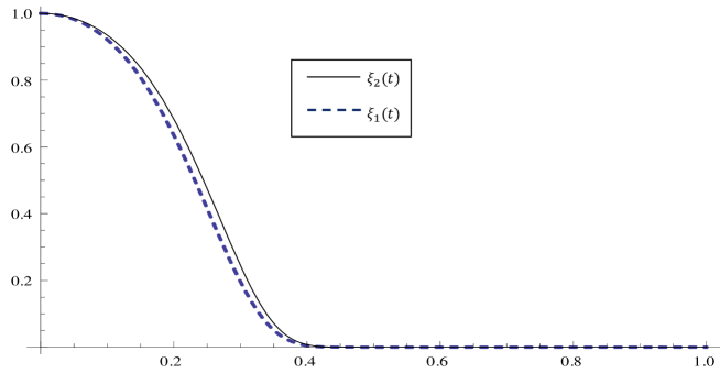
Figure 1: Plot of $\xi_{1}(t)$ and $\xi_{2}(t)$ against $t\in[0,1]$.

In the following example we illustrate the result given in Theorem 3.2.

Example 5.2

Consider two series systems, each comprising of three components having lifetimes following the PO model with the common baseline survival function given by $\bar{F}(x)=e^{-2x}$, $x\geq 0$. Then the survival functions of the two series systems are given by

$$\bar{F}_{X_{1:3}}(x)=\prod_{i=1}^{3}\frac{\lambda_{i}e^{-2x}}{1-\bar{\lambda}_{i}e^{-2x}}\qquad\text{and}\qquad\bar{F}_{Y_{1:3}}(x)=\prod_{i=1}^{3}\frac{\mu_{i}e^{-2x}}{1-\bar{\mu}_{i}e^{-2x}},$$

respectively. Taking $(\lambda_{1},\lambda_{2},\lambda_{3})=(3,4.5,6)$ and $(\mu_{1},\mu_{2},\mu_{3})=(4,5,6)$ we observe that $(3,4.5,6)\stackrel{{\scriptstyle w}}{{\succeq}}(4,5,6)$. Note that

$$\frac{\bar{F}_{Y_{1:3}}(x)}{\bar{F}_{X_{1:3}}(x)}=\left(\frac{120}{81}\right)\left(\frac{1+5.5e^{-2x}+7e^{-4x}}{1+7e^{-2x}+12e^{-4x}}\right),$$

which is increasing in $x\geq 0$, and hence $X_{1:3}\leq_{hr}Y_{1:3}.$ $\hfill\Box$

In the following example we demonstrate the result given in Theorem 3.3

Example 5.3

Consider two series systems, each comprising of four components having lifetimes following the multiple-outlier PO model with the common baseline survival function given by $\bar{F}(x)=e^{-\frac{x^{2}}{2}}$, $x\geq 0$. Then the hazard rate functions of the two series systems are given by

$$r_{X_{1:4}}(x)=\frac{2r(x)}{1-\bar{\lambda_{1}}\bar{F}(x)}+\frac{2r(x)}{1-\bar{\lambda_{2}}\bar{F}(x)},$$ (5.2)

and

$$r_{Y_{1:4}}(x)=\frac{2r(x)}{1-\bar{\mu_{1}}\bar{F}(x)}+\frac{2r(x)}{1-\bar{\mu_{2}}\bar{F}(x)},$$ (5.3)

respectively, where $r(\cdot)$ is the common hazard rate function of each of the components, and $\lambda_{1}=2,\lambda_{2}=4.5,\mu_{1}=3,\mu_{2}=3.5$, so that $(2,2,4.5,4.5)\stackrel{{\scriptstyle m}}{{\succeq}}(3,3,3.5,3.5)$. In order to change the scale, we substitute $x=t/(1-t)$ in (5.2) and (5.3) so that, for $x\in[0,\infty)$, we have $t\in[0,1)$, and after this substitution, let us denote the expressions in (5.2) and (5.3) as $l_{1}(t)$ and $l_{2}(t)$, respectively. From Figure 2(a) we observe that $l_{1}(t)/l_{2}(t)$ is decreasing in $t\in[0,1)$, which is equivalent to the fact that $r_{X_{1:4}}(x)/r_{Y_{1:4}}(x)$ is decreasing in $x\geq 0$. Hence $X_{1:4}\gtrsim_{hr}Y_{1:4}.$ $\hfill\Box$

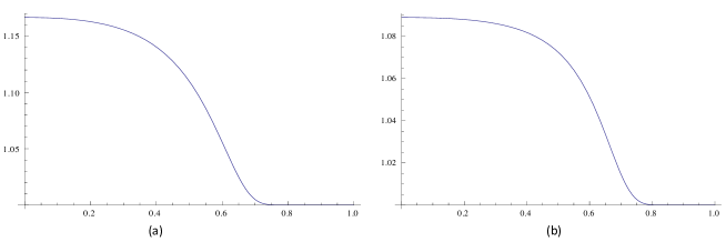
Figure 2: (a) Plot of $l_{1}(t)/l_{2}(t)$ against $t\in[0,1]$, (b) Plot of $\kappa_{1}(t)/\kappa_{2}(t)$ against $t\in[0,1]$.

An application of Theorem 3.5 is given below.

Example 5.4

Consider Example 5.3 with $\lambda_{1}=3,\lambda_{2}=\mu_{2}=\eta=4,\mu_{1}=3.5$, so that $(2,2,4,4)\stackrel{{\scriptstyle w}}{{\succeq}}(3.5,3.5,4,4)$. After substituting $x=t/(1-t)$ in (5.2) and (5.3), let us denote the expressions in (5.2) and (5.3) as $\kappa_{1}(t)$ and $\kappa_{2}(t)$, respectively. From Figure 2(b) we observe that $\kappa_{1}(t)/\kappa_{2}(t)$ is decreasing in $t\in[0,1)$, which implies that $r_{X_{1:4}}(x)/r_{Y_{1:4}}(x)$ is decreasing in $x\geq 0$. Hence $X_{1:4}\gtrsim_{hr}Y_{1:4}.$ $\hfill\Box$

In the following example we demonstrate the result given in Theorem 3.6.

Example 5.5

Consider Example 5.3 with $\lambda_{1}=2,\lambda_{2}=4,\mu_{1}=3,\mu_{2}=3.5$, so that $(2,2,4,4)\stackrel{{\scriptstyle w}}{{\succeq}}(3,3,3.5,3.5)$ and $\lambda_{1}<\mu_{1}<\mu_{2}<\lambda_{2}$. After substituting $x=t/(1-t)$ in (5.2) and (5.3), let us denote the expressions in (5.2) and (5.3) as $\zeta_{1}(t)$ and $\zeta_{2}(t)$, respectively. From Figure 3 we observe that $\zeta_{1}(t)/\zeta_{2}(t)$ is decreasing in $t\in[0,1)$, which is equivalent to the fact that $r_{X_{1:4}}(x)/r_{Y_{1:4}}(x)$ is decreasing in $x\geq 0$. Hence $X_{1:4}\gtrsim_{hr}Y_{1:4}.$ $\hfill\Box$

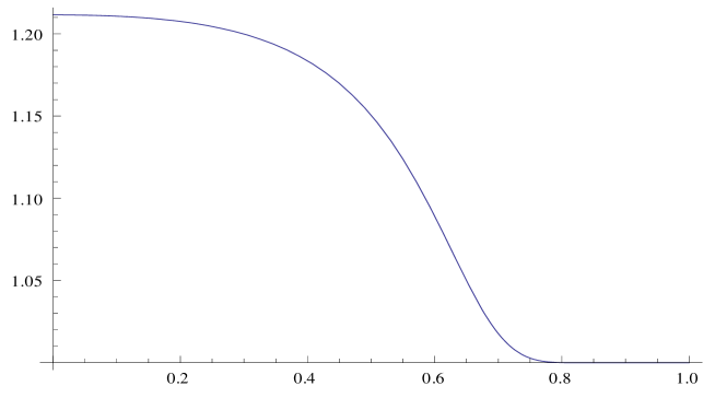
Figure 3: Plot of $\zeta_{1}(t)/\zeta_{2}(t)$ against $t\in[0,1]$.

Below we give an example to illustrate the result given in Theorem 4.1.

Example 5.6

Consider two parallel systems, each comprising of three components having lifetimes following the PO model with the common baseline survival function given by $\bar{F}(x)=e^{-1.5x}$, $x\geq 0$. Then the reversed hazard rate functions of two parallel systems are given by

$$\tilde{r}_{X_{3:3}}(x)=\frac{1.5e^{-1.5x}}{1-e^{-1.5x}}\sum_{i=1}^{3}\frac{\lambda_{i}}{1-\bar{\lambda}_{i}e^{-1.5x}}$$ (5.4)

and

$$\tilde{r}_{Y_{3:3}}(x)=\frac{1.5e^{-1.5x}}{1-e^{-1.5x}}\sum_{i=1}^{3}\frac{\mu_{i}}{1-\bar{\mu}_{i}e^{-1.5x}},$$ (5.5)

respectively, where $(\lambda_{1},\lambda_{2},\lambda_{3})=(0.5,2.5,4)$ and $(\mu_{1},\mu_{2},\mu_{3})=(1,3,5)$ so that $(0.5,2.5,4)\stackrel{{\scriptstyle w}}{{\succeq}}(1,3,5)$. In order to change the scale, we substitute $x=t/(1-t)$ in (5.4) and (5.5) so that, for $x\in[0,\infty)$, we have $t\in[0,1)$, and after this substitution, let us denote the expressions in (5.4) and (5.5) as $\gamma_{1}(t)$ and $\gamma_{2}(t)$, respectively. From Figure 4 we observe that $\gamma_{1}(t)\leq\gamma_{2}(t),\;t\in[0,1)$, which implies that $\tilde{r}_{X_{3:3}}(x)\leq\tilde{r}_{Y_{3:3}}(x)$ for all $x\geq 0$. Hence $X_{3:3}\leq_{rhr}Y_{3:3}$. $\hfill\Box$

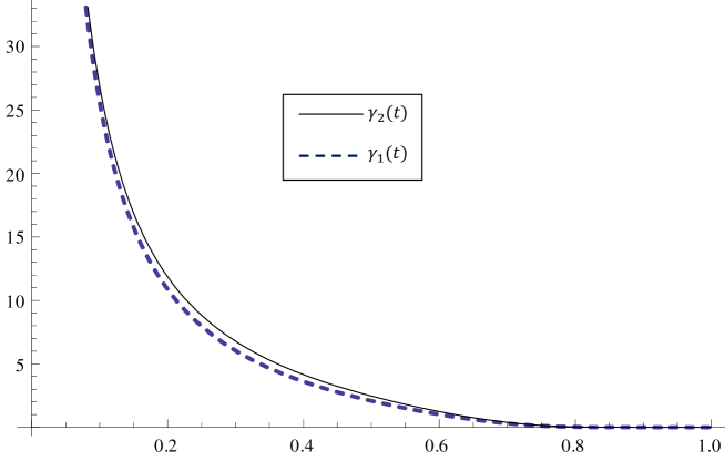
Figure 4: Plot of $\gamma_{1}(t)$ and $\gamma_{2}(t)$ against $t\in[0,1]$.

The following example demonstrates the results given in Theorems 4.3 and 4.4.

Example 5.7

Consider two parallel systems, each comprising of four components having lifetimes following the multiple-outlier PO model with the common baseline survival function given by $\bar{F}(x)=e^{-2x}$, $x\geq 0$. Then the ratio of the reversed hazard rate functions of two parallel systems is given by

$$\frac{\tilde{r}_{Y_{4:4}}(x)}{\tilde{r}_{X_{4:4}}(x)}=\frac{\frac{2\mu_{1}}{1-\bar{\mu_{1}}e^{-2x}}+\frac{2\eta}{1-\bar{\eta}e^{-2x}}}{\frac{2\lambda_{1}}{1-\bar{\lambda_{1}}e^{-2x}}+\frac{2\eta}{1-\bar{\eta}e^{-2x}}},$$ (5.6)

where $\lambda_{1}=2,\eta=3,\mu_{1}=4,$ so that $\lambda_{1}<\eta<\mu_{1}$. Note that $\tilde{r}_{Y_{4:4}}(x)/\tilde{r}_{X_{4:4}}(x)$ is increasing in $x\geq 0$. Hence $X_{4:4}\lesssim_{rhr}Y_{4:4}.$ Again, we have

$$\frac{f_{Y_{4:4}}(x)}{f_{X_{4:4}}(x)}=\left(\frac{F_{Y_{4:4}}(x)}{F_{X_{4:4}}(x)}\right)\left(\frac{\tilde{r}_{Y_{4:4}}(x)}{\tilde{r}_{X_{4:4}}(x)}\right).$$

It can be verified that $F_{Y_{4:4}}(x)/F_{X_{4:4}}(x)=(1+e^{-2x})^{2}/(1+3e^{-2x})^{2}$ is increasing in $x\geq 0$, which implies that $f_{Y_{4:4}}(x)/f_{X_{4:4}}(x)$ is increasing in $x\geq 0$. Hence $X_{4:4}\leq_{lr}Y_{4:4}.$

5.2 Counterexamples

A list of counterexamples are discussed in this subsection. The following counterexample shows that the $p$-larger order in Theorem 3.1 cannot be replaced by reciprocal majorization order.

Counterexample 5.1

Let $X=(X_{1},X_{2},X_{3})$ and $Y=(Y_{1},Y_{2},Y_{3})$ with $X_{i}\sim PO(\bar{F},\lambda_{i})$ and $Y_{i}\sim PO(\bar{F},\mu_{i})$, $i=1,2,3$, where the baseline survival function $\bar{F}$ is given by $\bar{F}(x)=e^{-2x},\;x>0$. Take $(\lambda_{1},\lambda_{2},\lambda_{3})=(2.2,3,5)$ and $(\mu_{1},\mu_{2},\mu_{3})=(2.8,3.2,3.3)$ so that $(\lambda_{1},\lambda_{2},\lambda_{3})\stackrel{{\scriptstyle rm}}{{\succeq}}(\mu_{1},\mu_{2},\mu_{3})$ but $(\lambda_{1},\lambda_{2},\lambda_{3})\stackrel{{\scriptstyle p}}{{\nsucceq}}(\mu_{1},\mu_{2},\mu_{3})$. It is observed that, for $x=0.2$, $\bar{F}_{X_{1:3}}(x)=0.63929$ and $\bar{F}_{Y_{1:3}}(x)=0.641646$. Again, for $x=0.8$, $\bar{F}_{X_{1:3}}(x)=0.0861549$ and $\bar{F}_{Y_{1:3}}(x)=0.084394$. So $X_{1:3}\nleq_{st}Y_{1:3}$. $\Box$

Below we show that weak majorization order in Theorem 3.2 cannot be replaced by $p$-larger order.

Counterexample 5.2

Let $X=(X_{1},X_{2},X_{3})$ and $Y=(Y_{1},Y_{2},Y_{3})$ with $X_{i}\sim PO(\bar{F},\lambda_{i})$ and $Y_{i}\sim PO(\bar{F},\mu_{i})$, $i=1,2,3$, where the baseline survival function $\bar{F}$ is given by $\bar{F}(x)=e^{-1.2x},\;x>0$. Take $(\lambda_{1},\lambda_{2},\lambda_{3})=(2,3,5)$ and $(\mu_{1},\mu_{2},\mu_{3})=(2.8,3.2,3.4)$ so that $(\lambda_{1},\lambda_{2},\lambda_{3})\stackrel{{\scriptstyle p}}{{\succeq}}(\mu_{1},\mu_{2},\mu_{3})$ but $(\lambda_{1},\lambda_{2},\lambda_{3})\stackrel{{\scriptstyle w}}{{\nsucceq}}(\mu_{1},\mu_{2},\mu_{3})$. It is observed that, for $x=0.2$, $r_{X_{1:3}}(x)=1.4273$ and $r_{Y_{1:3}}(x)=1.3516$, and, for $x=1.8$, $r_{X_{1:3}}(x)=2.8722$ and $r_{Y_{1:3}}(x)=2.8907$. Thus, we have $X_{1:3}\nleq_{hr}Y_{1:3}$. $\Box$

In Theorem 3.3, we have seen that, in the case of multiple-outlier model, out of two series systems formed from heterogeneous components, one may dominate the other in relative ageing in terms of hazard rate, provided the two sets of the parameters of the model have majorization order between them. However, this kind of result may not hold for parallel systems as we see in the following counterexample.

Counterexample 5.3

Let $X=(X_{1},X_{2},...,X_{6})$ and $Y=(Y_{1},Y_{2},...,Y_{6})$, each follows the multiple-outlier PO model such that $X_{i}\sim PO(\bar{F},2)$, $Y_{i}\sim PO(\bar{F},3)$, for $i=1,2$, $X_{j}\sim PO(\bar{F},6)$, $Y_{j}\sim PO(\bar{F},5.5)$, for $j=3,4,5,6$, where the baseline survival function is given by $\bar{F}(x)=e^{-2x},\;x>0$. Clearly, $(2,2,6,6,6,6)\stackrel{{\scriptstyle m}}{{\succeq}}(3,3,5.5,5.5,5.5,5.5)$. However, it is observed from Figure 5(a) that $\tilde{r}_{Y_{6:6}}(x)/\tilde{r}_{X_{6:6}}(x)$ is non-monotone. $\Box$

That weak supermajorization order in Theorem 4.1 cannot be replaced by $p$-larger order is shown in the following counterexample.

Counterexample 5.4

Let $X=(X_{1},X_{2},X_{3})$ and $Y=(Y_{1},Y_{2},Y_{3})$ with $X_{i}\sim PO(\bar{F},\lambda_{i})$ and $Y_{i}\sim PO(\bar{F},\mu_{i})$, $i=1,2,3$, where the baseline survival function is given by $\bar{F}(x)=e^{-1.8x}$, $x>0$. Take $(\lambda_{1},\lambda_{2},\lambda_{3})=(2,3,5)$ and $(\mu_{1},\mu_{2},\mu_{3})=(2.6,3.2,3.7)$ so that $(\lambda_{1},\lambda_{2},\lambda_{3})\stackrel{{\scriptstyle p}}{{\succeq}}(\mu_{1},\mu_{2},\mu_{3})$ but $(\lambda_{1},\lambda_{2},\lambda_{3})\stackrel{{\scriptstyle w}}{{\nsucceq}}(\mu_{1},\mu_{2},\mu_{3})$. It is observed that, for $x=1.5$, $\bar{F}_{X_{3:3}}(x)=0.471629$ and $\bar{F}_{Y_{3:3}}(x)=0.459619$ so that $X_{3:3}\nleq_{st}Y_{3:3}$. Now, take $(\lambda_{1},\lambda_{2},\lambda_{3})=(2.5,3,5)$ and $(\mu_{1},\mu_{2},\mu_{3})=(3,3.8,4.4)$ which give $(\lambda_{1},\lambda_{2},\lambda_{3})\stackrel{{\scriptstyle p}}{{\succeq}}(\mu_{1},\mu_{2},\mu_{3})$. It is observed that, for $x=1.2$, $\bar{F}_{X_{3:3}}(x)=0.67176$ and $\bar{F}_{Y_{3:3}}(x)=0.69449$ so that $X_{3:3}\ngeq_{st}Y_{3:3}$. $\Box$

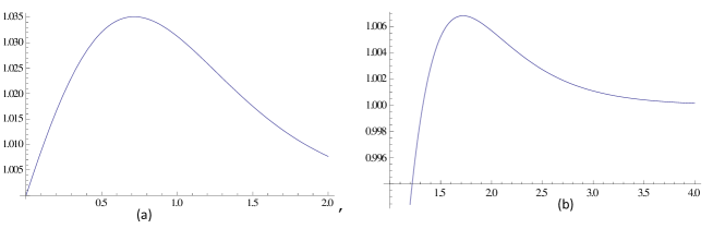
Figure 5: (a) Curve of $\tilde{r}_{Y_{6:6}}(x)/\tilde{r}_{X_{6:6}}(x)$ (b) Curve of $f_{Y_{6:6}}(x)/f_{X_{6:6}}(x)$

Counterexample 5.5

Let $X=(X_{1},X_{2},X_{3},X_{4})$ and $Y=(Y_{1},Y_{2},Y_{3},Y_{4})$, each follows the multiple-outlier PO model such that $X_{i}\sim PO(\bar{F},\lambda_{i})$, $i=1,2,3,4$ and $Y_{i}\sim PO(\bar{F},\lambda)$, $i=1,2,3,4$, where the baseline survival function is given by $\bar{F}(x)=e^{-(x/\beta)^{k}}$, $\beta,k>0,\;x>0$. It is observed from Figure 6(a) that, for $\lambda_{1}=2$, $\lambda_{2}=3$, $\lambda_{3}=4$, $\lambda_{4}=5$, $\lambda=3.6$, $\beta=0.8$, and $k=2$, $\tilde{r}_{Y_{4:4}}(x)/\tilde{r}_{X_{4:4}}(x)$ is non-monotone. Again, for $\lambda_{1}=2$, $\lambda_{2}=3$, $\lambda_{3}=4$, $\lambda_{4}=5$, $\lambda=3.4$, $\beta=3$ and $k=2$, $\tilde{r}_{Y_{4:4}}(x)/\tilde{r}_{X_{4:4}}(x)$ is also non-monotone as can be seen from Figure 6(b). $\Box$

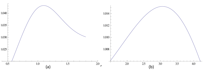
Figure 6: (a) Curve of $\tilde{r}_{Y_{4:4}}(x)/\tilde{r}_{X_{4:4}}(x)$ for $(\lambda_{1},\lambda_{2},\lambda_{3},\lambda_{4},\lambda,\beta,k)=(2,3,4,5,3.6,0.8,2)$, and (b) Curve of $\tilde{r}_{Y_{4:4}}(x)/\tilde{r}_{X_{4:4}}(x)$ for $(\lambda_{1},\lambda_{2},\lambda_{3},\lambda_{4},\lambda,\beta,k)=(2,3,4,5,3.4,3,2)$

That the condition $\lambda_{1}\leqslant\eta\leqslant\mu_{1}$ in Theorem 4.3 cannot be dropped is shown below.

Counterexample 5.6

Let $X_{1}$ and $X_{2}$ follow the PO model with parameters $\lambda_{1}$ and $\eta$ respectively, and let $Y_{1}$ and $Y_{2}$ follow the PO model with parameters $\mu_{1}$ and $\eta$ respectively, where the baseline distribution is exponential with parameter $\lambda=2$. Now, for $\lambda_{1}=0.2$, $\mu_{1}=0.4$ and $\eta=0.9$, $\tilde{r}_{Y_{2:2}}(x)/\tilde{r}_{X_{2:2}}(x)$ is non-monotone, as we see from Figure 7.

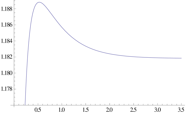
Figure 7: Curve of $\tilde{r}_{Y_{2:2}}(x)/\tilde{r}_{X_{2:2}}(x)$

6 Conclusion

In this paper, we have studied stochastic comparison of series and parallel systems formed from independent heterogeneous components having lifetimes following the PO model. Most of the results are obtained using different concepts of majorization. We have also compared a system formed of heterogeneous components with another system of homogeneous components. We have derived conditions under which two series systems with heterogeneous components are ordered with respect to different stochastic orders; in the case of multiple-outlier model, they are compared with respect to likelihood ratio order and relative ageing in terms of hazard rate. We have also derived conditions under which a series system with heterogeneous components and that with homogeneous components are ordered with respect to the above mentioned stochastic orderings. In the case of parallel system, we have obtained conditions under which two parallel systems with heterogeneous components are ordered with respect to the usual stochastic order and reversed hazard rate order. The comparison is also made in the case of a parallel system with heterogeneous components and that with homogeneous components. However, unlike series system, with suitable counterexamples, we have shown that, even in the case of multiple-outlier model, under majorization order, two parallel systems with heterogeneous components may not be comparable with respect to likelihood ratio order and relative ageing in terms of reversed hazard rate, although, under more restricted conditions, we are able to compare the parallel systems with respect to those stochastic orderings.

Similar kinds of results can be studied for a $k$-out-of-$n$ system or equivalently, for $r$th largest order statistic (see the explanation given in the introduction in this regard). It can be noted that the expressions for different reliability functions $viz.$, survival function, hazard rate function, reversed hazard rate function etc. corresponding to an order statistic coming from different heterogeneous populations are not very explicit in nature and hence similar treatment as above cannot be used to handle these problems. We are planning to study different ordering results for the $k$-out-of-$n$ system of heterogeneous populations under multiple-outlier models, and then extend these results to the general model.

References

- Balakrishnan and Zhao (2013) Balakrishnan, N., Zhao, P. (2013). Hazard rate comparison of parallel systems with heterogeneous gamma components, Journal of Multivariate Analysis 113, 153-160.
- Bennet (1983) Bennett, S. (1983). Analysis of survival data by the proportional odds model, Statistics in Medicine 2, 273-277.
- Bon and Pǎltǎnea (1999) Bon, J.L., Pǎltǎnea, E. (1999). Ordering properties of convolutions of exponential random variables, Lifetime Data Analysis 5, 185-192.
- Bon and Pǎltǎnea (2006) Bon, J.L., Pǎltǎnea, E. (2006). Comparisons of order statistics in a random sequence to the same statistics with i.i.d. variables, ESAIM: Probability and Statistics 10, 1-10.
- Collett (2004) Collett, D. (2015). Modelling survival data in medical research, 2nd edition, Chapman and Hall/CRC, Boca Raton.
- Cordeiro et al. (2014) Cordeiro, G.M., Lemonte, A.J., Ortega, E.M.M. (2014). The Marshall-Olkin family of distributions: mathematical properties and new models, Journal of Statistical Theory and Practice 8(2), 343-366.
- Dinse and Lagakos (1983) Dinse, G.E., Lagakos, S.W. (1983). Regression analysis of tumour prevalence data, Applied Statistics 32(3), 236-248.
- Dykstra et al. (1997) Dykstra, R., Kochar, S.C., Rojo, J. (1997). Stochastic comparisons of parallel systems of heterogeneous exponential components, Journal of Statistical Planning and Inference 65, 203-211.
- Fang and Balakrishnan (2016) Fang, L., Balakrishnan N. (2016). Ordering results for the smallest and largest order statistics from independent heterogeneous exponential-Weibull random variables, Statistics 50, 1195-1205.
- Fang and Zhang (2012) Fang, L., Zhang, X. (2012). New results on stochastic comparison of order statistics from heterogeneous Weibull populations, Journal of Korean Statistical Society 41, 13-16.
- Fang and Zhang (2015) Fang, L., Zhang, X. (2015). Stochastic comparison of parallel system with exponentiated Weibull components, Statistics & Probability Letters 97, 25-31.
- Gupta et al. (2015) Gupta, N., Patra, L.K., Kumar, S. (2015). Stochastic comparisons in systems with Frèchet distributed components, Operations Research Letters 43, 612-615.
- Hazra et al. (2017) Hazra, N.K., Kuiti, M.R., Finkelstein, M., Nanda, A.K. (2017). On stochastic comparisons of maximum order statistics from the Location-Scale family of distributions, Journal of Multivariate Analysis 160, 31-41.
- Hazra et al. (2018) Hazra, N.K., Kuiti, M.R., Finkelstein, M., Nanda, A.K. (2018). On stochastic comparisons of minimum order statistics from the Location-Scale family of distributions, Metrika 81, 105-123.
- Kayal (2019) Kayal, S. (2019). Stochastic comparisons of series and parallel systems with Kumaraswamy-G distributed components, American Journal of Mathematical and Management Sciences, 38(1), 1-22.
- Khaledi and Kochar (2000) Khaledi, B., Kochar, S.C. (2000). Some new results on stochastic comparisons of parallel systems, Journal of Applied Probability 37, 283-291.