Analysis of nonlocal phonon thermal conductivity simulations showing the ballistic to diffusive crossover

Abstract

Simulations (e.g. Zhou et al., Phys. Rev. B 79, 115201 (2009)) show nonlocal effects of the ballistic/diffusive crossover. The local temperature has nonlinear spatial variation not contained in the local Fourier law $\vec{j}(\vec{r})=-\kappa\vec{\nabla}T(\vec{r})$. The heat current $\vec{j}(\vec{r})$ depends not just on the local temperature gradient $\vec{\nabla}T(\vec{r})$, but also on temperatures at points $\vec{r}^{\ \prime}$ within phonon mean free paths, which can be micrometers long. This paper uses the Peierls-Boltzmann transport theory in non-local form to analyze the spatial variation $\Delta T(\vec{r})$. The relaxation-time approximation (RTA) is used because full solution is very challenging. Improved methods of extrapolation to obtain the bulk thermal conductivity $\kappa$ are proposed. Callaway invented an approximate method of correcting RTA for the $\vec{q}$ (phonon wavevector or crystal momentum) conservation of N (normal as opposed to Umklapp) anharmonic collisions This method is generalized to the non-local case where $\kappa(\vec{k})$ depends on wavevector of the current $\vec{j}(\vec{k})$ and temperature gradient $i\vec{k}\Delta T(\vec{k})$.

I Introduction

Figure 1 shows a molecular dynamics (MD) simulation for insulating wurtzite-structure GaN. It shows the spatial change of temperature $\Delta T(x)$ driven by steady heat input $P(x)$ in regions near $x=nL\pm L/2$ and equal steady heat removal near $x=nL$. This MD study by Zhou et al. Zhou et al. (2009) illustrates nicely the nonlocal relation between temperature gradient $\nabla_{x}T$ and heat current $j(x)$.

Figure 1: Heat flow simulation by Zhou et al. Zhou et al. (2009) for wurtzite-structure GaN. A segment of length $L=500c=2600\AA$ (along the $c$-axis) and cross section $A=15\sqrt{3}a^{2}=264\AA^{2}$, containing 60,000 atoms, was periodically repeated in all directions. The average temperature was $\bar{T}=$301.2K. Heat $Pd=0.003$eV/ps$\AA^{2}$ (volumetric heating rate $7.7\times 10^{18}$W/m³) was added at segments of width $d=12c$ at $-L/2$ (and equivalently at $+L/2$) and extracted at $L=0$. These regions are shown by the solid black lines. In the regions of length $L/2-d$ between heat insertion and removal, a constant heat current $j=0.0015$ eV/ps$\AA^{2}=2.4\times 10^{10}$W/m² flows. The temperature was averaged in 100 discrete segments of width $5c$. The gradient $dT/dx=\pm 0.0265$K$/\AA$ computed at midpoints $\pm L/4$ corresponds to $\kappa(L)=-j/(dT/dx)=$90.4W/mK. This number will increase by a significant amount (perhaps a factor more than 2) for a very long simulation cell. An “effective” thermal conductivity can be defined by using the mean temperatures $T_{H}$ and $T_{C}$ of the regions of heating and cooling. Then $(T_{H}-T_{C})/(L/2)$ is a mean temperature gradient, giving $\kappa_{\rm eff}=55$W/mK.

Because of the care and accuracy of the simulation, and also because the system studied was periodic (with period $L$ which enables Fourier space analysis with discrete wavevectors $2\pi m/L$), it is nicely suited for deeper analysis. The current paper argues that the spatial variation of $\Delta T(x)$ is the property most interesting for study, not the “effective conductivity” or similar constructs that may be more easily measurable. In a separate paper Allen and Perebeinos (2018) the concept of “thermal susceptibility” ($\Theta$ where $\Delta T(\vec{r})=\int d\vec{r}^{\ \prime}\Theta(\vec{r}-\vec{r}^{\ \prime})P(\vec{r}^{\ \prime})$) is introduced. It has an inverse relation to thermal conductivity, much as the charge susceptibility has an inverse relation to electrical conductivity.

In small insulators, with size $L$ similar to the long mean free paths $\ell$ of small $|\vec{q}|$ (long wavelength) acoustic phonons, heat transport deviates from the local Fourier law $\vec{j}(\vec{r})=-\kappa\vec{\nabla}T(\vec{r})$. This is topic has attracted attention for more than 25 years Cahill et al. (2014); Majumdar (1993); Joshi and Majumdar (1993); Chen (1998, 2001). The terminology “ballistic/diffusive crossover” is common. Diffusive heat propagation gives the local Fourier law, but ballistic heat propagation requires (in linear approximation) a nonlocal kernel $\vec{j}(\vec{r})=-\int d\vec{r}^{\ \prime}\kappa(\vec{r},\vec{r}^{\ \prime})\vec{\nabla}T(\vec{r}^{\ \prime})$. The range of the kernel is $|\vec{r}-\vec{r}^{\ \prime}|\sim\ell$. Interesting (and technologically important) non-local effects happen if $\vec{r}$ is within a distance $\ell$ of a heat source or sample boundary.

Advances in measurement Gomès et al. (2015) include coherent x-ray thermal probing of strip-line arrays Siemens et al. (2010); Hoogeboom-Pot et al. (2015); Zeng et al. (2015), transient thermal gratings Maznev et al. (2011); Johnson et al. (2013); Hua and Minnich (2014a); Huberman et al. (2017), and time-domain thermal reflectance Minnich et al. (2011); Ding et al. (2014); Wilson and Cahill (2014). Theory has become increasingly powerful Hua and Minnich (2014b); Vermeersch (2016); Vermeersch and Mingo (2018) and evolves togther with experiment Minnich (2012); Collins et al. (2013); Minnich (2015).

My tool for analysis of the “data” of Fig. 1 is the Peierls-Boltzmann equation (PBEPeierls (1929); Ziman (1960)). The PBE must treat explicitly the sources and sinks of heat, since they are at distances $\sim L/4$ from the source, and this is not larger than $\ell_{Q}$ for many important phonon modes $Q$. My analysis benefits from recent improvements, which include an explicit heat source term in the PBE Hua and Minnich (2014b); Vermeersch et al. (2015), and a Fourier-transformed ($\vec{k}$-space) version of the PBE Hua and Minnich (2014b); Allen (2014). The PBE is not as microscopic as an MD simulation, which can approximate exact atom-level motions (treated classically). Boltzmann theory, on the other hand, uses phonon quasiparticles. The particle (rather than wave) picture is used, and requires wave-packets. The spatial resolution of Boltzmann theory is thus limited by the size of the wave-packet, i.e. not shorter than a phonon wavelength. Crystalline matter is spatially inhomogeneous at the atomic level, but spatially homogeneous at length scales greater than lattice constants. Thus Boltzmann analysis of crystals gives a non-local thermal conductivity $\kappa(\vec{r},\vec{r}^{\ \prime})$ invariant under the simultaneous translation $\vec{r}\rightarrow\vec{r}+\vec{s},\ \ \vec{r}^{\ \prime}\rightarrow\vec{r}^{\ \prime}+\vec{s}$. In atomic level theory, the translations $\vec{s}$ are the lattice translation vectors. However, the PBE is insensitive to this distance scale, so $\vec{s}$ can be regarded as arbitrary and continuous. Thus $\kappa$ can be written as $\kappa(\vec{r}-\vec{r}^{\ \prime})$, and can be represented in $\vec{k}$-space as $\kappa(\vec{k})$, rather than as $\kappa(\vec{k}+\vec{G},\vec{k}+\vec{G}^{\prime})$. On the other hand, the PBE treats phonons as quantum objects, and is thus not limited to the high $T$ classical limit where MD simulation works.

In this paper, $Q$ will always refer to the quantum numbers $(\vec{q},s)$ of a phonon, and $\vec{k}$ (or $k=|\vec{k}|$) will denote the reciprocal space coordinate (or wavevector) of a field (like heat current, $\vec{j}$). The same symbol is used for functions (like $j(x)$ or $\kappa(x-x^{\prime})$) in coordinate space and in reciprocal space (e.g. $j(k)$ and $\kappa(k)$). The three-dimensional Fourier relations are defined as $j(\vec{r})=(1/N)\sum_{\vec{k}}j(\vec{k})\exp(i\vec{k}\cdot\vec{r})$ and $j(\vec{k})=(1/\Omega_{\rm cell})\int d\vec{r}j(\vec{r})\exp(-i\vec{k}\cdot\vec{r})$, with $N$ the number of unit cells in the crystal and $\Omega_{\rm cell}$ the volume of the crystal primitive cell. This paper concerns nanoscales in one direction, chosen as $x$ (as in Fig. 1). The other directions are macroscopic. Therefore reciprocal space behavior involves $k_{y}=k_{z}=0$, and $k_{x}$ is abbreviated as $k$.

Fig. 1 is a steady state nonequilibrium molecular dynamics (NEMD) simulation for GaN, with steady heat insertion and removal at a controlled rate, in widely separated and narrow spatial regions. Therefore the heat current $j(x)=j$ is steady, and known, in the regions between heat insertion and removal. Therefore the curvature of $T(x)$ evident in Fig. 1 is a clear sign of a nonlocal connection between $j$ and $T$. The system had average $T\approx 300$K; classical trajectories were computed from an empirical interatomic force law. Local temperatures $T(x_{i})=<KE>_{i}/3Nk_{B}$ were computed by time averaging the kinetic energy $KE$ of all $N_{i}$ atoms in slabs (labeled $i$) containing $N_{i}=600$ atoms. The aim of the simulation was to make the total length $L$ large enough to achieve the diffusive limit, so that $\kappa$ could be found by computing $\Delta T/\Delta x$ in central slabs. However, GaN at 300K has many phonons with mean free paths exceeding the sample size $L$, so the fully diffusive limit was not reached. Extrapolation was attempted by the model $\kappa(L)\approx\kappa(\infty)-\kappa^{\prime}/L$. The current paper provides better extrapolation models. The extrapolated value was well below the experimental 230 W/mK Slack et al. (2002); Jezowski et al. (2003). Interestingly, theory Lindsay et al. (2012) now shows that isotopically pure GaN (as assumed in the simulation) should have $\kappa$(300K)$\approx$400 W/mK. It is not clear whether finite size or an inadequate model potential $V(R)$ is the main culprit limiting the realism of the simulation. However, for the purpose of this paper, material-specific realism is irrelevant. The model is useful for studying nonlocality, because of the care and accuracy of the simulation, independent of possible problems with the potential.

The curvature of $T(x)$ seen in the figure was regarded as a nuisance or an artifact of the finite size. The alternative view advocated here is that Fig. 1 simulates an idealized experiment, not yet achievable. This “experiment” reveals details of nonlocality, and probes nicely the ballistic to diffusive crossover.

This simulation is simple to analyze for two reasons. (1) Periodicity $f(x+L)=f(x)$ is maintained for all fields. (2) Regions of heat input and extraction are “transparent” to propagating phonon modes. A thermostat occasionally perturbs atom trajectories in discrete regions, but does not alter the lattice periodicity that gives homogeneously propagating phonon modes. The response function $\kappa(x-x^{\prime})$ has periodicity $L$ in $x-x^{\prime}$, and wavevectors in $\kappa(k)$ are quasi-discrete ($k=2\pi n/L$) and Bloch-periodic ($k\equiv k+2\pi/a$). If instead a simulation had a hard wall or other disruption of homogeneity, the Boltzmann equation would not separate when written in $k$-space, and numerical solution to find $T(x)$ would be challenging. Most actual nanoscale heat transport involves spatial inhomogeneity. However, exceptions such as “transient thermal grating” (TTG) experiments Rogers et al. (1994), and the idealized experiments analyzed by Hua and Minnich Hua and Minnich (2018), can be analyzed by the method used here.

Accurate solutions of the full PBE for bulk thermal conductivity have been available for several years Broido et al. (2007); Chernatynskiy and Phillpot (2010); Li et al. (2014). Several recent papers Koh et al. (2014); Ordonez-Miranda et al. (2015); Hua and Minnich (2014b, 2015); Maassen and Lundstrom (2015); Kaiser et al. (2017); Cepellotti and Marzari (2017a, b) find solutions of the PBE containing nonlocal effects.

The outline of this paper is: Section II discusses the discrete Fourier transform used to convert Fig. 1 to Fig. 2. Section III discusses the nonlocal PBE, and solves it using the relaxation-time approximation (RTA). Section IV gives numerical answers using a Debye model. Section V gives the nonlocal generalization of Callaway’s approximation for Normal (N) and Umklapp (U) collisions. Section VI shows how best to extrapolate simulation data to the bulk limit. In Appendix A, boundary-condition influences on nanoscale non-locality are discussed. Appendix B gives detailed analytic formulas for various versions of the Debye model, and Appendix C gives details of the Callaway version of the theory.

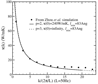
Figure 2: The dots are nonlocal $\kappa(k)$ constructed for GaN at 300K, by Fourier transforming the $T(x)$ results shown in Fig. 1. The curves are Debye-model RTA theoretical fits, discussed in Sec. IV. The same two adjustable parameters ($\kappa_{0}=$80 W/mK and $\ell_{\rm min}=83\AA$) are used in both curves. If the phonon scattering rate $1/\tau_{Q}\propto\omega^{2}$ (i.e. $p=2$) is used, the bulk limit $\kappa(k\rightarrow 0)$ is $3\kappa_{0}=240\AA$. If exponent $p=3$ is chosen, $\kappa(k)$ diverges as $|\log(k)|$ as $k\rightarrow 0$.

II Fourier transforms

The information in Fig. 1 is Fourier transformed following Ref. Allen, 2014. The resulting values of $\kappa(k)$ are shown in Fig. 2. Because the simulation of Fig. 1 has $M$=100 discrete segments, the wavevector $k$ must have only $M=100$ possible values $k_{n}=2\pi n/L$ for $-M/2+1\leq n\leq M/2$, where $L/M=w=5c$ is the width of the separate segments where $T$ is averaged. But there are only $M/4$ independent real numbers in the computed $\Delta T(x)$, since $\Delta T(-x)$ converges to the same value as $\Delta T(x)$, and $\Delta T(L/4+x)$ converges to the same value as $-\Delta T(L/4-x)$ (barring small non-linear effects). Therefore there are only $M/4=25$ real numbers in the Fourier representation, which can be taken as the values of $\kappa(k_{n})$ for positive odd integers $n$. Only the smallest 12 $k_{n}$’s are shown in Fig. 2. Higher $k_{n}$’s are increasingly noisy. Partly this is caused by noise in the original calculations, and partly by additional noise in the digitization (original numerical information was not available.)

III Boltzmann $\kappa(k)$

GaN is a good thermal conductor; its phonons have long mean free paths. Thus it is a good “phonon gas” and should be accurately treated by the Boltzmann equation. The fundamental object of Boltzmann theory is the distribution function $N_{Q}$, which gives the average occupation at $(\vec{r},t)$ in coordinate space, or $(\vec{k},\omega)$ in reciprocal space, of phonon mode $Q$. Its evolution is given by the equation,

$$\frac{\partial N_{Q}}{\partial t}=\left(\frac{dN_{Q}}{dt}\right)_{\rm drift}+\left(\frac{dN_{Q}}{dt}\right)_{\rm scatt}+\left(\frac{dN_{Q}}{dt}\right)_{\rm ext}.$$ (1)

The result shown in Fig. 1 has reached steady state in a time-independent thermal driving, so $\partial N_{Q}/\partial t=0$. The driving is one-dimensional, so the resulting current density is

$$j(x)=\frac{1}{\Omega_{S}}\sum_{Q}\hbar\omega_{Q}v_{Qx}N_{Q}(x)$$ (2)

where $\vec{v}_{Q}$ is the group velocity of mode $Q$ and $\Omega_{S}=N\Omega_{\rm cell}$ is the sample volume. An identical equation applies to the reciprocal space relation between $j(k)$ and $N_{Q}(k)$.

The scattering term in a non-metal includes defect scattering which couples $N_{Q}$ to $N_{Q^{\prime}}$, and anharmonic scattering which couples $N_{Q}$ to ($N_{Q+Q^{\prime}}$, $N_{-Q^{\prime}}$). A local equilibrium Bose-Einstein distribution $n_{Q}=[\exp(\hbar\omega_{Q}/k_{B}T(x))-1]^{-1}$ is the only distribution that is stationary ($[dN_{Q}/dt]_{\rm scatt}=0$) under collisions. For weak driving, the scattering term can be linearized to the form

$$\left(\frac{dN_{Q}}{dt}\right)_{\rm scatt} = -\sum_{Q^{\prime}}S_{Q,Q^{\prime}}\Phi_{Q^{\prime}}$$

$$\Phi_{Q^{\prime}}(x) = N_{Q^{\prime}}(x)-n_{Q^{\prime}}(T(x)),$$ (3)

where the linearized scattering operator $S_{Q,Q^{\prime}}$ is non-negative Ziman (1960). It can be made real-symmetric by multiplying by $n_{Q^{\prime}}(n_{Q^{\prime}}+1)$. Its eigenvalues are all greater than 0 except for one zero eigenvalue related to conservation of phonon energy. The rate of change of energy density caused by collisions is

$$0=\left(\frac{dU}{dt}\right)_{\rm scatt}=-\frac{1}{\Omega_{S}}\sum_{QQ^{\prime}}\hbar\omega_{Q}S_{QQ^{\prime}}\Phi_{Q^{\prime}}.$$ (4)

Since this must hold for any possible deviation $\Phi_{Q}$ from equilibrium, then $\hbar\omega_{Q}$ must be a null left eigenvector of the scattering matrix,

$$\sum_{Q}\hbar\omega_{Q}S_{QQ^{\prime}}=0.$$ (5)

This relation (which will be invoked later) and other aspects are discussed elsewhere Allen and Perebeinos (2018). The diagonal elements $S_{Q,Q}$ are the “single-mode relaxation rates” $1/\tau_{Q}$.

The “drift” term in Eq.(1) has the form

$$\left(\frac{dN_{Q}}{dt}\right)_{\rm drift}=-\vec{v}_{Q}\cdot\vec{\nabla}N_{Q}=-\vec{v}_{Q}\cdot\left[\frac{dn_{Q}}{dT}\vec{\nabla}T+\vec{\nabla}\Phi_{Q}\right]$$ (6)

The rate of energy change caused by drift is

$$\left(\frac{dU}{dt}\right)_{\rm drift} = \frac{1}{\Omega_{S}}\sum_{Q}\hbar\omega_{Q}\left(\frac{dN_{Q}}{dt}\right)_{\rm drift}$$ (7)

$$= -\frac{1}{\Omega_{S}}\sum_{Q}\hbar\omega_{Q}\vec{v}_{Q}\cdot\vec{\nabla}\Phi_{Q}=-\vec{\nabla}\cdot\vec{j}.$$

The external driving term deserves discussion:

$$\left(\frac{dN_{Q}}{dt}\right)_{\rm ext}=\frac{P(x)}{C}\frac{dn_{Q}}{dT}.$$ (8)

The need for such a term was only recently recognized Hua and Minnich (2014b, 2015); Vermeersch et al. (2015), and was incorrectly omitted in an earlier paper Allen (2014). The specific form on the right-hand side of Eq. 8 is not unique, but depends on the geometry being modeled. This version, used in ref. Vermeersch et al., 2015, is appropriate for the Zhou et al. simulation Zhou et al. (2009): the thermostat is designed to increase occupancies $N_{Q}$ of modes at the same rate that a uniform rate of temperature increase $\dot{T}=P/C$ would cause an equilibrated system to increase $n_{Q}(T(t))$. $P(x)$ is the volume rate of heating at spatial point $x$, and $C$ is the volumetric heat capacity. Then the total volumetric energy input is

$$\left(\frac{dU}{dt}\right)_{\rm ext}=\frac{1}{\Omega_{S}}\sum_{Q}\hbar\omega_{Q}\left(\frac{dN_{Q}}{dt}\right)_{\rm ext}=P(x),$$ (9)

Energy conservation as given by Eqs. 1, 4, 7, and 9 is

$$\frac{\partial U}{\partial t}=0=P-\vec{\nabla}\cdot\vec{j}.$$ (10)

Since we consider steady state situations with time-independent driving, $\partial U/\partial t=0$.

The full linearized PBE now takes the form

$$\vec{v}_{Q}\cdot\left[\frac{dn_{Q}}{dT}\vec{\nabla}T+\vec{\nabla}\Phi_{Q}\right]+\sum_{Q^{\prime}}S_{Q,Q^{\prime}}\Phi_{Q^{\prime}}=\frac{P}{C}\frac{dn_{Q}}{dT}.$$ (11)

Here the fields $T=T_{0}+\Delta T(\vec{r})$, $\Phi_{Q}$, and $P$ are all in coordinate ($\vec{r}$) space. The equation simplifies in reciprocal space. For the one-dimensional version, this is

$$ikv_{Qx}\left[\frac{dn_{Q}}{dT}\Delta T(k)+\Phi_{Q}(k)\right] + \sum_{Q^{\prime}}S_{Q,Q^{\prime}}\Phi_{Q^{\prime}}(k)$$ (12)

$$= \frac{P(k)}{C}\frac{dn_{Q}}{dT},$$

where $\nabla_{x}T(x)\rightarrow ik\Delta T(k)$. Solution requires inversion of a non-Hermitean $Q$-space matrix $\hat{S}+ikv_{x}\hat{1}$. For many purposes it is sufficient to make the “single-mode relaxation time approximation” (RTA), $S_{Q,Q^{\prime}}\rightarrow\delta_{Q,Q^{\prime}}/\tau_{Q}$. This permits a simple solution,

$$\Phi_{Q}(k)=-\frac{dn_{Q}}{dT}\frac{[ikv_{Qx}\Delta T(k)-P(k)/C]}{1/\tau_{Q}+ikv_{Qx}}.$$ (13)

We now want to eliminate the field $P(k)$. This can be done Allen and Perebeinos (2018) using local energy conservation, as advocated in Refs. Hua and Minnich, 2014b, 2015; Vermeersch et al., 2015. The form used in these papers is

$$\sum_{Q}\hbar\omega_{Q}(N_{Q}-n_{Q})/\tau_{Q}=0,$$ (14)

which is the RTA version of Eq. 4. This equation is not satisfied in RTA for arbitrary $\Phi_{Q}$, but it is sensible to require the chosen steady state distribution to satisfy it. Equivalently, one can use $P(k)=i\vec{k}\cdot\vec{j}(k)$.

From Eqs. 2 and 3, the current can be written as

$$j_{x}(k)=\frac{1}{\Omega_{S}}\sum_{Q}\hbar\omega_{Q}v_{Qx}\Phi_{Q}(k)$$ (15)

since the equilibrium distribution $n_{Q}$ carries no current. Then the current satisfies

$$Z(k)j_{x}(k)=-\kappa_{1}(k)\nabla_{x}T(k)$$ (16)

where $\kappa_{1}$ comes from the first term on the right of Eq. 13,

$$\kappa_{1}(k)=\frac{1}{\Omega_{S}}\sum_{Q}\frac{\hbar\omega_{Q}v_{Qx}^{2}(dn_{Q}/dT)}{1/\tau_{Q}+ikv_{Qx}}.$$ (17)

The function $\kappa_{1}$ is the nonlocal thermal conductivity that comes from incorrectly omitting the external driving, Eq. 8. It is the phonon analog of the Reuter-Sondheimer theory Reuter and Sondheimer (1948) of the anomalous skin effect contained in the electrical conductivity $\sigma(\vec{k},\omega)$ in the dc ($\omega=0$) limit.

The subscript $1$ in Eq. 17 indicates omission of a “renormalization” factor $1/Z(k)$ (or equivalently, setting $Z$ to 1). $Z(k)$ contains the effects of the driving term, and has the form

$$Z(k)=1-\sum_{Q}\frac{C_{Q}}{C}\frac{ikv_{Qx}}{1/\tau_{Q}+ikv_{Qx}},$$ (18)

and $C_{Q}$ is $\hbar\omega_{Q}(dn_{Q}/dT)/\Omega_{S}$, the contribution to the heat capacity $C$ from mode Q. Since $\sum_{Q}C_{Q}/C=1$, the renormalization factor can be written as

$$Z(k)=\sum_{Q}\frac{C_{Q}}{C}\frac{1/\tau_{Q}}{1/\tau_{Q}+ikv_{Qx}}=\sum_{Q}\frac{C_{Q}}{C}\frac{1}{1+k^{2}\ell_{Qx}^{2}}.$$ (19)

where $\ell_{Qx}=v_{Qx}\tau_{Q}$. Then the thermal conductivity in PBE theory with RTA is

$$\kappa(k)=\kappa_{1}(k)/Z(k).$$ (20)

This equation is different in appearance but is equivalent to those in Refs. Hua and Minnich, 2014b; Vermeersch et al., 2015.

IV Debye $\kappa(k)$

In the bulk limit, if $T$ is not too low, the RTA is known to reproduce quite well the true solution, if $1/\tau_{Q}$ is the actual complicated single mode phonon relaxation rate. For qualitative understanding, simpler models are desirable. In the Debye model there are three acoustic phonon branches, all having the form $\omega_{Q}=v|\vec{q}|$, all with the same velocity $v$. As a supplement to the Debye model, take the relaxation rates $1/\tau_{Q}$ to have simple power laws in phonon wavevector $|\vec{q}|$, $(1/\tau_{D})(q/q_{D})^{p}$. Here $q_{D}$ is the Debye wavevector, and $1/\tau_{D}$ is a maximum scattering rate, which depends on $T$, being linear in $T$ at higher $T$. The scale of $\kappa(T)$ in the Debye model is

$$\kappa_{0}=\frac{k_{B}v^{2}\tau_{D}}{\Omega_{\rm cell}},$$ (21)

which depends on $T$ because of $\tau_{D}$.

In Debye approximation, Eqs.(17,19) become, in the classical ($k_{B}T>\hbar\omega_{D}$) limit,

$$\kappa_{1D}(k)=\frac{9k_{B}v^{2}}{2\Omega_{\rm cell}}\int_{0}^{Q_{D}}\frac{dQQ^{2}}{Q_{D}^{3}}\int_{-1}^{1}\frac{\mu^{2}d\mu}{1/\tau_{Q}+ikv\mu}$$ (22)

$$Z_{D}(k)=\frac{3}{2}\int_{0}^{Q_{D}}\frac{dQQ^{2}}{Q_{D}^{3}}\int_{-1}^{1}d\mu\frac{1/\tau_{Q}}{1/\tau_{Q}+ikv\mu}$$ (23)

where $\mu$ is $\cos\theta$, and $\theta$ is the angle between the velocity (parallel to $\vec{q}$) and the direction of the temperature gradient (parallel to $\vec{k}=k\hat{x}$). A factor of 3 appears in Eq.(22), to account for the three acoustic branches.

There is no complete consensus about what the power $p$ should be. Herring Herring (1954) advocated $p=2$, and has received experimental confirmation Damen et al. (1999). However, subsequent studies Esfarjani et al. (2011); Ma et al. (2014); Zhou et al. (2016) differ somewhat. Often, for “N” (Normal, $\sum\vec{q}$ conserved) scattering, $p=2$, while for “U” (Umklapp, $\sum\vec{q}$ altered by a reciprocal lattice vector $\vec{G}$), $p=3$. For general $p$, Eqs.(22,23) become

$$\kappa_{1Dp}(k)=\frac{9\kappa_{0}}{2}\int_{0}^{1}dx\int_{-1}^{1}d\mu\frac{x^{2}\mu^{2}}{x^{p}+iy\mu}$$ (24)

$$Z_{Dp}(k)=\frac{3}{2}\int_{0}^{1}dx\int_{-1}^{1}d\mu\frac{x^{2}x^{p}}{x^{p}+iy\mu}$$ (25)

where $x=q/q_{D}$ and $y=kv\tau_{D}=k\ell_{\rm min}$. Algebraic formulas for these integrals are given in Appendix B. When $T\gg\Theta_{D}$ is not obeyed, Eqs.(24,25) each need a quantum factor $(x\gamma_{T}/\sinh(x\gamma_{T}))$ inside the $x$-integral, where $\gamma_{T}=\hbar\omega_{D}/2k_{B}T$.

The answers simplify at large wavevector $k\ell_{\rm min}>>1$,

$$\kappa_{1Dp}(k) \rightarrow \frac{9\kappa_{0}}{(3+p)(k\ell_{\rm min})^{2}}$$

$$Z_{Dp} \rightarrow \frac{3\pi}{(3+p)2k\ell_{\rm min}}$$

$$\kappa_{Dp}\equiv\kappa_{1DP}/Z_{Dp} \rightarrow \frac{6\kappa_{0}}{\pi k\ell_{\rm min}}$$ (26)

However, Boltzmann theory for the statistical evolution of $N_{Q}(\vec{r})$ is hard to justify on atomic distance scales, or at wavevectors $k$ as large as a reciprocal lattice vector $G=2\pi/a$. The secure small $k\ell_{\rm min}=y$ part of the formulas for $\kappa_{1Dp}$ (Eq. 24) is

$$(p=0)\ \ \kappa_{1D0}(k)\sim\kappa_{0}(1-3y^{2}/5+\ldots)$$

$$(p=1)\ \ \kappa_{1D1}(k)\sim\frac{3}{2}\kappa_{0}\left(1-\frac{6}{5}y^{2}\log\frac{1}{y}+\ldots\right)$$

$$(p=2)\ \ \kappa_{1D2}(k)\sim 3\kappa_{0}\left(1-\frac{3\pi}{7}\sqrt{\frac{y}{2}}+\ldots\right)$$

$$(p=3)\ \ \kappa_{1D3}(k)\sim\kappa_{0}\left(\log\frac{1}{y}+\ldots\right)$$ (27)

Notice that the small $k$ parts for $p\geq 1$ have non-analytic $k$-dependences, and the $p=3$ formula diverges logarithmically. Similarly, the small $k$ results for $Z_{Dp}$ (Eq. 25) are

$$(p=0)\ \ Z_{D0}(k)\sim 1-y^{2}/3+\ldots)$$

$$(p=1)\ \ Z_{D1}(k)\sim 1-y^{2}+\ldots$$

$$(p=2)\ \ Z_{D2}(k)\sim 1-\frac{3\pi\sqrt{2}}{10}y^{3/2}+\ldots$$

$$(p=3)\ \ Z_{D3}(k)\sim 1-\pi y/4+\ldots$$ (28)

Full results from Eqs.(24,25) are in Fig. 3. The full theories $\kappa_{Dp}=\kappa_{1Dp}/Z_{Dp}$ agree with the unrenormalized results $\kappa_{1Dp}$ at small $k$. Notice that at large $k$, in agreement with Eq. 26, the full theories converge to an answer independent of exponent $p$. This relates to the fact that large $k$ corresponds to small distances where results should not depend on mean free paths, which are all longer than the distance scale. However, the unrenormalized curves fall off faster with $k$ and shift depending on $p$.

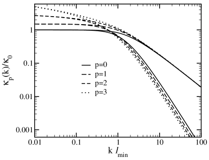
Figure 3: Power law Debye models for $\kappa(k)/\kappa_{0}$ at high $T$. These are derived from the models $1/\tau_{Q}\propto Q^{p}\propto\omega^{p}$ and $p=0,1,2,3$. The four cases each have one curve at small $k\ell_{\rm min}$, which splits into two curves at large $k\ell_{\rm min}$. The upper branches are numerical solutions of the full high $T$ Boltzmann theory in the RTA/Debye model, Eq. 20. The lower branches are $\kappa_{1}(k)$, Eq. 17, for the same models, omitting the renormalization $Z$. The $p=2$ and $3$ full versions are shown on a linear scale in Fig. 2.

V Callaway $\kappa(k)$

Callaway Callaway (1959); Allen (2013) devised an improved version of the relaxation time approximation. Because of anharmonic terms in the interatomic potential, a phonon $Q$ with wavevector $\vec{q}$ can decay into two phonons of wavevector $\vec{q}_{1}+\vec{q}_{2}$ provided $\vec{q}=\vec{q}_{1}+\vec{q}_{2}+\vec{G}$. The N processes have the reciprocal lattice vector $\vec{G}=0$, and the U processes have $\vec{G}\neq 0$. Peierls Peierls (1929) pointed out that N processes cannot fully relax the heat current. This is particularly important at lower $T$, because U processes require higher energy phonons and are thus suppressed at lower $T$.

Callaway’s model for the rate of change of the phonon distribution $N_{Q}$ is

$$\left(\frac{dN_{Q}}{dt}\right)_{\rm collision}=-\frac{N_{Q}-n_{Q}}{\tau_{QU}}-\frac{N_{Q}-n_{Q}^{\ast}}{\tau_{QN}}$$ (29)

The distribution $n_{Q}^{\ast}$ is the one which maximizes entropy subject to conservation of both energy and wavevector. It is a modified Bose-Einstein distribution

$$n_{Q}^{\ast}=\frac{1}{\exp(\hbar\omega_{Q}/k_{B}T+\Lambda_{x}q_{x})-1},$$ (30)

where $\Lambda_{x}$ is a Lagrange multiplier fixed by the condition $\sum_{Q}q_{x}n_{Q}^{\ast}=q_{x,\rm tot}=\sum_{Q}q_{x}\Phi_{Q}$. The natural extension of Debye-type relaxation laws in the Callaway scheme is

$$1/\tau_{Q} = 1/\tau_{QU}+1/\tau_{QN}=(1/\tau_{D})(r_{U}x^{3}+r_{N}x^{2})$$

$$1/\tau_{QU} = 1/\tau_{U}(q/q_{D})^{3}=(1/\tau_{D})r_{U}x^{3}$$

$$1/\tau_{QN} = 1/\tau_{N}(q/q_{D})^{2}=(1/\tau_{D})r_{N}x^{2}$$ (31)

where $r_{U}$ and $r_{N}$ are the relative rates of U and N scattering, with $r_{U}+r_{N}=1$. The coefficients $r_{U}$ and $r_{N}$ depend strongly on $T$ at low $T$, but are $T$-independent at higher $T$ (where $1/\tau_{D}\propto T$).

Zhou et al. Zhou et al. (2016) computed relaxation rates for GaAs in the classical limit. The results in Fig. 2 of their paper indicate that $r_{U}\sim 0.9$ and $r_{N}\sim 0.1$. One could expect similar values for GaN. The Boltzmann equation (12) can be written in Callaway form and solved. The Callaway result (with both $r_{N}$ and $r_{U}$ non-zero) cures the logarithmic divergence ($\kappa\propto\log L$) obtained when purely $p=3$ Umklapp scattering is used, and gives a finite $\kappa(k\rightarrow 0)$ limit. Appendix C contains the derivation of the Callaway correction to the nonlocal theory for $\kappa(k)$. Unfortunately, the data shown in Fig. 2 do not extend to low enough $k$ to enable a choice to be made about actual relaxation rates and how they are distributed between N and U processes.

VI extrapolating $\kappa$ to $L\rightarrow\infty$

Zhou et al. Zhou et al. (2009) attempt extrapolation of their finite size ($L$) simulations to $L\rightarrow\infty$, and notice difficulties. The present results require alternate extrapolations. One way is to choose a model relaxation time and use the resulting Debye RTA theory to fit the $\kappa(k)$ curves in Fig. 2. Three things should be stressed. First, the theoretical curves do not give a particularly good fit to the higher $k$ part of $\kappa(k)$. This is not surprising. Debye approximation describes small $Q$ phonon properties, but does not recognize the small group velocities and corresponding small mean free paths of optical modes. These modes do carry heat, and are not suppressed at larger $k$. Second, a surprisingly nice fit with no theory at all can be made by plotting $\log\kappa(k)$ versus $\log k$. This is shown in Fig. 4. The result, that $\kappa(k)$ is roughly proportional to $k^{-0.75}$, should not be taken seriously, even though it is as good a fit as any obtained from Debye RTA theory. A $k^{-0.75}$ divergence implies a scaling $\kappa_{\rm bulk}\propto L^{0.75}$ which has never been detected experimentally, and is almost certainly unphysical. Nevertheless, it is an intriguing observation which might motivate further investigation of behavior of $\kappa(k)$ in vibrational heat conductors. The third thing to be stressed is that fitting the $\kappa(k)$ data is an imperfect enterprise. The numerical $T(x)$ data of Zhou et al. shown in Fig. 1 were not originally intended for this purpose. The $k$-points for which numbers can be found are too sparse for confident fits, and are affected by noise of computation and digitization.

Figure 4: The $\kappa(k)$ data from Fig. 2 are plotted here on a logarithmic scale, showing an approximate $\kappa\propto 1/k^{0.75}$ fit. This diverges strongly as $k\rightarrow 0$. The accuracy of this fit is probably accidental, because there is no theory to justify it.

Nevertheless, theory makes relevant points. The fits shown in Fig. 2 provide understanding of the unexpectedly fast increase of $\kappa(k)$ as $k$ decreases. They also provide two kinds of guidance for extrapolation. First there is direct use of theory and numerics for $\kappa(k)$. The two curves in Fig. 2, when extended to $k=0$, yield

$$(p=2)\ \ \kappa(0)=3\kappa_{0}\sim 240{\rm\ W/mK}$$

$$(p=3)\ \ \kappa(0)=\infty\times\kappa_{0}\sim\infty$$

(32)

Evidently extrapolation to $L\rightarrow\infty$ is even more uncertain than imagined by Zhou et al..

The other version of extrapolation indicated by this analysis is, following Zhou et al., to plot $\kappa(L)$ obtained from the temperature slope at mid-point, against various functions of $L$. Zhou et al. used $\kappa(\infty)-\kappa^{\prime}/L$. Formulas derived here show that $\kappa(\infty)-\kappa^{\prime}/\sqrt{L}$ has more theoretical justification and better correspondence with the computed $\kappa(k)$.

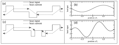
Figure 5: Choice (a) is standard and used in Fig. 1. The others are suggested alternative heating profiles The sine curve (b) is the simplest. The asymmetrical block heating (c) allows all Fourier components to be extracted. Two sines (curve (d)) allows $k=2\pi/L$ and $4\pi/L$ to be extracted simultaneously.

Finally, Fig. 5 suggests alternate ways of performing NEMD simulations. A more rapid reduction of noise will happen if instead of insertion of heat into separate isolated regions (panel a), the heat is inserted sinusoidally (panel b). This has been tested Li and Allen (2014) with some success for a simple model. But this gives only a single $k$-point for $\kappa(k)$, while a mesh of small-$k$ points contains much additional insight. The heating pattern could use more than one sinusoidal period, as in Fig. 5d. Finally, it is frustrating that the analysis done here yields only $k_{n}$ with odd integer $n$; if $n=2,4,6$ were available to supplement $n=1,3,5$, then theoretical fits could be judged with more confidence. The even integers were excluded by the mirror symmetry of the heat input. For example, the mirror in panel (a) is around $x=0$, and in panel (b), around $x=L/4$. Arrangements like those shown in panels (c) and (d) provide the desired symmetry breaking.

VII acknowledgements

I am grateful to Chengyun Hua, Mengkun Liu, A. J. H. McGaughey, A. J. Minnich, V. Perebeinos, P. K. Schelling, and Xiaowang Zhou for useful advice. I thank M. V. Fernandez-Serra and J. Siebert for inspiration. This work was supported in part by DOE grant No. DE-FG02-08ER46550.

VIII appendix A: Boundary effects in Simulations

The characteristic sigmoid shape seen in the Zhou et al. Zhou et al. (2009) simulations of Fig. 1 is not always as prominent in other simulations. Comparison of various simulations indicates that the detailed expression of non-locality differs depending on boundary conditions. For slab problems, either “transparent” or “opaque” boundary conditions are used. With transparent boundaries, the unperturbed simulation cell is repeated periodically in all three directions. Heat is added and removed somewhere in the cell interior. With opaque boundaries, periodicity of the simulation cell in the direction of heat flow is irrelevant. Homogeneity is broken, and atoms near the boundary have to respond, not to a periodic image, but to the actual heated boundary. Analysis of such situations Hua and Minnich (2015) (which can be experiment or simulation) requires a model of how the boundary emits and reflects vibrations. The temperature distributions near the boundary can therefore vary. This paper deals only with the simpler transparent version. Other examples (besides Zhou et al.) of simulations with transparent boundaries are Aubry et al. Aubry et al. (2008), Goel et al. Goel et al. (2015), and Gordiz and Henry Gordiz and Henry (2017). Examples of opaque boundaries are Landry and McGaughey Landry and McGaughey (2009), Jiang et al. Jiang et al. (2009), Cao and Qu Cao and Qu (2012), and Feng et al. Feng et al. (2017).

IX Appendix B: Analytic Integrations

For integer $p$, the integrations in Eqs.(24,25) can be done analytically:

$$\frac{\kappa_{1D0}(k)}{\kappa_{0}}=\frac{3}{y^{2}}\left[1-\frac{\tan^{-1}(y)}{y}\right]$$ (33)

$$\frac{\kappa_{1D1}(k)}{\kappa_{0}}=\frac{9}{10}\left[1+\frac{2}{y^{2}}\left(1-\frac{\tan^{-1}(y)}{y}\right)-y^{2}\log\left(1+\frac{1}{y^{2}}\right)\right]$$ (34)

$$\frac{\kappa_{1D2}(k)}{\kappa_{0}} = \frac{9}{7y^{2}}\left\{1-\frac{\tan^{-1}(y)}{y}+2y^{2}\right.$$ (35)

$$- \frac{y^{5/2}}{\sqrt{2}}\left[\tan^{-1}\left(\sqrt{\frac{2}{y}}+1\right)+\tan^{-1}\left(\sqrt{\frac{2}{y}}-1\right)\right]$$

$$- \left.\frac{y^{5/2}}{2\sqrt{2}}\log\left(\frac{1+\sqrt{2y}+y}{1-\sqrt{2y}+y}\right)\right\}$$

$$\frac{\kappa_{1D3}(k)}{\kappa_{0}}=\frac{1}{2}\log\left(\frac{1+y^{2}}{y^{2}}\right)+\frac{1}{y^{2}}\left(1-\frac{\tan^{-1}(y)}{y}\right)$$ (36)

$$Z_{D0}=\frac{\tan^{-1}y}{y}$$ (37)

$$Z_{D1}=\frac{1}{4}-\frac{3y^{2}}{4}+\frac{3\pi y^{3}}{8}+\frac{3}{4}(1-y^{4})\frac{\tan^{-1}y}{y}$$ (38)

$$Z_{D2} = \frac{1}{20y}\left\{8y+12\tan^{-1}y-6\sqrt{2}y^{5/2}\left[\tan^{-1}\left(1+\sqrt{\frac{2}{y}}\right)\right.\right.$$

$$+ \left.\left.\tan^{-1}\left(1-\sqrt{\frac{2}{y}}\right)\right]+3\sqrt{2}y^{5/2}\log\left(\frac{1+\sqrt{2y}+y}{1-\sqrt{2y}+y}\right)\right\}$$

$$Z_{D3}=\frac{1}{2}-\frac{\pi y}{4}+(1+y^{2})\frac{\tan^{-1}y}{2y}$$ (40)

These equations are plotted versus $y=k\ell_{\rm min}$ in Fig. 3.

X Appendix C: Nonlocal Callaway Model

In the full PBE, both “Normal” (N) and “Umklapp” (U) scattering events are contained in the linearized scattering operator $S_{Q,Q^{\prime}}$. The total crystal momentum $\sum_{Q}\vec{q}N_{Q}$ is automatically conserved under N-scattering alone. That is, if only N terms of $S_{Q,Q^{\prime}}$ are kept, $\sum_{Q}\vec{q}N_{Q}$ is conserved. At low $T$, where U-scattering is suppressed relative to N, it is important to recognize the different effects of these two types of events. Callaway therefore introduced a modified version of the relaxation time approximation,

$$\left(\frac{dN_{Q}}{dt}\right)_{\rm scatt}\rightarrow-\frac{N_{Q}-n_{Q}}{\tau_{QU}}-\frac{N_{Q}-n_{Q}^{\ast}}{\tau_{QN}}$$ (41)

where

$$n_{Q}^{\ast}=\frac{1}{\exp(\hbar\omega_{Q}/k_{B}T+\vec{q}\cdot\vec{\Lambda})-1}\approx n_{Q}-\frac{dn_{Q}}{dT}\frac{k_{B}T^{2}}{\hbar\omega_{Q}}\vec{q}\cdot\vec{\Lambda},$$ (42)

and $\vec{\Lambda}$ is a Lagrange multiplier, adjusted so that the distribution $n_{Q}^{\ast}$ contains all the crystal momentum. That means

$$\sum_{Q}\vec{q}N_{Q}=\sum_{Q}\vec{q}n_{Q}^{\ast}$$ (43)

or, since the equilibrium distribution $n_{Q}$ has no net crystal momentum,

$$\sum_{Q}\vec{q}\Phi_{Q}=-\sum_{Q}\frac{dn_{Q}}{dT}\frac{k_{B}T^{2}}{\hbar\omega_{Q}}\vec{q}\vec{q}\cdot\vec{\Lambda}$$ (44)

The total single-mode scattering rate $1/\tau_{Q}=S_{QQ}$ is

$$1/\tau_{Q}=1/\tau_{QU}+1/\tau_{QN}.$$ (45)

Because of the last term of Eq. 42, the Boltzmann equation has an additional term, and the RTA solution, Eq. 13 takes the form

$$\Phi_{Q}(k)=-\frac{dn_{Q}}{dT}\frac{[\vec{v}_{Q}\cdot\vec{\nabla}T(k)+\frac{k_{B}T^{2}}{\hbar\omega_{Q}\tau_{QN}}\vec{q}\cdot\vec{\Lambda}-\frac{P(k)}{C}]}{1/\tau_{Q}+i\vec{k}\cdot\vec{v}_{Q}}.$$ (46)

Now it is necessary to have two additional equations, because the two extra fields $P(k)$ and $\vec{\Lambda}(k)$ need to be eliminated. These equations are energy conservation (Eqs. 14 and 15) for eliminating $P$ and crystal momentum conservation (Eq. 44) for $\vec{\Lambda}$. The result of using Eq. 14 to eliminate $P/C$ is a minor extension of the previous result, Eq. 20, containing the same renormalization factor $Z$, in Eq. 19. To avoid $3\times 3$ matrix equations, orthorhombic or higher symmetry is now assumed, and one-dimensional transport along an orthorhombic axis denoted $x$. This permits $\vec{q}\cdot\vec{\Lambda}$ to be simplified to $q_{x}\Lambda$. The current density is

$$j_{x}=-\frac{\kappa_{1}}{Z}\frac{dT}{dx}-\frac{k_{B}T^{2}}{\Omega_{S}Z}\sum_{Q}\frac{dn_{Q}}{dT}\frac{v_{Qx}/\tau_{QN}}{1/\tau_{Q}+ikv_{Qx}}q_{x}\Lambda.$$ (47)

Here $\kappa_{1}$ is the same as before, Eq. 17, with both N and U processes included in the scattering $1/\tau_{Q}$ as in Eq. 45. The second term in Eq. 47 is an additional current that comes from the fact that the scattering caused by N processes has been overestimated in the first term. The new formula for the distribution function is

$$\Phi_{Q}=-\frac{1}{Z}\frac{dn_{Q}}{dT}\frac{v_{Qx}\nabla T+\frac{k_{B}T^{2}}{\hbar\omega_{Q}\tau_{QN}}q_{x}\Lambda}{1/\tau_{Q}+ikv_{Qx}}.$$ (48)

Now use Eq. 44 to eliminate the Lagrange multiplier $\Lambda$. After some algebra, the result for the Callaway heat conductivity $\kappa_{C}(k)$ can be written

$$\kappa_{C}(k)=\frac{\kappa_{1}}{Z}+\frac{1}{Z\Omega_{S}}\frac{\sum_{Q}H_{Qx}\frac{q_{x}}{\tau_{QN}}\sum_{Q^{\prime}}H_{Q^{\prime}x}q_{x}^{\prime}}{\sum_{Q}\frac{dn_{Q}}{dT}\frac{q_{x}^{2}}{\hbar\omega_{Q}}\left[Z-\frac{1/\tau_{QN}}{1/\tau_{Q}+ikv_{Qx}}\right]},$$ (49)

where

$$H_{Qx}=\frac{dn_{Q}}{dT}\frac{v_{Qx}}{1/\tau_{Q}+ikv_{Qx}}.$$ (50)

The second term of Eq. 49 is the Callaway correction to the nonlocal RTA thermal conductivity (when the thermal variation is one-dimensional, and the symmetry orthorhombic or higher.) In the local limit $k\rightarrow 0$ and $Z\rightarrow 1$, this answer agrees exactly with Eq. 15 of Ref. Allen, 2013.

References

- Zhou et al. (2009) X. W. Zhou, S. Aubry, R. E. Jones, A. Greenstein, and P. K. Schelling, “Towards more accurate molecular dynamics calculation of thermal conductivity: Case study of GaN bulk crystals,” Phys. Rev. B 79, 115201 (2009).
- Allen and Perebeinos (2018) P. B. Allen and V. Perebeinos, “Temperature in a Peierls-Boltzmann treatment of nonlocal phonon heat transport,” ArXiv e-prints (2018), arXiv:1803.10757 [cond-mat] .
- Cahill et al. (2014) D. G. Cahill, P. V. Braun, G. Chen, D. R. Clarke, Shanhui Fan, K. E. Goodson, P. Keblinski, W. P. King, G. D. Mahan, A. Majumdar, H. J. Maris, S. R. Phillpot, E. Pop, and Li Shi, “Nanoscale thermal transport. ii. 2003–2012,” Appl. Phys. Revs. 1, 011305 (2014).
- Majumdar (1993) A. Majumdar, “Microscale heat conduction in dielectric thin films,” ASME. J. Heat Transfer 115, 7–16 (1993).
- Joshi and Majumdar (1993) A. A. Joshi and A. Majumdar, “Transient ballistic and diffusive phonon heat transport in thin films,” J. Appl. Phys. 74, 31–39 (1993).
- Chen (1998) G. Chen, “Thermal conductivity and ballistic-phonon transport in the cross-plane direction of superlattices,” Phys. Rev. B 57, 14958–14973 (1998).
- Chen (2001) G. Chen, “Ballistic-diffusive heat-conduction equations,” Phys. Rev. Lett. 86, 2297–2300 (2001).
- Gomès et al. (2015) S. Gomès, A. Assy, and P.-O. Chapuis, “Scanning thermal microscopy: A review,” Phys. Stat. Sol. (a) 212, 477–494 (2015).
- Siemens et al. (2010) M. E. Siemens, Qing Li, Ronggui Yang, K. A. Nelson, E. H. Anderson, M. M. Murnane, and H. C. Kapteyn, “Quasi-ballistic thermal transport from nanoscale interfaces observed using ultrafast coherent soft x-ray beams,” Nature Mat. 9, 26–30 (2010).
- Hoogeboom-Pot et al. (2015) K. M. Hoogeboom-Pot, J. N. Hernandez-Charpak, Xiaokun Gu, T. D. Frazer, E. H. Anderson, Weilun Chao, R. W. Falcone, Ronggui Yang, M. M. Murnane, H. C. Kapteyn, and D. Nardi, “A new regime of nanoscale thermal transport: Collective diffusion increases dissipation efficiency,” Proc. Nat. Acad. Sci. 112, 4846–4851 (2015).
- Zeng et al. (2015) Liping Zeng, K. C. Collins, Yongjie Hu, M. N. Luckyanova, A. A. Maznev, S. Huberman, V. Chiloyan, Jiawei Zhou, K. A. Nelson, and G. Chen, “Measuring phonon mean free path distributions by probing quasiballistic phonon transport in grating nanostructures,” Scientific Reports 5, 17131 (2015).
- Maznev et al. (2011) A. A. Maznev, J. A. Johnson, and K. A. Nelson, “Onset of nondiffusive phonon transport in transient thermal grating decay,” Phys. Rev. B 84, 195206 (2011).
- Johnson et al. (2013) J. A. Johnson, A. A. Maznev, J. Cuffe, J. K. Eliason, A. J. Minnich, T. Kehoe, C. M. Sotomayor Torres, G. Chen, and K. A. Nelson, “Direct measurement of room-temperature nondiffusive thermal transport over micron distances in a silicon membrane,” Phys. Rev. Lett. 110, 025901 (2013).
- Hua and Minnich (2014a) Chengyun Hua and A. J. Minnich, “Transport regimes in quasiballistic heat conduction,” Phys. Rev. B 89, 094302 (2014a).
- Huberman et al. (2017) S. Huberman, V. Chiloyan, R. A. Duncan, Lingping Zeng, Roger Jia, A. A. Maznev, E. A. Fitzgerald, K. A. Nelson, and G. Chen, “Unifying first-principles theoretical predictions and experimental measurements of size effects in thermal transport in SiGe alloys,” Phys. Rev. Materials 1, 054601 (2017).
- Minnich et al. (2011) A. J. Minnich, J. A. Johnson, A. J. Schmidt, K. Esfarjani, M. S. Dresselhaus, K. A. Nelson, and G. Chen, “Thermal conductivity spectroscopy technique to measure phonon mean free paths,” Phys. Rev. Lett. 107, 095901 (2011).
- Ding et al. (2014) D. Ding, X. Chen, and A. J. Minnich, “Radial quasiballistic transport in time-domain thermoreflectance studied using monte carlo simulations,” Appl. Phys. Lett. 104, 143104 (2014).
- Wilson and Cahill (2014) R. B. Wilson and D. G. Cahill, “Anisotropic failure of fourier theory in time-domain thermoreflectance experiments,” Nature Commun. 5, 5075 (2014).
- Hua and Minnich (2014b) Chengyun Hua and A. J. Minnich, “Analytical Green’s function of the multidimensional frequency-dependent phonon Boltzmann equation,” Phys. Rev. B 90, 214306 (2014b).
- Vermeersch (2016) B. Vermeersch, “Compact stochastic models for multidimensional quasiballistic thermal transport,” J. Appl. Phys. 120, 175102 (2016).
- Vermeersch and Mingo (2018) Bjorn Vermeersch and Natalio Mingo, “Quasiballistic heat removal from small sources studied from first principles,” Phys. Rev. B 97, 045205 (2018).
- Minnich (2012) A. J. Minnich, “Determining phonon mean free paths from observations of quasiballistic thermal transport,” Phys. Rev. Lett. 109, 205901 (2012).
- Collins et al. (2013) K. C. Collins, A. A. Maznev, Zhiting Tian, K. Esfarjani, K. A. Nelson, and G. Chen, “Non-diffusive relaxation of a transient thermal grating analyzed with the boltzmann transport equation,” J. Appl. Phys. 114, 104302 (2013).
- Minnich (2015) A. J. Minnich, “Multidimensional quasiballistic thermal transport in transient grating spectroscopy,” Phys. Rev. B 92, 085203 (2015).
- Peierls (1929) R. E. Peierls, “Zur kinetischen Theorie der Wärmeleitung in Kristallen,” Ann. Phys. 395, 1055–1101 (1929).
- Ziman (1960) J. Ziman, Electrons and Phonons (Oxford, London, 1960).
- Vermeersch et al. (2015) B. Vermeersch, J. Carrete, N. Mingo, and A. Shakouri, “Superdiffusive heat conduction in semiconductor alloys. i. theoretical foundations,” Phys. Rev. B 91, 085202 (2015).
- Allen (2014) P. B. Allen, “Size effects in thermal conduction by phonons,” Phys. Rev. B 90, 054301 (2014), This paper incorrectly omits a term in the PBE for the source of heating.
- Slack et al. (2002) G. A. Slack, L. J. Schowalter, D. Morelli, and J. A. Freitas, “Some effects of oxygen impurities on AlN and GaN,” J. Crystal Growth 246, 287 – 298 (2002), proceedings of the International Workshop on Bulk Nitride Semiconductors.
- Jezowski et al. (2003) A. Jezowski, B.A. Danilchenko, M. Bockowski, I. Grzegory, S. Krukowski, T. Suski, and T. Paszkiewicz, “Thermal conductivity of GaN crystals in 4.2 - 300 K range,” Sol. State Commun. 128, 69 – 73 (2003).
- Lindsay et al. (2012) L. Lindsay, D. A. Broido, and T. L. Reinecke, “Thermal Conductivity and Large Isotope Effect in GaN from First Principles,” Phys. Rev. Lett. 109, 095901 (2012).
- Rogers et al. (1994) J. A. Rogers, Y. Yang, and K. A. Nelson, “Elastic modulus and in-plane thermal diffusivity measurements in thin polyimide films using symmetry-selective real-time impulsive stimulated thermal scattering,” Appl. Phys. A 58, 523–534 (1994).
- Hua and Minnich (2018) Chengyun Hua and Austin J. Minnich, “Heat dissipation in the quasiballistic regime studied using the Boltzmann equation in the spatial frequency domain,” Phys. Rev. B 97, 014307 (2018).
- Broido et al. (2007) D. A. Broido, M. Malorny, G. Birner, N. Mingo, and D. A. Stewart, “Intrinsic lattice thermal conductivity of semiconductors from first principles,” Appl. Phys. Lett. 91, 231922 (2007).
- Chernatynskiy and Phillpot (2010) A. Chernatynskiy and S. R. Phillpot, “Evaluation of computational techniques for solving the Boltzmann transport equation for lattice thermal conductivity calculations,” Phys. Rev. B 82, 134301 (2010).
- Li et al. (2014) Wu Li, J. Carrete, N. A. Katcho, and N. Mingo, “ShengBTE: A solver of the Boltzmann transport equation for phonons,” Comp. Phys. Commun. 185, 1747 – 1758 (2014).
- Koh et al. (2014) Yee Kan Koh, D. G. Cahill, and Bo Sun, “Nonlocal theory for heat transport at high frequencies,” Phys. Rev. B 90, 205412 (2014).
- Ordonez-Miranda et al. (2015) J. Ordonez-Miranda, R. Yang, S. Volz, and J. J. Alvarado-Gil, “Steady state and modulated heat conduction in layered systems predicted by the analytical solution of the phonon Boltzmann transport equation,” J. Appl. Phys. 118, 075103 (2015).
- Hua and Minnich (2015) Chengyun Hua and A. J. Minnich, “Semi-analytical solution to the frequency-dependent Boltzmann transport equation for cross-plane heat conduction in thin films,” J. Appl. Phys. 117, 175306 (2015).
- Maassen and Lundstrom (2015) J. Maassen and M. Lundstrom, “A simple Boltzmann transport equation for ballistic to diffusive transient heat transport,” J. Appl. Phys. 117, 135102 (2015).
- Kaiser et al. (2017) J. Kaiser, T. Feng, J. Maassen, X. Wang, X. Ruan, and M. Lundstrom, “Thermal transport at the nanoscale: A Fourier’s law vs. phonon Boltzmann equation study,” J. Appl. Phys. 121, 044302 (2017).
- Cepellotti and Marzari (2017a) A. Cepellotti and N. Marzari, “Boltzmann transport in nanostructures as a friction effect,” Nano Letters 17, 4675–4682 (2017a).
- Cepellotti and Marzari (2017b) A. Cepellotti and N. Marzari, “Transport waves as crystal excitations,” Phys. Rev. Materials 1, 045406 (2017b).
- Reuter and Sondheimer (1948) G. E. H. Reuter and E. H. Sondheimer, “The theory of the anomalous skin effect in metals,” Proc. Roy. Soc. London A: Math., Phys. and Eng. Sciences 195, 336–364 (1948).
- Herring (1954) C. Herring, “Role of low-energy phonons in thermal conduction,” Phys. Rev. 95, 954–965 (1954).
- Damen et al. (1999) E. P. N. Damen, A. F. M. Arts, and H. W. de Wijn, “Experimental verification of Herring’s theory of anharmonic phonon relaxation: ,” Phys. Rev. B 59, 349–352 (1999).
- Esfarjani et al. (2011) K. Esfarjani, G. Chen, and H. T. Stokes, “Heat transport in silicon from first-principles calculations,” Phys. Rev. B 84, 085204 (2011).
- Ma et al. (2014) Jinlong Ma, Wu Li, and Xiaobing Luo, “Examining the Callaway model for lattice thermal conductivity,” Phys. Rev. B 90, 035203 (2014).
- Zhou et al. (2016) J. Zhou, B. Liao, and G. Chen, “First-principles calculations of thermal, electrical, and thermoelectric transport properties of semiconductors,” Semicond. Science and Tech. 31, 043001 (2016).
- Note (1) In metals, a corresponding Boltzmann equation gives a good theory for susceptibility at small and , but does not contain Friedel oscillations at or high frequency plasma oscillations or interband effects. For phonons, there is no analog of either Friedel or plasma oscillations, so breakdown at large is probably gradual.
- Callaway (1959) J. Callaway, “Model for lattice thermal conductivity at low temperatures,” Phys. Rev. 113, 1046–1051 (1959).
- Allen (2013) P. B. Allen, “Improved Callaway model for lattice thermal conductivity,” Phys. Rev. B 88, 144302 (2013).
- Note (2) Callaway used a slightly different and less correct condition; see Ref. \rev@citealpnumAllen2013.
- Li and Allen (2014) Yerong Li and P. B. Allen, arXiv1412.3099 (2014).
- Aubry et al. (2008) S. Aubry, C. J. Kimmer, A. Skye, and P. K. Schelling, “Comparison of theoretical and simulation-based predictions of grain-boundary Kapitza conductance in silicon,” Phys. Rev. B 78, 064112 (2008).
- Goel et al. (2015) N. Goel, E. B. Webb III, A. Oztekin, J. M. Rickman, and S. Neti, “Kapitza resistance at segregated boundaries in -SiC,” J. Appl. Phys. 118, 115101 (2015).
- Gordiz and Henry (2017) K. Gordiz and A. Henry, “Phonon transport at interfaces between different phases of silicon and germanium,” J. Appl. Phys. 121, 025102 (2017).
- Landry and McGaughey (2009) E. S. Landry and A. J. H. McGaughey, “Thermal boundary resistance predictions from molecular dynamics simulations and theoretical calculations,” Phys. Rev. B 80, 165304 (2009).
- Jiang et al. (2009) Jin-Wu Jiang, Jie Chen, Jian-Sheng Wang, and Baowen Li, “Edge states induce boundary temperature jump in molecular dynamics simulation of heat conduction,” Phys. Rev. B 80, 052301 (2009).
- Cao and Qu (2012) Ajing Cao and Jianmin Qu, “Kapitza conductance of symmetric tilt grain boundaries in graphene,” J. Appl. Phys. 111, 053529 (2012).
- Feng et al. (2017) Tianli Feng, Wenjun Yao, Zuyuan Wang, Jingjing Shi, Chuang Li, Bingyang Cao, and Xiulin Ruan, “Spectral analysis of nonequilibrium molecular dynamics: Spectral phonon temperature and local nonequilibrium in thin films and across interfaces,” Phys. Rev. B 95, 195202 (2017).