On nonlinear fractional maps:
Nonlinear maps with power-law memory

Abstract

This article is a short review of the recent results on properties of nonlinear fractional maps which are maps with power- or asymptotically power-law memory. These maps demonstrate the new type of attractors - cascade of bifurcations type trajectories, power-law convergence/divergence of trajectories, period doubling bifurcations with changes in the memory parameter, intersection of trajectories, and overlapping of attractors. In the limit of small time steps these maps converge to nonlinear fractional differential equations.

1 Introduction

The subject of this short review is related to two areas of science, fractional calculus and systems with memory, which have an important overlapping: fractional dynamical systems (systems which are described by differential equations with fractional time derivatives (FDE) or, in the case of discrete systems, fractional difference equations) are systems with power-law memory. Recent interest in fractional calculus is stimulated by its wide applicability to description and modeling of various natural, social, and engineering systems. Popularity of fractional calculus and FDE can be demonstrated, for example, by the large number of books on the subject published over the last few years (see, e.g., Ref. 1, 2, 3, 4, 5).

Applications of fractional calculus in physics include: a. Fractional transport and fractal properties of time. In Hamiltonian systems and billiards [6] fractal structure of phase space and stickiness of trajectories in time imply description of transport by the fractional (fractional time and space derivatives) Fokker-Plank-Kolmogorov equation; b. Systems of oscillators with long range interaction [2, 9, 7, 8]; c. Dielectric Materials [10]; d. Viscoelastic materials [1, 11, 12, 13, 14, 15]; etc.

Biological systems are systems in which memory appears naturally and is a significant factor defining their evolution. Hierarchy of building blocks of biological systems, from individual neurons and proteins to tissues of individual organs, demonstrate power-law memory, $\sim t^{-\beta}$, with $-1<\beta<1$ (see multiple references in Ref. 16). Power-law memory has been demonstrated in processing of external stimuli by individual neurons [17, 18], adaptation of biological systems at levels ranging from single ion channels up to human psychophysics [19], and human memory (forgetting - the accuracy on memory tasks decays as a power law [20, 21]) and learning (the reduction in reaction times that comes with practice is a power function of the number of training trials [22]). Note, that fractional maps corresponding to fractional differential and difference equations of the order $0<\alpha<2$ are maps with power-law memory in which the power is $-\beta=\alpha-1$, where $-1<\beta<1$ [23].

The subjects of population biology are various kinds of populations, which in many cases are not memoryless. The basic discrete model in population biology is the logistic map [24], which is essentially nonlinear. This suggests the importance of the investigation of basic properties of nonlinear maps with memory.

In what follows, in Section 2 we describe the main results on equivalence of systems with power-law memory (maps and integral Volterra equations of the second kind) to fractional differential/fractional difference equations, in Section 3 we present various forms of fractional/fractional difference maps, three figures in Section 4 illustrate main properties of systems with power-law memory, and in Section 5 we discuss applications and perspectives of the research of systems with power-law memory.

2 Maps with Power-Law Memory

The form of maps with memory which allows detailed investigation still being quite general is an one-dimensional map with long-term memory [25, 26, 27, 28, 29, 30]

$$x_{n+1}=\sum^{n}_{k=0}V_{\alpha}(n,k)G_{K}(x_{k}),$$ (1)

where $x_{k}$ is a value of a model’s (physical) variable at the time $t_{k}$, $n,k\in\mathbb{Z}$, $n,k\geq 0$, $V_{\alpha}(n,k)$ and $\alpha\in\mathbb{R}$ characterize memory effects, and $K$ is a nonlinearity parameter. In the case of power-law memory it can be written as

$$x_{n}=\sum^{n-1}_{k=0}(n-k)^{\alpha-1}G_{K}(x_{k},h),$$ (2)

where $h$ is a constant time step between $t_{n}$ and $t_{n+1}$, $n\in\mathbb{N}$, and $\alpha>0$. This map is equivalent to the fractional difference equation [31]

$$\sum^{n}_{k=0}(-1)^{k}\left(\begin{array}[]{c}\alpha\\ k\end{array}\right)x_{n-k}=(-1)^{n}\left(\begin{array}[]{c}\alpha\\ n\end{array}\right)x_{0}+\sum^{n-1}_{k=0}G_{K}(x_{n-k-1},h)A(\alpha-1,k),$$ (3)

where [32, 33]

$$\left(\begin{array}[]{c}\alpha\\ n\end{array}\right)=\frac{\alpha(\alpha-1)...(\alpha-n+1)}{n!}=\frac{\Gamma(\alpha+1)}{\Gamma(n+1)\Gamma(\alpha-n+1)}$$ (4)

and the Eulerian numbers with fractional order parameters are defined as [34]

$$A(\alpha,k)=\sum^{k}_{j=0}(-1)^{j}\left(\begin{array}[]{c}\alpha+1\\ j\end{array}\right)(k+1-j)^{\alpha}.$$ (5)

A more general result can be formulated as the following theorem [31]

Theorem 2.1.

Any long term memory map

$$x_{n}=\sum^{\lceil\alpha\rceil-1}_{k=1}\frac{c_{k}}{\Gamma(\alpha-k+1)}(nh)^{\alpha-k}+\sum^{n-1}_{k=0}(n-k)^{\alpha-1}G_{K}(x_{k},h),$$ (6)

where $\alpha\in\mathbb{R}$, is equivalent to the map

$$\sum^{n}_{k=0}(-1)^{k}\left(\begin{array}[]{c}\alpha\\ k\end{array}\right)x_{n-k}-\sum^{\lceil\alpha\rceil-1}_{i=1}\frac{c_{i}h^{\alpha-i}}{\Gamma(\alpha-i+1)}\sum^{i-1}_{k=0}(-1)^{k}\left(\begin{array}[]{c}i-1\\ k\end{array}\right)A(\alpha-i,n-k-1)$$ (11)

$$=(-1)^{n}\left(\begin{array}[]{c}\alpha\\ n\end{array}\right)x_{0}+\sum^{n-1}_{k=0}G_{K}(x_{n-k-1},h)A(\alpha-1,k).$$ (14)

Assuming

$$G_{K}(x,h)=\frac{1}{\Gamma(\alpha)}h^{\alpha}G_{K}(x),\ \ x=x(t),\ \ x_{k}=x(t_{k}),\ \ t_{k}=a+kh,\ \ nh=t-a,$$ (15)

where $G_{K}(x)$ is continuous (then $x(t)\in C^{m}$) and $0\leq k\leq n$, in the limit $h\rightarrow 0+$ for $\alpha>0$ Theorem 2.1 yields the following result [31]

Theorem 2.2.

For $\alpha\in\mathbb{R}$, $\alpha>0$ The Volterra integral equation of the second kind

$$x(t)=\sum^{\lceil\alpha\rceil}_{k=1}\frac{c_{k}}{\Gamma(\alpha-k+1)}(t-a)^{\alpha-k}+\frac{1}{\Gamma(\alpha)}\int^{t}_{a}\frac{G_{K}(x(\tau))d\tau}{(t-\tau)^{1-\alpha}},\ \ \ (t>a),$$ (16)

where $G_{K}(x(\tau))$ is a continuous on $x\in[x_{min}(\tau),x_{max}(\tau)]$, $\tau\in[a,t]$ function is equivalent to the fractional differential equation

$${}_{a}D^{\alpha}_{t}x(t)=G_{K}(x(t)),$$ (17)

where the derivative on the left side is the Gr$\ddot{u}$nvald-Letnikov fractional derivative, with the initial conditions

$$c_{k}=(_{a}D^{\alpha-k}_{t}x)(t=a+),\ \ \ k=1,...,\lceil\alpha\rceil.$$ (18)

Similar theorems are also proven for the differential equations with Caputo and Riemann-Liouville fractional derivatives[35]. These results were used[35] to prove the existence and uniqueness of solutions of fractional differential equations. Maps with power-law memory Eq. (6) can be calculated for any functions $G_{K}(x,h)$ and any $c_{k}$, which implies the existence and uniqueness of solutions of the corresponding fractional difference equations (Eq. (14)). Equivalence of fractional differential equations and Volterra integral equations of the second kind was used to derive fractional maps[23, 36, 37, 38, 39].

3 Fractional Maps

Results presented in the previous section suggest that maps with real power-law memory Eq. (6) can be used to study general properties of fractional dynamical systems (see Section 4). In this section we present the other three forms of maps with power- asymptotically power-law memory used to investigate general properties of systems with memory.

Equations similar to Eq. (6) are derived from fractional differential equations describing systems with periodic kicks [23, 36, 37, 38, 39]

$$\frac{d^{\alpha}x}{dt^{\alpha}}+G_{K}(x(t-\Delta T))\sum^{\infty}_{k=-\infty}\delta\Bigl{(}\frac{t}{T}-(k+\varepsilon)\Bigr{)}=0,$$ (19)

where $\varepsilon>\Delta>0$, $\alpha\in\mathbb{R}$, $\alpha>0$, in the limit $\varepsilon\rightarrow 0$ with the initial conditions corresponding to the type of fractional derivative we are going to use. The case $\alpha=2$, $\Delta=0$, and $G_{K}(x)=KG(x)$ corresponds to the equation used to derive the universal map in regular dynamics (see, e.g., Ref. 6). This is why the equations obtained by integrating Eq.(19):

$$x^{(s)}_{n+1}=\sum^{N-s-1}_{k=0}\frac{x^{(k+s)}_{0}}{k!}(n+1)^{k}-\frac{1}{\Gamma(\alpha-s)}\sum^{n}_{k=0}G_{K}(x_{k})(n-k+1)^{\alpha-s-1},$$ (20)

where $s=0,1,...,N-1$, $0\leq N-1<\alpha\leq N$ are called the universal Caputo map and the equations

$$x_{n+1}=\sum^{N-1}_{k=1}\frac{c_{k}}{\Gamma(\alpha-k+1)}(n+1)^{\alpha-k}$$

$$-\frac{1}{\Gamma(\alpha)}\sum^{n}_{k=0}G_{K}(x_{k})(n-k+1)^{\alpha-1},$$ (21)

$$p^{s}_{n+1}=\sum^{N-s-1}_{k=1}\frac{c_{k}}{(N-s-1-k)!}(n+1)^{N-s-1-k}$$

$$-\frac{1}{(N-s-2)!}\sum^{n}_{k=0}G_{K}(x_{k})(n-k+1)^{N-s-2},$$ (22)

where $s=0,1,...N-2$ are called the universal Riemann-Liouville map.

For the discrete systems the fractional difference Caputo universal map [40, 41, 47] (of order $\alpha$) can be written as

$$x_{n+1}=\sum^{m-1}_{k=0}\frac{\Delta^{k}x(0)}{k!}(n+1)^{(k)}-\frac{1}{\Gamma(\alpha)}\sum^{n+1-m}_{s=0}(n-s-m+\alpha)^{(\alpha-1)}G_{K}(x_{s+m-1}),$$ (23)

where $\Delta^{k}x(0)=c_{k}$ for $k=0,1,...,m-1$, are the initial conditions and $m=\lceil\alpha\rceil$. The falling factorial function is defined as

$$t^{(\alpha)}=\frac{\Gamma(t+1)}{\Gamma(t+1-\alpha)}$$ (24)

and the map is an asymptotically power-law memory map because

$$\lim_{s\rightarrow\infty}\frac{\Gamma(s+\alpha)}{\Gamma(s+1)s^{\alpha-1}}=1,\ \ \ \alpha\in\mathbb{R}.$$ (25)

4 Fractional/Fractional Difference Standard and Logistic $\alpha$-Families of Maps

Eqs. (20)-(23) with $G_{K}(x)=Ksin(x)$, which for $\alpha=2$ yield the regular standard map, are called the fractional standard $\alpha$-families of maps (Caputo, Riemann-Liouville, and difference Caputo, correspondingly). Eqs. (20)-(23) with $G_{K}(x)=x-Kx(1-x)$, which for $\alpha=1$ yield the regular logistic map, are called the fractional logistic $\alpha$-families of maps (Caputo, Riemann-Liouville, and Caputo difference, correspondingly). Initial investigation of the general properties of fractional dynamical systems (systems with power- or asymptotically power-law memory) was performed using the fractional standard and logistic $\alpha$-families of maps [16, 23, 31, 39, 40, 41, 42, 43, 44, 45, 46].

In spite of some differences, bifurcations with changes in the memory parameter, intersection of trajectories and overlapping of chaotic attractors, power-law convergence/divergence of trajectories, and the new type of attractors - cascade of bifurcations type trajectories (CBTT) were demonstrated in all $\alpha$-families of maps. They are illustrated in Figs. 1-3. Unlike in integer maps, in maps with power- asymptotically power-law memory periodic attractors (sinks) exist only in asymptotic sense. If a system with memory begins its evolution from an attracting point then it leaves this point and may end its evolution at the same or at a different attracting point.

As in the case of one-dimensional nonlinear maps, for $0<\alpha<2$ all members of all $\alpha$-families (map equations with fixed $\alpha$) demonstrate period doubling cascades of bifurcations scenarios of transition to chaos with the change in the nonlinearity parameter $K$. Existence of self-similarity and the corresponding constants (similar to the Feigenbaum constants) is not yet investigated. The corresponding $x-K$ bifurcation diagrams depend on $\alpha$ and it results in 2-dimensional bifurcation diagrams. An example of the $\alpha-K$ bifurcation diagram for the logistic Caputo $\alpha$-family of maps is presented in Fig. 1 (a). It is obvious from this two-dimensional diagram that in addition to $x-K$ bifurcation diagrams for the fixed $\alpha$ there exist $x-\alpha$ bifurcation diagrams for the fixed $K$. An example of such a diagram is presented in Fig. 1 (b).

Figure 1: Bifurcations and self-intersections of trajectories: (a) $\alpha-K$ diagrams for the logistic Caputo $\alpha$-family of maps. The fixed point is stable in the area I, the $T=2$ sink is stable in the area II, the area III is the area of the stable $T=2^{n}$ ($n>1$, $n\in\mathbb{N}$) sinks and CBTT, and the area IV is the area of chaos; (b) bifurcations with the change in the memory parameter in figure (a) for $K=4.2$; (c) a self-intersecting phase space trajectory of the fractional Caputo Duffing equation ${}_{0}^{C}D^{1.5}_{t}x(t)=x(1-x^{2})$, $t\in[0,40]$ with the initial conditions $x(0)=1$ and $p_{0}=dx/dt(0)=0.1$.

In systems with long-term memory the next value of the system’s variable $x$ depends on the whole history of the system’s evolution. It is clear that in such systems individual trajectories may intersect or self-intersect and chaotic attractors may overlap. An example of a self-intersecting trajectory in the fractional Caputo Duffing oscillator ${}_{0}^{C}D^{1.5}_{t}x(t)=x(1-x^{2})$, which is a continuous system with power-law memory, is presented in Fig. 1 (c). Two overlapping chaotic attractors in the standard Caputo family of maps, one of which is a CBTT, are presented in Fig. 3 (f).

The power-law convergence of trajectories to attracting points ($1<\alpha<2$) is demonstrated in Figs. 2 (b) and (c). In Caputo maps the convergence is slower than in the corresponding Riemann-Liouville maps. Phase space of fractional maps may contain attracting points with their basins of attraction and a chaotic sea from which two neighboring points may converge to different attractors. Unlike the situation in integer maps, the rate of convergence in fractional maps depends on the initial conditions. Trajectories which start from basins of attraction converge faster than those that start from a chaotic sea. An example of such two differently converging trajectories in the standard Riemann-Liouville map is given in Fig. 2 (a).

Figure 2: Power-law convergence of trajectories: (a) two converging to the origin trajectories of the standard Riemann-Liouville $\alpha$-family of maps with $\alpha=1.4$ and $K=2$. The upper slow converging trajectory, $x_{n}\sim n^{-\alpha}$ and $p_{n}\sim n^{1-\alpha}$, starts from the chaotic area ($x_{0}=0$, $p_{0}=5.5$). The lower fast converging trajectory, $x_{n}\sim n^{-1-\alpha}$ and $p_{n}\sim n^{-\alpha}$, starts from the attractor’s basin of attraction ($x_{0}=0$, $p_{0}=0.3$); (b) $x$ and $p$ time dependence for the fast converging trajectory in (a); (c) $x$ and $p$ time dependence for trajectories of the standard Caputo $\alpha$-family of maps with $\alpha=1.4$ and $K=2$. All converging trajectories follow the power law $x_{n}\sim n^{1-\alpha}$ and $p_{n}\sim n^{1-\alpha}$.

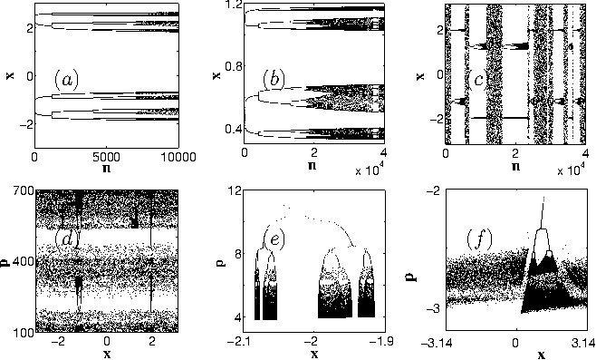
Figure 3: Attracting cascade of bifurcations type trajectories: (a) a single attracting trajectory of the standard Caputo fractional difference $\alpha$-family of maps with $\alpha=0.1$ and $K=2.41$; (b) a single attracting trajectory of the logistic Caputo $\alpha$-family of maps with $\alpha=0.1$ and $K=22.65$; (c) a single intermittent CBTT of the standard Riemann-Liouville $\alpha$-family of maps with $\alpha=1.65$ and $K=4.5$; (d) the phase space for the case (c); (e) a half of the attractor in the phase space of the standard Riemann-Liouville $\alpha$-family of maps with $\alpha=1.1$ and $K=3.5$; (f) CBTT (initial conditions $x_{0}=0$ and $p_{0}=-1.8855$) overlapping with a chaotic attractor (initial conditions $x_{0}=0$ and $p_{0}=-2.5135$) of the standard Caputo $\alpha$-family of maps with $\alpha=1.02$ and $K=4.5$.

One of the remarkable features of maps with power- asymptotically power-law memory is existence of attracting cascade of bifurcations type trajectories. Convergence to sinks of the period $T=2^{n}$ with $n>0$ may follow various scenarios. Trajectories may converge directly to a $T=2^{n}$ sink following a power law; they may initially converge to a sink of lower periodicity and then, through a few period doubling bifurcations converge to a $T=2^{n}$ sink; there is also a possibility (this way trajectories converge to attractors in Caputo $\alpha$-family of maps [39] with $1<\alpha<2$) that initially trajectories converge to a higher periodicity sink and then converge to a $T=2^{n}$ sink through a series of inverse bifurcations. Near the border with chaos (e.g., upper border of the area III in Fig. 1 (a)) the trajectories converge to CBTT. CBTT look like cascades of bifurcations in regular dynamics but bifurcations occur on a single attracting trajectory, Figs. 3 (a), (b), and (e), without any changes in maps’ memory ($\alpha$) or nonlinearity ($K$) parameters. Possible hidden symmetries in maps with power-law memory which lead to CBTT are not found yet. Another interesting phenomenon is intermittent CBTT (see Figs. 3 (c) and (d)) in which a trajectory may start as a chaotic trajectory, then converge to a periodic one, then turn back into a chaotic trajectory through a period doubling cascade of bifurcations, and this chain of transformations will repeat again and again. Existence of cascade of bifurcations type trajectories in phase spaces of systems with $1<\alpha<2$ is illustrated in Figs. 3 (e) and (f).

5 Conclusion

The results presented in this review are relevant to all natural and social systems with power-law memory. Let us mention a few possible areas of applications. In social sciences, the intermittent cascade of bifurcations evolution can be seen in evolution of systems on every level, starting from varying opinions of individuals and up to the evolution of a society as a whole. The history is a chain of repeating periods of democracy, chaos, and dictatorship.

The fact that in systems with power-law memory bifurcations depend on both nonlinearity and memory parameters may be particular interesting in medical application. As we mentioned in the introduction, almost each body organ’s tissues possess nonlinear viscoelastic properties and are nonlinear systems with power-law memory. There is even a Maple application Nonlinear Viscoelastic Behaviour of Brain Tissue (http://www.maplesoft.com/applications/view.aspx?SID=153923&view=html). If a disease is associated with changes in a nonlinearity parameter (whatsoever it is), then cure can be associated with changes in memory parameter (which could be associated with corrections in the nervous system). There are five types of surgical procedures to treat epilepsy. Each of them imposes changes in brain and correspondingly in memory. As the brain tissue is a nonlinear system with memory, one of the possible explanations of the success in the surgical treatment is that these changes in memory compensate for the abnormal value of the brain tissue nonlinearity parameter.

Definitely, all above mentioned systems are very complicated with many parameters, but in situations when one of the parameters is the most important to control the state of a system, nonlinear equations (maps or differential equations) with power-law memory can be used to model the system in order to explain and predict its evolution.

One of the basic tools in the analysis of nonlinear one-dimensional maps, the return map, makes no sense in the case of maps with memory, because the next value of a system variable $x_{n+1}$ depends on all previous values of this variable. The analysis of bifurcation diagrams in this case is quite complicated because individual trajectories may bifurcate and the rate of convergence to attracting points follows the power law $n^{-\alpha}$, which for small $\alpha$ typical for biological applications is very slow. The problem of finding some general form of self-similarity in maps with power-law memory is an open and important problem.

CBTT are found in discrete maps and to find them in continues systems described by fractional differential equations is another interesting problem. There are examples of continuous fractional chaotic systems of dimensions less than three but more than two. To prove impossibility of chaos in fractional continuous systems of lower dimensions or to find the counterexample is also an important open problem in the analysis of nonlinear systems with power-law memory.

References

- [1] F. Mainardi, Fractional Calculus and Waves in Linear Viscoelasticity: An Introduction to Mathematical Models (Imperial College Press, London, 2010).
- [2] V. E. Tarasov, Fractional Dynamics: Application of Fractional Calculus to Dynamics of Particles, Fields and Media (HEP, Springer, Berlin, 2010).
- [3] J. Klafter, S. C. Lim, and R. Metzler (Eds.), Fractional Dynamics: Recent Advances (World Scientific, Singapore, 2011).
- [4] I. Petras, Fractional-Order Nonlinear Systems (Springer, Berlin, 2011).
- [5] I. Nourdin, Selected Aspects of Fractional Brownian Motion (Springer, New York, 2013).
- [6] G. M. Zaslavsky, Hamiltonian Chaos and Fractional Dynamics (Oxford University Press, Oxford, 2008).
- [7] N. Laskin and G. M. Zaslavsky, Nonlinear fractional dynamics on a lattice with long-range interactions, Physica A 368, 38 (2006).
- [8] G. M. Zaslavsky, M. Edelman, and V. E. Tarasov, Dynamics of the chain of forced oscillators with long-range interaction: From synchronization to chaos, Chaos 17, 043124 (2007).
- [9] A. C. J. Luo and V. Afraimovich (Eds.), Long-range Interaction, Stochasticity and Fractional Dynamics (Springer, New York, 2010).
- [10] V. E. Tarasov, Fractional integro-differential equations for electromagnetic waves in dielectric media, Theor. and Math. Phys., 158, 355 (2009).
- [11] M. Caputo and F. Mainardi, Linear models of dissipation in anelastic solids, Rivista del Nuovo Cimento 1, 161 (1971).
- [12] M. Caputo and F. Mainardi, A new dissipation model based on memory mechanism, Pure and Applied Geophysics 91, 134 (1971).
- [13] V. E. Tarasov, Fractional gradient elasticity from spatial dispersion law, ISRN Condensed Matter Physics 2014, 794097 (2014).
- [14] A. Wineman, Nonlinear viscoelastic membranes, Computers and Mathematics with Applications 53, 168 (2007).
- [15] F. Prieur, G. Vilenskiy, and S. Holm, A more fundamental approach to the derivation of nonlinear acoustic wave equations with fractional loss operators, Journal of the Acoustical Society of America 132, 2169 (2012).
- [16] M. Edelman, Fractional Maps as Maps with Power-Law Memory, in Nonlinear Dynamics and Complexity; Series: Nonlinear Systems and Complexity, eds.: A. Afraimovich, A. C. J. Luo, and X. Fu (New York, Springer, 2014) pp. 79–120.
- [17] B. N. Lundstrom, M. H. Higgs, W. J. Spain, and A. L. Fairhall, Fractional differentiation by neocortical pyramidal neurons, Nature Neuroscience 11, 1335 (2008).
- [18] B. N. Lundstrom, A. L. Fairhall, and M. Maravall, Multiple time scale encoding of slowly varying whisker stimulus envelope incortical and thalamic neurons in vivo, J. Neuroscience 30, 5071 (2010).
- [19] A. L. Fairhall, G. D. Lewen, W. Bialek, and R. R. de Ruyter van Steveninck, Efficiency and Ambiguity in an Adaptive Neural Code, Nature 412, 787 (2001).
- [20] M. J. Kahana, Foundations of human memory (Oxford University Press, New York, 2012).
- [21] J. T. Wixted and E. Ebbesen, Genuine power curves in forgetting, Memory & Cognition 25, 731 (1997).
- [22] J. R. Anderson, Learning and memory: An integrated approach (Wiley, New York, 1995).
- [23] M. Edelman, Fractional Maps and Fractional Attractors. Part I: -Families of Maps, Discontinuity, Nonlinearity, and Complexity 1, 305 (2013).
- [24] R. M. May, Simple mathematical models with very complicated dynamics, Nature 261, 459 (1976).
- [25] E. Fick, M, Fick, and G. Hausmann, Logistic equation with memory, Physical Review A 44, 2469 (1991).
- [26] A. Fulinski and A. S. Kleczkowski, Nonlinear maps with memory, Physica Scripta 335, 119 (1987).
- [27] K. Hartwich and E. Fick, Hopf bifurcations in the logistic map with oscillating memory, Physics Letters A 177, 305 (1993).
- [28] M. Giona, Dynamics and relaxation properties of complex systems with memory, Nonlinearity 4, 911 (1991).
- [29] J. A. C. Gallas, Simulating memory effects with discrete dynamical systems, Physica A 195, 417 (1993); (198, 339 (1993) (erratum)).
- [30] A. A. Stanislavsky, Long-term memory contribution as applied to the motion of discrete dynamical system, Chaos 16, 043105 (2006).
- [31] M. Edelman, On Fractional Eulerian Numbers and Equivalence of Maps with Long-Range Power-Law Memory (Integral Volterra Equations of the Second Kind) to Grnvald-Letnikov Fractional Difference (Differential) Equations, Chaos 25, 073103 (2015).
- [32] I. Podlubny, Fractional Differential Equations (Academic Press, San Diego, 1999).
- [33] S. G Samko, A. A. Kilbas, and O. I. Marichev, Fractional Integrals and Derivatives Theory and Applications (Gordon and Breach, New York, 1993).
- [34] P. L. Butzer and M. Hauss, Eulerian numbers with fractional order parameters, Aequationes Mathematicae 46, 119 (1993).
- [35] A. A. Kilbas, H. M. Srivastava, and J. J. Trujillo, Theory and Application of Fractional Differential Equations (Elsevier, Amsterdam, 2006).
- [36] V. E. Tarasov and G. M. Zaslavsky, Fractional equations of kicked systems and discrete maps, J. Phys. A 41, 435101 (2008).
- [37] V. E. Tarasov, Discrete map with memory from fractional differential equation of arbitrary positive order, J. Math. Phys. 50 ,122703 (2009).
- [38] V. E. Tarasov, Differential equations with fractional derivative and universal map with memory, J. Phys. A 42, 465102 (2009).
- [39] M. Edelman, Universal Fractional Maps and Cascade of Bifurcations Type Attractors, Chaos 23, 033127 (2013).
- [40] M. Edelman, Caputo standard -family of maps: Fractional difference vs. fractional, Chaos 24, 023137 (2014).
- [41] M. Edelman, Fractional Maps and Fractional Attractors. Part II: Fractional Difference -Families of Maps, Discontinuity, Nonlinearity, and Complexity 4, 391 (2015).
- [42] M. Edelman and V. E. Tarasov, Fractional standard map, Phys. Let. A 374, 279 (2009).
- [43] M. Edelman, Universality in fractional dynamics, International Conference on Fractional Differentiation and Its Applications (ICFDA), 2014, DOI: 10.1109/ICFDA.2014.6967376, 1, (2014).
- [44] V. E. Tarasov and M. Edelman, Fractional dissipative standard map, Chaos 20, 023127 (2010).
- [45] M. Edelman, Fractional Standard Map: Riemann-Liouville vs. Caputo, Commun. Nonlin. Sci. Numer. Simul. 16, 4573 (2011).
- [46] M. Edelman, L. A. Taieb, New types of solutions of non-linear fractional differential equations, in: Advances in Harmonic Analysis and Operator Theory; Series: Operator Theory: Advances and Applications; A. Almeida, L. Castro, and F.-O. Speck (Eds.); pp. 139-155 (Springer, Basel, 2013).
- [47] G.-C. Wu, D. Baleanu, and S.-D. Zeng, Discrete chaos in fractional sine and standard maps, Phys. Lett. A 378, 484 (2014).