The most widely studied scenario in dark matter phenomenology is the thermal WIMP scenario. Inspite of numerous efforts to detect WIMP, till now we have no direct evidence for it. A possible explanation for this non-observation of dark matter could be because of its very feeble interaction strength and hence, failing to thermalise with the rest of the cosmic soup. In other words, the dark matter might be of non-thermal origin where the relic density is obtained by the so-called freeze-in mechanism. Furthermore, if this non-thermal dark matter is itself produced substantially from the decay of another non-thermal mother particle, then their distribution functions may differ in both size and shape from the usual equilibrium distribution function. In this work, we have studied such a non-thermal (fermionic) dark matter scenario in the light of a new type of ${\rm U}(1)_{\rm B-L}$ model. The ${\rm U}(1)_{\rm B-L}$ model is interesting, since, besides being anomaly free, it can give rise to neutrino mass by Type II see-saw mechanism. Moreover, as we will show, it can accommodate a non-thermal fermionic dark matter as well. Starting from the collision terms, we have calculated the momentum distribution function for the dark matter by solving a coupled system of Boltzmann equations. We then used it to calculate the final relic abundance, as well as other relevant physical quantities. We have also compared our result with that obtained from solving the usual Boltzmann (or rate) equations directly in terms of comoving number density, $Y$. Our findings suggest that the latter approximation is valid only in cases where the system under study is close to equilibrium, and hence should be used with caution.

1 Introduction

With the discovery of the flat rotation curves a few decades back [1], there was no doubt about the presence of dark matter in the Universe. From the recent observations of Planck [2], the existence of this mysterious dark matter has become even more certain. Their results also indicate a huge triumph of the $\Lambda$CDM cosmology where theory and experiments match to a great degree of accuracy. But unfortunately, all these predictions about the existence of dark matter were through indirect methods, mostly exploiting the gravitational interaction of the dark matter (for e.g. the detection of dark matter through the observation of flat rotation curves, or through gravitational lensing). Nothing much can be said about the particle nature of the dark matter, for e.g. whether it is a scalar or a fermion, what type of interaction it has with the Standard Model (SM) particles (if any at all), what is the strength of these type of interactions etc. For example dark matter mass can vary from $10^{-15}-10^{15}$ GeV, while its scattering cross section to SM particles ranges from $10^{-76}-10^{-41}$ cm² [3]. This has led to many scientifically motivated speculations about its nature. A very interesting scenario is the WIMP (Weakly Interacting Massive Particles), where dark matter particles interact with the weak interaction strength and is simultaneously able to satisfy the relic density constraint. These are thermal relics, which remained in the Universe as dark matter particles after the process of thermal freeze-out [4, 5]. From the direct detection point of view, we also have very little success. Non-observations from the recent direct detection experiments [6, 7], have put a strong upper bound on the dark matter-nucleon interaction cross section. Future experiments [8, 9] will make this limit even stronger. With the increasing sensitivity of these direct detection experiments, the dark matter nucleon cross section can become as low as the neutrino-nucleon elastic scattering cross section [10]. So in a few years time, we are going to be in the era where we can not distinguish a dark matter signal from that of a neutrino. Only possible way of distinguishing the two will then be directional searches [11]. Another alternative idea to explore is to go beyond the thermal scenario, and assume that the dark matter is even more weakly interacting than the WIMPs (hence explaining the null result in the direct detection experiments) and consequently has never been able to attain thermal equilibrium. The relic density is obtained through freeze-in scenario [12]. Many models that explains the relic density through this type of mechanism have been studied in detail in Refs. [12, 13, 14, 15, 16, 17, 18, 19]. Earlier works however had already focussed on the production mechanism of lighter states from decays of heavier parent particles in the early Universe [20, 21]. For example, sterile neutrino production from the decay of heavier particles have been discussed in Refs. [22, 23, 24]. Approximate analytical solutions for non-thermal dark matter production from decays can be found in Ref. [25].

In this work we studied the viability of a non-thermal dark matter candidate within the framework of a recently proposed model called the new ${\rm U}(1)_{\rm B-L}$ model [26]. It is new in the sense that this model unlike the usual ${\rm U}(1)_{\rm B-L}$ model has no right handed neutrinos. Four chiral fermions are however introduced for anomaly cancellations. These chiral fermions linearly combine together in mass basis to give rise to two Dirac fermions namely $\psi_{1}$ and $\psi_{2}$. Two extra scalars were introduced in order to give masses to these fermions. The charge assignment of the new particles under the ${\rm U}(1)_{\rm B-L}$ gauge group is consequently different from the usual model. Since the model is symmetric under a local gauge group (i.e. ${\rm U}(1)_{\rm B-L}$), it naturally has an extra gauge boson ($Z_{\rm BL}$), which gets mass after this extra gauge symmetry is broken spontaneously. We will take the lightest of the two Dirac fermions ($\psi_{1}$) as our non-thermal dark matter candidate.

Another novel feature of this new model (as was already noted in [26]) is that it can explain the generation of neutrino mass through a Type II see-saw mechanism upon the introduction of a new scalar triplet ($\Delta$) with suitable B-L charge.

The study assuming the lightest Dirac fermion to be a thermal dark matter has already been done in Ref. [26]. We see from their analysis that the relic density constraint is actually satisfied within very small regions. It is satisfied either when $M_{DM}\sim M_{Z_{\rm BL}}/2$ (i.e. near the resonance) or when dark matter mass is $\sim 4$ TeV. But a priori there is no reason for the dark matter mass to be $\sim M_{Z_{\rm BL}}/2$ as there is no symmetry in the Lagrangian, which can relate the masses of dark matter ($\psi_{1}$) and $Z_{\rm BL}$ in the above mentioned way. This naturally motivates one to study the implications of a non-thermal dark matter candidate within this frame work. Imposing the non-thermality condition implies that unlike in the thermal case, the dark matter particles are so feebly interacting that they never attain thermal equilibrium. An approximate mathematical statement in this regard will be $\frac{n_{eq}\langle\sigma v\rangle}{H}<1$, which means that the interaction rate for scattering of dark matter particles is less than the expansion rate of the Universe and hence the particles fail to scatter with other particles within the thermal plasma and so remains out of the thermal soup. We have shown in this work that, this model can indeed accommodate a non-thermal dark matter candidate with correct relic density. We have solved a coupled set of Boltzmann equations to find the momentum distribution function for the dark matter particles. Knowledge of the non-equilibrium momentum distribution function (unlike in the usual scenarios where only the comoving number density ($Y=n/s$) is solved for) will allow us to calculate all the relevant quantities of interest like the relic density (from freeze in), constraints from structure formation, bounds from relativistic degrees of freedom etc. It is well known that, if the particles under consideration are produced from a non-thermal source (e.g. from the decay of an out of equilibrium mother particle) then solving the usual Boltzmann equations in terms of $Y$ is only an approximate method to find the comoving number density. This formalism will provide roughly the correct result as long as we do not move far from equilibrium. In light of this, we have also discussed and compared results from our exact calculations with that obtained from the above mentioned approximate method.

An important difference with the earlier work is that unlike in [26], here all the (three) mixing angles between the three scalars (i.e. SM Higgs, and the two non-standard Higgs) are taken into account and we have found that in some cases, two of them significantly control the final DM abundance.

The rest of the work is divided as follows: In Section 2 we have elaborately discussed about the new ${\rm U}(1)_{\rm B-L}$ model. Section 3 deals with the FIMP scenario and also with the coupled Boltzmann equations needed to solve the non-thermal momentum distribution function of DM. The results that we have found by solving the coupled Boltzmann equations are presented in Section 4. In Section 5 we discuss about the relevant theoretical as well as experimental constraints on this non-thermal dark matter scenario. Finally the conclusion is given Section 6. The detailed derivations all the collision terms as well as the relevant vertex factors and decay widths are given in the Appendix.

2 A new U(1)_B-L extension of Standard Model

We consider a new ${\rm U}(1)_{\rm B-L}$ extension of the Standard Model of particle physics. The model has been proposed in Ref. [26]. This model does not contain any sterile neutrino like the minimal ${\rm U}(1)_{\rm B-L}$ model [27] which is usually studied in the literature. The gauge group however is the same i.e. ${\rm SU}(2)_{\rm L}\times{\rm U}(1)_{\rm Y}\times{\rm U}(1)_{\rm B-L}$. But in the absence of the three sterile neutrinos we need some extra chiral fermions for the cancellation of axial vector anomaly [28] and mixed gravitational-gauge anomaly [29]. Hence four chiral fermions namely $\zeta$, $\eta_{L}$, ${\chi_{1}}_{R}$ and ${\chi_{2}}_{R}$ with suitable ${\rm B-L}$ charges are introduced. In order to generate Dirac type mass terms for these chiral fermions in a gauge invariant manner we need two distinct scalar fields ($\phi_{1}$, $\phi_{2}$) with different ${\rm B-L}$ charges. All the fields and their corresponding charges under ${\rm SU}(2)_{\rm L}$, ${\rm U}(1)_{\rm Y}$ and ${\rm U}(1)_{\rm B-L}$ gauge groups are given in Table 1. The presence of a new gauge symmetry (${\rm U}(1)_{\rm B-L}$) also introduces its corresponding gauge boson ($Z_{\rm BL}$) to the particle spectrum and $Z_{\rm BL}$ becomes massive whenever the proposed ${\rm B-L}$ symmetry is broken spontaneously by the VEVs of scalar fields.

	Field	$\boldsymbol{{\rm SU(2)_{L}}}$	$\boldsymbol{{\rm U(1)_{Y}}}$	$\boldsymbol{{\rm U}(1)_{\rm B-L}}$	VEV
		charge	charge	charge
	$l_{\rm L}\equiv(\nu_{\rm L}\,\,\,\,e_{\rm L})^{\rm T}$	2	-$\frac{1}{2}$	-1
	$Q_{\rm L}\equiv(u_{\rm L}\,\,\,\,d_{\rm L})^{\rm T}$	2	$\frac{1}{6}$	$\frac{1}{3}$
SM Fermions	$e_{\rm R}$	1	-$1$	-1	0
	$u_{\rm R}$	1	$\frac{2}{3}$	$\frac{1}{3}$
	$d_{\rm R}$	1	-$\frac{1}{3}$	$\frac{1}{3}$
	$\xi_{\rm L}$	1	0	$\frac{4}{3}$
BSM Fermions	$\eta_{\rm L}$	1	0	$\frac{1}{3}$	0
	${\chi_{1}}_{\rm R}$	1	0	$-\frac{2}{3}$
	${\chi_{2}}_{\rm R}$	1	0	$-\frac{2}{3}$
	$H$	2	$\frac{1}{2}$	0	$v$
Scalars	$\phi_{1}$	1	$0$	$1$	${v_{1}}$
	$\phi_{2}$	1	$0$	$2$	${v_{2}}$
	$\Delta$	3	$1$	$-2$	${v_{t}}$

Table 1: ${\rm SU}(2)_{\rm L}$, ${\rm U}(1)_{\rm Y}$ and ${\rm U}(1)_{\rm B-L}$ charges and corresponding VEVs of all the fields involved in the present model.

The gauge invariant Lagrangian for these new fields is given by:

$$\mathscr{L}_{\rm BL} = i\,\overline{\eta_{\rm L}}\,\gamma_{\mu}\,D^{\mu}_{\eta}\,\eta_{\rm L}+i\,\overline{\xi_{\rm L}}\,\gamma_{\mu}\,D^{\mu}_{\xi}\,\xi_{\rm L}+i\sum_{i=1}^{2}\,\overline{{{\chi}_{i}}_{\rm R}}\,\gamma_{\mu}\,D^{\mu}_{\chi_{i}}\,{{\chi}_{i}}_{\rm R}-\frac{1}{4}F_{Z_{\rm BL}}^{\mu\nu}{F_{Z_{\rm BL}}}_{\,\mu\nu}$$ (1)

$$+\sum_{i=1}^{2}(D^{\mu}_{\phi_{i}}\phi_{i})^{\dagger}({D_{\phi_{i}}}_{\mu}\phi_{i})-\sum_{i=1}^{2}\left({y_{\xi}}_{i}\,\overline{\xi_{\rm L}}\,{\chi_{i}}_{\rm R}\,\phi_{2}+{y_{\eta}}_{i}\,\overline{\eta_{\rm L}}\,{\chi_{i}}_{\rm R}\,\phi_{1}+h.c.\,\right)$$

$$-\,V(H,\,\phi_{1},\,\phi_{2})+\mathscr{L}_{\Delta}\,,$$

where ${D_{\psi}}_{\mu}$ is the covariant derivative for the field $\psi$ ($\psi=\eta_{\rm L},\,\xi_{\rm L},\,{\chi_{i}}_{\rm R}$ and $\phi_{i}$). General expression of ${D_{\psi}}_{\mu}$ for a field $\psi$ with a ${\rm B-L}$ charge $Q_{\rm B-L}(\psi)$ is given by

$${D_{\psi}}_{\mu}=\left({\partial}_{\mu}+i\,Q_{\rm BL}(\psi)\,g_{\rm BL}\,{Z_{\rm BL}}_{\mu}\gamma^{\mu}\right)\,.$$

Here $g_{\rm BL}$ is the new gauge coupling corresponding to the gauge group ${\rm U}(1)_{\rm B-L}$ while $F_{Z_{\rm BL}}^{\mu\nu}$ is the usual field tensor of the new gauge boson $Z_{\rm BL}$. The Yukawa couplings of the chiral fermions are denoted by ${y_{\xi}}_{i}$ and ${y_{\eta}}_{i}$. These chiral fermions $\eta_{\rm L},\,\xi_{\rm L},\,{\chi_{1}}_{\rm R}$ and ${\chi_{2}}_{\rm R}$ in gauge basis do not represent any physical fermionic field. In mass basis, they combine together to give rise new physical states $\psi_{1}$ and $\psi_{2}$ with masses $M_{\psi_{1}}$ and $M_{\psi_{2}}$ respectively. The scalar potential including all possible gauge invariant as well as renormalisable interaction terms among $H$, $\phi_{1}$ and $\phi_{2}$ is given by:

$$V(H,\phi_{1},\phi_{2}) = \mu^{2}_{H}H^{\dagger}H+\lambda_{H}(H^{\dagger}H)^{2}+\mu^{2}_{1}\phi^{\dagger}_{1}\phi_{1}+\lambda_{1}(\phi^{\dagger}_{1}\phi_{1})^{2}+\mu^{2}_{2}\phi^{\dagger}_{2}\phi_{2}+\lambda_{2}(\phi^{\dagger}_{2}\phi_{2})^{2}$$ (2)

$$+\rho_{1}(H^{\dagger}H)(\phi^{\dagger}_{1}\phi_{1})+\rho_{2}(H^{\dagger}H)(\phi^{\dagger}_{2}\phi_{2})+\lambda_{3}(\phi^{\dagger}_{1}\phi_{1})(\phi^{\dagger}_{2}\phi_{2})$$

$$+\mu\left(\phi_{2}\phi^{\dagger^{2}}_{1}+\phi_{2}^{\dagger}\phi^{{}^{2}}_{1}\right)\,,$$

where $H$ is the usual Standard Model Higgs doublet, while $\phi_{1}$ and $\phi_{2}$ are the new scalars which are required to generate fermion masses in a gauge invariant way after symmetry breaking. The ${\rm U}(1)_{\rm B-L}$ symmetry is assumed to be broken spontaneously above the electroweak phase transition scale. The scalar potential defined above should be bounded from below. In other words, it should have stable minima. The existence of a stable minimum of the potential puts some conditions on the quartic couplings. These are known as the vacuum stability condition, and are given by:

$$\lambda_{H},\,\,\lambda_{1},\,\,\lambda_{2} \geq 0\,,$$

$$\rho_{1}+\sqrt{\lambda_{H}\lambda_{1}} \geq 0\,,$$

$$\rho_{2}+\sqrt{\lambda_{H}\lambda_{2}} \geq 0\,,$$

$$\lambda_{3}+\sqrt{\lambda_{1}\lambda_{2}} \geq 0\,,$$ (3)

and

$$\sqrt{\lambda_{H}\,\lambda_{1}\,\lambda_{2}}+\rho_{1}\,\sqrt{\lambda_{2}}+\rho_{2}\,\sqrt{\lambda_{1}}+\lambda_{3}\,\sqrt{\lambda_{H}}+$$

$$\sqrt{2(\rho_{1}+\sqrt{\lambda_{H}\lambda_{1}})\,(\rho_{2}+\sqrt{\lambda_{H}\lambda_{2}})\,(\lambda_{3}+\sqrt{\lambda_{1}\lambda_{2}})}\geq 0\,.$$ (4)

The neutral component of the Higgs doublet ($H^{0}$) and the other two scalars acquire VEVs after symmetry breaking:

$$H^{0} = \frac{1}{\sqrt{2}}(v+\tilde{h})+\frac{i}{\sqrt{2}}\tilde{G}\,,$$

$$\phi_{1} = \frac{1}{\sqrt{2}}(v_{1}+\tilde{h}_{1})+\frac{i}{\sqrt{2}}\tilde{A}_{1}\,,$$

$$\phi_{2} = \frac{1}{\sqrt{2}}(v_{2}+\tilde{h}_{2})+\frac{i}{\sqrt{2}}\tilde{A}_{2}\,,$$ (5)

where $v$, $v_{1}$ and $v_{2}$ are the respective VEVs, $\tilde{h}$, $\tilde{h}_{1}$ and $\tilde{h}_{2}$ are the CP-even scalars, while $\tilde{G}$, $\tilde{A}_{1}$ and $\tilde{A}_{2}$ are the CP-odd counterparts. From the minimisation condition, i.e. equating the first order derivative of the scalar potential $V(H,\,\phi_{1},\,\phi_{2})$ to zero with respect to each of the scalars, we get the following equations:

$$\mu^{2}_{H} = -\left(\lambda_{H}v^{2}+\frac{\rho_{1}}{2}v^{2}_{1}+\frac{\rho_{2}}{2}v^{2}_{2}\right),$$

$$\mu^{2}_{1} = -\left(\lambda_{1}v^{2}_{1}+\frac{\rho_{1}}{2}v^{2}+\frac{\lambda_{3}}{2}v^{2}_{2}+\sqrt{2}v_{2}\,\mu\right)\,,$$

$$\mu^{2}_{2} = -\left(\lambda_{2}v^{2}_{2}+\frac{\rho_{2}}{2}v^{2}+\frac{\lambda_{3}}{2}v^{2}_{1}+\frac{1}{\sqrt{2}}\dfrac{v^{2}_{1}\,\mu}{v_{2}}\right).$$ (6)

After the spontaneous breaking of all the gauge symmetries that we have imposed on the model Lagrangian (Eq. (1)), three CP-even scalars ($\tilde{h}$, $\tilde{h}_{1}$, $\tilde{h}_{2}$) mix among themselves. With respect to the basis states $\tilde{h}$-$\tilde{h}_{1}$-$\tilde{h}_{2}$ (gauge basis), the mass matrix of the CP-even scalars is given by

$$\mathscr{M}^{2}_{\rm CP\,even}=\begin{pmatrix}2\lambda_{H}v^{2}&\rho_{1}v\,v_{1}&\rho_{2}v\,v_{2}\\ \rho_{1}v\,v_{1}&2\lambda_{1}v_{1}^{2}&(\lambda_{3}v_{2}+\sqrt{2}\mu)\,v_{1}\\ \rho_{2}v\,v_{2}&(\lambda_{3}v_{2}+\sqrt{2}\,\mu)\,v_{1}&(2\lambda_{2}v_{2}^{2}-\frac{\mu\,v_{1}^{2}}{\sqrt{2}\,v_{2}})\end{pmatrix}\,.$$ (7)

It should be noted that, while deriving the mass matrix, we have used the conditions obtained from extremising the scalar potential i.e. Eq. (6). Now, in order to find the physical scalar states and their respective masses we have to find a new basis states ($h_{1}$, $h_{2}$, $h_{3}$) with respect to which the above mass matrix becomes diagonal. This new basis states are known as the mass basis. As in this case, the CP-even scalars mass matrix is a real symmetric one (assuming all the parameters in the Lagrangian are real), the gauge basis and mass basis states must be related by an orthogonal matrix which is the PMNS matrix with zero complex phase. The three mixing angles are $\theta_{12},\,\theta_{13},\,\theta_{23}$. So we have:

$$\mathscr{U}_{\rm PMNS}(\theta_{12},\,\theta_{23},\,\theta_{13})=$$

$$\begin{pmatrix}\cos\theta_{12}\cos\theta_{13}&\sin\theta_{12}\cos\theta_{13}&\sin\theta_{13}\\ -\sin\theta_{12}\cos\theta_{23}-\cos\theta_{12}\sin\theta_{23}\sin\theta_{13}&\cos\theta_{12}\cos\theta_{23}-\sin\theta_{12}\sin\theta_{23}\sin\theta_{13}&\sin\theta_{23}\cos\theta_{13}\\ \sin\theta_{12}\sin\theta_{23}-\cos\theta_{12}\cos\theta_{23}\sin\theta_{13}&-\cos\theta_{12}\sin\theta_{23}-\sin\theta_{12}\cos\theta_{23}\sin\theta_{13}&\cos\theta_{23}\cos\theta_{13}\end{pmatrix}\,,$$

and hence the gauge basis and the mass basis states are related by:

$$\begin{pmatrix}h_{1}\\ h_{2}\\ h_{3}\end{pmatrix}=\mathscr{U}_{\rm PMNS}(\theta_{12},\,\theta_{23},\,\theta_{13})\begin{pmatrix}\tilde{h}\\ \tilde{h}_{1}\\ \tilde{h}_{2}\end{pmatrix}\,.$$ (8)

Like the the CP-even scalar sector, the CP odd sector also exhibits mixing between the pseudo scalars. However in this case, only the pseudo scalars ($\tilde{A}_{1}$, $\tilde{A}_{2}$) of the singlets $\phi_{1}$ and $\phi_{2}$ mix with each other. This is because the CP odd scalar ($\tilde{G}$) of the Higgs doublet $H$ does not mix with the CP odd portion of the other two complex scalars ($\phi_{1}$ and $\phi_{2}$), which are SU(2)_L singlets. This is due to the fact that with a doublet and a complex singlet scalar we cannot write a gauge invariant term in the Lagrangian and also all the VEVs are assumed to be real and associated with the CP even sector. Hence terms involving odd powers of $\tilde{G}$ is absent here. The CP odd scalars mixing matrix is thus given by:

$$\mathscr{M}^{2}_{CP-odd}=\sqrt{2}\,\begin{pmatrix}-\,2\mu\,v_{2}&\,\mu\,v_{1}\\ \mu\,v_{1}&-\,\frac{\mu\,v_{1}^{2}}{2\,v_{2}}\end{pmatrix}\,.$$ (9)

On diagonalisation we find that one of the eigenvalues of the matrix is zero as expected and which corresponds to a massless Goldstone mode. The mass of only physical pseudo scalar is given by:

$$M_{A}^{2}=-\frac{\mu\,v_{2}}{\sqrt{2}\,\beta^{2}}\left(1+4\,\beta^{2}\right)\,,$$ (10)

where $\beta=\dfrac{v_{2}}{v_{1}}$, the ratio of VEVs of $\phi_{2}$ and $\phi_{1}$. Since mass of this pseudo scalar is always positive, the above equation implies that $\mu<0$. Also in terms of the mixing angle $\alpha$ between $A_{1}$ and $A_{2}$, the expression of $M^{2}_{A}$ can also be written in the following form

$$M^{2}_{A}=-2\sqrt{2}\dfrac{\mu\,v_{2}}{\sin^{2}\alpha}$$ (11)

with mixing angle $\alpha=\tan^{-1}2\,\beta$.

The fermions in the present model also get masses after the spontaneous breaking of the ${\rm U}(1)_{\rm B-L}$ gauge symmetry. The masses of the fermions arise from the Yukawa interaction terms appearing in Eq. (1), when $\phi_{1}$ and $\phi_{2}$ get their VEVs. The Yukawa interaction terms involving only chiral fermions in Eq.  (1), can also be written in the following matrix form

$$\mathscr{L}_{\rm fermion-mass} = \left(\begin{array}[]{cc}\overline{\xi_{\rm L}}&\overline{\eta_{\rm L}}\end{array}\right)\mathscr{M}_{\rm fermion}\left(\begin{array}[]{c}{\chi_{1}}_{\rm R}\\ {\chi_{2}}_{\rm R}\end{array}\right)+h.c.,$$ (15)

where

$$\mathscr{M}_{\rm fermion} = \left(\begin{array}[]{cc}{y_{\xi}}_{1}v_{2}&{y_{\xi}}_{2}v_{2}\\ {y_{\eta}}_{1}v_{1}&{y_{\eta}}_{1}v_{1}\end{array}\right)$$ (18)

is the mass matrix for the chiral fermions, which can in general be diagonalised by a bi-unitary transformation. From the expression of mass matrix, one can notice that the $\mathscr{M}_{\rm fermion}$ is not a symmetric matrix (Dirac type). Hence in the mass basis we have two physical Dirac fermions ($\psi_{1}$ and $\psi_{2}$). The mass and gauge basis states are related by:

$$\begin{pmatrix}{\xi}_{\rm L}\\ {\eta}_{\rm L}\end{pmatrix}=\mathscr{U}_{\rm L}\begin{pmatrix}{\psi_{2}}_{\rm L}\\ {\psi_{1}}_{\rm L}\end{pmatrix},\qquad\begin{pmatrix}{\chi_{1}}_{\rm R}\\ {\chi_{2}}_{\rm R}\end{pmatrix}=\mathscr{U}_{\rm R}\begin{pmatrix}{\psi_{2}}_{\rm R}\\ {\psi_{1}}_{\rm R}\end{pmatrix}.$$ (19)

Where $\mathscr{U}_{\rm L,\,R}$ are two unitary matrices and for the case when all the Yukawa couplings (${y_{\xi}}_{i}$ and ${y_{\eta}}_{i}$) are real numbers, these matrices can be the usual $2\times 2$ rotation matrix. Therefore, for this case $\mathscr{U}_{\rm L,\,R}$ can be written as

$$\mathscr{U}_{\rm L,\,R}=\begin{pmatrix}\cos\theta_{\rm L,\,R}&\sin\theta_{\rm L,\,R}\\ -\sin\theta_{\rm L,\,R}&\cos\theta_{\rm L,\,R}\end{pmatrix}\,$$ (20)

with $\theta_{\rm L,\,R}$ are the respective mixing angles for the left chiral and the right chiral states. In the mass basis, the two physical fermionic states are $\psi_{1}={\psi_{1}}_{\rm L}+{\psi_{1}}_{\rm R}$, $\psi_{2}={\psi_{2}}_{\rm L}+{\psi_{2}}_{\rm R}$ and the lightest one would automatically be stable, hence can serve as a viable dark matter candidate. Without any loss of generality, throughout the present work, we assume the lightest fermion $\psi_{1}$ is our dark matter candidate.

The breaking of ${\rm U}(1)_{\rm B-L}$ symmetry, besides giving masses to the fermions also makes the extra gauge boson $Z_{\rm BL}$ massive. Its mass is given by :

$$M^{2}_{Z_{\rm BL}}=\left(\dfrac{g_{\rm BL}\,v_{2}}{\beta}\right)^{2}(1+4\beta^{2})\,.$$ (21)

The set of independent parameters relevant for our analysis are as follows:
$\theta_{12},\,\theta_{13},\,\theta_{23},\,\theta_{\rm L},\,\theta_{\rm R},\,M_{h_{2}},\,M_{h_{3}},\,M_{A},\,M_{\psi_{1}},\,M_{\psi_{2}},\,M_{Z_{\rm BL}},\,g_{\rm BL}$ and $\beta$. Other model parameters can be written in terms of all these independent variables. In addition, we have chosen $h_{1}$ as the SM-like Higgs boson which has recently been discovered by ATLAS [30], CMS [31] collaborations of LHC at CERN and consequently we have kept fixed $M_{h_{1}}$ and $v$ at 125.5 GeV and 246 GeV respectively. The relevant vertex factors (in terms of the independent parameters) that we will need in our further calculations of DM distribution function as well as its comoving number density, are given in the Appendix A.1.

As there are no right handed neutrinos in this new ${\rm U}(1)_{\rm B-L}$ model, which are usually present in ${\rm U}(1)_{\rm B-L}$ extended Standard Model to cancel gauge anomaly, light active neutrinos remain massless. We can overcome this situation by using Type-II see-saw mechanism [32, 33, 34] for which one has to introduce a scalar field $\Delta$ which is a triplet under SU$(2)_{\rm L}$. In Eq. (1) the term $\mathscr{L}_{\Delta}$ represents the Lagrangian for the triplet $\Delta$ field. The $\Delta$ field also has a ${\rm B-L}$ charge -2, which is required to write a gauge invariant Yukawa term involving $\Delta$ and two lepton doublet ($l_{\rm L}$) via $\mathscr{L}_{\Delta}\supset-{Y_{\nu}}_{{}_{\alpha\beta}}{l^{\rm T}_{\alpha}}_{\rm L}\,Ci\,\sigma_{2}\,\Delta\,{l_{\beta}}_{\rm L}$, where ${l_{\alpha}}_{\rm L}$ is the usual left handed lepton doublet of flavour $\alpha$ while $C$ is the charge conjugation matrix. Therefore, neutrinos become massive with ${m_{\nu}}_{ij}={Y_{\nu}}_{{}_{ij}}\,\dfrac{v_{t}}{\sqrt{2}}$, when the neutral component of $\Delta$ acquires a VEV $v_{t}$. However, the VEV of $\Delta$ field is related to that of SM Higgs doublet through the relation $v_{t}\sim\dfrac{\mu\,v^{2}}{\sqrt{2}\,M^{2}_{\Delta}}$ [35] (when $v>>v_{t}$, required for $\rho$ parameter to be equal to 1). Here $M^{2}_{\Delta}$ is the coefficient for the quadratic term (mass term) of $\Delta$ in the $\mathscr{L}_{\Delta}$ ($\supset-M^{2}_{\Delta}{\rm Tr}(\Delta^{\dagger}\Delta)$) while $\mu$ is the coefficient of the trilinear term between two Higgs doublets ($H$) and a $\Delta$. In our present case, such a trilinear interaction term is although forbidden, but can be generated from a term like $\lambda^{\prime}H^{\rm T}i\sigma_{2}\Delta^{\dagger}H\,\phi_{2}$ in a gauge invariant manner, when $\phi_{2}$ gets its VEV. Therefore in our case $\mu=\lambda^{\prime}\dfrac{v_{2}}{\sqrt{2}}$ and consequently ${m_{\nu}}_{{}_{ij}}={Y_{\nu}}_{{}_{ij}}\,\dfrac{\lambda^{\prime}\,v_{2}\,v^{2}}{2\sqrt{2}\,M^{2}_{\Delta}}$. Hence, in order to produce neutrino masses $\sim\mathcal{O}(0.1)$ eV, we need $M_{\Delta}\sim 10^{8}$ GeV for $Y_{\nu}\sim 10^{-1}$ and $\lambda^{\prime}\,v_{2}\sim 1$ TeV (possible as we have assumed before that the ${\rm B-L}$ symmetry breaking occurs well above the EWPT). As a results the masses of the scalar fields within the triplet $\Delta$ will be several orders of magnitude higher than those of particles we are considering in this work. Hence the effect of the formers will be negligibly small at that epoch of the Universe (Temperature $\leq 10$ TeV) where we have done our analysis.

3 The FIMP paradigm

Now we turn to the problem of investigating a non-thermal fermionic dark matter candidate ($\psi_{1}$) within the framework of this new ${\rm U}(1)_{\rm B-L}$ model. As already discussed before, since the thermal scenario is only viable either near the resonance, or near the high mass range where mass of dark matter $\sim\mathcal{O}\,(4\,\rm TeV)$, hunt for a non-thermal dark matter candidate is quite natural. In the usual scenario (i.e. the thermal scenario), dark matter has weak but sizeable interaction with other particles in the thermal plasma. But as the Universe evolves it freezes out and drops out of the thermal bath. Freeze-out occurs because the rate of collision of DM particles falls below the expansion rate after a certain time, and the dark matter species retains its value of comoving number density at the freeze out temperature. But situations may be such that from the very beginning dark matter particles are so very weakly interacting with the particles in the thermal soup, that they never enter thermal equilibrium in the first place. So their initial number density is almost negligible. But as the Universe evolves, these may begin to be produced (mostly from the decays of) heavier mother particle(s). In the case where the mother particles are in thermal equilibrium, the production of these non-thermal dark matter particles is most significant at around $T_{\rm Universe}\sim M$, where $M$ is the mass of the mother particle. So, starting from a negligible initial number density, the number density of the dark matter particles will increase and may finally evolve to match the relic density constraint. Moreover, there can be a situation when the mother particles are not even in equilibrium. Then we will also have to solve the momentum distribution function for the mother particle as well. This, (as we will see here) leads to a coupled set of Boltzmann equations. Since the initial number density of these non-thermal dark matter is extremely small, inverse reactions are often neglected while solving the Boltzmann equations [36, 37]. Since the dominant production mode of a non-thermal dark matter is the decay of heavy particles at the early epoch, the condition for non-thermality is given by $\dfrac{\Gamma}{H}<1\biggm{\lvert}_{T\sim M}$ [38], where $H$ is the Hubble parameter, $M$ is the mass of the decaying mother particle while $\Gamma$ is the corresponding decay width. This gives an order of magnitude estimate (upper bound) of the coupling strength needed for a species remains out of equilibrium in the early Universe. Using the non-thermality criterion we find that for a decaying particle of mass $\mathcal{O}$(TeV), the extra gauge coupling $g_{\rm BL}$ must be less than $10^{-7}$.

Most of the earlier studies involving calculation of DM relic abundance have attempted to solve the Boltzmann equation in terms of the comoving number density $Y=\dfrac{n}{s}$ of the relic particle. But this approach is valid as long as the decaying and the annihilating particles (except one whose comoving number density is being solved) are in thermal equilibrium or at least their distribution functions are similar in shape to the equilibrium distribution function and do not vary much from the latter. However this situation is certainly not guaranteed here, since one of the decaying particles ($Z_{\rm BL}$) is not in equilibrium. Thus in order to compute the DM relic density, first we need to calculate the momentum distribution function of $Z_{\rm BL}$ followed by that of $\psi_{1}$. Hence, we have solved a set of coupled Boltzmann equations at the level of momentum distribution functions for each of $Z_{\rm BL}$ and $\psi_{1}$ (other decaying particles are assumed to be in thermal equilibrium) following Ref. [39]. Once we have the knowledge about both the distribution functions, it is straight forward to calculate the other physical quantities like comoving number density, relic density etc.

3.1 Coupled Boltzmann equations and its solution

The Boltzmann equation for the distribution function $f(p)$, in its most general form can be written in terms of the Liouville operator ($\hat{L}$) and the collision term ($\mathcal{C}$). Symbolically, it is written as:

$$\hat{L}\,f=\mathcal{C}[f]\,.$$

For an isotropic and homogeneous Universe, using the FRW metric we find that $\hat{L}=\frac{\partial}{\partial t}-Hp\frac{\partial}{\partial p}$, where $p=\lvert\vec{p}\rvert$ is the absolute value of the particle’s three momentum. As in Ref. [39] making the transformation of variable:

$$r = \frac{M_{sc}}{T}\,,$$ (22)

$$\xi_{p} = \Bigg{(}\frac{g_{s}(T_{0})}{g_{s}(T)}\Bigg{)}^{1/3}\frac{p}{T}\,,$$ (23)

where $M_{sc}$ and $T_{0}$ are some reference mass scale and temperature respectively, we find that the Liouville operator takes the following form:

$$\hat{L} = rH\Bigg{(}1+\frac{T\,g_{s}^{\prime}}{3\,g_{s}}\Bigg{)}^{-1}\frac{\partial}{\partial r}\,,$$ (24)

where $g_{s}(T)$ is the effective number of degrees of freedom related to the entropy density of the Universe while $g_{s}^{\prime}$ denotes differentiation of $g_{s}$ with respect to temperature $T$. The form of the function $g_{s}\,(T)$ is taken from Ref. [5] (Fig. 1). The bulk of the contribution to the effective degrees of freedom ($g_{s}$) comes from the relativistic (SM) particles in equilibrium with the thermal soup  . The reference mass scale $M_{sc}$ is taken to be the mass of the Standard Model Higgs boson ($M_{h_{1}}$) throughout the rest of the work.

The main production channels for the non-thermal dark matter $\psi_{1}$ are from the decays of $h_{1},\,h_{2}$ and $Z_{\rm BL}$. All of these BSM particles have been assumed to have mass of $\sim\mathcal{O}$(TeV). Among the three decaying particles, $Z_{\rm BL}$ is itself very feebly interacting (due to very low value of $g_{\rm BL}$) and remains outside the thermal soup. The BSM scalar $h_{2}$ can be in thermal equilibrium, as it can interact with the SM particles through its mixing with $h_{1}$, which need not be too small even in the non-thermal scenario. In whole of the analysis that will follow, (for simplicity) we have assumed that the CP odd scalar $A$, the extra fermion $\psi_{1}$ and one of the three CP even scalars (say $h_{3}$) are much heavier than rest of the particles and hence they have negligible abundance during the epoch of interest here (due to exponential Boltzmann suppression). So the production of dark matter particles from these very heavy states can safely be neglected since there are almost no particles left in the thermal bath to produce $\psi_{1}$. So, $\psi_{1}$ is partly produced from the decay of $h_{1}$ and $h_{2}$ which are in thermal equilibrium, and consequently the usual equilibrium Boltzmann distribution function has been assumed for them. $\psi_{1}$ is also produced from the decay of $Z_{\rm BL}$ which is out of equilibrium, and hence we have to solve for its non-equilibrium distribution function separately. Hence we have to solve two coupled Boltzmann equations. From the first one we calculate the non-equilibrium momentum distribution function of $Z_{\rm BL}$. This solution is then used in the second equation to find the final non-equilibrium momentum distribution function of $\psi_{1}$. The scattering terms contribute very little in the freeze-in scenario and hence left out in rest of the analysis [18, 37]. The coupled set of Boltzmann equations necessary for calculating the momentum distribution function of $\psi_{1}$ are as follows:

$$\,\,\hat{L}\,f_{Z_{\rm BL}} = \mathcal{C}^{h_{2}\rightarrow Z_{\rm BL}Z_{\rm BL}}+\mathcal{C}^{Z_{\rm BL}\rightarrow all}\,,$$ (25)

$$\hat{L}\,f_{\psi_{1}} = \sum_{s=h_{1},\,h_{2}}\mathcal{C}^{S\rightarrow\overline{\psi_{1}}\psi_{1}}+\mathcal{C}^{Z_{\rm BL}\rightarrow\overline{\psi_{1}}\psi_{1}}\,.$$ (26)

Here $\mathcal{C}^{A\rightarrow BB}$s are the collision terms corresponding to the interaction depicted in the superscript. Before proceeding further, let us pause here to discuss a small subtlety. We know that the SM particles gain their masses after electroweak phase transition (EWPT) which occurs when the temperature of the Universe is $T_{\rm EWPT}\sim 153$ GeV [40]. So while evolving the Boltzmann equations, as written above, from a initial temperature $T_{\rm in}$ ($>T_{\rm EWPT}$) we have to bear in mind that when $T_{\rm Universe}>T_{\rm EWPT}$, the decay of SM Higgs boson ($h_{1}$) is not allowed kinetically. This is because $h_{1}$ is not massive during that epoch and hence cannot decay. Its decay will be an important part when the Universe cools down below $T_{\rm EWPT}$. On the other hand, the BSM scalar $h_{2}$ can however always decay since it gets its mass from the spontaneous breaking of the new ${\rm U}(1)_{\rm B-L}$ symmetry which is assumed to occur at a much higher temperature than $T_{\rm EWPT}$.

As discussed earlier, the simplistic form of the Liouville operator in Eq. (24) can be used only when we are in a specially chosen coordinate system defined by $\xi_{p}$ and $r$. The final solution of the momentum distribution function will thus, in general be a function of both $r\equiv\frac{M_{sc}}{T}$ and $\xi_{p}$ defined in Eqs. ((22)–(23)). For example, $f_{Z_{\rm BL}}=f_{Z_{\rm BL}}(\xi_{p},r)$. For our convenience, let us further define:

$$\Bigg{(}\dfrac{g_{s}(T)}{g_{s}(T_{0})}\Bigg{)}^{1/3}=\Bigg{(}\dfrac{g_{s}(M_{sc}/r)}{g_{s}(M_{sc}/r_{0})}\Bigg{)}^{1/3}\equiv\mathcal{B}(r)$$ (27)

where, $T_{0}$ (and the corresponding $r_{0}$) is some reference temperature, which we take to be equal to the initial temperature $T_{\rm in}=10$ TeV. The collision terms corresponding to Eq. (25) are as follows:

$$\mathcal{C}^{h_{2}\rightarrow Z_{\rm BL}Z_{\rm BL}} = \dfrac{r}{8\pi M_{sc}}\dfrac{\mathcal{B}^{-1}(r)}{\xi_{p}\sqrt{\xi_{p}^{2}\mathcal{B}(r)^{2}+\left(\dfrac{M_{Z_{\rm BL}}\,r}{M_{sc}}\right)^{2}}}\dfrac{g_{h_{2}Z_{\rm BL}Z_{\rm BL}}^{2}}{6}\left(2+\dfrac{(M_{h_{2}}^{2}-2M_{Z_{\rm BL}}^{2})^{2}}{4M_{Z_{\rm BL}}^{4}}\right)$$ (28)

$$\times\left(e^{-\sqrt{\left(\xi_{k}^{\rm min}\right)^{2}\mathcal{B}(r)^{2}+\left(\frac{M_{h_{2}}\,r}{M_{sc}}\right)^{2}}}\,-\,e^{-\sqrt{\left(\xi_{k}^{\rm max}\right)^{2}\mathcal{B}(r)^{2}+\left(\frac{M_{h_{2}}\,r}{M_{sc}}\right)^{2}}}\right)\,,$$

$$\mathcal{C}^{Z_{\rm BL}\rightarrow all} = -\dfrac{\Gamma_{Z_{\rm BL}\rightarrow all}\,M_{Z_{\rm BL}}\,r}{M_{sc}\sqrt{\xi_{p}^{2}\,\mathcal{B}(r)^{2}+\left(\frac{M_{Z_{\rm BL}}\,r}{M_{sc}}\right)^{2}}}f_{Z_{\rm BL}}(\xi_{p},r)\,.$$ (29)

Here, in the above two equations $\xi_{k}\equiv\dfrac{1}{\mathcal{B}(r)}\,\dfrac{k}{T}$ is the variable corresponding to the three momentum $k$ of the decaying particle (i.e. $h_{2}$). It is integrated over from $\xi_{k}^{min}$ to $\xi_{k}^{max}$ where each of these are functions of $\xi_{p}$ and $r$ (and also of masses of the particles involved in the corresponding process). $M_{sc}$, as already mentioned, is some reference mass scale, which we take to be equal to $M_{h_{1}}$. The quantity $\Gamma_{Z_{\rm BL}\rightarrow all}$ is the total decay width of $Z_{\rm BL}$. Explicit expression of the total decay width as well as the detailed derivation of the collision term $\mathcal{C}^{h_{2}\rightarrow Z_{\rm BL}Z_{\rm BL}}$ are given in the Appendix (A.2, A.3.2). Further, $g_{h_{2}Z_{\rm BL}Z_{\rm BL}}$ is the vertex factor of an interaction vertex containing fields $h_{2}\,Z_{\rm BL}\,Z_{\rm BL}$ and its expression in terms of chosen set of independent parameters is also given in the Appendix A.1. The detailed derivation of other collision term $\mathcal{C}^{Z_{\rm BL}\rightarrow all}$ is also given in Appendix A.3.1.

The collision terms appearing in Eq. (26) can similarly be written as:

$$\mathcal{C}^{s\rightarrow\overline{\psi_{1}}\psi_{1}} = \dfrac{r}{8\pi M_{sc}}\dfrac{\mathcal{B}^{-1}(r)}{\xi_{p}\,\sqrt{\xi_{p}^{2}\mathcal{B}(r)^{2}+\left(\dfrac{M_{\psi_{1}}\,r}{M_{sc}}\right)^{2}}}\,g_{s\overline{\psi}_{1}\psi_{1}}^{2}\left(M_{s}^{2}-4M_{\psi_{1}}^{2}\right)$$ (30)

$$\times\left(e^{-\sqrt{\left(\widehat{\xi_{k}}^{\rm min}\right)^{2}\mathcal{B}(r)^{2}+\left(\frac{M_{s}\,r}{M_{sc}}\right)^{2}}}\,-\,e^{-\sqrt{\left(\widehat{\xi_{k}}^{\rm max}\right)^{2}\mathcal{B}(r)^{2}+\left(\frac{M_{s}\,r}{M_{sc}}\right)^{2}}}\right)\,,$$

$$\mathcal{C}^{Z_{\rm BL}\rightarrow\overline{\psi_{1}}\psi_{1}} = \dfrac{r}{4\,\pi\,M_{sc}}\dfrac{\mathcal{B}(r)}{\xi_{p}\,\sqrt{\xi_{p}^{2}\,\mathcal{B}(r)^{2}+\left(\frac{M_{\psi_{1}}\,r}{M_{sc}}\right)^{2}}}\times\left(M_{Z_{\rm BL}}^{2}\left(a_{\psi_{1}}^{2}+b_{\psi_{1}}^{2}\right)+2M_{\psi_{1}}^{2}\left(a_{\psi_{1}}^{2}-2\,b_{\psi_{1}}^{2}\right)\right)$$ (31)

$$\leavevmode\nobreak\ \leavevmode\nobreak\ \leavevmode\nobreak\ \leavevmode\nobreak\ \leavevmode\nobreak\ \times\bigintss_{\widetilde{\xi_{k}}^{\rm min}}^{\widetilde{\xi_{k}}^{\rm max}}\dfrac{\xi_{k}\,f_{Z_{\rm BL}}(\xi_{k},\,r)\,d\xi_{k}}{\sqrt{\xi_{k}^{2}\,\mathcal{B}(r)^{2}+\left(\frac{M_{Z_{\rm BL}}\,r}{M_{sc}}\right)^{2}}}\,,$$

where the superscript $s$ is a generic symbol denoting the decay of $\psi_{1}$ from any of the scalars $h_{1},\,h_{2}$. As we mentioned above, the expressions of the coupling $g_{s\overline{\psi_{1}}\psi_{1}}$ in terms of the independent parameters are given in the Appendix A.1. The value of the function $f_{Z_{\rm BL}}$ in Eq. (31) is obtained by solving the first Boltzmann equation, i.e. Eq. (25). The derivation of these collision terms are also roughly sketched in Appendix A.3.3 and A.3.4.

4 Results

Having developed the structure of the coupled set of Boltzmann equations that we will use to find the momentum distribution functions of $Z_{\rm BL}$ and $\psi_{1}$, we can now proceed further to solve them numerically. For our numerical calculation we have always taken $\dfrac{M_{h_{1}}}{2}\leq M_{Z_{\rm BL}}\leq\dfrac{M_{h_{2}}}{2}$, so that the extra gauge boson can be produced from the decay of $h_{2}$ only. Introduction of another decay mode only complicates the numerics while giving rise to no extra interesting features. The present section can be broadly categorised in two parts, i) $\beta=1$ and ii) $\beta\ll 1$, depending on the relative contributions of different decay modes in the final relic abundance of $\psi_{1}$. For definiteness, we have chosen $\beta=10^{-3}$ as a representative value in the $\beta\ll 1$ case. All of our arguments and discussions in this section are with respect to two benchmarks, one corresponding to $\beta=1$ and the other corresponding to $\beta=10^{-3}$.

Once the momentum distribution function for $\psi_{1}$ is calculated (solving Eq. (25) and Eq. (26)), it is then easy to calculate other quantities of physical importance. The first order moment of the distribution function for e.g. gives an idea about the number density of the concerned particle, i.e. $n\sim\bigintssss d^{3}p\,f(p)$ or in terms of $\xi_{p}$, it is given by:

$$n(r) = \dfrac{g\,T^{3}}{2\pi^{2}}\,\mathcal{B}(r)^{3}\bigintssss d\xi_{p}\,\xi_{p}^{2}\,f_{\psi_{1}}(\xi_{p})\,,$$ (32)

where $g$ is the internal degree of freedom of the particle under consideration and $\mathcal{B}(r)$ is defined in Eq. (27). Other symbols have their usual meaning. Our primary quantity of interest in the rest of this section is the comoving number density $Y=\dfrac{n}{s}$, where $s$ is the entropy density of the Universe, given by:

$$s = \dfrac{2\pi^{2}}{45}\,g_{s}(T)\,T^{3}\,.$$ (33)

Here $T$ is the temperature and $g_{s}(T)$ is degrees of freedom corresponding to the entropy density $s$ of the Universe. The relic abundance of our dark matter $\psi_{1}$ is simply related to the comoving number density $Y$ by [41]:

$$\Omega_{\psi_{1}}h^{2} = 2.755\times 10^{8}\bigg{(}\dfrac{M_{\psi_{1}}}{\rm GeV}\bigg{)}\,Y_{\psi_{1}}(T_{\rm Now})\,,$$ (34)

where $T_{\rm Now}$ is the temperature of the Universe at the present epoch. In the present scenario, the temperature $T$ can be easily calculated if $r\left(\equiv\dfrac{M_{sc}}{T}\right)$ is known.

The values of different independent parameters in our benchmark scenarios have been tabulated in Table 2 (left) for $\beta=1$ and Table 2 (right) for $\beta=10^{-3}$. The two benchmarks are so chosen such that the final $Y_{\psi_{1}}$ calculated using these parameters give the correct relic density when plugged in Eq. (34). As we will see later, in the $\beta=1$ scenario, if we fix the scalars mixing angles to values of $\mathcal{O}(0.1)$ rad or less , the contributions arising from the scalar decay channels to the total comoving number density ($Y_{\psi_{1}}$) become quite low. Almost the whole of $\psi_{1}$ is produced from the decay of $Z_{\rm BL}$. The percentage contribution of the scalar decay modes to $Y_{\psi_{1}}$, in this case, is thus not much sensitive to the values of the mixing angles ($\theta$s $\leq 0.1$ rad). This can be easily understood from the expressions of $g_{h_{1}\overline{\psi_{1}}\psi_{1}}$ and $g_{h_{2}\overline{\psi_{1}}\psi_{1}}$ given in the Appendix   A.1. The situation is however different when $\beta=10^{-3}$. For our chosen benchmark, values of the dark matter–scalar couplings now become sizeable and also sensitive to $\theta_{13}$ ($h_{1}\overline{\psi_{1}}\psi_{1}$ coupling) and $\theta_{23}$ ($h_{2}\overline{\psi_{1}}\psi_{1}$ coupling). The benchmark in this case is chosen in such a way so that we can have equal contributions to the final comoving number density of the dark matter ($Y_{\psi_{1}}$) from $h_{1}$, $h_{2}$ and $Z_{\rm BL}$ decays. For definiteness, the value of the arbitrary mass scale $M_{sc}$ has been fixed at the Standard Model Higgs mass. In passing, let us comment on the values of the couplings related to the scalar sector (generically denoted by $\lambda$, say). For our chosen set of independent parameters, the values of the scalar coupling constants can be solved uniquely by using Eq. (7). We have checked that these values are also very small and in general (for the chosen mass hierarchy between $M_{Z_{\rm BL}}$ and $M_{h_{2}}$), $\lambda\mathrel{\mathchoice{\vbox{\offinterlineskip\halign{\hfil$\displaystyle#$\hfil\cr>\cr\sim\cr}}}{\vbox{\offinterlineskip\halign{\hfil$\textstyle#$\hfil\cr>\cr\sim\cr}}}{\vbox{\offinterlineskip\halign{\hfil$\scriptstyle#$\hfil\cr>\cr\sim\cr}}}{\vbox{\offinterlineskip\halign{\hfil$\scriptscriptstyle#$\hfil\cr>\cr\sim\cr}}}}\mathcal{O}(g_{\rm BL}^{2})$. However, we have verified that these scalar sector couplings satisfy the theoretical constraints arising from the vacuum stability conditions (see Eq. ((3)–(4))). The aforementioned mass hierarchy along with the fact that $g_{\rm BL}$ is very small (due to non-thermality) leads to a corresponding hierarchy in the scalar sector couplings (e.g. $\lambda_{1}\sim 10^{-20}$ and $\rho_{1}\sim 10^{-10}$). At this point, we should however be careful, so that the radiative corrections to the couplings are small enough to make our choice feasible. For example, the most dominant contribution to the one loop correction of $\lambda_{1}$ is through the SM Higgs boson and it is $\propto\rho_{1}^{2}\,\int_{0}^{1}\,dx\,{\rm ln}\left(\frac{\Lambda^{2}}{M_{0}^{2}(x,p^{2})}\right)$, where $\Lambda$ is some chosen cut-off scale and $M_{0}^{2}(x,p^{2})=M_{h_{1}}^{2}-x(1-x)p^{2}$ with $p$ being the total incoming four momentum. With our chosen set of parameters this correction indeed turns out to be $\mathrel{\mathchoice{\vbox{\offinterlineskip\halign{\hfil$\displaystyle#$\hfil\cr<\cr\sim\cr}}}{\vbox{\offinterlineskip\halign{\hfil$\textstyle#$\hfil\cr<\cr\sim\cr}}}{\vbox{\offinterlineskip\halign{\hfil$\scriptstyle#$\hfil\cr<\cr\sim\cr}}}{\vbox{\offinterlineskip\halign{\hfil$\scriptscriptstyle#$\hfil\cr<\cr\sim\cr}}}}\lambda_{1}$.

Input Parameters	Corresponding values
$M_{Z_{\rm BL}}$	1 TeV
$M_{h_{2}}$	5 TeV
$M_{\psi_{1}}$	10 GeV
$g_{\rm BL}$	$4.87\times 10^{-11}$
$\theta_{12}$	0.1 rad
$\theta_{13}$	0.1 rad
$\theta_{23}$	0.1 rad
$\theta_{\rm L}=\theta_{\rm R}$	$\pi/4$ rad

Input Parameters	Corresponding values
$M_{Z_{\rm BL}}$	1 TeV
$M_{h_{2}}$	5 TeV
$M_{\psi_{1}}$	10 GeV
$g_{\rm BL}$	$1.75\times 10^{-11}$
$\theta_{12}$	0.1000 rad
$\theta_{13}$	$9.58\times 10^{-3}$ rad
$\theta_{23}$	$6.18\times 10^{-2}$ rad
$\theta_{\rm L}=\theta_{\rm R}$	$\pi/4$ rad

Table 2: Values of different input parameters used in our analysis. Benchmark corresponding to $\beta=1$ (left) and $\beta=10^{-3}$ (right).

Let us now try to solve the Boltzmann equations (Eqs. ((25)–(26))) numerically. The first step, of course, is to solve the non-equilibrium momentum distribution function of $Z_{\rm BL}$. Using Eq. (25) along with Eqs. ((28) and (29)), we solve for the non-thermal momentum distribution function of $Z_{\rm BL}$ i.e. $f_{Z_{\rm BL}}$ as shown in Fig. 1 (left) for $\beta=1$. In the y-axis we have plotted $\xi_{p}^{2}\,f_{Z_{\rm BL}}(\xi_{p},r)$, since area under this curve will readily give us an idea about the number density of the particle species under consideration (at a fixed temperature). Initially, at the onset, as $r$ increases (i.e. the temperature of the Universe decreases), we expect that more and more $Z_{\rm BL}$ will be produced from the decay of $h_{2}$. In other words, the area under the curve should increase. This is exactly what we see as we go from $r=0.02$ (red solid line) to $r=0.05$ (green solid line) in the plot. Then, with further lowering of temperature (increment in $r$), the process of depletion of $Z_{\rm BL}$ through its decay starts to compete with the production, and hence, no appreciable change in the number density is expected. This is reflected in the curves corresponding to $r=0.2$ (blue solid line) and $r=2.0$ (brown solid line). At a much lower temperature, production of $Z_{\rm BL}$ almost ceases due the Boltzmann suppression of $h_{2}$ abundance. So $Z_{\rm BL}$ gets depleted through its decay, and number density is expected to fall. This is observed in Fig. 1 (left) for the black dotted line corresponding to $r=700$. Similar plot for the $\beta=10^{-3}$ case is also shown in Fig. 1 (right).

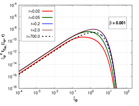
Figure 1: Non-thermal momentum distribution function $f_{Z_{\rm BL}}$ plotted as a function of the dimensionless variable $\xi_{p}$ for $\beta=1$ (left) and $\beta=10^{-3}$ (right). The curves are shown for different values of $r=\frac{M_{sc}}{T}$.

With this, we now proceed to find the non-equilibrium distribution function for our dark matter particle $\psi_{1}$ using Eq. (26). It is shown in Fig. 2 (left) for $\beta=1$. Similar to the $Z_{\rm BL}$ case, here also with the decrease of temperature more and more $\psi_{1}$ particles are produced from the decays massive bosons such as $h_{1}$, $h_{2}$ and $Z_{\rm BL}$. Hence the area under the curves increases as we go from $r=0.02$ to $r=1000$. With further increase in $r$ we expect that the rate of production of $\psi_{1}$ should decrease and consequently the (comoving) number density will cease to change, since for this high value of $r$ (low temperature) the number densities of all the decaying bosons have become extremely dilute and also $\psi_{1}$ itself is stable. This can be verified, if we compare the curves corresponding to $r=10^{3}$ and $r=10^{4}$. Similar features are also observed for $\beta=10^{-3}$ case which has been shown in Fig.  2 (right).

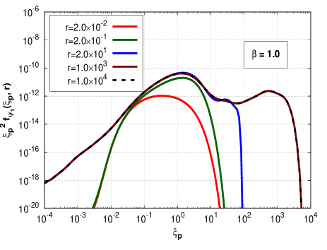
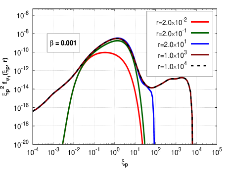
Figure 2: Non-thermal momentum distribution function $f_{\psi_{1}}$ plotted as a function of the dimensionless variable $\xi_{p}$ for $\beta=1$ (left) and $\beta=10^{-3}$ (right). The curves are shown for different values of $r=\frac{M_{sc}}{T}$.

All of the features that we have discussed so far with respect to the momentum distribution functions are reflected clearly if we plot the variation of the comoving number density of $Z_{\rm BL}$ and $\psi_{1}$ with respect to $r$. The comoving number density $Y$ is easily calculable by using Eqs. ((32) and (33)), once the momentum distribution function of the corresponding species is known . We plot our numerical results in both panels of Fig. 3.

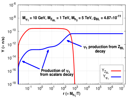
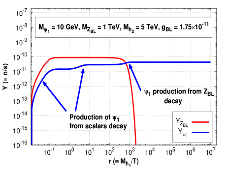
Figure 3: Variation of comoving number density of $Z_{\rm BL}$ and $\psi_{1}$ with respect to $r$. Left: $\beta=1$ and Right: $\beta=10^{-3}$.

For the $\beta=1$ case, the scalars $h_{1}$ and $h_{2}$ contribute minimally to the comoving number density of $\psi_{1}$. The bulk of the contribution comes from $Z_{\rm BL}$. In the left panel of Fig. 3, we find that the comoving number density of $Z_{\rm BL}$ first rises with $r$. Initially, there is also a similar rise in the number density of $\psi_{1}$ as well. However, the rate of increment of $Y_{\psi_{1}}$ is small compared to $Y_{Z_{\rm BL}}$ for $r\leq 0.1$ since in this regime, the main production channel of $\psi_{1}$ is the decay from BSM scalar $h_{2}$, which is presently contributing very little to $Y_{\psi}$. Then as $r$ increases, the number density of $Z_{\rm BL}$ flattens out due to the competing decay and production terms while $Y_{\psi_{1}}$ rises slightly due to its production from the decay of SM-like Higgs boson $h_{1}$. With the further increase of $r$, the $Z_{\rm BL}$ number density falls off as the decay modes of $Z_{\rm BL}$ become dominant over its production process (i.e. production from the Boltzmann suppressed $h_{2}$). Consequently, there is a sharp rise in $Y_{\psi}$ as more and more $\psi_{1}$ starts producing dominantly from $Z_{\rm BL}$ decay. Finally, for $r>10^{3}$ there is practically no $Z_{\rm BL}$ is left for decay to $\psi_{1}$, and hence in absence of any sources $Y_{\psi_{1}}$ freezes-in to a constant value. For the other case i.e. when $\beta=10^{-3}$, the situation is exactly same as with $\beta=1$ except in this case all the production modes of $\psi_{1}$ including those from the decays of $h_{1}$ and $h_{2}$ contribute equally to $Y_{\psi_{1}}$. Therefore for $r\leq 10^{2}$, $Y_{\psi_{1}}$ increases significantly since in this regime $\psi_{1}$ is mainly produced from scalars decay. Moreover unlike $Z_{\rm BL}$, as the $h_{1}$ and $h_{2}$ are in thermal equilibrium, in both panels, bulk of their contribution to the number density of $\psi_{1}$ occurs when the temperatures of the Universe are around $T\sim M_{h_{1}}$ ($r\sim 1.0$) and $T\sim M_{h_{2}}$ ($r\sim 0.03$) respectively.

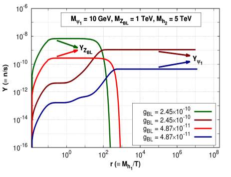
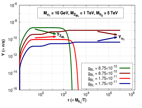
Figure 4: Variation of comoving number density of $Z_{\rm BL}$ and $\psi_{1}$ with $r$ corresponding to different values of $g_{\rm BL}$. Left: $\beta=1$ and Right: $\beta=10^{-3}$.

Let us now try to understand how the comoving number density varies with different model parameters.  Parameters have varied one at a time, while keeping the others fixed at their benchmark values. In Fig. 4, we plot the variation of $Y$ with varying $g_{\rm BL}$. Increasing $g_{\rm BL}$ will result in an increase in the collision term corresponding to $h_{2}\rightarrow Z_{\rm BL}Z_{\rm BL}$ (since $g_{h_{2}Z_{\rm BL}Z_{\rm BL}}$ increases, see Appendix A.1) and hence an enhanced initial production of $Z_{\rm BL}$. Also, increasing $g_{\rm BL}$ will enlarge the total decay width of $Z_{\rm BL}$ (see Appendix A.2 for the expression of $Z_{\rm BL}\rightarrow\,all$), and consequently we expect that the produced $Z_{\rm BL}$ will start to deplete earlier in the case where $g_{\rm BL}$ is higher. The curves corresponding to $Y_{\psi_{1}}$ follow the rise of $Z_{\rm BL}$ and in the case where $g_{\rm BL}$ is higher, more $\psi_{1}$ is produced in the final state (since there is a corresponding increment in the production of $Z_{\rm BL}$). As $Z_{\rm BL}$ depletes off, $\psi_{1}$ freezes in to a particular value of $Y_{\psi_{1}}$ as expected. In the right panel of Fig. 4, the initial sharp rise of $Y_{\psi_{1}}$ for $r\leq 10$ is due to the significant production of DM from the decaying scalars $h_{2}$ and $h_{1}$ respectively.

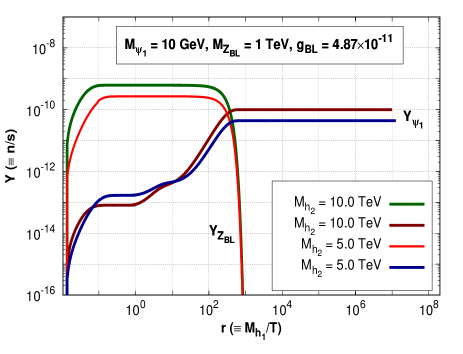
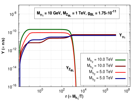
Figure 5: Variation of comoving number density of $Z_{\rm BL}$ and $\psi_{1}$ with $r$ corresponding to different values of $M_{h_{2}}$. Left: $\beta=1$ and Right: $\beta=10^{-3}$.

In Fig. 5, we have plotted the variations in $Y$ by changing $M_{h_{2}}$. Increasing $M_{h_{2}}$ will again increase $\mathcal{C}^{h_{2}\rightarrow Z_{\rm BL}\,Z_{\rm BL}}$ like the previous case. But unlike before, $Y_{Z_{\rm BL}}$ curves corresponding to the two $M_{h_{2}}$ values start falling around the same epoch. This is because, changing the mass of $h_{2}$ has no bearing upon the total decay width of $Z_{\rm BL}\rightarrow\,all$, while the latter process is responsible for the fall off. Since more $Z_{\rm BL}$ is produced initially when $M_{h_{2}}$ is increased, the yield of $\psi_{1}$ in this case is also higher, as is evident from the figure. A qualitative difference between the right and left panel of Fig. 5 is that, the final abundances of $\psi_{1}$ in $\beta=1$ case are quite different from each other for different values of $M_{h_{2}}$, while in $\beta=10^{-3}$ case, we see that they are almost identical. This is because, in the $\beta=1$ case, the contribution of the scalars are sub-dominant compared to $Z_{\rm BL}$, while abundance of the latter and consequently that of $\psi_{1}$ increases with increasing $M_{h_{2}}$. Hence the amount of splitting in the two $Y_{\psi_{1}}$ curves (left panel) is almost same as the difference observed in the corresponding $Y_{Z_{\rm BL}}$ curves. But in the $\beta=10^{-3}$ scenario, things are a little different. Here, both the scalars as well as $Z_{\rm BL}$ contribute substantially to the final abundance of $\psi_{1}$. The contribution to the final abundance from the decays of the two scalars compensates to reduce the splitting amongst the $Y_{\psi_{1}}$ curves arising from the increment of $Y_{Z_{\rm BL}}$.

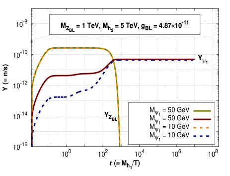
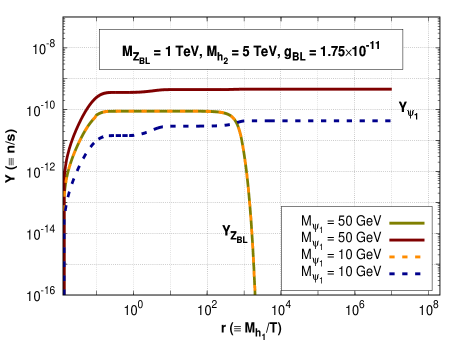
Figure 6: Variation of comoving number density of $Z_{\rm BL}$ and $\psi_{1}$ with $r$ corresponding to different values of $M_{\psi_{1}}$. Left: $\beta=1$ and Right: $\beta=10^{-3}$.

In Fig. 6, the variation of $Y_{Z_{\rm BL}}$ and $Y_{\psi_{1}}$ have been studied by changing the mass of dark matter itself i.e. $M_{\psi_{1}}$. Now in the present scenario with $M_{Z_{\rm BL}}\gg M_{\psi_{1}}$, any change in the mass of dark matter will in no way affect $Y_{Z_{\rm BL}}$, since $M_{\psi_{1}}$ neither affects the $Z_{\rm BL}$ total decay width nor does it change $h_{2}\rightarrow Z_{\rm BL}Z_{\rm BL}$ collision term. But the production of $\psi_{1}$ from the scalars decay is however affected. It is clear from the expression of the scalar–dark matter couplings given in Appendix A.1, that with increase in $M_{\psi_{1}}$, the value of the coupling increases and there by yielding more $\psi_{1}$. This observation is corroborated if we look at the blue dashed line (corresponding to $M_{\psi_{1}}=10\rm\,GeV$) and the solid grey line (corresponding to $M_{\psi_{1}}=50\rm\,GeV$) in the left panel of Fig.  6. For more massive dark matter, the yield of $\psi_{1}$ is higher from the scalars decay. But there is no effect on the production of $\psi_{1}$ from $Z_{\rm BL}$ decay, which is expected, since the couplings between $Z_{\rm BL}$ and $\psi_{1}$ do not depend on the mass of the latter and also here $M_{Z_{\rm BL}}\gg M_{\psi_{1}}$ . Let us now contrast this case with the right panel of Fig. 6. Here again as before the contribution of the scalars become important. As already mentioned, the benchmark for $\beta=10^{-3}$ scenario is chosen in such a way, so that $h_{1}$, $h_{2}$ and $Z_{\rm BL}$ contribute equally in the final relic abundance. Increase in scalar–dark matter couplings (due to an increase in $M_{\psi_{1}}$), hence makes the contribution from the scalars decay, larger than that from the $Z_{\rm BL}$.

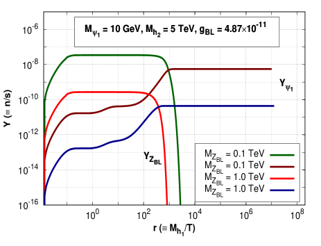
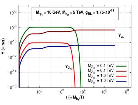
Figure 7: Variation of comoving number density of $Z_{\rm BL}$ and $\psi_{1}$ with $r$ corresponding to different values of $M_{Z_{\rm BL}}$. Left: $\beta=1$ and Right: $\beta=10^{-3}$.

In Fig. 7, variation with respect to $M_{Z_{\rm BL}}$ is demonstrated. With an increase in $M_{Z_{\rm BL}}$, the total decay width $Z_{\rm BL}\rightarrow\,all$ increases leading to an earlier fall in the comoving number density of $Z_{\rm BL}$. Also increasing $M_{Z_{\rm BL}}$ suppresses the production of $Z_{\rm BL}$ via $h_{2}$ decay. $Y_{\psi_{1}}$, on the other hand tracks the rise and fall of $Y_{Z_{\rm BL}}$ (since $Z_{\rm BL}$ is the main production channel of $\psi_{1}$ in the left panel with $\beta=1$ case). For $\beta=10^{-3}$ (right panel), $Y_{Z_{\rm BL}}$ exhibits similar features. The scalar–dark matter couplings on the other hand increases with an decrease in $M_{Z_{\rm BL}}$. This leads to higher yield of $\psi_{1}$ from scalars decay. The yield from $Z_{\rm BL}$ decay, for reasons discussed before, also increases due to a decrease in $M_{Z_{\rm BL}}$. All these are shown in the right panel of Fig. 7.

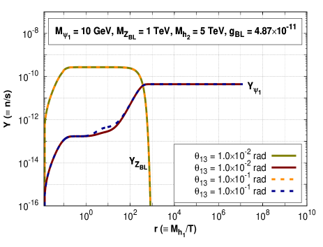
(a) Variation with different $\theta_{13}$ values for $\beta=1$

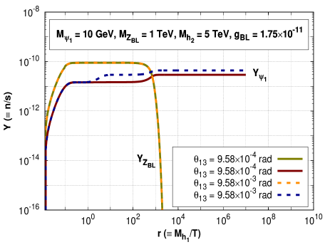
(b) Variation with different $\theta_{13}$ values for $\beta=10^{-3}$

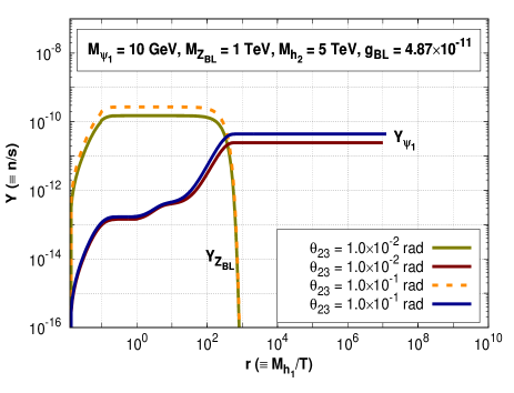
(c) Variation with different $\theta_{13}$ values for $\beta=1$

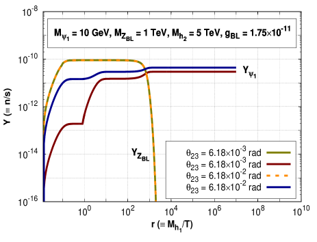
(d) Variation with different $\theta_{13}$ values for $\beta=10^{-3}$

Figure 8: Comparison of comoving number densities of $Z_{\rm BL}$ and $\psi_{1}$ with respect to mixing angles $\theta_{13}$ and $\theta_{23}$.

Let us now discuss the variation of $Y$ with respect to mixing angles. These are shown in Fig.  8 (a)–8 (d). As mentioned earlier, when $\beta=1$, the mixing angles have very little effect on the comoving number density of $Z_{\rm BL}$ and $\psi_{1}$. In Fig. 8 (a), on increasing $\theta_{13}$, we find that there is only a small increase in the production of $\psi_{1}$ from the SM Higgs ($h_{1}$) due to an increase in $g_{h_{1}\overline{\psi_{1}}\psi_{1}}$ coupling. On the other hand, $g_{h_{2}Z_{\rm BL}Z_{\rm BL}}$ is however insensitive to variations in $\theta_{13}$ and hence $Y_{Z_{\rm BL}}$ remains unchanged. The $g_{h_{2}Z_{\rm BL}Z_{\rm BL}}$ coupling, however, is sensitive to $\theta_{23}$ (because of the presence of the term like $\cos\theta_{13}\sin{\theta}_{23}$). So we find a corresponding increase in $Z_{\rm BL}$ yield on increasing $\theta_{23}$ in Fig. 8 (c). Consequently, an increase in $Y_{\psi_{1}}$ is also noted.

Variation in the yield of $Z_{\rm BL}$ and $\psi_{1}$ with these mixing angles is more pronounced in the $\beta=10^{-3}$ scenario. Increasing $\theta_{13}$ in Fig. 8 (b), we find that the production of dark matter from SM Higgs decay is enhanced while the production from $h_{2}$ is almost unaffected. This happens since the coupling $g_{h_{1}\overline{\psi_{1}}\psi_{1}}$ is more sensitive to changes in $\theta_{13}$ as is seen from its expression in the Appendix A.1. On the contrary, the coupling $g_{h_{2}\overline{\psi_{1}}\psi_{1}}$ is sensitive to $\theta_{23}$. So production of $\psi_{1}$ from $h_{2}$ is enhanced in the case where $\theta_{23}$ is increased (Fig. 8 (d)). Yield of $Z_{\rm BL}$ in this case ($\beta=10^{-3}$), however remains unaffected because the effect of the mixing angle $\theta_{13}$ on the coupling $g_{h_{2}Z_{\rm BL}Z_{\rm BL}}$ is always suppressed due to its nature of occurrence within the trigonometric functions while the low value of $\beta$ makes the $h_{2}Z_{\rm BL}Z_{\rm BL}$ coupling insensitive to the other mixing angle $\theta_{23}$.

Finally, to contrast the two scenarios, we have plotted the relic density corresponding to the two benchmarks given in Table 2. The equal contribution of the scalars as well as $Z_{\rm BL}$ to the final DM relic abundance is clearly visible in Fig. 9 for $\beta=10^{-3}$ case. In the other scenario, all most all of the contribution to the final abundance of $\psi_{1}$ comes from the decay of $Z_{\rm BL}$.

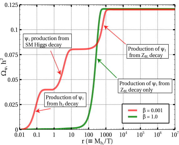
Figure 9: Variation of total relic density of $\psi_{1}$ with $r$ corresponding to $\beta=1$ and $\beta=10^{-3}$.

To get an overall idea about the allowed parameter range where our scenario satisfies DM relic density, we next perform random scans over the appropriate combination of variables. The results are shown in both panels of Fig. 10. The left panel shows our findings in $g_{\rm BL}-M_{\psi_{1}}$ plane. Now, if $g_{\rm BL}$ increases then DM production from $Z_{\rm BL}$ decay will tend to increase its contribution to the relic density. Hence to satisfy the relic density constraint, DM production

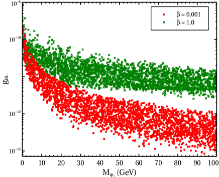
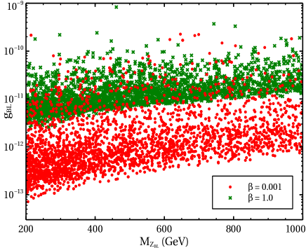
Figure 10: Points allowed by relic density constraint in $g_{\rm BL}-M_{\psi_{1}}$ (left) and $g_{\rm BL}-M_{Z_{\rm BL}}$ (right) planes. The range of variation of other relevant parameters are as follows: $200\,{\rm GeV}\leq M_{Z_{\rm BL}}\leq 1000$ GeV, $2\,M_{Z_{\rm BL}}\leq M_{h_{2}}\leq 7$ TeV, $10^{-14}\leq g_{\rm BL}\leq 10^{-9}$, $10^{-1}\,{\rm GeV}\leq M_{\psi_{1}}\leq 100$ GeV. Other independent parameters have been kept fixed to their corresponding benchmark values.

from scalar decay modes should decrease proportionately. Moreover, from the right panel of Fig. 10 where we illustrate the allowed region (which produces correct DM relic density) in $g_{\rm BL}-M_{Z_{\rm BL}}$ plane, one can see that with decreasing $g_{\rm BL}$, $M_{Z_{\rm BL}}$ also decreases. Hence, $M_{\psi_{1}}$ should decrease with increasing $g_{\rm BL}$ (see Appendix 42–44) to suppress dark matter production from the decaying heavy scalar bosons ($h_{2}$, $h_{1}$).

A major portion of this work is focussed on deriving the distribution function of the dark matter particle $\psi_{1}$. A natural question may hence arise about the need of following such a procedure. Naively, one may expect to follow the usual procedure of solving the Boltzmann equation written in terms of the comoving number density $Y$ [43, 18]. However, if the decaying mother particle is not in thermal equilibrium, then we need to solve a separate Boltzmann equation for the comoving number density of this out of equilibrium mother particle first. Because, the usual form of the Boltzmann equation in terms of $Y$ depends on the fact that the species under study is at least close to thermal equilibrium. For example, in case of DM production from a decaying species, the thermal average decay width ${\langle\Gamma\rangle}_{\rm Th}$ appearing in the Boltzmann equation, is usually given by $\dfrac{K_{1}(z)}{K_{2}(z)}\Gamma$, where $K_{1}$ and $K_{2}$ are the modified Bessel functions of order 1 and 2 respectively and $\Gamma$ is the usual decay width in the rest frame of decaying particle. However, while deriving the above expression of thermally averaged decay width one assumes that the corresponding decaying particle is either in thermal equilibrium or at least it is close to thermal equilibrium such that its obeys Maxwell-Boltzmann distribution. If this is not the case, such a thermal average is not guaranteed to give correct results and relic density should not be computed directly by solving the Boltzmann equation for $Y$. In such cases average value of the decay width itself requires the information about the non-equilibrium momentum distribution function of the decaying mother particle. Under such circumstances, ${\langle\Gamma\rangle}_{\rm Th}$ should be replaced by non-thermal average, ${\langle\Gamma\rangle}_{\rm NTh}=m\,\Gamma\,\dfrac{\int\,\frac{\,f_{\rm non-eq}(p)}{\sqrt{p^{2}+m^{2}}}\,\,d^{3}p}{\int\,f_{\rm non-eq}(p)\,d^{3}p}$ where m is the mass of the decaying species and $f_{\rm non-eq}(p)$ is its distribution function. So we should first solve the distribution function of the mother particle (here $Z_{\rm BL}$), then use it to calculate the distribution function of the dark matter directly. Once this is known, we can calculate other quantities of interest as we have discussed elaborately earlier. Thus, finally we make a comparative study (for both the benchmark points $\beta=1$ and $\beta=0.001$) of the differences in the results obtained from the exact calculation and that obtained by assuming the system to be close to an equilibrium one. The findings are plotted in both the panels of Fig. 11 where left panel is for $\beta=1$ case while the right one corresponds to $\beta=0.001$. In both plots, we find considerable differences in the final abundance of $\psi_{1}$ computed using ${\langle\Gamma\rangle}_{\rm NTh}$ (solid lines) and ${\langle\Gamma\rangle}_{\rm Th}$ (dashed lines). We also find that the difference in $Y_{\psi_{1}}$ depends on the contribution of $Z_{\rm BL}$ to comoving number density of $\psi_{1}$. For $\beta=1$ case, almost all the DM is produced from the decay of $Z_{\rm BL}$ and hence in this case, $Y_{\psi_{1}}$ obtained from exact calculation is 7.98 times lower than that obtained from the approximate one. For the other scenario, with $\beta=0.001$, contribution of $Z_{\rm BL}$ is only 33%. So now, the final value of $Y_{\psi_{1}}$ from the exact calculation using distribution functions is 3.32 times smaller than the value of $Y_{\psi_{1}}$ obtained using the approximate method.

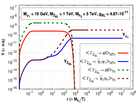
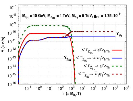
Figure 11: Comparison between the $Y_{Z_{\rm BL}}$ and $Y_{\psi_{1}}$ obtained from the exact calculation using momentum distribution approach with that of the approximate method using the ${\langle\Gamma\rangle}_{\rm Th}$ for $\beta=1$ (left panel) and $\beta=0.001$ (right panel).

5 Constraints

In this section, we will discuss about the relevant constraints on the model parameters arising from theoretical as well as experiment and observational results. To start with, we should first satisfy the nontrivial theoretical constraints arising from the vacuum stability criterion. The conditions we need to satisfy are listed in Eqs. ((3)–(4)) (copositivity conditions [44]) For a general $3\times 3$ scalar mixing matrix it is difficult to write closed form analytical expressions of the different $\lambda$’s (Eq. (1)) in terms of our chosen set of independent parameters. We have however checked numerically that for our benchmark points the conditions are indeed satisfied.

Among the experimental constraints let us first discuss the implication of the constraint related to the invisible decay width of SM $Z$ boson. As given in [45],

$$\dfrac{\Gamma(\rm Z\rightarrow invisible)}{\Gamma(\rm Z\rightarrow\nu\bar{\nu})} = 2.990\pm 0.007.$$ (35)

In our chosen model, in absence of kinetic mixing terms between the Standard Model $Z$ boson and the extra gauge boson $Z_{\rm BL}$, the former do not decay to any BSM particles. Hence Eq. (35) is trivially satisfied.

The Standard Model Higgs boson ($h_{1}$) in the representative benchmarks is lighter than the other two scalars ($h_{2}$ and $h_{3}$) as well as $Z_{\rm BL}$. As already discussed, the fermion $\psi_{2}$ and pseudo scalar $A$ are assumed to be very heavy for simplicity. Hence only allowed invisible decay mode of $h_{1}$ is to $h_{1}\rightarrow\bar{\psi_{1}}\,\psi_{1}$. But this channel is highly suppressed because of the very small value of the extra gauge coupling $g_{\rm BL}$ required to satisfy the non-thermality condition. Thus this decay width evades the bound from LHC on the invisible decay of SM Higgs boson [42].

The scattering cross section $\psi_{1}$ with the Standard Model particles is also very weak in this non-thermal regime hence the spin independent DM nucleon coherent scattering cross sections lie much below the present day direct detection bounds [6].

From cosmological point of view, the most important constraints arise from the structure formation and somewhat related to it, the bounds from dark radiation. The presence of highly relativistic particles around the Big Bang Nucleosynthesis (BBN) epoch can upset the observed structures of the galaxies. Dark matter particles if at all produced around that epoch then it has to be non-relativistic and hence should not alter the onset of BBN. Dark matter momentum distribution functions $f_{\psi_{1}}(\xi_{p},r)$ can provide us with the vital information on whether the particle is Hot or Cold. A suitable quantity to calculate in this regard is the free-streaming horizon length denoted commonly by $\lambda_{\rm fs}$ [46]. It is defined by:

$$\lambda_{\rm fs}\equiv\int_{T_{\rm production}}^{T_{\rm now}}\dfrac{\langle{\rm v}(T)\rangle}{a(T)}\dfrac{dt}{dT}\,dT\,,$$ (36)

where $T_{\rm production}$ is the temperature when almost all of the dark matter particles have been produced and the DM comoving number density already has frozen in. $T_{\rm Now}$ is the present temperature of the Universe. $\langle{\rm v}(T)\rangle$ is the average velocity of the dark matter particle and is calculable once its distribution function is known. The term $\dfrac{dt}{dT}$ can be found from the time-temperature relationship and in the radiation dominated era $\dfrac{dt}{dT}=-\left(1+\dfrac{1}{4}\dfrac{d\,\ln g_{\rho}(T)}{d\ln T}\right)\dfrac{1}{H\,T}$, where $H(T)$ is the Hubble parameter while $g_{\rho}(T)$ is the number of degrees of freedom related to the energy density of the Universe. At this point we transform the variable $T$ to our usual dimensionless variable $r=\dfrac{M_{sc}}{T}$. With this Eq. (36) becomes:

$$\lambda_{\rm fs}=\int_{r_{\rm production}}^{r_{\rm now}}\dfrac{\langle{\rm v}(r)\rangle}{a(r)}\dfrac{\widetilde{g}_{\rho}(r)}{H(r)}\dfrac{dr}{r}\,,$$ (37)

where $\widetilde{g}_{\rho}(r)=\left(1-\dfrac{1}{4}\dfrac{d\,\ln g_{\rho}(r)}{d\ln r}\right)$ and $r_{\rm production\,(now)}\equiv\dfrac{M_{sc}}{T_{\rm production\,(now)}}$. The average velocity $\langle{\rm v}(r)\rangle$ is defined as:

$$\langle{\rm v}(r)\rangle=\mathcal{B}(r)\dfrac{\bigint_{0}^{\infty}d\xi\frac{\xi^{3}f_{\psi_{1}}(\xi,r)}{\sqrt{\mathcal{B}(r)^{2}\xi^{2}+r^{2}\frac{M_{\psi_{1}}^{2}}{M_{sc}^{2}}}}}{\bigint_{0}^{\infty}d\xi\,\xi^{2}f_{\psi_{1}}(\xi,r)}\,.$$ (38)

The scale factor $a(r)$ is obtained by using the conservation of total entropy of the Universe in a comoving volume. It is given by:

$$a(r)=\left(\dfrac{43}{11\,g_{s}(r)}\right)^{1/3}\dfrac{r}{r_{\rm now}}\,.$$ (39)

The Hubble parameter in terms of $r$ is written as:

$$H(r)=\dfrac{M_{sc}^{2}}{M_{0}(r)\,r^{2}}\,,$$ (40)

with $M_{0}(r)=\left(\dfrac{45M_{Pl}^{2}}{4\pi^{3}g_{\rho}(r)}\right)^{1/2}$ Using all these in Eq. (37) we calculated the free streaming horizon length. According to Ref. [47], if $\lambda_{fs}<0.01$ Mpc, then we can attribute the dark matter as “Cold”. In our case we have found out that $\lambda_{\rm fs}\ll 0.01$ Mpc for all the benchmark points, and hence respects the structure formation constraints.

Another cosmological quantity of interest that measures the amount of relativistic particles that can be injected without disrupting the precise experimental observations around BBN and CMB is the effective number of neutrinos, denoted by $N_{eff}$. Its standard value is given by 3.046 [48]. This number will change if the highly relativistic particles are introduced at around the time of BBN and CMB. Stringent bounds on the amount of extra relativistic degree of freedom that can be added is given by $\Delta N_{eff}$. The present experimental constraints on this quantity are $\Delta N_{eff}(T_{\rm BBN})<0.85$ [49] and $\Delta N_{eff}(T_{CMB})<0.32$ [2]. This quantity can be also calculated using the knowledge of momentum distribution function of $\psi_{1}$ following [37]. The expression of $\Delta N_{eff}$ is given by :

$$\Delta N_{eff}(r)=\frac{60}{7\pi^{4}}\left(\dfrac{r_{\nu}}{r}\right)^{4}\dfrac{M_{\psi_{1}}\,r}{M_{sc}}\mathcal{B}(r)^{3}\int_{0}^{\infty}d\xi_{p}\,\xi_{p}^{2}\left(\sqrt{1+\left(\dfrac{\mathcal{B}(r)\,\xi_{p}\,M_{sc}}{M_{\psi_{1}}\,r}\right)^{2}}-1\right)\,f_{\psi_{1}}(\xi_{p},r)\,.$$ (41)

The factor $\left(\dfrac{r_{\nu}}{r}\right)^{4}=\left(\dfrac{T}{T_{\nu}}\right)^{4}$ is neglected for $T\mathrel{\mathchoice{\vbox{\offinterlineskip\halign{\hfil$\displaystyle#$\hfil\cr>\cr\sim\cr}}}{\vbox{\offinterlineskip\halign{\hfil$\textstyle#$\hfil\cr>\cr\sim\cr}}}{\vbox{\offinterlineskip\halign{\hfil$\scriptstyle#$\hfil\cr>\cr\sim\cr}}}{\vbox{\offinterlineskip\halign{\hfil$\scriptscriptstyle#$\hfil\cr>\cr\sim\cr}}}}1$ MeV since the neutrinos had the same temperature with the background photon bath during that epoch. For our benchmarks, the calculated value of this $\Delta N_{eff}$ (at both the epochs of BBN and CMB) lies well below the existing upper bounds. It is expected that our scenario will not disturb the evolution of Universe during BBN and CMB. This is because in our chosen benchmarks, the mass of dark matter is $\mathcal{O}$(Gev) and most of it are produced at around a temperature of $\mathcal{O}$(100 MeV). Hence by the time the Universe is cooled to lower temperatures most of these particles will become non-relativistic and hence wont affect either structure formation or CMB.

6 Conclusion

In this work, we have calculated the momentum distribution function of a non-thermal fermionic dark matter. Calculation of momentum distribution function is a general feature of any non-thermal dark matter scenario if the dark matter particle under study originates from a parent particle that itself is outside the thermal soup. On the other hand, the momentum distribution function of DM is a key quantity for the computations of all the relevant thermodynamic quantities. We have demonstrated its use in the calculations of cosmological constraints, which, though weak in our case, can become important for other different combination of model parameters. The model chosen here is also well motivated, since it is anomaly free and also explains the genesis of neutrino mass, besides accommodating a non-thermal fermionic dark matter candidate as well. For the two chosen benchmark scenarios there are noticeable structural differences in the plots. In one scenario (with $\beta=1$), the dominant production of dark matter is seen to be pronounced from $Z_{\rm BL}$ decay and hence the final abundances is not much sensitive to the scalars mixing angles. In the other scenario (with $\beta(\ll 1)=10^{-3}$), however all decay modes can contribute substantially, resulting in a characteristic multi-plateau feature in the variation of comoving number density ($Y_{\psi_{1}}$) with $r$. Finally, we have also checked that our non-thermal dark matter scenario does not violate any experimental or theoretical constraints.

7 Acknowledgement

Authors would like to acknowledge Department of Atomic Energy (DAE), Govt. of INDIA for financial assistance.

Appendix A Appendix

A.1 Relevant Vertex factors

We denote the vertex factor by $g_{abc}$ for a vertex containing fields $a,\,b,\,c$. Vertex factors for the interactions of $\psi_{1}$ with CP-even scalars are given below

$$g_{h_{1}\overline{\psi_{1}}\psi_{1}} = 2\sqrt{2}\,\dfrac{g_{\rm BL}\,\sqrt{1+4\,\beta^{2}}}{\beta\,M_{Z_{\rm BL}}}\left(\beta\,\sin\theta_{12}\cos\theta_{13}\cos^{2}\theta_{\rm L}M_{\psi_{1}}+\sin\theta_{13}\sin^{2}\theta_{\rm L}M_{\psi_{1}}\right)$$ (42)

$$g_{h_{2}\overline{\psi_{1}}\psi_{1}} = 2\sqrt{2}\,\dfrac{g_{\rm BL}\,\sqrt{1+4\,\beta^{2}}}{\beta\,M_{Z_{\rm BL}}}\left(\beta\,\left(\cos\theta_{12}\cos\theta_{23}-\sin\theta_{12}\sin\theta_{23}\sin\theta_{13}\right)\cos^{2}\theta_{\rm L}M_{\psi_{1}}\right.$$ (43)

$$\left.+\sin\theta_{23}\cos\theta_{13}\sin^{2}\theta_{\rm L}M_{\psi_{1}}\right)$$

$$g_{h_{3}\overline{\psi_{1}}\psi_{1}} = 2\sqrt{2}\,\dfrac{g_{\rm BL}\,\sqrt{1+4\,\beta^{2}}}{\beta\,M_{Z_{\rm BL}}}\left(-\beta\,\left(\cos\theta_{12}\sin\theta_{23}+\sin\theta_{12}\cos\theta_{23}\sin\theta_{13}\right)\cos^{2}\theta_{\rm L}M_{\psi_{1}}\right.$$ (44)

$$\left.+\cos\theta_{23}\cos\theta_{13}\sin^{2}\theta_{\rm L}M_{\psi_{1}}\right)$$

Vertex factors for the interactions between CP-even scalars and ${\rm B-L}$ gauge boson ($Z_{\rm BL}$):

$$g_{h_{1}Z_{\rm BL}Z_{\rm BL}} = 2\,\dfrac{g_{\rm BL}\,M_{Z_{\rm BL}}}{\sqrt{1+4\beta^{2}}}\left(\sin\theta_{12}\cos\theta_{13}+4\beta\sin\theta_{13}\right)$$ (45)

$$g_{h_{2}Z_{\rm BL}Z_{\rm BL}} = 2\,\dfrac{g_{\rm BL}\,M_{Z_{\rm BL}}}{\sqrt{1+4\beta^{2}}}\left(\cos\theta_{12}\cos\theta_{23}-\sin\theta_{12}\sin\theta_{23}\sin\theta_{13}+4\beta\cos\theta_{13}\sin\theta_{23}\right)$$ (46)

$$g_{h_{3}Z_{\rm BL}Z_{\rm BL}} = 2\,\dfrac{g_{\rm BL}\,M_{Z_{\rm BL}}}{\sqrt{1+4\beta^{2}}}\left(-\left(\cos\theta_{12}\sin\theta_{23}+\sin\theta_{12}\cos\theta_{23}\sin\theta_{13}\right)+4\beta\cos\theta_{13}\cos\theta_{23}\right)$$ (47)

The interaction vertex of the dark matter $\psi_{1}$ with the new gauge boson can be written as: $\frac{g_{\rm BL}}{6}\,\overline{\psi}_{1}\gamma^{\mu}\left(a-b\,\gamma_{5}\right)\psi_{1}$, where $a=(1-3\sin^{2}\theta_{\rm L})$ and $b=-3\,(1+\sin^{2}\theta_{\rm L})$.

The Yukawa couplings of the fermions i.e. the ${y_{\xi}}_{i}$’s and ${y_{\eta}}_{i}$’s are also listed below for completeness.

$${y_{\xi}}_{1} = \sqrt{2}\,\dfrac{g_{\rm BL}\sqrt{1+4\beta^{2}}}{\beta\,M_{Z_{\rm BL}}}\left(\cos\theta_{\rm L}\cos\theta_{\rm R}\,M_{\psi_{2}}+\sin\theta_{\rm L}\sin\theta_{\rm R}\,M_{\psi_{1}}\right),$$ (48)

$${y_{\xi}}_{2} = \sqrt{2}\,\dfrac{g_{\rm BL}\sqrt{1+4\beta^{2}}}{\beta\,M_{Z_{\rm BL}}}\left(-\cos\theta_{\rm L}\sin\theta_{\rm R}\,M_{\psi_{2}}+\sin\theta_{\rm L}\cos\theta_{\rm R}\,M_{\psi_{1}}\right),$$ (49)

$${y_{\eta}}_{1} = \sqrt{2}\,\dfrac{g_{\rm BL}\sqrt{1+4\beta^{2}}}{M_{Z_{\rm BL}}}\left(-\sin\theta_{\rm L}\cos\theta_{\rm R}\,M_{\psi_{2}}+\cos\theta_{\rm L}\sin\theta_{\rm R}\,M_{\psi_{1}}\right),$$ (50)

$${y_{\eta}}_{2} = \sqrt{2}\,\dfrac{g_{\rm BL}\sqrt{1+4\beta^{2}}}{M_{Z_{\rm BL}}}\left(\sin\theta_{\rm L}\sin\theta_{\rm R}\,M_{\psi_{2}}+\cos\theta_{\rm L}\cos\theta_{\rm R}\,M_{\psi_{1}}\right).$$ (51)

A.2 Relevant Decay Widths

The only relevant decay widths that we need during the computation of dark matter momentum distribution functions are those corresponding to the decay of the extra gauge boson $Z_{\rm BL}$ to fermions.

$$\Gamma_{Z_{\rm BL}\rightarrow f\bar{f}} = \dfrac{M_{Z_{\rm BL}}}{16\pi}\dfrac{4}{3}\left(a_{f}^{2}+b_{f}^{2}\right)\Bigg{(}1+\dfrac{2\left(a_{f}^{2}-2b_{f}^{2}\right)}{\left(a_{f}^{2}+b_{f}^{2}\right)}\dfrac{M_{f}^{2}}{M_{Z_{\rm BL}}^{2}}\Bigg{)}\sqrt{1-\dfrac{4M_{f}^{2}}{M_{Z_{\rm BL}}^{2}}}\,.$$ (52)

If $f$ is a Standard Model fermion then $b_{f}=0$ and $a_{f}=g_{\rm BL}\,Q_{\rm BL}(f)$, where $Q_{\rm BL}(f)$ is the $B-L$ charge corresponding to the fermion $f$ (see Table 1). If, on the other hand $f$ is a beyond Standard Model particle (say, $f=\psi_{1}$), we have $a_{\psi_{1}}=\frac{g_{\rm BL}}{6}\left(1-3\sin^{2}\theta_{\rm L}\right)$ and $b_{\psi_{1}}=\frac{g_{\rm BL}}{2}\left(1+\sin^{2}\theta_{\rm L}\right)$. Hence the total decay width (assuming other BSM particles such as $\psi_{2}$, $A$ and $h_{3}$ are heavier than $Z_{\rm BL}$) is given as the sum of the individual decay widths to all these individual SM and BSM channels i.e.

$$\Gamma_{Z_{\rm BL}\rightarrow all}=\left(\sum\limits_{\rm SM\,fermions}\Gamma_{Z_{\rm BL}\rightarrow f\bar{f}}\right)+\Gamma_{Z_{\rm BL}\rightarrow\psi_{1}\overline{\psi_{1}}}\,.$$ (53)

Note, that this expression of decay width is valid only in the rest frame of the decaying particle (here $Z_{\rm BL}$). In a reference frame where $Z_{\rm BL}$ is not at rest but moving with an energy $E_{Z_{\rm BL}}$, the total decay width is given by:

$$\Gamma_{Z_{\rm BL}\rightarrow all}^{\prime}=\Gamma_{Z_{\rm BL}\rightarrow all}\,\frac{M_{Z_{\rm BL}}}{E_{Z_{\rm BL}}}$$ (54)

A.3 Collision terms

The first step while solving the Boltzmann equation is to derive the collision terms ($\mathcal{C}[f]$). The generic form of the collision term in case of $1\rightarrow 2$ decay process (say, $\chi\rightarrow a\,b$) is given by [50, 5]:

$$\mathcal{C}[f_{\chi}(p)] = \dfrac{1}{2\,E_{p}}\bigintsss\dfrac{g_{a}\,d^{3}p^{\prime}}{(2\pi)^{3}\,2E_{p^{\prime}}}\dfrac{g_{b}\,d^{3}q^{\prime}}{(2\pi)^{3}\,2E_{q^{\prime}}}(2\pi)^{4}\,\delta^{4}(\tilde{p}-\tilde{p}^{\prime}-\tilde{q}^{\prime})\times\overline{\,\lvert\mathcal{M}\rvert^{2}}$$ (55)

$$\leavevmode\nobreak\ \leavevmode\nobreak\ \leavevmode\nobreak\ \leavevmode\nobreak\ \leavevmode\nobreak\ \leavevmode\nobreak\ \leavevmode\nobreak\ \leavevmode\nobreak\ \leavevmode\nobreak\ \leavevmode\nobreak\ \leavevmode\nobreak\ \leavevmode\nobreak\ \leavevmode\nobreak\ \leavevmode\nobreak\ \times\,[f_{a}\,f_{b}\,\left(1\pm f_{\chi}\right)-f_{\chi}\left(1\pm f_{a}\right)\left(1\pm f_{b}\right)]\,.$$

In this expression $p,p^{\prime},q^{\prime}$ are the absolute values of three momenta of $\chi,\,a$ and $b$ respectively. The corresponding four momenta are given by $\tilde{p},\,\tilde{p}^{\prime}$ and $\tilde{q}^{\prime}$ while $E_{p},\,E_{p^{\prime}}$ and $E_{q^{\prime}}$ are the energies of $\chi,\,a$ and $b$ respectively. These energies are of course related to the absolute value of the corresponding three momenta by the usual relativistic dispersion relation. For e.g. $E_{p}=\sqrt{p^{2}+m_{\chi}^{2}}$ and so on. The internal degrees of freedom corresponding to the particles $a$ and $b$ are indicated by $g_{a}$ and $g_{b}$ respectively. The matrix element squared denoted by $\overline{\,\lvert\mathcal{M}\rvert^{2}}$ for the corresponding process (here, $\chi\rightarrow a\,b$) is averaged over the spins of both the initial as well as final state particles. The distribution function corresponding to the particle $x$ is denoted by $f_{x}$ and $(1\pm f_{x})$ are the Pauli blocking and the stimulated emission factors respectively. These factors can be approximated $\sim 1$ in absence of Bose condensation and Fermi degeneracy. If any of the particles $a$ or $b$ is in thermal equilibrium then the corresponding $f$ can be approximated by the Maxwell-Boltzmann distribution function i.e. $f\sim e^{-\frac{E}{T}}$, where $E$ is the energy of the particle and $T$ is the temperature of the Universe.

A.3.1 $\boldsymbol{\mathcal{C}^{Z_{\rm BL}\rightarrow all}}$

As a concrete example let us try to calculate ${\mathcal{C}^{Z_{\rm BL}\rightarrow all}}$ (the second collision term in Eq. (25)). Let us first calculate the collision term for a specific channel, say $\mathcal{C}^{Z_{\rm BL}\rightarrow f\bar{f}}$, where $f$ is any fermion. In Eq. (25), we are interested in solving the non-equilibrium distribution function for $Z_{\rm BL}$. Hence this collision term denotes the depletion of the particle under study. If we neglect the back reactions i.e. the inverse decay processes (which is a legitimate approximation for a particle in non-thermal regime [36, 37]) and approximate the Pauli blocking factors and stimulated emission terms to be $\sim$ 1, then from Eq. (55) we have:

$$\mathcal{C}^{Z_{\rm BL}\rightarrow f\bar{f}}[f_{Z_{\rm BL}}(p)] = \dfrac{1}{2\,E_{p}}\bigintsss\dfrac{g_{f}\,d^{3}p^{\prime}}{(2\pi)^{3}\,2E_{p^{\prime}}}\dfrac{g_{f}\,d^{3}q^{\prime}}{(2\pi)^{3}\,2E_{q^{\prime}}}(2\pi)^{4}\,\delta^{4}(\tilde{p}-\tilde{p}^{\prime}-\tilde{q}^{\prime})\times\overline{\,\lvert\mathcal{M}\rvert^{2}}$$

$$\leavevmode\nobreak\ \leavevmode\nobreak\ \leavevmode\nobreak\ \leavevmode\nobreak\ \leavevmode\nobreak\ \leavevmode\nobreak\ \leavevmode\nobreak\ \leavevmode\nobreak\ \leavevmode\nobreak\ \leavevmode\nobreak\ \leavevmode\nobreak\ \leavevmode\nobreak\ \leavevmode\nobreak\ \leavevmode\nobreak\ \times[-f_{Z_{\rm BL}}(p)]\,,$$

$$= -f_{Z_{\rm BL}}(p)\times\dfrac{1}{2\,E_{p}}\bigintsss\dfrac{g_{f}\,d^{3}p^{\prime}}{(2\pi)^{3}\,2E_{p^{\prime}}}\dfrac{g_{f}\,d^{3}q^{\prime}}{(2\pi)^{3}\,2E_{q^{\prime}}}(2\pi)^{4}\,\delta^{4}(\tilde{p}-\tilde{p}^{\prime}-\tilde{q}^{\prime})\times\overline{\,\lvert\mathcal{M}\rvert^{2}}\,.$$

But we know that the decay width (in an arbitrary frame) for the process $Z_{\rm BL}\rightarrow f\bar{f}$ is given by the expression:

$$\Gamma_{Z_{\rm BL}\rightarrow f\bar{f}}^{\prime} = \dfrac{1}{2\,E_{p}}\bigintsss\dfrac{g_{f}\,d^{3}p^{\prime}}{(2\pi)^{3}\,2E_{p^{\prime}}}\dfrac{g_{f}\,d^{3}q^{\prime}}{(2\pi)^{3}\,2E_{q^{\prime}}}(2\pi)^{4}\,\delta^{4}(\tilde{p}-\tilde{p}^{\prime}-\tilde{q}^{\prime})\times\overline{\,\lvert\mathcal{M}\rvert^{2}}\Bigg{\lvert}_{Z_{\rm BL}\rightarrow f\bar{f}}\,,$$ (57)

where, as discussed before, $p,\,p^{\prime}$ and $q^{\prime}$ are the three momenta corresponding to $Z_{\rm BL},\,f$ and $\bar{f}$ respectively. Now using Eq. (57) in Eq. (55) and making the change of variables $\xi_{p}\equiv\dfrac{1}{\mathcal{B}(r)}\,\dfrac{p}{T}$ and $r_{Z_{\rm BL}}\equiv\dfrac{M_{Z_{\rm BL}}}{T}$, we get

$$\mathcal{C}^{Z_{\rm BL}\rightarrow f\bar{f}}[f_{Z_{\rm BL}}(\xi_{p})] = -f_{Z_{\rm BL}}(\xi_{p})\times\Gamma_{Z_{\rm BL}\rightarrow f\bar{f}}\times\dfrac{M_{Z_{\rm BL}}}{E_{Z_{\rm BL}}}\,,$$ (58)

$$= -f_{Z_{\rm BL}}(\xi_{p})\times\Gamma_{Z_{\rm BL}\rightarrow f\bar{f}}\times\dfrac{r_{Z_{\rm BL}}}{\sqrt{\xi_{p}^{2}\,\mathcal{B}(r)^{2}+r_{Z_{\rm BL}}^{2}}}\,,$$

where we have used Eq. (54). Hence the collision term $\mathcal{C}^{Z_{\rm BL}\rightarrow all}$ is now simply given by:

$$\mathcal{C}^{Z_{\rm BL}\rightarrow all} = -f_{Z_{\rm BL}}(\xi_{p})\times\Gamma_{Z_{\rm BL}\rightarrow all}\times\dfrac{r_{Z_{\rm BL}}}{\sqrt{\xi_{p}^{2}\,\mathcal{B}(r)^{2}+r_{Z_{\rm BL}}^{2}}}\,.$$ (59)

We can easily rewrite the above equation in terms of $r\equiv\frac{M_{sc}}{T}$ by writing $r_{Z_{\rm BL}}=\frac{M_{Z_{\rm BL}}}{M_{sc}}\,r$.

The derivation of this collision term is greatly simplified by the use of the expression of the decay width (Eq. (57)). This simplification is possible because the distribution function of the particle we are interested in (i.e. $Z_{\rm BL}$) is itself the decaying particle.

However, the situation may be such that the particle whose non-equilibrium momentum distribution function we are interested in, is the daughter particle produced from the decay of another mother particle (where it is assumed that the distribution function of the latter is already known). In that case, the final expression for the collision term will not be so simple. We will illustrate such a case now with a definite example. Let us hence derive the first collision term in Eq. (25) i.e. ${\mathcal{C}^{h_{2}\rightarrow Z_{\rm BL}Z_{\rm BL}}}$.

A.3.2 $\boldsymbol{\mathcal{C}^{h_{2}\rightarrow Z_{\rm BL}Z_{\rm BL}}}$

The starting point is again Eq. (55). This is actually the first collision term in Eq. (25). Proceeding as before we now have:

$$\mathcal{C}^{h_{2}\rightarrow Z_{\rm BL}Z_{\rm BL}}[f_{Z_{\rm BL}}(p)] = 2\times\dfrac{1}{2\,E_{p}}\bigintsss\dfrac{g_{h_{2}}\,d^{3}k}{(2\pi)^{3}\,2E_{k}}\dfrac{g_{Z_{\rm BL}}\,d^{3}q^{\prime}}{(2\pi)^{3}\,2E_{q^{\prime}}}(2\pi)^{4}\,\delta^{4}(\tilde{k}-\tilde{p}-\tilde{q}^{\prime})\times\overline{\,\lvert\mathcal{M}\rvert^{2}}\bigg{\lvert}_{h_{2}\rightarrow Z_{\rm BL}Z_{\rm BL}}$$ (60)

$$\leavevmode\nobreak\ \leavevmode\nobreak\ \leavevmode\nobreak\ \leavevmode\nobreak\ \leavevmode\nobreak\ \leavevmode\nobreak\ \leavevmode\nobreak\ \leavevmode\nobreak\ \leavevmode\nobreak\ \leavevmode\nobreak\ \leavevmode\nobreak\ \leavevmode\nobreak\ \leavevmode\nobreak\ \leavevmode\nobreak\ \times\,[f_{h_{2}}\left(1\pm f_{Z_{\rm BL}}\right)\left(1\pm f_{Z_{\rm BL}}\right)-f_{Z_{\rm BL}}\,f_{Z_{\rm BL}}\,\left(1\pm f_{h_{2}}\right)]\,.$$

Here $k$ is the three momentum of the decaying particle ($h_{2}$) while $p$ and $q^{\prime}$ are the three momenta of the final state particles ($Z_{\rm BL}$). The factor of $2$ in front is due the production of two $Z_{\rm BL}$ in the final state from $h_{2}$ decay. $g_{Z_{\rm BL}}$ and $g_{h_{2}}$ are the internal degrees of freedom for the extra gauge boson and extra scalar respectively. Hence, $g_{Z_{\rm BL}}=3$ and $g_{h_{2}}=1$.

Using the usual approximations of neglecting the back reactions as well as the Pauli blocking and stimulated emission factors, we finally get:

$$\mathcal{C}^{h_{2}\rightarrow Z_{\rm BL}Z_{\rm BL}}[f_{Z_{\rm BL}}(p)] = 2\times\dfrac{1}{2\,E_{p}}\bigintsss\dfrac{g_{h_{2}}\,d^{3}k}{(2\pi)^{3}\,2E_{k}}\dfrac{g_{Z_{\rm BL}}\,d^{3}q^{\prime}}{(2\pi)^{3}\,2E_{q^{\prime}}}(2\pi)^{4}\,\delta^{4}(\tilde{k}-\tilde{p}-\tilde{q}^{\prime})\times\overline{\,\lvert\mathcal{M}\rvert^{2}}\bigg{\lvert}_{h_{2}\rightarrow Z_{\rm BL}Z_{\rm BL}}$$ (61)

$$\leavevmode\nobreak\ \leavevmode\nobreak\ \leavevmode\nobreak\ \leavevmode\nobreak\ \leavevmode\nobreak\ \leavevmode\nobreak\ \leavevmode\nobreak\ \leavevmode\nobreak\ \leavevmode\nobreak\ \leavevmode\nobreak\ \leavevmode\nobreak\ \leavevmode\nobreak\ \leavevmode\nobreak\ \leavevmode\nobreak\ \times\,[f_{h_{2}}(k)]\,.$$

The matrix element squared average for the decay process $h_{2}\rightarrow Z_{\rm BL}Z_{\rm BL}$ is given by:

$$\overline{\,\lvert\mathcal{M}\rvert^{2}}\bigg{\lvert}_{h_{2}\rightarrow Z_{\rm BL}Z_{\rm BL}} = \dfrac{g_{h_{2}Z_{\rm BL}Z_{\rm BL}}^{2}}{2\times 9}\Bigg{(}2+\dfrac{\left(E_{p}E_{q^{\prime}}-\vec{p}\,.\,\vec{q^{\prime}}\,\right)^{2}}{M_{Z_{\rm BL}}^{4}}\,\Bigg{)}\,.$$ (62)

In Eq. (61), $\delta^{(4)}(\tilde{k}-\tilde{p}-\tilde{q}^{\prime})$ can be written as $\delta^{(3)}(\vec{k}-\vec{p}-\vec{q}^{\prime})\,\delta(E_{k}-E_{p}-E_{q^{\prime}})$. We can then do the integral over $q^{\prime}$. So we should replace every occurrence of $\vec{q^{\prime}}$ with $\vec{k}-\vec{p}$. As already stated earlier that, to simplify notations we will write $\lvert\vec{k}\rvert=k$ and so on. Hence now $E_{q^{\prime}}$ has become a function of $p$ and $k$ (and of the masses of the corresponding particles which have three momenta $\vec{p}$ and $\vec{k}$ respectively), i.e. $E_{q^{\prime}}=E_{q{\prime}}\,(p,k)$. Therefore Eq. (61) becomes:

$$\mathcal{C}^{h_{2}\rightarrow Z_{\rm BL}Z_{\rm BL}}[f_{Z_{\rm BL}}(p)] = \dfrac{g_{h_{2}Z_{\rm BL}Z_{\rm BL}}^{2}}{6\,(4\pi)^{2}}\dfrac{1}{E_{p}}\bigintsss\dfrac{d^{3}k}{E_{k}\,E_{q^{\prime}}(p,k)}\,\delta\left(E_{k}-E_{p}-E_{q^{\prime}}(p,k)\right)\times$$ (63)

$$\leavevmode\nobreak\ \leavevmode\nobreak\ \leavevmode\nobreak\ \leavevmode\nobreak\ \leavevmode\nobreak\ \leavevmode\nobreak\ \leavevmode\nobreak\ \Bigg{(}2+\dfrac{\left(E_{p}E_{q^{\prime}}\,(k,p)+p^{2}-p\,k\cos\theta\right)^{2}}{M_{Z_{\rm BL}}^{4}}\,\Bigg{)}\times\,[f_{h_{2}}(k)]\,,$$

where $\theta$ is the angle between the $\vec{k}$ and $\vec{p}$. Also, we have, $E_{q^{\prime}}=\sqrt{k^{2}+p^{2}+M_{Z_{\rm BL}}^{2}-2p\,k\cos\theta}$. At this point let us transform variables to $\xi_{k}=\dfrac{1}{\mathcal{B}(r)}\,\dfrac{k}{T},\,\xi_{p}=\dfrac{1}{\mathcal{B}(r)}\,\dfrac{p}{T}$ and $\cos\theta=y$, where $\mathcal{B}(r)$ is defined by Eq. (27). Also $r_{Z_{\rm BL}}=\dfrac{M_{Z_{\rm BL}}}{T}$ and $r_{h_{2}}=\dfrac{M_{h_{2}}}{T}$. Hence,

$$E_{q^{\prime}} = T\sqrt{\xi_{k}^{2}\,\mathcal{B}(r)^{2}+\xi_{p}^{2}\,\mathcal{B}(r)^{2}+r_{Z_{\rm BL}}^{2}-2\mathcal{B}(r)^{2}\,\xi_{k}\,\xi_{p}\,y}\equiv T\,H_{1}\,(\xi_{k},\xi_{p},y).$$ (64)

From here onwards, for notational fluidity, we will suppress the explicit dependence on $r\equiv\frac{M_{sc}}{T}$. Every occurrence of $r_{Z_{\rm BL}}$ and/or $r_{h_{2}}$ should be replaced by $r_{Z_{\rm BL}}=\frac{M_{Z_{\rm BL}}}{M_{sc}}\,r$ and $r_{h_{2}}=\frac{M_{h_{2}}}{M_{sc}}\,r$. Hence it is easy to identify the functional dependence on $r$. Eq. (63) now simplifies to:

$$\mathcal{C}^{h_{2}\rightarrow Z_{\rm BL}Z_{\rm BL}}[f_{Z_{\rm BL}}(\xi_{p})]=\dfrac{g_{h_{2}Z_{\rm BL}Z_{\rm BL}}^{2}}{48\pi\,T}\dfrac{\mathcal{B}(r)^{3}}{\sqrt{\xi_{p}^{2}\,\mathcal{B}(r)^{2}+r_{Z_{\rm BL}}^{2}}}\bigintsss\dfrac{\xi_{k}^{2}\,d\xi_{k}\,dy}{\sqrt{\xi_{k}^{2}\,\mathcal{B}(r)^{2}+r_{h_{2}}^{2}}\,H_{1}(\xi_{k},\xi_{p},y)}\,\delta\left(\mathcal{F}(\xi_{k},\xi_{p},y)\right)$$

$$\times\Bigg{(}2+\dfrac{\left(\sqrt{\xi_{p}^{2}\,\mathcal{B}(r)^{2}+r_{Z_{\rm BL}}^{2}}\,H_{1}(\xi_{k},\xi_{p},y)+\xi_{p}^{2}\mathcal{B}(r)^{2}-\mathcal{B}(r)^{2}\,\xi_{p}\,\xi_{k}\,y\right)^{2}}{r_{Z_{\rm BL}}^{4}}\,\Bigg{)}\times[f_{h_{2}}(\xi_{k})]\,.$$

(65)

For convenience we have defined:

$$\mathcal{F}(\xi_{k},\xi_{p},y) \equiv \sqrt{\xi_{k}^{2}+r_{h_{2}}^{2}}-\sqrt{\xi_{p}^{2}\,\mathcal{B}(r)^{2}+r_{Z_{\rm BL}}^{2}}-H_{1}(\xi_{k},\xi_{p},y)\,.$$ (66)

Also let,

$$H_{2}(\xi_{k},\xi_{p},y) \equiv \dfrac{\left(\sqrt{\xi_{p}^{2}\,\mathcal{B}(r)^{2}+r_{Z_{\rm BL}}^{2}}\,H_{1}(\xi_{k},\xi_{p},y)+\xi_{p}^{2}\,\mathcal{B}(r)^{2}-\mathcal{B}(r)^{2}\,\xi_{p}\,\xi_{k}\,y\right)^{2}}{r_{Z_{\rm BL}}^{4}}\,.$$ (67)

The $y$ integral in Eq. (65) can easily be done. For this, we have used the well known property of $\delta$ function which is $\delta(\mathcal{F}(\xi_{k},\xi_{p},y))=\dfrac{\delta(y-y_{0})}{\lvert\mathcal{F}^{\prime}(\xi_{k},\xi_{p},y_{0})\rvert}$, $\mathcal{F}^{\prime}(\xi_{k},\xi_{p},y_{0})$ denotes differentiation of $\mathcal{F}(\xi_{k},\xi_{p},y)$ with respect to $y$ at $y=y_{0}$ where $y_{0}$ is the root of the equation $\mathcal{F}(\xi_{k},\xi_{p},y)=0$. The expression of $y_{0}$ is given by:

$$y_{0}(\xi_{k},\xi_{p}) = \dfrac{1}{2\,\mathcal{B}(r)^{2}\,\xi_{k}\,\xi_{p}}\left(2\sqrt{\xi_{k}^{2}\,\mathcal{B}(r)^{2}+r_{h_{2}}^{2}}\sqrt{\xi_{p}^{2}\,\mathcal{B}(r)^{2}+r_{Z_{\rm BL}}^{2}}-r_{h_{2}}^{2}\right)\,.$$ (68)

Using this we find that

$$\mathcal{F}^{\prime}(\xi_{k},\xi_{p}) = \dfrac{\mathcal{B}(r)^{2}\,\xi_{k}\,\xi_{p}}{\sqrt{\xi_{k}^{2}\,\mathcal{B}(r)^{2}+r_{h_{2}}^{2}}-\sqrt{\xi_{p}^{2}\,\mathcal{B}(r)^{2}+r_{Z_{\rm BL}}^{2}}}\equiv F(\xi_{k},\xi_{p})\,.$$ (69)

But since $y_{0}$ is a function of $\xi_{k}$ itself, integration over $y$ puts a limit on the $\xi_{k}$ integral as well. The limit(s) can be derived by remembering that $y_{0}$ is actually $\cos\theta_{0}$, and hence $\lvert y_{0}\rvert\leq 1$. The minimum and maximum limits on $\xi_{k}$ turn out to be:

$$\xi_{k}^{\rm min}(\xi_{p}) = \dfrac{1}{2\,\mathcal{B}(r)\,r_{Z_{\rm BL}}}\bigg{\lvert}\,\eta(\xi_{p})-\mathcal{B}(r)\dfrac{\xi_{p}\,r_{h_{2}}^{2}}{r_{Z_{\rm BL}}}\bigg{\rvert}\,,$$ (70)

$$\xi_{k}^{\rm max}(\xi_{p}) = \dfrac{1}{2\,\mathcal{B}(r)\,r_{Z_{\rm BL}}}\bigg{(}\,\eta(\xi_{p})+\mathcal{B}(r)\dfrac{\xi_{p}\,r_{h_{2}}^{2}}{r_{Z_{\rm BL}}}\bigg{)}\,,$$ (71)

where

$$\eta(\xi_{p}) \equiv r_{h_{2}}\,\sqrt{\left(\dfrac{M_{h_{2}}^{2}}{M_{Z_{\rm BL}}^{2}}-4\right)}\,\sqrt{\bigg{(}\xi_{p}^{2}\,\mathcal{B}(r)^{2}+r_{Z_{\rm BL}}^{2}\bigg{)}}\,.$$

So, finally when the smoke clears, Eq. (65) reduces to:

$$\mathcal{C}^{h_{2}\rightarrow Z_{\rm BL}Z_{\rm BL}}[f_{Z_{\rm BL}}(\xi_{p})]=\dfrac{g_{h_{2}Z_{\rm BL}Z_{\rm BL}}^{2}}{48\pi\,M_{sc}}\dfrac{r\,\mathcal{B}(r)^{3}}{\sqrt{\xi_{p}^{2}\,\mathcal{B}(r)^{2}+\left(\frac{M_{Z_{\rm BL}}\,r}{M_{sc}}\right)^{2}}}\times$$

$$\bigintsss_{\xi_{k}^{min}}^{\xi_{k}^{max}}\dfrac{\xi_{k}^{2}\,f_{h_{2}}(\xi_{k})\,d\xi_{k}}{\sqrt{\xi_{k}^{2}\mathcal{B}(r)^{2}+\left(\frac{M_{h_{2}}\,r}{M_{sc}}\right)^{2}}\,H_{1}(\xi_{k},\xi_{p},y_{0}(\xi_{k},\xi_{p}))}\times\,\dfrac{1}{F(\xi_{k},\xi_{p})}\,\Bigg{(}2+H_{2}\left(\xi_{k},\xi_{p},y_{0}(\xi_{k},\xi_{p})\right)\,\Bigg{)}\,.$$

(72)

For completeness, let us now plug back in the explicit dependence of the functions in Eq. (72) on $r$ and list them below:

$$F(\xi_{k},\xi_{p},r) = \dfrac{\mathcal{B}(r)^{2}\,\xi_{k}\,\xi_{p}}{\sqrt{\xi_{k}^{2}\,\mathcal{B}(r)^{2}+\left(\frac{M_{h_{2}}\,r}{M_{sc}}\right)^{2}}-\sqrt{\xi_{p}^{2}\,\mathcal{B}(r)^{2}+\left(\frac{M_{Z_{\rm BL}}\,r}{M_{sc}}\right)^{2}}}\,,$$ (73)

$$y_{0}(\xi_{k},\xi_{p},r) = \dfrac{1}{2\mathcal{B}(r)^{2}\,\xi_{k}\,\xi_{p}}\left(2\sqrt{\xi_{k}^{2}\,\mathcal{B}(r)^{2}+\left(\frac{M_{h_{2}}\,r}{M_{sc}}\right)^{2}}\sqrt{\xi_{p}^{2}\,\mathcal{B}(r)^{2}+\left(\frac{M_{Z_{\rm BL}}\,r}{M_{sc}}\right)^{2}}-\left(\frac{M_{h_{2}}\,r}{M_{sc}}\right)^{2}\right)\,,$$

$$H_{1}(\xi_{k},\xi_{p},r) = \sqrt{\xi_{k}^{2}\,\mathcal{B}(r)^{2}+\left(\frac{M_{h_{2}}\,r}{M_{sc}}\right)^{2}}-\sqrt{\xi_{p}^{2}\,\mathcal{B}(r)^{2}+\left(\frac{M_{Z_{\rm BL}}\,r}{M_{sc}}\right)^{2}}\,,$$ (75)

$$H_{2}(\xi_{k},\xi_{p},r) = \dfrac{\left(\sqrt{\xi_{p}^{2}\,\mathcal{B}(r)^{2}+\left(\frac{M_{Z_{\rm BL}}\,r}{M_{sc}}\right)^{2}}\,H_{1}(\xi_{k},\xi_{p},r)+\xi_{p}^{2}\,\mathcal{B}(r)^{2}-\mathcal{B}(r)^{2}\,\xi_{p}\,\xi_{k}\,y_{0}(\xi_{k},\xi_{p},r)\right)^{2}}{\left(\frac{M_{Z_{\rm BL}}\,r}{M_{sc}}\right)^{4}}\,.$$ (76)

The limits of the integration are as follows:

$$\xi_{k}^{\rm min}(\xi_{p},r) = \dfrac{M_{sc}}{2\,\mathcal{B}(r)\,r\,M_{Z_{\rm BL}}}\bigg{\lvert}\,\eta(\xi_{p},r)-\dfrac{\mathcal{B}(r)\times M_{h_{2}}^{2}}{M_{Z_{\rm BL}}\times M_{sc}}\,\xi_{p}\,r\,\bigg{\rvert}\,,$$ (77)

$$\xi_{k}^{\rm min}(\xi_{p},r) = \dfrac{M_{sc}}{2\,\mathcal{B}(r)\,r\,M_{Z_{\rm BL}}}\bigg{(}\,\eta(\xi_{p},r)+\dfrac{\mathcal{B}(r)\times M_{h_{2}}^{2}}{M_{Z_{\rm BL}}\times M_{sc}}\,\xi_{p}\,r\,\bigg{)}\,,$$ (78)

where

$$\eta(\xi_{p},r) = \left(\frac{M_{h_{2}}\,r}{M_{sc}}\right)\,\sqrt{\dfrac{M_{h_{2}}^{2}}{M_{Z_{\rm BL}}^{2}}-4}\,\,\sqrt{\xi_{p}^{2}\,\mathcal{B}(r)^{2}+\left(\frac{M_{Z_{\rm BL}}\,r}{M_{sc}}\right)^{2}}\,.$$ (79)

With the explicit forms of the functions at hand (Eqs. ((73)–(79))) and remembering that $f_{h_{2}}(\xi_{k})$ is the equilibrium distribution function (here Maxwell-Boltzmann distribution function), Eq. (72) can be greatly simplified. The final form of the collision term after performing the integral over $\xi_{k}$ thus turns out to be:

$$\mathcal{C}^{h_{2}\rightarrow Z_{\rm BL}Z_{\rm BL}} = \dfrac{r}{8\pi M_{sc}}\dfrac{\mathcal{B}^{-1}(r)}{\xi_{p}\sqrt{\xi_{p}^{2}\mathcal{B}(r)^{2}+\left(\dfrac{M_{Z_{\rm BL}}\,r}{M_{sc}}\right)^{2}}}\dfrac{g_{h_{2}Z_{\rm BL}Z_{\rm BL}}^{2}}{6}\left(2+\dfrac{(M_{h_{2}}^{2}-2M_{Z_{\rm BL}}^{2})^{2}}{4M_{Z_{\rm BL}}^{4}}\right)$$

$$\times\left(e^{-\sqrt{\left(\xi_{k}^{\rm min}\right)^{2}\mathcal{B}(r)^{2}+\left(\frac{M_{h_{2}}\,r}{M_{sc}}\right)^{2}}}\,-\,e^{-\sqrt{\left(\xi_{k}^{\rm max}\right)^{2}\mathcal{B}(r)^{2}+\left(\frac{M_{h_{2}}\,r}{M_{sc}}\right)^{2}}}\right)\,.$$

Having derived in detail all the collision terms in Eq. (25), it is now a straight forward exercise to derive the expressions for the other collision terms appearing in Eq. (26). Hence, for rest of the collision terms, we will simply write the analytical expressions for the different functions analogous to those in Eqs. ((73)–(76)) without going into the detailed derivations. Finally, we will provide the most simplified forms of the corresponding collision terms (where ever possible).

A.3.3 $\boldsymbol{\mathcal{C}^{s\rightarrow\overline{\psi_{1}}\psi_{1}}}$

In this case, the matrix element squared average is given by:

$$\overline{\,\lvert\mathcal{M}\rvert^{2}}\bigg{\lvert}_{s\rightarrow\overline{\psi_{1}}\psi_{1}} = (g_{s\overline{\psi_{1}}{\psi_{1}}})^{2}\left(E_{p}\,E_{q}-\vec{p}\,.\,\vec{q}-m_{\psi_{1}}^{2}\right)\,,$$ (81)

where $\vec{p},\,\vec{q}$ are the three momenta of the final state particles and $E_{p},\,E_{q}$ are the corresponding energies. The generic form of this collision term is given as:

$$\mathcal{C}^{s\rightarrow\overline{\psi_{1}}\psi_{1}} = \dfrac{(g_{s\overline{\psi_{1}}\psi_{1}}^{2})}{8\,\pi\,r}\dfrac{M_{sc}}{\sqrt{\xi_{p}^{2}\,\mathcal{B}(r)^{2}+\left(\frac{M_{\psi_{1}}\,r}{M_{sc}}\right)^{2}}}\times[\mathcal{B}(r)]^{3}\times g_{s}\,g_{\psi_{1}}\times$$

$$\leavevmode\nobreak\ \leavevmode\nobreak\ \leavevmode\nobreak\ \leavevmode\nobreak\ \leavevmode\nobreak\ \bigintss_{\widehat{\xi_{k}}^{min}}^{\widehat{\xi_{k}}^{max}}\dfrac{\xi_{k}^{2}\,f_{s}(\xi_{k})\,\widehat{H}^{s}_{2}(\xi_{k},\xi_{p},r)\,d\xi_{k}}{\sqrt{\xi_{k}^{2}\,\mathcal{B}(r)^{2}+\left(\frac{M_{s}\,r}{M_{sc}}\right)^{2}}\widehat{H}^{s}_{1}(\xi_{k},\xi_{p},r)\widehat{F}(\xi_{k},\xi_{p},r)}\,,$$

where $g_{\psi_{1}}$, $g_{s}$ are the internal degrees of freedom of scalar ($s=h_{1}$, $h_{2}$) and fermion ($\psi_{1}$) respectively. Below we list the expressions of all the relevant functions which have appeared in Eq. (LABEL:spsi2).

$$\widehat{F}(\xi_{k},\xi_{p},r)=\dfrac{\mathcal{B}(r)^{2}\,\xi_{k}\,\xi_{p}}{\sqrt{\xi_{k}^{2}\mathcal{B}(r)^{2}+\left(\frac{M_{s}\,r}{M_{sc}}\right)^{2}}-\sqrt{\xi_{p}^{2}\,\mathcal{B}(r)^{2}+\left(\frac{M_{\psi_{1}}\,r}{M_{sc}}\right)^{2}}}\,,$$ (83)

$$\widehat{y}_{0}(\xi_{k},\xi_{p},r)=\dfrac{1}{2\,\mathcal{B}(r)^{2}\,\xi_{k}\,\xi_{p}}\left(2\sqrt{\xi_{k}^{2}\,\mathcal{B}(r)^{2}+\left(\frac{M_{s}\,r}{M_{sc}}\right)^{2}}\sqrt{\xi_{p}^{2}\,\mathcal{B}(r)^{2}+\left(\frac{M_{\psi_{1}}\,r}{M_{sc}}\right)^{2}}-\left(\frac{M_{s}\,r}{M_{sc}}\right)^{2}\right)\,,$$

(84)

$$\widehat{H}^{s}_{1}(\xi_{k},\xi_{p},r)=\sqrt{\xi_{k}^{2}\,\mathcal{B}(r)^{2}+\left(\frac{M_{s}\,r}{M_{sc}}\right)^{2}}-\sqrt{\xi_{p}^{2}\,\mathcal{B}(r)^{2}+\left(\frac{M_{\psi_{1}}\,r}{M_{sc}}\right)^{2}}\,,$$ (85)

$$\widehat{H}^{s}_{2}(\xi_{k},\xi_{p},r) = \left(\sqrt{\xi_{p}^{2}\,\mathcal{B}(r)^{2}+\left(\frac{M_{\psi_{1}}\,r}{M_{sc}}\right)^{2}}\,\widehat{H}^{s}_{1}(\xi_{k},\xi_{p},r)+\xi_{p}^{2}\,\mathcal{B}(r)^{2}\right.$$ (86)

$$\left.-\mathcal{B}(r)^{2}\,\xi_{p}\,\xi_{k}\,\widehat{y}_{0}(\xi_{k},\xi_{p},r)-\left(\frac{M_{\psi_{1}}\,r}{M_{sc}}\right)^{2}\right)\,.$$

Here, $s=h_{1},\,h_{2}$ and $M_{s}$ is the mass of the of the scalar under consideration. All of these functions (except $\widehat{H}_{2}^{s}$) have the same structural form as those in the expression of ${\mathcal{C}^{h_{2}\rightarrow Z_{\rm BL}Z_{\rm BL}}}$ (i.e. Eqs. ((73)–(75))). The only difference is that the masses of the particles have been modified accordingly. This is because, if we look into the derivation of collision term as presented in the above section, we will see that these functions are mostly derived from kinematical conditions. The functions $\widehat{H}^{s}_{2}$ (Eq. (86)) and $H_{2}$ (Eq. (76)) are however different since they depend on the dynamics of the processes concerned (i.e. the type of the interaction involved).

The limits of the integration are given by:

$$\widehat{\xi_{k}}^{\rm min}(\xi_{p},r) = \dfrac{M_{sc}}{2\,\mathcal{B}(r)\,r\,M_{\psi_{1}}}\bigg{\lvert}\,\widehat{\eta}(\xi_{p},r)-\dfrac{M_{s}^{2}\times\mathcal{B}(r)}{M_{\psi_{1}}\times M_{sc}}\,\xi_{p}\,r\,\bigg{\rvert}\,,$$ (87)

$$\widehat{\xi_{k}}^{\rm max}(\xi_{p},r) = \dfrac{M_{sc}}{2\,\mathcal{B}(r)\,r\,M_{\psi_{1}}}\bigg{(}\,\widehat{\eta}(\xi_{p},r)+\dfrac{M_{s}^{2}\times\mathcal{B}(r)}{M_{\psi_{1}}\times M_{sc}}\,\xi_{p}\,r\,\bigg{)}$$ (88)

where

$$\widehat{\eta}(\xi_{p},r) = \left(\frac{M_{s}\,r}{M_{sc}}\right)\,\sqrt{\dfrac{M_{s}^{2}}{M_{\psi_{1}}^{2}}-4}\,\,\sqrt{\xi_{p}^{2}\,\mathcal{B}(r)^{2}+\left(\frac{M_{\psi_{1}}\,r}{M_{sc}}\right)^{2}}\,.$$ (89)

Like the previous case, here also using Eqs. ((83)–(86)) we can simplify Eq. (LABEL:spsi2). The final expression (after putting in the numerical values of the internal degrees of freedom) for the collision term hence turns out to be:

$$\mathcal{C}^{s\rightarrow\overline{\psi_{1}}\psi_{1}} = \dfrac{r}{8\pi M_{sc}}\dfrac{\mathcal{B}^{-1}(r)}{\xi_{p}\,\sqrt{\xi_{p}^{2}\mathcal{B}(r)^{2}+\left(\dfrac{M_{\psi_{1}}\,r}{M_{sc}}\right)^{2}}}\,\,g_{s\overline{\psi_{1}}\psi_{1}}^{2}\,\left(M_{s}^{2}-4M_{\psi_{1}}^{2}\right)$$

$$\times\left(e^{-\sqrt{\left(\widehat{\xi_{k}}^{\rm min}\right)^{2}\mathcal{B}(r)^{2}+\left(\frac{M_{s}\,r}{M_{sc}}\right)^{2}}}\,-\,e^{-\sqrt{\left(\widehat{\xi_{k}}^{\rm max}\right)^{2}\mathcal{B}(r)^{2}+\left(\frac{M_{s}\,r}{M_{sc}}\right)^{2}}}\right)\,.$$

A.3.4 $\boldsymbol{\mathcal{C}^{Z_{\rm BL}\rightarrow\overline{\psi_{1}}\psi_{1}}}$

The matrix element squared average for the decay mode $Z_{\rm BL}\rightarrow\overline{\psi_{1}}\psi_{1}$ is given by:

$$\overline{\,\lvert\mathcal{M}\rvert^{2}}\bigg{\lvert}_{Z_{\rm BL}\rightarrow\overline{\psi_{1}}\psi_{1}} = \dfrac{1}{3}\left((a_{\psi_{1}}^{2}+b_{\psi_{1}}^{2})(\tilde{p}_{1}.\tilde{p}_{2})+3M_{\psi_{1}}^{2}(a_{\psi_{1}}^{2}-b_{\psi_{1}}^{2})+2\dfrac{(a_{\psi_{1}}^{2}+b_{\psi_{1}}^{2})}{M_{Z_{\rm BL}}^{2}}(\tilde{p}_{1}.\tilde{k})(\tilde{p}_{2}.\tilde{k})\right)\,,$$

where $\tilde{p}_{1}$ and $\tilde{p}_{2}$ are the four momenta of the final state particles while $\tilde{k}$ is the corresponding four momenta for the mother particle ($Z_{\rm BL}$) and $\tilde{k}=\tilde{p}_{1}+\tilde{p}_{2}$. The couplings $a_{\psi_{1}}=\frac{g_{\rm BL}}{6}\left(1-3\sin^{2}\theta_{\rm L}\right)$ and $b_{\psi_{1}}=\frac{g_{\rm BL}}{2}\left(1+\sin^{2}\theta_{\rm L}\right)$. The masses of $\psi_{1}$ and $Z_{\rm BL}$ are $M_{\psi_{1}}$ and $M_{Z_{\rm BL}}$ respectively.

As before, the collision term has the following form:

$$\mathcal{C}^{Z_{\rm BL}\rightarrow\overline{\psi_{1}}\psi_{1}} = \dfrac{1}{24\,\pi\,r}\dfrac{M_{sc}}{\sqrt{\xi_{p}^{2}\,\mathcal{B}(r)^{2}+\left(\frac{M_{\psi_{1}}\,r}{M_{sc}}\right)^{2}}}\times[\mathcal{B}(r)]^{3}\times g_{Z_{\rm BL}}\,g_{\psi_{1}}\times$$

$$\leavevmode\nobreak\ \leavevmode\nobreak\ \leavevmode\nobreak\ \leavevmode\nobreak\ \leavevmode\nobreak\ \bigintss_{\widetilde{\xi_{k}}^{min}}^{\widetilde{\xi_{k}}^{max}}\dfrac{\xi_{k}^{2}\,f_{Z_{\rm BL}}(\xi_{k},\,r)\,\mathcal{H}_{2}(\xi_{k},\xi_{p},r)\,d\xi_{k}}{\sqrt{\xi_{k}^{2}\,\mathcal{B}(r)^{2}+\left(\frac{M_{Z_{\rm BL}}\,r}{M_{sc}}\right)^{2}}\mathcal{H}_{1}(\xi_{k},\xi_{p},r)\,\mathscr{F}(\xi_{k},\xi_{p},r)}\,.$$

As expected, the functions $\mathcal{H}_{1}$ and $\mathscr{F}$ in Eq. (LABEL:zblpsi2) are structurally quite similar to those in Eqs. ((73)–(75)) and Eqs. ((83)–(85)), since they arise from kinematical considerations. Only the masses will change in accordance with the particles involved. Thus we have:

$$\mathscr{F}(\xi_{k},\xi_{p},r)=\dfrac{\mathcal{B}(r)^{2}\,\xi_{k}\,\xi_{p}}{\sqrt{\xi_{k}^{2}\,\mathcal{B}(r)^{2}+\left(\frac{M_{Z_{\rm BL}}\,r}{M_{sc}}\right)^{2}}-\sqrt{\xi_{p}^{2}\,\mathcal{B}(r)^{2}+\left(\frac{M_{\psi_{1}}\,r}{M_{sc}}\right)^{2}}}\,,$$ (93)

$$\mathscr{Y}_{0}(\xi_{k},\xi_{p},r)=\dfrac{1}{2\,\mathcal{B}(r)^{2}\,\xi_{k}\,\xi_{p}}\left(2\sqrt{\xi_{k}^{2}\,\mathcal{B}(r)^{2}+\left(\frac{M_{Z_{\rm BL}}\,r}{M_{sc}}\right)^{2}}\sqrt{\xi_{p}^{2}\,\mathcal{B}(r)^{2}+\left(\frac{M_{\psi_{1}}\,r}{M_{sc}}\right)^{2}}-\left(\frac{M_{Z_{\rm BL}}\,r}{M_{sc}}\right)^{2}\right)\,,$$

(94)

$$\mathcal{H}_{1}(\xi_{k},\xi_{p},r)=\sqrt{\xi_{k}^{2}\,\mathcal{B}(r)^{2}+\left(\frac{M_{Z_{\rm BL}}\,r}{M_{sc}}\right)^{2}}-\sqrt{\xi_{p}^{2}\,\mathcal{B}(r)^{2}+\left(\frac{M_{\psi_{1}}\,r}{M_{sc}}\right)^{2}}\,.$$ (95)

To write down the exact analytical form of $\mathcal{H}_{2}$ defined in Eq. (LABEL:zblpsi2) in a compact way, it is useful to define some auxiliary functions first. They are:

$${G}_{1}(\xi_{k},\xi_{p},r) = \left(\sqrt{\xi_{p}^{2}\,\mathcal{B}(r)^{2}+\left(\frac{M_{\psi_{1}}\,r}{M_{sc}}\right)^{2}}\,\mathcal{H}_{1}(\xi_{k},\xi_{p},r)+\xi_{p}^{2}\,\mathcal{B}(r)^{2}\right.$$ (96)

$$\left.-\,\mathcal{B}(r)^{2}\,\xi_{p}\,\xi_{k}\,\mathscr{Y}_{0}(\xi_{k},\xi_{p},r)-\left(\frac{M_{\psi_{1}}\,r}{M_{sc}}\right)^{2}\right)\,,$$

$${G}_{2}(\xi_{k},\xi_{p},r) = \sqrt{\xi_{k}^{2}\,\mathcal{B}(r)^{2}+\left(\frac{M_{Z_{\rm BL}}\,r}{M_{sc}}\right)^{2}}\sqrt{\xi_{p}^{2}\,\mathcal{B}(r)^{2}+\left(\frac{M_{\psi_{1}}\,r}{M_{sc}}\right)^{2}}-\mathcal{B}(r)^{2}\,\xi_{p}\,\xi_{k}\,\mathscr{Y}_{0}(\xi_{k},\xi_{p},r)\,,$$

$${G}_{3}(\xi_{k},\xi_{p},r) = \sqrt{\xi_{k}^{2}\,\mathcal{B}(r)^{2}+\left(\frac{M_{Z_{\rm BL}}\,r}{M_{sc}}\right)^{2}}\,\mathcal{H}_{1}(\xi_{k},\xi_{p},r)-\xi_{k}^{2}\,\mathcal{B}(r)^{2}+\mathcal{B}(r)^{2}\,\xi_{p}\,\xi_{k}\,\mathscr{Y}_{0}(\xi_{k},\xi_{p},r)\,.$$

Therefore using Eqs. ((96)–(A.3.4)) we have:

$$\mathcal{H}_{2}(\xi_{k},\xi_{p},r) = (a_{\psi_{1}}^{2}+b_{\psi_{1}}^{2})\,{G_{1}}(\xi_{k},\xi_{p},r)+2\left(\dfrac{M_{\psi_{1}}\,r}{M_{sc}}\right)^{2}(2\,a_{\psi_{1}}^{2}-b_{\psi_{1}}^{2})$$ (99)

$$+\,2\,\dfrac{(a_{\psi_{1}}^{2}+b_{\psi_{1}}^{2})}{\left(\dfrac{M_{Z_{\rm BL}}\,r}{M_{sc}}\right)^{2}}\,{G_{2}}(\xi_{k},\xi_{p},r)\,{G_{3}}(\xi_{k},\xi_{p},r)\,.$$

However, using Eqs. ((93)–(95)), $G_{1},\,G_{2}$ and $G_{3}$ are greatly simplified :

$$G_{1} = \dfrac{1}{2}\left(\dfrac{M_{Z_{\rm BL}}\,r}{M_{sc}}\right)^{2}-2\left(\dfrac{M_{\psi_{1}}\,r}{M_{sc}}\right)^{2}\,,$$ (100)

$$G_{2} = G_{3}=\dfrac{1}{2}\left(\dfrac{M_{Z_{\rm BL}}\,r}{M_{sc}}\right)^{2}.$$ (101)

Consequently, $\mathcal{H}_{2}$ is also simplified to:

$$\mathcal{H}_{2} = \left(\dfrac{M_{Z_{\rm BL}}\,r}{M_{sc}}\right)^{2}\left(a_{\psi_{1}}^{2}+b_{\psi_{1}}^{2}\right)+2\left(\dfrac{M_{\psi_{1}}\,r}{M_{sc}}\right)^{2}\left(a_{\psi_{1}}^{2}-2\,b_{\psi_{1}}^{2}\right)\,.$$ (102)

The limits of the integration are given by:

$$\tilde{\xi_{k}}^{\rm min}(\xi_{p},r) = \dfrac{M_{sc}}{2\,\mathcal{B}(r)\,r\,M_{\psi_{1}}}\bigg{\lvert}\,\tilde{\eta}(\xi_{p},r)-\dfrac{M_{Z_{\rm BL}}^{2}\times\mathcal{B}(r)}{M_{\psi_{1}}\times M_{sc}}\,\xi_{p}\,r\,\bigg{\rvert}\,,$$ (103)

$$\tilde{\xi_{k}}^{\rm max}(\xi_{p},r) = \dfrac{M_{sc}}{2\,\mathcal{B}(r)\,r\,M_{\psi_{1}}}\bigg{(}\,\tilde{\eta}(\xi_{p},r)+\dfrac{M_{Z_{\rm BL}}^{2}\times\mathcal{B}(r)}{M_{\psi_{1}}\times M_{sc}}\,\xi_{p}\,r\,\bigg{)}\,.$$ (104)

where,

$$\tilde{\eta}(\xi_{p},r) = \left(\frac{M_{Z_{\rm BL}}\,r}{M_{sc}}\right)\,\sqrt{\dfrac{M_{Z_{\rm BL}}^{2}}{M_{\psi_{1}}^{2}}-4}\,\,\sqrt{\xi_{p}^{2}\,\mathcal{B}(r)^{2}+\left(\frac{M_{\psi_{1}}\,r}{M_{sc}}\right)^{2}}\,.$$ (105)

Finally, using Eqs. ((93)–(95)) and Eq. (102) in Eq. (LABEL:zblpsi2), we get:

$$\mathcal{C}^{Z_{\rm BL}\rightarrow\overline{\psi_{1}}\psi_{1}} = \dfrac{r}{4\,\pi\,M_{sc}}\dfrac{\mathcal{B}(r)}{\xi_{p}\,\sqrt{\xi_{p}^{2}\,\mathcal{B}(r)^{2}+\left(\frac{M_{\psi_{1}}\,r}{M_{sc}}\right)^{2}}}\times\left(M_{Z_{\rm BL}}^{2}\left(a_{\psi_{1}}^{2}+b_{\psi_{1}}^{2}\right)+2M_{\psi_{1}}^{2}\left(a_{\psi_{1}}^{2}-2\,b_{\psi_{1}}^{2}\right)\right)$$ (106)

$$\leavevmode\nobreak\ \leavevmode\nobreak\ \leavevmode\nobreak\ \leavevmode\nobreak\ \leavevmode\nobreak\ \times\bigintss_{\widetilde{\xi_{k}}^{\rm min}}^{\widetilde{\xi_{k}}^{\rm max}}\dfrac{\xi_{k}\,f_{Z_{\rm BL}}(\xi_{k},\,r)\,d\xi_{k}}{\sqrt{\xi_{k}^{2}\,\mathcal{B}(r)^{2}+\left(\frac{M_{Z_{\rm BL}}\,r}{M_{sc}}\right)^{2}}}\,.$$

Unlike the previous cases, here the integration over $\xi_{k}$ can not be analytically performed since, we do not apriori know the distribution function of $Z_{\rm BL}$. The Boltzmann equation (Eq. (25)) has been solved for finding this $f_{Z_{\rm BL}}$ and hence the integration has been done numerically.

References

- [1] Y. Sofue and V. Rubin, Rotation curves of spiral galaxies, Ann. Rev. Astron. Astrophys. 39 (2001) 137–174, [astro-ph/0010594].
- [2] Planck collaboration, P. A. R. Ade et al., Planck 2015 results. XIII. Cosmological parameters, Astron. Astrophys. 594 (2016) A13, [1502.01589].
- [3] A. Ibarra, “Neutrinos and Dark Matter.” AIP Conf. Proc. 1666 (2015) 140004, https://indico.fnal.gov/conferenceOtherViews.py?view=standard&confId=8022.
- [4] M. Srednicki, R. Watkins and K. A. Olive, Calculations of Relic Densities in the Early Universe, Nucl. Phys. B310 (1988) 693.
- [5] P. Gondolo and G. Gelmini, Cosmic abundances of stable particles: Improved analysis, Nucl. Phys. B360 (1991) 145–179.
- [6] D. S. Akerib et al., Results from a search for dark matter in the complete LUX exposure, 1608.07648.
- [7] On behalf of PandaX-II collaboration, Y. Yang, Search for dark matter from the first data of the PandaX-II experiment, 2016. 1612.01223.
- [8] XENON collaboration, E. Aprile et al., Physics reach of the XENON1T dark matter experiment, JCAP 1604 (2016) 027, [1512.07501].
- [9] DARWIN collaboration, J. Aalbers et al., DARWIN: towards the ultimate dark matter detector, JCAP 1611 (2016) 017, [1606.07001].
- [10] P. Cushman et al., Working Group Report: WIMP Dark Matter Direct Detection, in Proceedings, 2013 Community Summer Study on the Future of U.S. Particle Physics: Snowmass on the Mississippi (CSS2013): Minneapolis, MN, USA, July 29-August 6, 2013, 2013. 1310.8327.
- [11] F. Mayet et al., A review of the discovery reach of directional Dark Matter detection, Phys. Rept. 627 (2016) 1–49, [1602.03781].
- [12] L. J. Hall, K. Jedamzik, J. March-Russell and S. M. West, Freeze-In Production of FIMP Dark Matter, JHEP 03 (2010) 080, [0911.1120].
- [13] C. E. Yaguna, The Singlet Scalar as FIMP Dark Matter, JHEP 08 (2011) 060, [1105.1654].
- [14] E. Molinaro, C. E. Yaguna and O. Zapata, FIMP realization of the scotogenic model, JCAP 1407 (2014) 015, [1405.1259].
- [15] A. Biswas, D. Majumdar and P. Roy, Nonthermal two component dark matter model for Fermi-LAT -ray excess and 3.55 keV X-ray line, JHEP 04 (2015) 065, [1501.02666].
- [16] A. Merle and M. Totzauer, keV Sterile Neutrino Dark Matter from Singlet Scalar Decays: Basic Concepts and Subtle Features, JCAP 1506 (2015) 011, [1502.01011].
- [17] B. Shakya, Sterile Neutrino Dark Matter from Freeze-In, Mod. Phys. Lett. A31 (2016) 1630005, [1512.02751].
- [18] A. Biswas and A. Gupta, Freeze-in Production of Sterile Neutrino Dark Matter in U(1)B-L Model, JCAP 1609 (2016) 044, [1607.01469].
- [19] J. König, A. Merle and M. Totzauer, keV Sterile Neutrino Dark Matter from Singlet Scalar Decays: The Most General Case, JCAP 1611 (2016) 038, [1609.01289].
- [20] M. Kawasaki, G. Steigman and H.-S. Kang, Cosmological evolution of an early decaying particle, Nucl. Phys. B403 (1993) 671–706.
- [21] M. Kaplinghat, Dark matter from early decays, Phys. Rev. D72 (2005) 063510, [astro-ph/0507300].
- [22] M. Shaposhnikov and I. Tkachev, The nuMSM, inflation, and dark matter, Phys. Lett. B639 (2006) 414–417, [hep-ph/0604236].
- [23] A. Kusenko, Sterile neutrinos, dark matter, and the pulsar velocities in models with a Higgs singlet, Phys. Rev. Lett. 97 (2006) 241301, [hep-ph/0609081].
- [24] K. Petraki and A. Kusenko, Dark-matter sterile neutrinos in models with a gauge singlet in the Higgs sector, Phys. Rev. D77 (2008) 065014, [0711.4646].
- [25] F. Bezrukov and D. Gorbunov, Applicability of approximations used in calculations of the spectrum of dark matter particles produced in particle decays, Phys. Rev. D93 (2016) 063502, [1412.1341].
- [26] S. Patra, W. Rodejohann and C. E. Yaguna, A new B-L model without right-handed neutrinos, JHEP 09 (2016) 076, [1607.04029].
- [27] L. Basso, A. Belyaev, S. Moretti and C. H. Shepherd-Themistocleous, Phenomenology of the minimal B-L extension of the Standard model: Z’ and neutrinos, Phys. Rev. D80 (2009) 055030, [0812.4313].
- [28] S. L. Adler, Axial vector vertex in spinor electrodynamics, Phys. Rev. 177 (1969) 2426–2438.
- [29] R. Delbourgo and A. Salam, The gravitational correction to pcac, Phys. Lett. B40 (1972) 381–382.
- [30] ATLAS collaboration, G. Aad et al., Observation of a new particle in the search for the Standard Model Higgs boson with the ATLAS detector at the LHC, Phys. Lett. B716 (2012) 1–29, [1207.7214].
- [31] CMS collaboration, S. Chatrchyan et al., Observation of a new boson at a mass of 125 GeV with the CMS experiment at the LHC, Phys. Lett. B716 (2012) 30–61, [1207.7235].
- [32] M. Magg and C. Wetterich, Neutrino Mass Problem and Gauge Hierarchy, Phys. Lett. B94 (1980) 61–64.
- [33] G. Lazarides, Q. Shafi and C. Wetterich, Proton Lifetime and Fermion Masses in an SO(10) Model, Nucl. Phys. B181 (1981) 287–300.
- [34] R. N. Mohapatra and G. Senjanovic, Neutrino Masses and Mixings in Gauge Models with Spontaneous Parity Violation, Phys. Rev. D23 (1981) 165.
- [35] A. Arhrib, R. Benbrik, M. Chabab, G. Moultaka, M. C. Peyranere, L. Rahili et al., The Higgs Potential in the Type II Seesaw Model, Phys. Rev. D84 (2011) 095005, [1105.1925].
- [36] K. S. Babu and R. N. Mohapatra, 7 keV Scalar Dark Matter and the Anomalous Galactic X-ray Spectrum, Phys. Rev. D89 (2014) 115011, [1404.2220].
- [37] A. Merle and M. Totzauer, keV Sterile Neutrino Dark Matter from Singlet Scalar Decays: Basic Concepts and Subtle Features, JCAP 1506 (2015) 011, [1502.01011].
- [38] G. Arcadi and L. Covi, Minimal Decaying Dark Matter and the LHC, JCAP 1308 (2013) 005, [1305.6587].
- [39] J. König, A. Merle and M. Totzauer, keV Sterile Neutrino Dark Matter from Singlet Scalar Decays: The Most General Case, JCAP 1611 (2016) 038, [1609.01289].
- [40] J. McDonald, Gauge singlet scalars as cold dark matter, Phys. Rev. D50 (1994) 3637–3649, [hep-ph/0702143].
- [41] J. Edsjo and P. Gondolo, Neutralino relic density including coannihilations, Phys. Rev. D56 (1997) 1879–1894, [hep-ph/9704361].
- [42] ATLAS, CMS collaboration, G. Aad et al., Measurements of the Higgs boson production and decay rates and constraints on its couplings from a combined ATLAS and CMS analysis of the LHC pp collision data at and 8 TeV, JHEP 08 (2016) 045, [1606.02266].
- [43] A. Merle, V. Niro and D. Schmidt, New Production Mechanism for keV Sterile Neutrino Dark Matter by Decays of Frozen-In Scalars, JCAP 1403 (2014) 028, [1306.3996].
- [44] K. Kannike, Vacuum Stability Conditions From Copositivity Criteria, Eur. Phys. J. C72 (2012) 2093, [1205.3781].
- [45] Particle Data Group collaboration, K. A. Olive et al., Review of Particle Physics, Chin. Phys. C38 (2014) 090001.
- [46] A. Boyarsky, J. Lesgourgues, O. Ruchayskiy and M. Viel, Lyman-alpha constraints on warm and on warm-plus-cold dark matter models, JCAP 0905 (2009) 012, [0812.0010].
- [47] A. Merle, V. Niro and D. Schmidt, New Production Mechanism for keV Sterile Neutrino Dark Matter by Decays of Frozen-In Scalars, JCAP 1403 (2014) 028, [1306.3996].
- [48] H. Vogel and J. Redondo, Dark Radiation constraints on minicharged particles in models with a hidden photon, JCAP 1402 (2014) 029, [1311.2600].
- [49] R. Cooke, M. Pettini, R. A. Jorgenson, M. T. Murphy and C. C. Steidel, Precision measures of the primordial abundance of deuterium, Astrophys. J. 781 (2014) 31, [1308.3240].
- [50] E. W. Kolb and M. S. Turner, The Early Universe, Front. Phys. 69 (1990) 1–547.