Change point detection in heteroscedastic time series

Abstract.

Many time series exhibit changes both in level and in variability. Generally, it is more important to detect a change in the level, and changing or smoothly evolving variability can confound existing tests. This paper develops a framework for testing for shifts in the level of a series which accommodates the possibility of changing variability. The resulting tests are robust both to heteroskedasticity and serial dependence. They rely on a new functional central limit theorem for dependent random variables whose variance can change or trend in a substantial way. This new result is of independent interest as it can be applied in many inferential contexts applicable to time series. Its application to change point tests relies on a new approach which utilizes Karhunen–Loéve expansions of the limit Gaussian processes. After presenting the theory in the most commonly encountered setting of the detection of a change point in the mean, we show how it can be extended to linear and nonlinear regression. Finite sample performance is examined by means of a simulation study and an application to yields on US treasury bonds.

Keywords: Change point, Functional central limit theorem, Heteroskedastic time series, Karhunen–Loéve expansion.

1. Introduction

In the most common change point paradigm, we consider the model

$$X_{i}=\mu_{i}+u_{i},\quad 1\leq i\leq N,$$

with mean zero errors, $Eu_{i}=0$, and wish to test the no change in the mean null hypothesis

$$H_{0}:\;\;\;\mu_{1}=\mu_{2}=\ldots=\mu_{N}.$$

The general alternative is that $H_{0}$ does not hold, but we target several change point alternatives discussed in Examples 2.1–2.3. Csörgő and Horváth (1997) provide an account of early results in change point detection based mainly on independent and identically distributed error terms and connect the likelihood method to maximally selected CUSUM. Aue and Horváth (2013) explain the extension of some of the classical results to time series setting. Jeng (2015) provides an overview of change point detection in finance. In change point research, usually the homoscedasticity of the errors is assumed. Inclán and Tiao (1994), Gombay and Horváth (1994), Davis et al. (1995), Lee and Park (2001), Deng and Perron (2008), Antoch et al. (1997), Berkes et al. (2009), Aue et al. (2009), Wied et al. (2012, 2013) propose tests when the mean and/or the variance are changing under the alternative, i.e. heteroscedastic errors can occur only under the alternative. Dalla et al. (2015) and Xu (2015) point out that in some applications the errors are heteroscedastic, which should be taken into account when we test the validity of $H_{0}$. Our paper is related to their work. It rigorously derives a new class of tests which are valid under weak assumptions, which do not require any mixing conditions. Busetti and Taylor (2004), Cavaliere et al. (2011), Cavaliere and Taylor (2008), Hansen (1992) and Harvey et al. (2006) investigate change point tests when some type of nonstationarity is exhibited by the data.

The paper is organized as follows. Section 2 develops the asymptotic framework. The limit distributions of the tests statistics are nonstandard if error heteroskedastisity is allowed. These distribution can however be computed using suitable Karhunen–Loéve expansions, which also lead to practical ways of computing the critical or P–values, as explained in Section 3. Section 4 explores the finite sample performance of the tests. Proofs of the asymptotic results are collected in Section 5.

2. Assumptions and limit results

We consider heteroscedastic errors:

Assumption 2.1.

$u_{i}=u_{i,N}=a(i/N)e_{i},\;\;1\leq i\leq N$,

where the function $a$ satisfies

Assumption 2.2.

$a(t),0\leq t\leq 1$, has bounded variation on $[0,1]$.

(For the definition and properties of functions with bounded variation we refer e.g. to Hewitt and Stromberg (1969).)

We allow a very general class of errors $e_{i},-\infty<i<\infty$:

Assumption 2.3.

$Ee_{i}=0$ and $e_{i},1\leq i<\infty,$ satisfy the functional central limit theorem, i.e. there is $\sigma>0$ such that

$$N^{-1/2}\sum_{\ell=1}^{\lfloor Nt\rfloor}e_{\ell}\;\;\stackrel{{\scriptstyle{\mathcal{D}}[0,1]}}{{\longrightarrow}}\;\;\sigma W(t),$$

where $W(t),0\leq t<\infty$, denotes a Wiener process (standard Brownian motion).

We do not assume stationarity or any form of mixing for the error terms, they must merely satisfy a Central Limit Theorem, which is a minimal requirement for the existence of an asymptotic distribution of common test statistics.

The theory of testing in the various contexts studied below is based on the following result.

Theorem 2.1.

If Assumptions 2.1–2.3 are satisfied, then

$$N^{-1/2}\sum_{\ell=1}^{\lfloor Nt\rfloor}u_{\ell}\;\stackrel{{\scriptstyle{\mathcal{D}}[0,1]}}{{\longrightarrow}}\;W(b(t)),$$

where $W(u),0\leq u<\infty$, is a Wiener process (standard Brownian motion) and

$$b(t)=\sigma^{2}\int_{0}^{t}a^{2}(u)du.$$

Theorem 2.1 is a major theoretical contribution of this paper. It establishes the asymptotic behavior of the partial sum process for dependent random variables with evolving variance without imposing any stationarity or mixing conditions on the errors $e_{i}$. The time transformed Wiener process has been known to appear as a limit since the 1950’s. Limit theorems similar to our Theorem 2.1 under mixing assumptions are discussed in Hall and Heyde (1980) and Davidson (1994). We show that mixing conditions are actually not needed. Theorem 2.1 can be used in settings that extend beyond change–point detection, for example in various unit root and trend tests.

In Section 2.1, we show how Theorem 2.1 leads to a class of change point tests in the setting of a potential change in mean. Section 2.2 extends the scope of applicability to regression models.

2.1. Change point in the mean

We begin by presenting several examples of changes our tests can detect.

Example 2.1.

We say that there is exactly one change in the mean if $\mu_{i}=\tilde{\mu}_{1},1\leq i\leq\lfloor N\theta\rfloor$, and $\mu_{i}=\tilde{\mu}_{2},\lfloor N\theta\rfloor<i\leq N$, where $\tilde{\mu}_{1}\neq\tilde{\mu}_{2}$ and $0<\theta<1$. In this case $\lfloor N\theta\rfloor$ is the time of change and

$$d(t)=\left\{\begin{array}[]{ll}t\tilde{\mu}_{1}-t(\theta\tilde{\mu}_{1}+(1-\theta)\tilde{\mu}_{2}),&\mbox{if}\;\;0\leq t\leq\theta,\vspace{.3cm}\\ \theta\tilde{\mu}_{1}+(t-\theta)\tilde{\mu}_{2}-t(\theta\tilde{\mu}_{1}+(1-\theta)\tilde{\mu}_{2}),&\mbox{if}\;\;\theta\leq t\leq 1.\end{array}\right.$$

Example 2.2.

If $\mu_{i}=\tilde{\mu}_{\ell},\lfloor N\theta_{\ell-1}\rfloor<i\leq\lfloor N\theta_{\ell}\rfloor$, $1\leq\ell\leq m+1$, $\theta_{0}=0,\theta_{m+1}=N$ and $\mu_{\ell}\neq\mu_{\ell^{\prime}}$ for some $\ell\neq\ell^{\prime}$, we have at most $m$ changes in the mean. With $\tilde{\mu}=(\theta_{1}-\theta_{0})\tilde{\mu}_{1}+(\theta_{2}-\theta_{1})\tilde{\mu}_{2}+\ldots+(\theta_{m+1}-\theta_{m})\tilde{\mu}_{m+1}$, we get

$$d(t)=\left\{\begin{array}[]{ll}t\tilde{\mu}_{1}-t\tilde{\mu},\;\;\mbox{if}\;\;0\leq t\leq\theta_{1},\vspace{.3cm}\\ \theta_{1}\tilde{\mu}_{1}+(t-\theta_{1})\tilde{\mu}_{2}-t\tilde{\mu},\;\;\mbox{if}\;\;\theta_{1}\leq t\leq\theta_{2},\\ \hskip 28.45274pt\vdots\\ \theta_{1}\tilde{\mu}_{1}+(\theta_{2}-\theta_{1})\tilde{\mu}_{2}+\ldots+(t-\theta_{m})\tilde{\mu}_{m+1}-t\tilde{\mu},\;\;\mbox{if}\;\;\theta_{m}\leq t\leq\theta_{m+1}.\end{array}\right.$$

Example 2.3.

Let $\tilde{d}(t)$ be a continuous function on $[0,1]$ and define $\mu_{i}=\tilde{\mu}_{1}$, if $1\leq i\leq\lfloor N\theta\rfloor$ and $\mu_{i}=\tilde{d}(i/N)$, if $\lfloor N\theta\rfloor<i\leq N$. If $\tilde{d}(t)$ is different from $\tilde{\mu}_{1}$, the mean is constant before $\lfloor N\theta\rfloor$ but it is determined by $\tilde{d}(t)$ after the time of change. Now

$$d(t)=\left\{\begin{array}[]{ll}\displaystyle t\tilde{\mu}_{1}-t\left(\theta\tilde{\mu}_{1}+\int_{\theta}^{1}\tilde{d}(u)du\right),&\mbox{if}\;\;0\leq t\leq\theta,\vspace{.3cm}\\ \displaystyle\theta\tilde{\mu}_{1}+\int_{\theta}^{t}\tilde{d}(u)du-t\left(\theta\tilde{\mu}_{1}+\int_{\theta}^{1}\tilde{d}(u)du\right),&\mbox{if}\;\;\theta\leq t\leq 1.\end{array}\right.$$

This example includes linearly or polynomially increasing/decreasing means after the change.

Recall the definition of the CUSUM process:

$$Z_{N}(t)=N^{-1/2}\left(\sum_{\ell=1}^{\lfloor Nt\rfloor}X_{\ell}-\frac{\lfloor Nt\rfloor}{N}\sum_{\ell=1}^{N}X_{\ell}\right).$$

In the setting of iid normal errors, the maximally selected CUSUM statistic can be derived from the maximum likelihood principle. Test based on other functionals of the CUSUM process are often the simplest and most effective in more general settings, and are, in fact, the most often used change point detection procedures. Our testing procedures are based on functionals of the CUSUM process as well. However, in the setting specified by Assumptions 2.1–2.3, especially 2.1, the asymptotic behavior of this process is very different than in the usual case of homoskedastic errors. Understanding this behavior is necessary to derive the tests. The weak convergence of the CUSUM process is an immediate consequence of Theorem 2.1.

Corollary 2.1.

If $H_{0}$ and Assumptions 2.1–2.3 are satisfied, then we have that

$$Z_{N}(t)\;\stackrel{{\scriptstyle{\mathcal{D}}[0,1]}}{{\longrightarrow}}\;\Gamma(t),\;\;\mbox{where}\;\;\Gamma(t)=W(b(t))-tW(b(1)).$$

It is easy to see that $\Gamma(t),0\leq t\leq 1,$ is a Gaussian process with $E\Gamma(t)=0$ and

(2.1) $$C(t,s)=E\Gamma(t)\Gamma(s)=b(t\wedge s)-tb(s)-sb(t)+tsb(1).$$

where $t\wedge s=\min(t,s)$.

In general, the computation of the distribution functions of functionals of the limit in Corollary 2.1 is nearly impossible due to the dependence on the unknown function $b(t)$. However, combining the Karhunen–Loéve expansion with principal component analysis we can approximate the distributions of $L^{2}$ functionals. This is done in Section 3.

The derivation of the $L^{2}$ functional of the standardized $Z_{N}(t)$ requires a bound on the correlation between the elements of the sequence $\{e_{i},-\infty<i<\infty\}$:

Assumption 2.4.

$|Ee_{i}e_{k}|=O((|k-i|+1)^{-\kappa}),\;\;\mbox{with some}\;\;\kappa>1.$

Corollary 2.2.

If $H_{0}$ holds and Assumptions 2.1–2.3 are satisfied, then we have that

(2.2) $$\int_{0}^{1}Z_{N}^{2}(t)dt\;\;\stackrel{{\scriptstyle{\mathcal{D}}}}{{\to}}\;\;\int_{0}^{1}\Gamma^{2}(t)dt.$$

If, in addition, Assumption 2.4 also holds, then we have that

(2.3) $$\int_{1/N}^{1-1/N}\frac{Z_{N}^{2}(t)}{t(1-t)}dt\;\;\stackrel{{\scriptstyle{\mathcal{D}}}}{{\to}}\;\;\int_{0}^{1}\frac{\Gamma^{2}(t)}{t(1-t)}dt.$$

The statistic in (2.2) is a version of the Cramér–von Mises statistic while (2.3) is a modification of the Anderson–Darling statistic (cf. Shorack and Wellner (1986, p. 148)).

We would like to note that $Z_{N}(t)$ is not “symmetric” since by definition $Z_{N}(t)=0$, if $0<t<1/N$ while $|Z_{N}(t)|>0$ if $1-1/N<t<1$. However,

$$\tilde{Z}_{N}(t)=N^{-1/2}\left(\sum_{\ell=1}^{\lfloor(N+1)u\rfloor}X_{\ell}-\frac{\lfloor(N+1)u\rfloor}{N}\sum_{\ell=1}^{N}X_{\ell}\right)$$

is “tied down” in a neighborhood of 0 as well as 1. Relation (2.3) can be replaced with

(2.4) $$\int_{0}^{1}\frac{\tilde{Z}_{N}^{2}(t)}{t(1-t)}dt\;\;\stackrel{{\scriptstyle{\mathcal{D}}}}{{\to}}\;\;\int_{0}^{1}\frac{\Gamma^{2}(t)}{t(1-t)}dt.$$

We conclude this section by establishing the asymptotic behavior of the tests statistics when $H_{0}$ does not hold. Let

$$d_{k}=\sum_{\ell=1}^{k}(\mu_{\ell}-\bar{\mu}),\;\;1\leq k\leq N,\;\;\mbox{with}\;\;\bar{\mu}=\frac{1}{N}\sum_{\ell=1}^{N}\mu_{\ell},$$

be the drift term of the CUSUM process. We impose the following minor restrictions on the expected values of the observations:

Assumption 2.5.

$\max_{1\leq k\leq N}|\mu_{k}|=O(1)$ and

$$d(u)=\lim_{N\to\infty}\frac{d_{\lfloor Nu\rfloor}}{N},\quad 0\leq u\leq 1,$$

exists. (We use $d_{\lfloor Nu\rfloor}=0$, if $0\leq u<1/N.$)

We would like to point out that Assumption 2.5 is automatically satisfied under $H_{0}$, since $d_{k}=0$ for all $1\leq k\leq N$, i.e. there is no drift.

The following theorem will be used to establish the consistency of the tests.

Theorem 2.2.

If Assumptions 2.1–2.3 and 2.5 are satisfied, then we have that

(2.5) $$\frac{1}{N}\int_{0}^{1}Z_{N}^{2}(t)dt\;\stackrel{{\scriptstyle P}}{{\to}}\int_{0}^{1}d^{2}(u)du.$$

If, in addition, Assumption 2.4 also holds, then we have that

(2.6) $$\frac{1}{N}\int_{1/N}^{1-1/N}\frac{Z_{N}^{2}(t)}{t(1-t)}dt\;\stackrel{{\scriptstyle P}}{{\to}}\int_{0}^{1}\frac{d^{2}(t)}{t(1-t)}dt.$$

If

(2.7) $$\int_{0}^{1}d^{2}(u)du>0$$

holds, then

$$\int_{0}^{1}Z_{N}^{2}(t)dt\;\;\;\stackrel{{\scriptstyle P}}{{\to}}\;\infty\;\;\;\mbox{and}\;\;\;\int_{1/N}^{1-1/N}\frac{Z_{N}^{2}(t)}{t(1-t)}dt\;\stackrel{{\scriptstyle P}}{{\to}}\;\;\infty.$$

However, to establish the consistency, we have to carefully examine the asymptotic behavior of the estimated eigenvalues; this is done in Sections 3.1 and 3.2. In the following, condition (2.7) is adopted as the formal definition of $H_{A}$.

2.2. Change point in the parameters of linear and nonlinear regression

Section 2.1 focused on the theory of testing for a change point in mean in order to explain the essence of our approach and provide the details in that most common setting. In this section, we consider more general regression settings. The proofs use suitably defined model residuals which approximate the unobservable heteroskedastic errors $u_{i}$. The tests of Section 2.1 correspond to the residuals $\hat{u}_{i}=X_{i}-\bar{X}_{N},\ 1\leq i\leq N$. Once the residuals are defined, the asymptotic arguments parallel those used to establish the results of Section 2.1, so we just outline the proofs.

Consider first the usual linear regression

$$X_{i}={\bf x}_{i}^{\top}\mbox{\boldmath${\beta}$}_{i}+u_{i},\ \ \ 1\leq i\leq N.$$

We wish to test $H_{0}:\ \mbox{\boldmath${\beta}$}_{1}=\mbox{\boldmath${\beta}$}_{2}=\ldots\mbox{\boldmath${\beta}$}_{N}$ against the change point alternative. The following standard assumption is made.

Assumption 2.6.

The sequences $\{{\bf x}_{i}\}$ and $\{u_{i}\}$ are independent. The sequence $\{{\bf x}_{i}\}$ is stationary, ergodic, and $E\|{\bf x}_{0}\|^{2}<\infty$.

We use the least squares estimator $\hat{}\mbox{\boldmath${\beta}$}_{N}={\bf A}_{N}^{-1}{\bf X}_{N}$, where

$${\bf A}_{N}=\begin{bmatrix}{\bf x}_{1}^{\top}\\ \vdots\\ {\bf x}_{N}^{\top}\end{bmatrix}^{\top}\begin{bmatrix}{\bf x}_{1}^{\top}\\ \vdots\\ {\bf x}_{N}^{\top}\end{bmatrix},\\ \\ \quad{\bf x}_{i}=[x_{i}(1),\ldots,x_{i}(p)]^{\top},$$

where $p$ is the dimension of the parameter vector. By the ergodicity of the regressors, ${\bf A}_{N}/N\stackrel{{\scriptstyle\mbox{$\scriptstyle P$}}}{{\rightarrow}}{\bf A}_{0}$ according to the ergodic theorem. The residuals are defined by

(2.8) $$\hat{u}_{i}=X_{i}-{\bf x}_{i}^{T}\hat{}\mbox{\boldmath${\beta}$}_{N},\;\;\;1\leq i\leq N.$$

Theorem 2.3.

Under Assumptions 2.1–2.4, 2.6, and assuming that ${\bf A}_{0}$ is nonsingular, Corollaries 2.1 and 2.2 remain valid for the residuals defined in (2.8).

We now turn to the nonlinear regression

$$X_{i}=h({\bf x}_{i},\mbox{\boldmath${\theta}$}_{i})+u_{i},\ \ \ 1\leq i\leq N,$$

where $\mbox{\boldmath${\theta}$}_{i}$ are $p$–dimensional parameter vectors, equal under $H_{0}$. The unknown common parameter vector is then $\mbox{\boldmath${\theta}$}_{0}$. It is estimated by minimizing

$$L_{N}(\mbox{\boldmath${\theta}$})=\sum_{i=1}^{N}(X_{i}-h({\bf x}_{i},\mbox{\boldmath${\theta}$}))^{2}$$

over the parameter space ${\Theta}$. The following usual assumption is made.

Assumption 2.7.

The parameter space ${\Theta}$ is a compact subset of ${\mathbb{R}}^{p}$ and $\mbox{\boldmath${\theta}$}_{0}$ is its interior point.

We impose the following assumption on the function $h(\cdot,\cdot)$.

Assumption 2.8.

The following conditions hold:

$$\sup_{\mbox{\boldmath${\theta}$}\in{\mbox{\boldmath${\Theta}$}}}Eh^{2}({\bf x}_{0},\mbox{\boldmath${\theta}$})<\infty,$$

$$\sup_{\mbox{\boldmath${\theta}$}\in{\mbox{\boldmath${\Theta}$}}}\left\|\frac{\partial^{2}}{\partial\mbox{\boldmath${\theta}$}^{2}}h({\bf x}_{i},\mbox{\boldmath${\theta}$})\right\|\leq M({\bf x}_{i}),\ \ \ EM({\bf x}_{0})<\infty$$

and

$$E\left\|\frac{\partial}{\partial\mbox{\boldmath${\theta}$}}h({\bf x}_{0},\mbox{\boldmath${\theta}$}_{0})\right\|^{2}<\infty,$$

$$E[h({\bf x}_{0},\mbox{\boldmath${\theta}$}_{0})-h({\bf x}_{0},\mbox{\boldmath${\theta}$})]^{2}>0,\ \ \ {\rm if}\ \ \mbox{\boldmath${\theta}$}\neq\mbox{\boldmath${\theta}$}_{0}.$$

The conditions formulated in Assumption 2.8 ensure that under $H_{0}$ the differences between the functionals based on the unobservable errors $u_{i}$ and the residuals

(2.9) $$\hat{u}_{i}=X_{i}-h({\bf x}_{i},\hat{}\mbox{\boldmath${\theta}$})$$

are asymptotically negligible in the sense that they do not affect the limits in Corollaries 2.1 and 2.2.

Theorem 2.4.

Under Assumptions 2.1–2.4 and 2.7-2.8, Corollaries 2.1 and 2.2 remain valid for the residuals defined in (2.9).

The consistency of the tests in both linear and nonlinear regression settings can be established in a framework analogous to that considered in Section 2.1.

3. Computation of the limit distributions based on Karhunen–Loéve expansions

The Karhunen–Loéve expansion yields that

(3.1) $$\int_{0}^{1}\Gamma^{2}(t)dt=\sum_{i=1}^{\infty}\lambda_{i}\xi_{i}^{2},$$

where $\xi_{1},\xi_{2},\ldots$ are independent and identically distributed standard normal random variables, and $\lambda_{1}\geq\lambda_{2}\geq\ldots$ are the eigenvalues of the operator associated with the kernel $C(t,s)$ defined in (2.1). Specifically,

(3.2) $$\lambda_{i}\varphi_{i}(t)=\int_{0}^{1}C(t,s)\varphi_{i}(s)ds,\;\;\;1\leq i<\infty.$$

The $\varphi_{1},\varphi_{2},\ldots$ are orthonormal functions, the eigenfunctions of $C(t,s)$. Similarly,

(3.3) $$\int_{0}^{1}\frac{\Gamma^{2}(t)}{t(1-t)}dt=\sum_{i=1}^{\infty}\tau_{i}\xi_{i}^{2},$$

where $\tau_{1}\geq\tau_{2}\geq\ldots$ are the eigenvalues of

$$D(t,s)=\frac{C(t,s)}{(t(1-t)s(1-s))^{1/2}}.$$

The eigenvalues $\lambda_{i},i\geq 1,$ as well as $\tau_{i},i\geq 1,$ can be estimated from the sample. This is addressed in Sections 3.1 and 3.2. Using (3.1) or (3.3), we can obtain critical values for the Cramér–von Mises and Anderson–Darling statistics by proceeding as follows. If $\widehat{C}_{N}(t,s)$ is an $L^{2}$ consistent estimate of $C(t,s)$, then the empirical eigenvalues $\hat{\lambda}_{N,1}\geq\hat{\lambda}_{N,2}\geq\hat{\lambda}_{N,3}\geq\ldots$ of $\widehat{C}_{N}(t,s)$ can be used to approximate the sum on the right hand side of (3.1), i.e. we use the distribution of

(3.4) $$\hat{H}_{N,m}=\sum_{\ell=1}^{m}\hat{\lambda}_{N,i}\xi_{i}^{2},\;\;\mbox{with some large enough}\;m.$$

The empirical eigenvalues satisfy the integral equation

$$\hat{\lambda}_{N,i}\hat{\varphi}_{N,i}(t)=\int_{0}^{1}\widehat{C}_{N}(t,s)\hat{\varphi}_{N,i}(s)ds,$$

where $\hat{\varphi}_{N,i}(t),i\geq 1,$ are orthonormal eigenfunctions. The same method works to approximate the distribution in (3.3).

We now turn to the details of the computation of the $\hat{\lambda}_{N,i}$ and the $\hat{\tau}_{N,i}$, first in the case of uncorrelated errors, then in the general case of correlated errors.

3.1. Estimation of the eigenvalues in case of uncorrelated errors

To illustrate our method, we first consider uncorrelated observations:

Assumption 3.1.

$$Ee_{i}e_{j}=\left\{\begin{array}[]{ll}0,&\mbox{if}\;\;i\neq j,\vspace{.3cm}\\ \sigma^{2},&\mbox{if}\;\;i=j.\end{array}\right.$$

Assumption 3.1 holds for a large class of random variables, including GARCH–type sequences, Francq and Zakoian (2010).

Let

$$\bar{X}_{N}=\frac{1}{N}\sum_{\ell=1}^{N}X_{\ell}$$

and define

$$H_{N}(u)=\frac{1}{N}\sum_{i=1}^{\lfloor Nu\rfloor}(X_{i}-\bar{X}_{N})^{2},\quad 0\leq u\leq 1.$$

We estimate $C(t,s)$ with

(3.5) $$\widehat{C}_{N}(t,s)=H_{N}(t\wedge s)-tH_{N}(s)-sH_{N}(t)+stH_{N}(1).$$

Let

$$g(u)=\lim_{N\to\infty}\frac{1}{N}\sum_{\ell=1}^{\lfloor Nu\rfloor}(\mu_{\ell}-\bar{\mu})^{2}.$$

It is clear that $g(u)=0$ for all $0\leq u\leq 1$ under $H_{0}$.

Theorem 3.1.

We assume that Assumptions 2.1–2.3, 3.1 are satisfied and $\{e_{i},-\infty<\infty\}$ is a stationary and ergodic sequence with $Ee_{0}=0$ and $Ee_{0}^{2}=\sigma^{2}<\infty$.
(i) If $H_{0}$ holds, then

$$\int_{0}^{1}\!\!\int_{0}^{1}\left(\widehat{C}_{N}(t,s)-C(t,s)\right)^{2}dtds=o_{P}(1).$$

(ii) If $H_{A}$ holds, and in addition Assumption 2.5 also holds, then

$$\int_{0}^{1}\!\!\int_{0}^{1}\left(\widehat{C}_{N}(t,s)-C^{*}(t,s)\right)^{2}dtds=o_{P}(1),$$

where

$$C^{*}(t,s)=C(t,s)+g(t\wedge s)-tg(s)-sg(t)+tsg(1).$$

We obtain from Theorem 3.1 (see e.g. Lemma 2.2 in Horváth and Kokoszka (2012) or Dunford and Schwartz (1988)) that under $H_{0}$

(3.6) $$\hat{\lambda}_{N,i}\;\stackrel{{\scriptstyle P}}{{\to}}\;\lambda_{i}.$$

It is easy to see that $C^{*}(t,s)$ is a symmetric, non–negative definite function. Let $\lambda_{1}^{*}\geq\lambda_{2}^{*}\geq\lambda_{3}^{*}\geq\ldots$ be the eigenvalues of $C^{*}$. We conclude that under $H_{A}$

(3.7) $$\hat{\lambda}_{N,i}\;\stackrel{{\scriptstyle P}}{{\to}}\;\lambda_{i}^{*}.$$

For any $0<\alpha<1$, we define $\hat{c}_{N,m}(\alpha)$ as

$$\hat{c}_{N,m}(\alpha)=\min\{x:P\{\hat{H}_{N,m}\geq x\}\leq\alpha\},$$

where $\hat{H}_{N,m}$ is defined in (3.4). The empirical critical value $\hat{c}_{N,m}(\alpha)$ is asymptotically correct. It follows from Corollary 2.2,(3.1) and (3.6) that under $H_{0}$

$$\lim_{m\to\infty}\lim_{N\to\infty}P\left\{\int_{0}^{1}Z_{N}^{2}(t)dt\geq\hat{c}_{N,m}(\alpha)\right\}=\alpha.$$

By (2.5), (2.7) and (3.7), we conclude that under $H_{A}$

$$\lim_{N\to\infty}P\left\{\int_{0}^{1}Z_{N}^{2}(t)dt\geq\hat{c}_{N,m}(\alpha)\right\}=1,\;\;\mbox{for all}\;m\geq 1,$$

establishing the consistency of the Cramér–von Mises procedure. The same arguments apply to the Anderson–Darling procedure.

3.2. Estimation of the eigenvalues in case of correlated errors

In the general case of correlated errors, the kernel $C(t,s)$ is estimated by

(3.8) $$\widetilde{C}_{N}(t,s)=\hat{g}_{N}(t\wedge s)-t\hat{g}_{N}(s)-s\hat{g}_{N}(t)+st\hat{g}_{N}(1),\;\;0\leq s,t\leq 1,$$

where

$$\hat{g}_{N}(u)=\hat{g}_{N,\lfloor Nu\rfloor},\;0\leq u\leq 1,$$

and where $\hat{g}_{N,k}$ is an estimator of the long–run variance based on the partial sample $X_{1},X_{2},\ldots X_{k}$, $k\leq N$.

In the following, we establish the asymptotic validity of the tests, both under $H_{0}$ and $H_{A}$, for the commonly used kernel estimator $\hat{g}_{N,k}$.

For any $1\leq k\leq N$ and $\ell,|\ell|<k$ we define

$$\hat{\gamma}_{N;k,\ell}=\hat{\gamma}_{k,\ell}=\left\{\begin{array}[]{ll}\displaystyle\frac{1}{N}\sum_{i=1}^{k-\ell}(X_{i}-\bar{X}_{N})(X_{i+\ell}-\bar{X}_{N}),\;\;\mbox{if}\;\;0\leq\ell\leq k-1,\vspace{.3cm}\\ \displaystyle\frac{1}{N}\sum_{i=-\ell+1}^{k}(X_{i}-\bar{X}_{N})(X_{i+\ell}-\bar{X}_{N}),\;\;\mbox{if}\;\;-(k-1)\leq\ell<0.\end{array}\right.$$

Let

$$\hat{g}_{N,k}=\sum_{\ell=-(k-1)}^{k-1}K(\ell/h)\hat{\gamma}_{N;k,\ell},$$

We assume standard conditions on the kernel $K$ and window (smoothing) parameter $h$:

Assumption 3.2.

(i) $K(0)=1$ (ii) $K(u)=K(-u)\geq 0$ (iii) $K(u)=0$ if $|u|>c$ with some $c>0$ (iv) $K$ is Lipschitz continous on the real line

and

Assumption 3.3.

$h=h(N)\to\infty$ and $h/N\to 0$.

The study of the the estimator $\hat{g}_{N}(t),0\leq t\leq 1$, requires assumptions on the structure of the innovations $e_{i},-\infty<i<\infty$. We assume that the $e_{i}$’s form a Bernoulli shift:

Assumption 3.4.

(i) $e_{i}=f(\varepsilon_{i},\varepsilon_{i-1},\ldots)$, where $f$ is a measurable functional and $\varepsilon_{i},-\infty<i<\infty$, are independent and identically distributed random variables in some measure space.
(ii) $Ee_{0}=0$ and $E|e_{0}|^{4}<\infty$.
(iii)

$$(E|e_{i,m}-e_{i}|^{4})^{1/4}=O(m^{-\alpha})\;\;\mbox{ with some }\;\;\alpha>2,$$

where $e_{i,m}=g(\varepsilon_{i},\varepsilon_{i-1},\ldots,\varepsilon_{i-m},\varepsilon_{i,m,i-m-1},\varepsilon_{i,m,i-m-2},\ldots)$, $\varepsilon_{i,m,\ell},-\infty<i,m,\ell<\infty$, are independent and identically distributed copies of $\varepsilon_{0}$.

We note that Assumption 3.4 implies that $e_{i},-\infty<i<\infty$, is a stationary sequence and Assumptions 2.3 and 2.4 are also satisfied (cf. Berkes et al. (2013) and Jirak (2013)). To get the exact limit of $\widetilde{C}_{N}(t,s)$ under $H_{A}$ we need a further regularity condition:

Assumption 3.5.

$$\max_{1\leq\ell\leq ch}\frac{1}{N}\sum_{1\leq i\leq k-\ell}|\mu_{i+\ell}-{\mu}_{i}|=o(1),$$

where $c$ is defined in Assumption 3.2.

It is easy to see that Examples 2.1–2.3 satisfy Assumption 3.5.

Theorem 3.2.

We assume that Assumptions 2.1, 2.2 and 3.2–3.4 are satisfied.
(i) If $H_{0}$ holds, then

(3.9) $$\int_{0}^{1}\!\!\!\int_{0}^{1}(\widetilde{C}_{N}(t,s)-C(t,s))^{2}dtds=o_{P}(1).$$

(ii) If $H_{A}$ and, in addition, Assumption 2.5 hold, then

(3.10) $$\int_{0}^{1}\!\!\!\int_{0}^{1}\widetilde{C}_{N}^{2}(t,s)dtds=O_{P}(h^{2}),$$

(iii) If $H_{A}$ and, in addition, Assumptions 2.5 and 3.5 hold, then

(3.11) $$\int_{0}^{1}\!\!\!\int_{0}^{1}\left(\frac{1}{h}\widetilde{C}_{N}(t,s)-C^{**}(t,s)\right)^{2}dtds=o_{P}(1),$$

where

$$C^{**}(t,s)=\left(g(t\wedge s)-tg(s)-sg(t)+tsg(1)\right)\int_{-c}^{c}K(u)du.$$

Let $\tilde{\lambda}_{N,1}\geq\tilde{\lambda}_{N,2}\geq\ldots$ denote the eigenvalues of $\widetilde{C}_{N}(t,s)$. It follows from Theorem 3.2(i), analogously to (3.6), that

(3.12) $$\tilde{\lambda}_{N,i}\;\stackrel{{\scriptstyle P}}{{\to}}\;\lambda_{i},$$

where $\lambda_{1}\geq\lambda_{2}\geq\ldots$ are the eigenvalues of $C(t,s)$ defined in (3.2). For any $0<\alpha<1$, we now define $\tilde{c}_{N,m}(\alpha)$ as

$$\tilde{c}_{N,m}(\alpha)=\min\{x:P\{\tilde{H}_{N,m}\geq x\}\leq\alpha\},$$

where

$$\tilde{H}_{N,m}=\sum_{i=1}^{m}\tilde{\lambda}_{N,i}\xi_{i}^{2},\;\;\mbox{with some large enough}\;m,$$

and $\xi_{1},\xi_{2},\ldots$ are independent standard normal random variables. It follows from Corollary 2.2,(3.1) and (3.12) that under $H_{0}$

$$\lim_{m\to\infty}\lim_{N\to\infty}P\left\{\int_{0}^{1}Z_{N}^{2}(t)dt\geq\tilde{c}_{N,m}(\alpha)\right\}=\alpha.$$

However, the consistency of the procedure is more delicate, since the empirical eigenvalues $\tilde{\lambda}_{N,i}$ might not have a finite limit as $N\to\infty$. Indeed, under Assumption 2.5 we have that $\tilde{\lambda}_{N,i}/h$ converges in probability to a finite limit. Since

$$\tilde{\lambda}_{N,i}\tilde{\varphi}_{N,i}(t)=\int_{0}^{1}\widetilde{C}_{N}(t,s)\tilde{\varphi}_{N,i}(s)ds,$$

where the $\tilde{\varphi}_{N,i}(t)$’s are orthonormal functions, we get from (3.10) via the Cauchy–Schwartz inequality that

$$\tilde{\lambda}_{N,i}^{2}=\int_{0}^{1}(\tilde{\lambda}\tilde{\varphi}_{N,i}(t))^{2}dt =\int_{0}^{1}\left(\int_{0}^{1}\widetilde{C}_{N}(t,s)\tilde{\varphi}_{N,i}(s)ds\right)^{2}dt$$

$$\leq\int_{0}^{1}\left(\int_{0}^{1}\widetilde{C}_{N,i}^{2}(s,t)ds\int_{0}^{1}\tilde{\varphi}_{N,i}^{2}(s)ds\right)dt$$

$$=\int_{0}^{1}\!\!\!\int_{0}^{1}\widetilde{C}_{N,i}^{2}(s,t)dsdt$$

$$=O(h^{2}).$$

Hence under $H_{A}$ we have that $\tilde{\lambda}_{N,i}=O_{P}(h)$, implying that for each $m$ and $0<\alpha<1$

$$\tilde{H}_{N,m}=O_{P}(h)\;\;\;\mbox{and therefore}\;\;\;\tilde{c}_{N,m}(\alpha)=O_{P}(h).$$

Thus Theorem 2.2 yields

$$\lim_{N\to\infty}P\left\{\int_{0}^{1}Z_{N}^{2}(t)dt\geq\tilde{c}_{N,m}(\alpha)\right\}=1\;\;\mbox{for all}\;m\geq 1,$$

establishing the consistency of the Cramér–von Mises procedure in case of correlated observations when Assumption 3.3 holds. Similar arguments apply to the Anderson–Darling procedure.

4. Simulation study and application to US yields

The purpose of this section is to assess the finite sample performance of the proposed tests. After describing them in a systematic manner in Section 4.1, we explore in Section 4.2 their properties using simulated and real data.

4.1. Test procedures

For ease of reference, we begin by listing the test procedures introduced in this paper and in related work together with convenient abbreviations. We also provide their brief descriptions. The procedures are based on the following ingredients, which also form the building blocks of the abbreviations.

Standard vs. Heteroskedastic. In the standard approach we assume that $a(t)=1$, i.e. we do not take the possible heteroskedasticity of the errors into account. In the heteroskedastic approach, the function $a(\cdot)$ is estimated as explained in the previous sections.

Uncorrelated vs. Correlated. In the uncorrelated case, we estimate the eigenvalues as described in Section 3.1, i.e. we assume that the observations are uncorrelated. In the correlated case, we estimate the eigenvalues as described in Section 3.2, i.e. we assume that the observations are correlated.

CM vs. AD. This refers to using either the Cramér–von Mises or the Anderson–Darling functional.

We also consider two methods studied by Dalla et al. (2015), which they denote VS^∗ and VS, but which we denote VSU and VSC to emphasize more clearly that VSU assumes uncorrelated errors, while VSC assumes correlated errors. Dalla et al. (2015) also considered analogous methods based on the KPSS statistic. They found that they were not competitive with the VS methods, so we do not include the KPSS methods in our comparison.

We now list the methods we study.

SUCM (Standard Uncorrelated errors Cramér–von Mises.) Set

(4.1) $$\widehat{T}_{N}=\int_{0}^{1}Z_{N}^{2}(t)dt$$

and denote by $\hat{\sigma}^{2}$ is the sample variance of the observations $X_{i}$. Then

(4.2) $$\frac{\widehat{T}_{N}}{\hat{\sigma}^{2}}\;\;\stackrel{{\scriptstyle{\mathcal{D}}}}{{\to}}\;\;\int_{0}^{1}B^{2}(t)dt,$$

where $B(\cdot)$ is the standard Brownian motion. The distribution of the right–hand side of (4.2) is known, Shorack and Wellner (1986).

SCCM The only difference between this method and SUCM is that in (4.2), $\hat{\sigma}^{2}$ is a consistent estimator of the long–run variance of the $X_{i}$.

HUCM (Heteroskedastic Uncorrelated errors Cramér–von Mises.) The test statistic is $\widehat{T}_{N}$ defined by (4.1). Its limit distribution is approximated by the empirical distribution of the random variable

$$T(m)=\sum_{i=1}^{m}\hat{\lambda}_{i}\xi_{i}^{2}.$$

The $\xi_{j}$ are independent standard normal. The $\hat{\lambda}_{i}$ satisfy

$$\hat{\lambda}_{i}\hat{\varphi}_{i}(t)=\int_{0}^{1}\widehat{C}(t,s)\hat{\varphi}_{i}(s)ds,$$

where $\widehat{C}$ is given by (3.5). The P–value is computed as

$$P=\frac{1}{R}\#\left\{r:T(m)_{r}>\widehat{T}_{N}\right\},$$

where $T(m)_{r},r=1,2,\ldots,R,$ are independent replications of $T(m)$.

HCCM (Heteroskedastic Correlated errors Cramér–von Mises.) Conceptually, the only difference between this method and SUCM is that $\widehat{C}$ is replaced by $\widetilde{C}$ given by (3.8). We note that $\hat{g}_{N,k}$ is the estimator of the long–run variance of $X_{1},X_{2},\ldots,X_{k}$, and any suitable estimator can be used. To enhance comparison, we used the spectral estimator employed by Dalla et al. (2015).

SUAD (Standard Uncorrelated errors Anderson–Darling.) Set

(4.3) $$\widehat{U}_{N}=\int_{1/N}^{1-1/N}\frac{Z_{N}^{2}(t)}{t(1-t)}dt$$

and denote by $\hat{\sigma}_{N}^{2}$ the sample variance of the $X_{i}$. Then

(4.4) $$\frac{\widehat{U}_{N}}{\hat{\sigma}_{N}^{2}}\;\;\stackrel{{\scriptstyle{\mathcal{D}}}}{{\to}}\;\;\int_{0}^{1}\frac{B^{2}(t)}{t(1-t)}dt,$$

where $B(\cdot)$ is the standard Brownian motion. The distribution of the right–hand side of (4.2) is known, Shorack and Wellner (1986).

SCAD The only difference between this method and SUAD is that in (4.4), $\hat{\sigma}^{2}$ is a consistent estimator of the long–run variance of the $X_{i}$.

HUAD (Heteroskedastic Uncorrelated errors Anderson–Darling.) The test statistic is $\widehat{U}_{N}$ defined by (4.3). Its limit distribution is approximated by the empirical distribution of the random variable

$$U(m)=\sum_{i=1}^{m}\hat{\tau}_{i}\xi_{i}^{2}.$$

The $\xi_{j}$ are independent standard normal. The $\hat{\tau}_{i}$ satisfy

$$\hat{\tau}_{i}\hat{\psi}_{i}(t)=\int_{1/N}^{1-1/N}\widehat{D}(t,s)\hat{\psi}_{i}(s)ds,$$

where

$$\widehat{D}(t,s)=\frac{\widehat{C}(t,s)}{\sqrt{t(1-t)(s(1-s)}},$$

with $\widehat{C}$ given by (3.5). The P–value is computed as

$$P=\frac{1}{R}\#\left\{r:U(m)_{r}>\widehat{U}_{N}\right\},$$

where $U(m)_{r},r=1,2,\ldots,R,$ are independent replications of $U(m)$.

HCAD (Heteroskedastic Correlated errors Anderson–Darling.) The only difference between this method and HUAD is that $\widehat{C}$ is replaced by $\widetilde{C}$ given by (3.8). The specific implementation is the same as for the HCCM method.

VSU (VS statistic Uncorrelated errors) The test statistic is

$$\widehat{V}_{N}^{*}=\frac{1}{\hat{\sigma}^{2}N^{2}}\sum_{k=1}^{N}\left(S_{k}^{\prime}-\bar{S^{\prime}}\right)^{2},\ \ \ S_{k}^{\prime}=\sum_{i=1}^{k}(X_{i}-\bar{X}),$$

where $\hat{\sigma}^{2}$ is the sample variance of the observations $X_{i},1\leq i\leq N$. Its null distribution is approximated by the distribution of the random variable

$$V(m)=\sum_{k=1}^{m}\frac{\chi_{k}^{2}(2)}{4\pi^{2}k^{2}},$$

where the $\chi_{k}^{2}(2)$ are iid chi-square with 2 degrees of freedom. If $\widehat{V}_{N}^{*}$ is the observed value of the statistic, then the P–value is computed as

$$P=\frac{1}{R}\#\left\{r:V(m)_{r}>\widehat{V}_{N}^{*}\right\},$$

where $V(m)_{r},r=1,2,\ldots,R,$ are independent replications of $V(m)$.

VSC (VS statistic Correlated errors) The only difference between this method and VSU is that in the definition of the test statistics, say $\widehat{V}_{N}$, $\hat{\sigma}^{2}$ is replaced by a consistent estimator of the long–run variance of the observations $X_{i},1\leq i\leq N$, i.e. by $\hat{g}_{N,N}$ in the notation of Section 3.2.

We emphasize that, in contrast to the H–methods introduced in this paper, the common asymptotic distribution of the statistics $\widehat{V}_{N}^{*}$ and $\widehat{V}_{N}$ does not depend on the data. These statistics do not directly take possible heteroskedasticity into account; their applicability is based on empirically and theoretically established relative insensitivity to heteroskedastic errors.

4.2. Empirical rejection rates and application to US yields

We analyzed the size and power of the tests for all models considered by Dalla et al. (2015). Regarding the empirical size, our HU tests have similar size as the VSU test; the HC tests have size similar to the VSC test. Generally, the differences in empirical size within these two categories of tests are within the standard error of the rejection rates. For illustration, Table 4.1 provides selected results in case of correlated and heteroskedastic errors, the most general case. With prior knowledge that the errors are uncorrelated, the U–methods can be expected to have correct size only if the observations have the form $X_{i}=a_{i}R_{i}$. The $R_{i}$ are realizations of a GARCH process. Without any prior knowledge about correlation and heteroskedasticity of the errors, only methods HCCM, HCAD and VSC should be applied. In most cases, there is no clear advantage of any of these methods over the other. If the observations have heavy tails, the case of $X_{i}=a_{i}(R_{i}^{2}-ER_{0}^{2})$ with $\beta=0.7$, the VSC method overrejects, the empirical size is over 8% at the nominal size of 5%. Generally, our HC methods tend to have size slightly smaller than the nominal size, the VSC method a somewhat larger size.

	$\mathbf{N=128}$	SUCM	SCCM	HUCM	HCCM	SUAD	SCAD	HUAD	HCAD	VSU	VSC
$X_{i}=a_{i1}R_{i}$	$\beta=0.5$	7.1	6.9	5.1	3.2	7.5	10.1	4.6	3.3	6.6	6.8
$X_{i}=a_{i1}(|R_{i}|-E|R_{0}|)$		24.9	6.8	20.7	4.7	26.4	7.6	19.8	4.2	27.7	3.8
$X_{i}=a_{i1}(R_{i}^{2}-ER_{0}^{2})$		28.2	8.9	29.2	5.8	28.5	9.4	29.3	5.3	34.0	4.5
$X_{i}=a_{i2}R_{i}$		4.5	5.1	4.6	4.2	5.2	8.1	4.9	4.0	5.2	5.8
$X_{i}=a_{i2}(|R_{i}|-E|R_{0}|)$		20.5	7.6	20.0	4.7	21.1	5.6	20.8	4.7	29.0	5.3
$X_{i}=a_{i2}(R_{i}^{2}-ER_{0}^{2})$		25.1	7.9	24.6	4.3	23.8	6.4	24.4	4.6	36.2	5.8
$X_{i}=a_{i1}R_{i}$	$\beta=0.7$	7.7	7.1	5.2	4.1	8.5	10.4	4.6	4.0	6.8	5.7
$X_{i}=a_{i1}(|R_{i}|-E|R_{0}|)$		49.9	10.4	43.5	5.3	52.2	9.0	43.2	4.2	58.6	5.4
$X_{i}=a_{i1}(R_{i}^{2}-ER_{0}^{2})$		57.2	13.7	48.3	7.8	58.7	13.3	47.5	6.1	62.8	8.0
$X_{i}=a_{i2}R_{i}$		5.9	6.1	3.9	4.3	5.8	6.9	3.9	4.1	5.1	4.6
$X_{i}=a_{i2}(|R_{i}|-E|R_{0}|)$		46.5	9.7	45.6	5.0	47.3	8.5	45.6	4.5	58.0	7.3
$X_{i}=a_{i2}(R_{i}^{2}-ER_{0}^{2})$		49.6	10.9	47.8	4.8	49.3	10.0	46.9	4.8	61.3	8.9
	$\mathbf{N=512}$	SUCM	SCCM	HUCM	HCCM	SUAD	SCAD	HUAD	HCAD	VSU	VSC
$X_{i}=a_{i1}R_{i}$	$\beta=0.5$	6.8	7.6	3.9	5.1	8.0	7.5	4.1	5.4	5.9	5.0
$X_{i}=a_{i1}(|R_{i}|-E|R_{0}|)$		26.7	9.5	23.7	6.3	35.3	9.4	25.6	6.4	35.4	6.9
$X_{i}=a_{i1}(R_{i}^{2}-ER_{0}^{2})$		32.4	10.4	25.3	4.1	37.5	12.3	26.6	4.3	39.4	6.0
$X_{i}=a_{i2}R_{i}$		5.9	6.2	4.9	4.6	4.9	5.9	5.4	5.0	4.7	5.3
$X_{i}=a_{i2}(|R_{i}|-E|R_{0}|)$		26.3	6.0	23.4	4.6	29.2	7.4	26.1	5.4	37.1	7.1
$X_{i}=a_{i2}(R_{i}^{2}-ER_{0}^{2})$		28.7	6.7	29.3	5.3	32.4	7.2	31.1	5.6	43.5	6.7
$X_{i}=a_{i1}R_{i}$	$\beta=0.7$	6.1	5.5	5.2	4.2	8.2	7.9	5.1	5.4	6.5	5.4
$X_{i}=a_{i1}(|R_{i}|-E|R_{0}|)$		61.6	9.9	52.8	6.1	67.7	9.9	56.2	4.5	75.9	5.7
$X_{i}=a_{i1}(R_{i}^{2}-ER_{0}^{2})$		65.4	14.6	60.3	6.9	71.1	15.6	63.4	5.9	78.6	8.3
$X_{i}=a_{i2}R_{i}$		6.5	5.9	4.9	5.2	6.7	5.9	5.2	5.4	5.6	5.5
$X_{i}=a_{i2}(|R_{i}|-E|R_{0}|)$		59.2	8.5	55.9	4.4	63.7	7.6	62.1	4.5	75.0	5.7
$X_{i}=a_{i2}(R_{i}^{2}-ER_{0}^{2})$		64.3	9.4	60.7	5.2	68.8	8.9	65.1	5.7	80.0	8.6

Table 4.1. Empirical sizes under nonlinear dependence (at 5% nominal level). $a_{i1}=i/2N$; $a_{i2}=0.25\mathbf{I}\{0\leq i\leq 0.5N\}+0.5\mathbf{I}\{0.5N<i\leq N\}$; The $R_{i}$ are GARCH(1,1) processes with $\omega=10^{-6},\alpha=0.2,\beta=0.5$, alternatively $\beta=0.7$.

	SUCM	SCCM	HUCM	HCCM	VSU	VSC
$\mathbf{N=128}$
$X_{i}=\mu_{i}+\sin(\pi i/N)Y_{i}$;   $Y_{i}=\operatorname{AR}(1),\ \rho=0.5$	88.1	28.9	95.0	38.8	84.2	17.4
$X_{i}=\mu_{i}+\sin(\pi i/N)Y_{i}$;  $Y_{i}\sim N(0,1)$	98.2	31.6	100.0	34.6	89.3	17.2
$X_{i}=\mu_{i}+\sin(\pi i/N)Y_{i}$;  $Y_{i}=\operatorname{GARCH}(1,1)\ \alpha=0.2,\ \beta=0.5$	100.0	3.0	100.0	88.8	100.0	0.0
$X_{i}=\mu_{i}+\sin(\pi i/N)Y_{i}$;  $Y_{i}=\operatorname{GARCH}(1,1)\ \alpha=0.2,\ \beta=0.7$	100.0	2.3	100.0	71.3	100.0	0.1
$X_{i}=\mu_{i}+a_{i1}Y_{i}$;   $Y_{i}=\operatorname{AR}(1),\ \rho=0.5$	100.0	60.7	100.0	53.0	100.0	22.1
$X_{i}=\mu_{i}+a_{i1}Y_{i}$;  $Y_{i}\sim N(0,1)$	100.0	11.5	100.0	60.7	100.0	0.0
$X_{i}=\mu_{i}+a_{i1}Y_{i}$;  $Y_{i}=\operatorname{GARCH}(1,1)\ \alpha=0.2,\ \beta=0.5$	100.0	0.0	100.0	99.9	100.0	0.0
$X_{i}=\mu_{i}+a_{i1}Y_{i}$;  $Y_{i}=\operatorname{GARCH}(1,1)\ \alpha=0.2,\ \beta=0.7$	100.0	0.0	100.0	100.0	100.0	0.0
$X_{i}=\mu_{i}+a_{i2}Y_{i}$;   $Y_{i}=\operatorname{AR}(1),\ \rho=0.5$	98.9	65.7	98.8	48.4	99.1	27.7
$X_{i}=\mu_{i}+a_{i2}Y_{i}$;  $Y_{i}\sim N(0,1)$	100.0	16.6	100.0	37.6	100.0	1.2
$X_{i}=\mu_{i}+a_{i2}Y_{i}$;  $Y_{i}=\operatorname{GARCH}(1,1)\ \alpha=0.2,\ \beta=0.5$	100.0	0.0	100.0	99.9	100.0	0.0
$X_{i}=\mu_{i}+a_{i2}Y_{i}$;  $Y_{i}=\operatorname{GARCH}(1,1)\ \alpha=0.2,\ \beta=0.7$	100.0	0.0	100.0	100.0	100.0	0.0
$X_{i}=\mu_{i}+a_{i3}Y_{i}$;   $Y_{i}=\operatorname{AR}(1),\ \rho=0.5$	41.1	8.5	40.0	7.4	54.2	6.3
$X_{i}=\mu_{i}+a_{i3}Y_{i}$;  $Y_{i}\sim N(0,1)$	14.8	13.9	13.3	8.3	12.1	9.7
$X_{i}=\mu_{i}+a_{i4}Y_{i}$;   $Y_{i}=\operatorname{AR}(1),\ \rho=0.5$	80.8	36.3	80.6	7.0	84.2	19.0
$X_{i}=\mu_{i}+a_{i4}Y_{i}$;  $Y_{i}\sim N(0,1)$	94.3	61.1	94.0	6.1	88.2	41.8
$\mathbf{N=512}$
$X_{i}=\mu_{i}+\sin(\pi i/N)Y_{i}$;   $Y_{i}=\operatorname{AR}(1),\ \rho=0.5$	100.0	98.7	100.0	99.8	100.0	90.2
$X_{i}=\mu_{i}+\sin(\pi i/N)Y_{i}$;  $Y_{i}\sim N(0,1)$	100.0	100.0	100.0	100.0	100.0	98.2
$X_{i}=\mu_{i}+\sin(\pi i/N)Y_{i}$;  $Y_{i}=\operatorname{GARCH}(1,1)\ \alpha=0.2,\ \beta=0.5$	100.0	100.0	100.0	100.0	100.0	100.0
$X_{i}=\mu_{i}+\sin(\pi i/N)Y_{i}$;  $Y_{i}=\operatorname{GARCH}(1,1)\ \alpha=0.2,\ \beta=0.7$	100.0	100.0	100.0	100.0	100.0	100.0
$X_{i}=\mu_{i}+a_{i1}Y_{i}$;   $Y_{i}=\operatorname{AR}(1),\ \rho=0.5$	100.0	100.0	100.0	100.0	100.0	99.9
$X_{i}=\mu_{i}+a_{i1}Y_{i}$;  $Y_{i}\sim N(0,1)$	100.0	100.0	100.0	100.0	100.0	100.0
$X_{i}=\mu_{i}+a_{i1}Y_{i}$;  $Y_{i}=\operatorname{GARCH}(1,1)\ \alpha=0.2,\ \beta=0.5$	100.0	100.0	100.0	100.0	100.0	100.0
$X_{i}=\mu_{i}+a_{i1}Y_{i}$;  $Y_{i}=\operatorname{GARCH}(1,1)\ \alpha=0.2,\ \beta=0.7$	100.0	100.0	100.0	100.0	100.0	100.0
$X_{i}=\mu_{i}+a_{i2}Y_{i}$;   $Y_{i}=\operatorname{AR}(1),\ \rho=0.5$	100.0	100.0	100.0	100.0	100.0	99.7
$X_{i}=\mu_{i}+a_{i2}Y_{i}$;  $Y_{i}\sim N(0,1)$	100.0	100.0	100.0	100.0	100.0	100.0
$X_{i}=\mu_{i}+a_{i2}Y_{i}$;  $Y_{i}=\operatorname{GARCH}(1,1)\ \alpha=0.2,\ \beta=0.5$	100.0	100.0	100.0	100.0	100.0	100.0
$X_{i}=\mu_{i}+a_{i2}Y_{i}$;  $Y_{i}=\operatorname{GARCH}(1,1)\ \alpha=0.2,\ \beta=0.7$	100.0	100.0	100.0	100.0	100.0	100.0
$X_{i}=\mu_{i}+a_{i3}Y_{i}$;   $Y_{i}=\operatorname{AR}(1),\ \rho=0.5$	53.5	16.4	51.7	65.6	64.7	13.2
$X_{i}=\mu_{i}+a_{i3}Y_{i}$;  $Y_{i}\sim N(0,1)$	38.9	38.2	37.3	80.2	32.9	31.1
$X_{i}=\mu_{i}+a_{i4}Y_{i}$;   $Y_{i}=\operatorname{AR}(1),\ \rho=0.5$	99.9	92.6	99.8	39.6	99.6	86.1
$X_{i}=\mu_{i}+a_{i4}Y_{i}$;  $Y_{i}\sim N(0,1)$	100.0	99.9	100.0	93.1	100.0	98.6

Table 4.2. Empirical power under nonlinear dependence (at 5% nominal level). $\mu_{i}=0.5\mathbf{I}\{i>0.5N\}$, $a_{i1}=i/2N$; $a_{i2}=0.25\mathbf{I}\{0\leq i\leq 0.5N\}+0.5\mathbf{I}\{0.5N<i\leq N\}$, $a_{i3}=1+3\mathbf{I}\{i>0.5N\}$, $a_{i4}=1-0.75\mathbf{I}\{i>0.5N\}$

Despite the oversized rejection rates under $H_{0}$, the VSC method often has smaller power the our HC methods. This illustrated in Table 4.2. Only the CM methods are included, the rejection rates for the AD methods are very similar. It is however possible to find cases in which the VSC method dominates our HC methods. In our simulations, this happens if the variance or the errors drops a lot. In the cases of $a_{i4}$ the variance of the errors drops from 1 to 1/16 in the second half of the sample. The HC methods apparently “keep” the larger estimates of the variances based on initial realizations $X_{1},X_{2},\ldots X_{k}$. These much larger initial variances suppress the values of the HC test statistics, resulting in smaller power.

To shed more light on the power behavior of these tests, we apply them to time series of yieds on US treasury bills, which are shown in Figure 4.1. There is an obvious drop in the yields, $H_{A}$ is true, which is accompanied by a drop in variance. Such a scenario might appear to favor the VSC method. However, as Table 4.3 shows, it does not detect a fairly obvious change. Our methods detect the change in 3 month yields with statistical significance, and a change in 12 month yields with borderline significance (P–values about 5 percent).

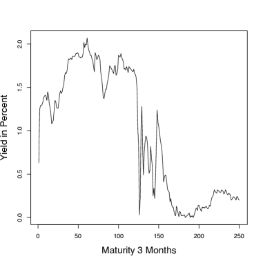
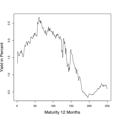
Figure 4.1. Yields over a one year period on US treasury bills with maturities of 3 and 12 months.

	HCCM	HCAD	VSC
3 Month	0.0243	0.0347	0.1072
12 Month	0.0545	0.0503	0.1073

Table 4.3. P–values for time series of yields in Figure 4.1.

5. Proofs of the asymptotic results

5.1. Proofs of the results of Section 2

Proof of Theorem 2.1. Let $S(k)=\sum_{\ell=1}^{k}e_{i}$ and $S(0)=0$. By the Abel’s summation formula we have

$$\sum_{\ell=1}^{k}u_{\ell}=\sum_{\ell=1}^{k}a(\ell/N)e_{\ell}=a(k/N)S(k)-\sum_{\ell=1}^{k-1}S(\ell)(a((\ell+1)/N)-a(\ell/N)),\;\;1\leq k\leq N.$$

Since under Assumption 2.3,

$$N^{-1/2}S(\lfloor Nt\rfloor)\;\;\stackrel{{\scriptstyle{\mathcal{D}}[0,1]}}{{\longrightarrow}}\;\;\sigma W(t),$$

by the Skorohod–Dudley–Wichura representation (cf. Shorack and Wellner (1986, p. 47)) we can define Wiener processes $W_{N}(t)$ such that

$$\max_{1\leq k\leq N}\left|S(k)-\sigma W_{N}(k)\right|=o_{P}(N^{1/2}).$$

Hence, by Assumption 2.2,

$$\max_{1\leq k\leq N} \left|\sum_{\ell=1}^{k}u_{\ell}-\sigma\left(a(k/N)W_{N}(k)-\sum_{\ell=1}^{k}W_{N}(\ell)(a((\ell+1)/N)-a(\ell/N))\right)\right|$$

$$\leq\max_{1\leq k\leq N}a(k/N)\left|S(k)-\sigma W_{N}(k)\right|$$

$$\hskip 28.45274pt+\max_{1\leq k\leq N}\left|\sum_{\ell=1}^{k-1}(S(\ell)-\sigma W_{N}(\ell))(a((\ell+1)/N)-a(\ell/N))\right|$$

$$=o_{P}(N^{1/2})\sup_{0\leq t\leq 1}a(t)+o_{P}(N^{1/2})\sum_{\ell=1}^{N-1}|a((\ell+1)/N)-a(\ell/N)|$$

$$=o_{P}(N^{1/2}).$$

By the Jordan decomposition theorem (cf. Hewitt and Stromberg (1969, p. 266)), there are two nondecreasing functions such that $a(x)=a_{1}(x)-a_{2}(x).$ Focusing on the function $a_{1}$, we can write

$$\sum_{\ell=1}^{k-1} W_{N}(\ell)(a_{1}((\ell+1)/N)-a_{1}(\ell/N))$$

$$=\sum_{\ell=1}^{k-1}W_{N}(\ell)\int_{\ell}^{\ell+1}da_{1}(x/N)$$

$$=\int_{0}^{k}W_{N}(x)da_{1}(x/N)+\sum_{\ell=1}^{k-1}\int_{\ell}^{\ell+1}(W_{N}(\ell)-W_{N}(x))da_{1}(x/N)$$

By the modulus of continuity of the Wiener process (cf. Lemma 1.2.1 of Csörgő and Révész (1981, p. 29)) we have that

$$\sup_{0\leq u\leq N}\sup_{0\leq x\leq 1}|W_{N}(u)-W_{N}(u+x)|=O_{P}((\log N)^{1/2}).$$

Integration by parts gives

$$W_{N}(k)a_{1}(k/N)-\int_{0}^{k}W_{N}(x)da_{1}(x/N)=\int_{0}^{k}a_{1}(x/N)dW_{N}(x)$$

and therefore

$$\left|a_{1}(k/N)W_{N}(k)-\sum_{\ell=1}^{k}W_{N}(\ell)(a_{1}((\ell+1)/N)-a_{1}(\ell/N))-\int_{0}^{k}a_{1}(x/N)dW_{N}(x)\right|$$

$$\hskip 85.35826pt=O_{P}((\log N)^{1/2}).$$

Similarly,

$$\left|a_{2}(k/N)W_{N}(k)-\sum_{\ell=1}^{k}W_{N}(\ell)(a_{2}((\ell+1)/N)-a_{2}(\ell/N))-\int_{0}^{k}a_{2}(x/N)dW_{N}(x)\right|$$

$$\hskip 85.35826pt=O_{P}((\log N)^{1/2}),$$

resulting in

$$\max_{1\leq k\leq N}\left|\sum_{\ell=1}^{k}u_{\ell}-\sigma\int_{0}^{k}a(x/N)dW_{N}(x)\right|=o_{P}(N^{1/2}).$$

Let

$$U_{N}(t)=\int_{0}^{t}a(x/N)dW_{N}(x),0\leq t\leq N.$$

It is easy to see that

$$\left\{U_{N}(t),0\leq t\leq N\right\}\stackrel{{\scriptstyle{\mathcal{D}}}}{{=}}\left\{W\left(\int_{0}^{t}a^{2}(x/N)dx\right),\quad 0\leq t\leq N\right\},$$

where $W(\cdot)$ is a Wiener process. Next we note that

$$\max_{0\leq k\leq N-1}\sup_{0\leq v\leq 1}\left|W\left(\int_{0}^{k}a^{2}(x/N)dx\right)-W\left(\int_{0}^{k+v}a^{2}(x/N)dx\right)\right|=O_{P}((\log N)^{1/2}),$$

since

$$\max_{0\leq k\leq N-1}\sup_{0\leq v\leq 1}\int_{k}^{k+v}a^{2}(x/N)dx\leq 4(a_{1}^{2}(1)+a_{2}^{2}(1)).$$

Thus, we conclude that

$$\sup_{0\leq t\leq 1}\left|N^{-1/2}\sum_{\ell=1}^{\lfloor Nt\rfloor}u_{\ell}-\frac{\sigma}{N^{1/2}}\int_{0}^{Nt}a(x/N)dW_{N}(x)\right|=o_{P}(1).$$

Since

$$\int_{0}^{Nt}a(x/N)dW_{N}(x)=\int_{0}^{t}a(z)dW_{N}(Nz),$$

by the scale transformation of the Wiener process we get that

$$\left\{N^{-1/2}\int_{0}^{Nt}a(x/N)dW_{N}(x),0\leq t\leq 1\right\}\stackrel{{\scriptstyle{\mathcal{D}}}}{{=}}\left\{\int_{0}^{t}a(x)dW(x),0\leq t\leq 1\right\}.$$

Computing the covariance function, one can easily verify that

$$\biggl{\{}\sigma\int_{0}^{t}a(x)dW(x),0\leq t\leq 1\biggl{\}}\stackrel{{\scriptstyle{\mathcal{D}}}}{{=}}\biggl{\{}W(b(t)),0\leq t\leq 1\biggl{\}},$$

completing the the proof of Lemma 2.1. ∎

Proof of Corollary 2.1. It follows immediately from Theorem 2.1. ∎

Proof of Corollary 2.2. The convergence in distribution in (2.2) is an immediate convergence of the continuous mapping theorem and Corollary 2.1 (cf. Billingsley (1968)).
The result in Corollary 2.1 can be restated by an application of the Skorohod–Dudley–Wichura representation (cf. Shorack and Wellner (1986, p. 47)) that there are Gaussian processes $\Gamma_{N}(t)$ distributed as $\Gamma(t)$ for each $N$ such that

(5.1) $$\sup_{0\leq t\leq 1}|Z_{N}(t)-\Gamma_{N}(t)|=o_{P}(1).$$

Let $0<\delta<1/2$. We write by the Cauchy–Schwartz inequality that

$$\left|\int_{1/N}^{1-1/N}\frac{Z_{N}^{2}(t)}{t(1-t)}dt-\int_{1/N}^{1-1/N}\frac{\Gamma^{2}_{N}(t)}{t(1-t)}dt\right|$$

$$\hskip 28.45274pt\leq\int_{1/N}^{1-1/N}\frac{|Z_{N}(t)-\Gamma_{N}(t)|}{(t(1-t))^{1/2-\delta}}\frac{|Z_{N}(t)|+|\Gamma_{N}(t)|}{t(1-t)^{1/2+\delta}}dt$$

$$\hskip 28.45274pt\leq 2\left(\int_{1/N}^{1-1/N}\frac{(Z_{N}(t)-\Gamma_{N}(t))^{2}}{(t(1-t))^{1-2\delta}}dt\right)^{1/2}$$

$$\hskip 56.62114pt\times\left(\int_{1/N}^{1-1/N}\frac{Z_{N}^{2}(t)}{(t(1-t))^{1+2\delta}}dt+\int_{1/N}^{1-1/N}\frac{\Gamma_{N}^{2}(t)}{(t(1-t))^{1+2\delta}}dt\right)^{1/2}.$$

It follows from (5.1) that

$$\int_{1/N}^{1-1/N}\frac{(Z_{N}(t)-\Gamma_{N}(t))^{2}}{(t(1-t))^{1-2\delta}}dt\leq\sup_{0\leq t\leq 1}|Z_{N}(t)-\Gamma_{N}(t)|\int_{0}^{1}(t(1-t))^{-1+2\delta}dt=o_{P}(1).$$

Next we show that

(5.2) $$\int_{1/N}^{1-1/N}\frac{Z_{N}^{2}(t)}{(t(1-t))^{1+2\delta}}dt=O_{P}(1)\;\;\;\mbox{and}\;\;\int_{1/N}^{1-1/N}\frac{\Gamma_{N}^{2}(t)}{(t(1-t))^{1+2\delta}}dt=O_{P}(1).$$

We note that $E\Gamma_{N}^{2}(t)=b(t)-2tb(t)+t^{2}b(1)=(b(t)-b(1))(1-2t)+(1-t)^{2}b(1)$ and therefore

(5.3) $$E\Gamma_{N}^{2}(t)\leq c_{1}t(1-t)\;\;\mbox{with some constant}\;\;c_{1}$$

resulting in

$$E\int_{1/N}^{1-1/N}\frac{\Gamma_{N}^{2}(t)}{(t(1-t))^{1+2\delta}}dt\leq c_{1}\int_{0}^{1}(t(1-t))^{-\delta}dt,$$

which proves the second half of (5.2). Using Assumption 2.2 and $|Ee_{i}e_{k}|=O((|k-i|+1)^{-\kappa})$ we get

$$E\left(\sum_{\ell=k}^{m}u_{\ell}\right)^{2}=\sum_{\ell=k}^{m}\sum_{\ell^{\prime}=k}^{m}a(\ell/N)a(\ell/N)Ee_{\ell}e_{\ell^{\prime}}\leq c_{2}\sum_{\ell=k}^{m}\sum_{\ell^{\prime}=k}^{m}|Ee_{\ell}e_{\ell^{\prime}}|\leq c_{3}(m-k)$$

with some constants $c_{2}$ and $c_{3}$. Hence $EZ^{2}_{N}(t)\leq c_{4}t(1-t)$ for all $1/N\leq t\leq 1-1/N$ which implies immediately that

$$E\int_{1/N}^{1-1/N}\frac{Z_{N}^{2}(t)}{(t(1-t))^{1+2\delta}}dt=O(1),$$

completing the proof of the first part of (5.2) via Markov’s inequality. We obtain from (5.3) that

$$\int_{0}^{1/N}\frac{\Gamma_{N}^{2}(t)}{t(1-t)}dt=o_{P}(1)\;\;\mbox{and}\;\;\int_{1-1/N}^{1}\frac{\Gamma_{N}^{2}(t)}{t(1-t)}dt=o_{P}(1),$$

which yields

$$\int^{1-1/N}_{1/N}\frac{\Gamma_{N}^{2}(t)}{t(1-t)}dt\;\;\stackrel{{\scriptstyle{\mathcal{D}}}}{{\to}}\;\;\int_{0}^{1}\frac{\Gamma^{2}(t)}{t(1-t)}dt,$$

since the distribution of $\Gamma_{N}(t)$ does not depend in $N$. ∎

Proof of Theorem 2.2. It follows from the definition of $X_{i}$ that

$$Z_{N}(t)=N^{-1/2}\left(\sum_{\ell=1}^{\lfloor Nt\rfloor}u_{\ell}-\frac{\lfloor Nt\rfloor}{N}\sum_{\ell=1}^{N}u_{\ell}\right)+N^{-1/2}d_{\lfloor Nt\rfloor}.$$

By Theorem 2.1 we have that

$$\sup_{0\leq t\leq 1}N^{-1/2}\left|\sum_{\ell=1}^{\lfloor Nt\rfloor}u_{\ell}-\frac{\lfloor Nt\rfloor}{N}\sum_{\ell=1}^{N}u_{\ell}\right|=O_{P}(1)$$

and by Assumption 2.5

$$\sup_{0\leq t\leq 1}\left|N^{-1/2}\left(\sum_{\ell=1}^{\lfloor Nt\rfloor}u_{\ell}-\frac{\lfloor Nt\rfloor}{N}\sum_{\ell=1}^{N}u_{\ell}\right)N^{-1/2}d_{\lfloor Nt\rfloor}\right|=O_{P}(N^{1/2}).$$

Hence (2.5) follows from the definition of $d(u)$ and Assumption 2.5 via the Lebesgue dominated convergence theorem (cf. Hewitt and Stromberg (1969, p. 172)).
Similar arguments can be used to prove (2.5) and therefore the details are omitted. ∎

Proof of Theorem 2.3. We have the usual representation

$$\hat{}\mbox{\boldmath${\beta}$}_{N}-\mbox{\boldmath${\beta}$}_{0}={\bf A}_{N}^{-1}{\bf Z}_{N},$$

where $\mbox{\boldmath${\beta}$}_{0}$ is the true parameter vector under $H_{0}$ and ${\bf Z}_{N}=[Z_{N}(1),\ldots,Z_{N}(p)]^{\top}$ with $Z_{N}(j)=\sum_{\ell=1}^{N}x_{\ell}(j)u_{\ell},\ \ 1\leq j\leq p$. Assumption 2.2 yields that $a(\cdot)$ is bounded and therefore by Assumptions 2.4 and 2.6 we conclude that

$$EZ_{N}(j) =\sum_{\ell=1}^{N}\sum_{k=1}^{N}E[x_{\ell}(j)x_{k}(j)u_{\ell}u_{k}]\leq\sum_{\ell=1}^{N}\sum_{k=1}^{N}|E[x_{\ell}(j)x_{k}(j)]||E[u_{\ell}u_{k}]|$$

$$\leq O(1)\sum_{\ell=1}^{N}\sum_{k=1}^{N}(Ex^{2}_{\ell}(j)Ex^{2}_{k}(j))^{1/2}(|k-\ell|+1)^{-\kappa}=O(N).$$

Since $A^{-1}_{N}=O_{P}(1/N)$, we obtain that

(5.4) $$N^{1/2}\|\hat{}\mbox{\boldmath${\beta}$}_{N}-\mbox{\boldmath${\beta}$}_{0}\|=O_{P}(1).$$

Using Assumption 2.6 we get via the ergodic theorem that

(5.5) $$\frac{1}{N}\max_{1\leq i\leq N}\left\|\sum_{j=1}^{i}{\bf x}_{j}-\frac{i}{N}\sum_{j=1}^{N}{\bf x}_{j}\right\|=o_{P}(1).$$

It follows from (5.4) and (5.5) that

$$N^{-1/2}\max_{1\leq i\leq N}\left|\left(\sum_{j=1}^{i}\hat{u}_{j}-\frac{i}{N}\sum_{j=1}^{N}\hat{u}_{j}\right)-\left(\sum_{j=1}^{i}{u}_{j}-\frac{i}{N}\sum_{j=1}^{N}{u}_{j}\right)\right|=o_{P}(1),$$

completing the proof of Theorem 2.3. ∎

Proof of Theorem 2.4. First we write

$$L_{N}(\mbox{\boldmath${\theta}$})=\sum_{i=1}^{N}u_{i}^{2}+V_{N}(\mbox{\boldmath${\theta}$}),\quad V_{N}(\mbox{\boldmath${\theta}$})=2\sum_{i=1}^{N}u_{i}(h({\bf x}_{i},\mbox{\boldmath${\theta}$}_{0})-h({\bf x}_{i},\mbox{\boldmath${\theta}$}))+\sum_{i=1}^{N}(h({\bf x}_{i},\mbox{\boldmath${\theta}$}_{0})-h({\bf x}_{i},\mbox{\boldmath${\theta}$}))^{2}$$

and the location of the minimum of $L_{N}$ and $V_{N}$ is the same. Using Assumption 2.8 and the ergodic we get that

$$\sup_{\mbox{\boldmath${\theta}$}\in{\mbox{\boldmath${\Theta}$}}}\left|\frac{1}{N}L_{N}(\mbox{\boldmath${\theta}$})-V(\mbox{\boldmath${\theta}$})\right|=o(1)\;\;\;\;a.s.,\;\;\;\;\mbox{where}\;\;\;V(\mbox{\boldmath${\theta}$})=E(h({\bf x}_{0},\mbox{\boldmath${\theta}$}_{0})-h({\bf x}_{0},\mbox{\boldmath${\theta}$}))^{2}.$$

Since $V(\mbox{\boldmath${\theta}$})$ has a unique maximum at $\mbox{\boldmath${\theta}$}_{0}$, standard arguments yield (c.f. Pfanzagl (1994)) that

(5.6) $$\hat{\mbox{\boldmath${\theta}$}}_{N}\to\mbox{\boldmath${\theta}$}_{0}\;\;\;\;a.s.$$

Next we observe that

$$\frac{\partial}{\partial\mbox{\boldmath${\theta}$}}L_{N}(\hat{\mbox{\boldmath${\theta}$}}_{N})={\bf 0}.$$

Also, by the ergodic theorem and Assumption 2.8 we have that

$$\sup_{\mbox{\boldmath${\theta}$}\in{\mbox{\boldmath${\Theta}$}}}\left\|\frac{\partial^{2}}{\mbox{\boldmath${\theta}$}^{2}}\frac{1}{N}L_{N}(\mbox{\boldmath${\theta}$})-\frac{\partial^{2}}{\mbox{\boldmath${\theta}$}^{2}}V(\mbox{\boldmath${\theta}$})\right\|=o(1)\;\;a.s.,$$

$\partial^{2}V(\mbox{\boldmath${\theta}$})/\mbox{\boldmath${\theta}$}^{2}$ is continuous on ${\Theta}$ and $\partial^{2}V(\mbox{\boldmath${\theta}$}_{0})/\mbox{\boldmath${\theta}$}^{2}$ is nonsingular since $V(\theta)$ has a unique minimum at $\mbox{\boldmath${\theta}$}_{0}$. Applying the mean value theorem coordinatewise we obtain that

$$\frac{\partial}{\partial\mbox{\boldmath${\theta}$}}L_{N}(\mbox{\boldmath${\theta}$}_{0})=\frac{\partial}{\partial\mbox{\boldmath${\theta}$}}L_{N}(\mbox{\boldmath${\theta}$}_{0})-\frac{\partial}{\partial\mbox{\boldmath${\theta}$}}L_{N}(\hat{\mbox{\boldmath${\theta}$}}_{N})={\bf G}_{N}(\mbox{\boldmath${\theta}$}_{0}-\hat{\mbox{\boldmath${\theta}$}}_{N})^{\top}$$

and

$$\frac{1}{N}{\bf G}_{N}\to\frac{\partial^{2}}{\mbox{\boldmath${\theta}$}^{2}}V(\mbox{\boldmath${\theta}$}_{0})\;\;\;a.s.$$

Following the proof of Theorem 2.3 one can verify that

$$E\left\|\frac{\partial}{\partial\mbox{\boldmath${\theta}$}}L_{N}(\mbox{\boldmath${\theta}$}_{0})\right\|^{2}=O(N)$$

and therefore

(5.7) $$N^{1/2}\left\|\hat{\mbox{\boldmath${\theta}$}}_{N}-\mbox{\boldmath${\theta}$}_{0}\right\|=O_{P}(1).$$

Using a two term Taylor expansion with the ergodic theorem and (5.7) we get that

$$\sum_{j=1}^{i}\hat{u}_{j}-\frac{i}{N}\sum_{j=1}^{N}\hat{u}_{j}=\sum_{j=1}^{i}{u}_{j}-\frac{i}{N}\sum_{j=1}^{N}{u}_{j}+{\mathcal{R}}_{i,1}+{\mathcal{R}}_{i,2}$$

with

$${\mathcal{R}}_{i,1}=\left(\sum_{j=1}^{i}\frac{\partial}{\mbox{\boldmath${\theta}$}}{h}({\bf x}_{j},\mbox{\boldmath${\theta}$}_{0})-\frac{i}{N}\sum_{j=1}^{N}\frac{\partial}{\mbox{\boldmath${\theta}$}}{h}({\bf x}_{j},\mbox{\boldmath${\theta}$}_{0})\right)^{\top}(\mbox{\boldmath${\theta}$}_{0}-\hat{\mbox{\boldmath${\theta}$}}_{N})$$

and $N^{-1/2}\max_{1\leq i\leq N}|{\mathcal{R}}_{i,2}|=o_{P}(1)$. Repeating the argument used in the proof of Theorem 2.3, by (5.7) and the ergodic theorem we obtain that $N^{-1/2}\max_{1\leq i\leq N}|{\mathcal{R}}_{i,1}|=o_{P}(1)$. Hence the proof is complete. ∎

5.2. Proofs of the results in Section 3

Lemma 5.1.

If Assumptions 2.1–2.3, 2.5, 3.1 are satisfied and $\{e_{i},-\infty<i<\infty\}$ is a stationary and ergodic sequence with $Ee_{0}=0$ and $Ee^{2}_{0}=\sigma^{2}$, then we have that

(5.8) $$\max_{1\leq k\leq N}\left|H_{N}(k/N)-\frac{1}{N}\left(\sum_{\ell=1}^{k}u^{2}_{\ell}+\sum_{\ell=1}^{k}(\mu_{\ell}-\bar{\mu})^{2}\right)\right|=O_{P}(N^{-1/2}\log N)$$

and

(5.9) $$\int_{0}^{1}\left(H_{N}(u)-(b(u)+g(u))\right)^{2}dt=o_{P}(1).$$

Proof.

It is easy to see that

$$NH_{N}(k/N)= \sum_{\ell=1}^{k}u^{2}_{\ell}+\sum_{\ell=1}^{k}(\mu_{\ell}-\bar{\mu})^{2}+2\sum_{\ell=1}^{k}u_{\ell}(\mu_{\ell}-\bar{\mu})+2(\bar{\mu}-\bar{X}_{N})\sum_{\ell=1}^{k}u_{\ell}$$

$$\hskip 28.45274pt+2(\bar{\mu}-\bar{X}_{N})\sum_{\ell=1}^{k}(\mu_{\ell}-\bar{\mu})+k(\bar{\mu}-\bar{X}_{N})^{2}.$$

It follows from Theorem 2.1 that

$$\bar{X}_{N}-\bar{\mu}=\frac{1}{N}\sum_{\ell=1}^{N}u_{\ell}=O_{P}(N^{-1/2})$$

and

$$\max_{1\leq k\leq N}\left|\sum_{\ell=1}^{k}u_{\ell}\right|=O_{P}(N^{1/2})$$

and therefore

$$\max_{1\leq k\leq N}\left|(\bar{\mu}-\bar{X}_{N})\sum_{\ell=1}^{k}u_{\ell}\right|=O_{P}(1),\quad\max_{1\leq k\leq N}\left|(\bar{\mu}-\bar{X}_{N})\sum_{\ell=1}^{k}(\mu_{\ell}-\bar{\mu})\right|=O_{P}(N^{1/2})$$

and

$$\max_{1\leq k\leq N}k(\bar{\mu}-\bar{X}_{N})^{2}=O_{P}(1).$$

Using Assumptions 2.2, 2.5 and 3.1, we get that

$$E\left(\sum_{\ell=m}^{k}u_{\ell}(\mu_{\ell}-\bar{\mu})\right)^{2}\leq c_{1}(k-m)\;\;\mbox{for all}\;\;1\leq k\leq m\leq N$$

with some $c_{1}$ and therefore by Menshov’s inequality (cf. Billingsley (1968, p. 102)) that

$$\max_{1\leq k\leq N}\left|\sum_{\ell=1}^{k}u_{\ell}(\mu_{\ell}-\bar{\mu})\right|=O_{P}(N^{1/2}\log N).$$

Next we show that

(5.10) $$\max_{1\leq k\leq N}\left|\sum_{\ell=1}^{k}(u^{2}_{\ell}-\sigma^{2}a^{2}(\ell/N))\right|=o_{P}(N).$$

Set

$$\mbox{$\mathcal{S}$}(0)=0\;\;\mbox{ and }\;\;\mbox{$\mathcal{S}$}(k)=\sum_{\ell=1}^{k}(e_{\ell}^{2}-\sigma^{2}).$$

By Abel’s summation formula we have

$$\sum_{\ell=1}^{k}(u^{2}_{\ell}-\sigma^{2}a^{2}(\ell/N)) =\sum_{\ell=1}^{k}a^{2}(\ell/N)(\mbox{$\mathcal{S}$}(\ell)-\mbox{$\mathcal{S}$}(\ell-1))$$

$$=\mbox{$\mathcal{S}$}(N)a^{2}(1)-\sum_{\ell=1}^{k-1}\mbox{$\mathcal{S}$}_{\ell}(a^{2}((\ell+1)/N)-a^{2}(\ell/N)).$$

It follows from the ergodic theorem (cf. Breiman (1968, p. 118) that

$$\lim_{k\to\infty}\frac{1}{k}\mbox{$\mathcal{S}$}(k)=0\quad\mbox{a.s.}$$

For any $\delta>0$, there is a random variable $k^{*}=k^{*}(\omega)$ such that $|\mbox{$\mathcal{S}$}(k)|\leq\delta k$ if $k\leq k^{*}$ and therefore for $k>k^{*}$

$$\frac{1}{N} \left|\sum_{\ell=1}^{k-1}\mbox{$\mathcal{S}$}_{\ell}(a^{2}((\ell+1)/N)-a^{2}(\ell/N))\right|$$

$$\leq\frac{1}{N}\sum_{\ell=1}^{k^{*}}|\mbox{$\mathcal{S}$}_{\ell}(a^{2}((\ell+1)/N)-a^{2}(\ell/N))|+\frac{1}{N}\sum_{\ell=k^{*}+1}^{k-1}\frac{|\mbox{$\mathcal{S}$}_{\ell}|}{\ell}\ell|a^{2}((\ell+1)/N)-a^{2}(\ell/N)|$$

$$=o_{P}(1)+\delta\sum_{\ell=1}^{N-1}|a^{2}((\ell+1)/N)-a^{2}(\ell/N)|.$$

It follows from Assumption 2.2 that $a^{2}(t)$ also has bounded variation on $[0,1]$. Since $\delta$ can be as small as we want, the proof of (5.10) is complete. Observing that

$$\int_{0}^{1}\left(\frac{1}{N}\sum_{\ell=1}^{\lfloor Nt\rfloor}a^{2}(\ell/N)-\int_{0}^{t}a^{2}(s)ds\right)^{2}dt=o(1),$$

the proof of (5.9) is complete. ∎

Proof of Theorem 3.1. It is an immediate consequence of Lemma 5.1 and the definition of $\widehat{C}_{N}(t,s)$. ∎

It follows from the definition of $\hat{\gamma}_{N;k,\ell}$ that for $\ell\geq 0$

$$N\hat{\gamma}_{N;k,\ell}=r_{k,\ell,1}+\ldots+r_{k,\ell,9},$$

where

$$r_{k,\ell,1}=\sum_{i=1}^{k-\ell}(X_{i}-\mu_{i})(X_{i+\ell}-\mu_{i+\ell}), r_{k,\ell,2}=(\bar{\mu}-\bar{X}_{N})\sum_{i=1}^{k-\ell}(X_{i}-\mu_{i})$$

$$r_{k,\ell,3}=(\bar{\mu}-\bar{X}_{N})\sum_{i=1}^{k-\ell}(X_{i+\ell}-\mu_{i+\ell}), r_{k,\ell,4}=(k-\ell)(\bar{\mu}-\bar{X}_{N})^{2}$$

$$r_{k,\ell,5}=\sum_{i=1}^{k-\ell}(X_{i}-\mu_{i})(\mu_{i+\ell}-\bar{\mu}), r_{k,\ell,6}=\sum_{i=1}^{k-\ell}(X_{i+\ell}-\mu_{i+\ell})(\mu_{i}-\bar{\mu})$$

$$r_{k,\ell,7}=(\bar{\mu}-\bar{X}_{N})\sum_{i=1}^{k-\ell}(\mu_{i}-\bar{\mu}), r_{k,\ell,8}=(\bar{\mu}-\bar{X}_{N})\sum_{i=1}^{k-\ell}(\mu_{i+\ell}-\bar{\mu})$$

and

$$r_{k,\ell,9}=\sum_{i=1}^{k-\ell}(\mu_{i}-\bar{\mu})(\mu_{i+\ell}-\bar{\mu}).$$

Lemma 5.2.

If $H_{0}$, Assumptions 2.1, 2.2 and 3.2–3.4 are satisfied, then we have that

$$\int_{0}^{1}(\hat{g}_{N}(t)-b(t))^{2}=o_{P}(1).$$

Proof.

It is easy to see that

$$Er_{k,\ell,1}=\sum_{i=1}^{k-\ell}Eu_{i}u_{i+\ell}=\sum_{i=1}^{k-\ell}a(i/N)a((i+\ell)/N)r(\ell),\;\;\mbox{where}\;r(\ell)=Ee_{0}e_{\ell},$$

resulting in

$$E\sum_{\ell=1}^{k}K(\ell/h)\frac{1}{N}r_{k,\ell,1}=\frac{1}{N}\sum_{\ell=1}^{k}K(\ell/h)r(\ell)\sum_{i=1}^{k-\ell}a(i/N)a((i+\ell)/N).$$

Let $M$ be a positive integer. We have for $k\geq M$ that

$$F_{N}(k) =\biggl{|}\sum_{\ell=1}^{k}K(\ell/h)r(\ell)\frac{1}{N}\sum_{i=1}^{k-\ell}a(i/N)a((i+\ell)/N)-\sum_{\ell=1}^{M}K(\ell/h)r(\ell)\frac{1}{N}\sum_{i=1}^{k-\ell}a(i/N)a((i+\ell)/N)\biggl{|}$$

$$\leq c_{1}\sum_{\ell=M+1}^{\infty}|r(\ell)|$$

with some constant $c_{1}$ since by Assumptions 2.2 and 3.2 $K$ and $a$ are bounded functions. If $1\leq k\leq M$, then

$$\Biggl{|}\sum_{\ell=1}^{k}K(\ell/h)r(\ell)\frac{1}{N}\sum_{i=1}^{k-\ell}a(i/N)a((i+\ell)/N)\Biggl{|}\leq c_{2}\frac{M^{2}}{N}.$$

Hence we have

(5.11) $$\max_{1\leq k\leq N}|F_{N}(k)|\leq c_{1}\sum_{\ell=M+1}^{\infty}|r(\ell)|+c_{2}\frac{M^{2}}{N}.$$

Using Assumptions 2.2 and 3.2 we have

(5.12) $$\max_{1\leq k\leq N}\Biggl{|}\sum_{\ell=1}^{M}(K(\ell/h)-1)r(\ell)\frac{1}{N}\sum_{i=1}^{k-\ell}a(i/N)a((i+\ell)/N)\Biggl{|}\leq c_{3}\frac{M^{2}}{h}$$

with some constant $c_{3}$ and

(5.13) $$\max_{1\leq k\leq N} \Biggl{|}\sum_{\ell=1}^{M}r(\ell)\frac{1}{N}\left(\sum_{i=1}^{k-\ell}a(i/N)a((i+\ell)/N)-\sum_{i=1}^{k}a(i/N)a((i+\ell)/N)\right)\Biggl{|}$$

$$\leq c_{4}\left(\sum_{\ell=1}^{\infty}|r(\ell)|\right)\frac{M}{N}.$$

Next we note that

(5.14) $$\max_{1\leq k\leq N} \left|\sum_{\ell=1}^{M}r(\ell)\frac{1}{N}\sum_{i=1}^{k}a(i/N)(a((i+\ell)/N)-a(i/N))\right|$$

$$\leq c_{5}\frac{1}{N}\max_{1\leq\ell\leq N}\sum_{i=1}^{N}|a((i+\ell)/N)-a(i/N)|$$

$$\leq c_{6}\frac{M}{N},$$

by Assumption 2.2, where $c_{5}$ and $c_{6}$ are constants and $a(u)=0$ for $u>1$. Finally,

(5.15) $$\max_{1\leq k\leq N}\left|\sum_{\ell=1}^{M}r(\ell)\frac{1}{N}\sum_{i=1}^{k}a^{2}(i/N)-\sum_{\ell=1}^{\infty}r(\ell)\frac{1}{N}\sum_{i=1}^{k}a^{2}(i/N)\right|\leq c_{7}\sum_{\ell=M+1}^{\infty}|r(\ell)|,$$

with some constant $c_{7}$. Putting together (5.11)–(5.15) we conclude that

$$\limsup_{N\to\infty}\left|E\sum_{\ell=1}^{k}K(\ell/h)\frac{1}{N}r_{k,\ell,1}-\left(\sum_{\ell=1}^{\infty}r(\ell)\right)\frac{1}{N}\sum_{i=1}^{k}a^{2}(i/N)\right|\leq(c_{1}+c_{7})\sum_{M+1}^{\infty}|r(\ell)|,$$

and since we can take $M$ as large as we want to we obtain

$$\lim_{N\to\infty}\left|E\sum_{\ell=1}^{k}K(\ell/h)\frac{1}{N}r_{k,\ell,1}-\left(\sum_{\ell=1}^{\infty}r(\ell)\right)\frac{1}{N}\sum_{i=1}^{k}a^{2}(i/N)\right|=0.$$

Next we show that

(5.16) $$\frac{1}{N}\sum_{k=1}^{N}\left(\sum_{\ell=1}^{k}K(h/\ell)\frac{1}{N}(r_{k,\ell,1}-Er_{k,\ell,1})\right)^{2}=o_{P}(1).$$

We observe that by the stationarity of the $e_{i}$’s and Assumptions 2.2 and 3.2

$$E\frac{1}{N} \sum_{k=1}^{N}\left(\sum_{\ell=1}^{k}K(h/\ell)\frac{1}{N}(r_{k,\ell,1}-Er_{k,\ell,1})\right)^{2}$$

$$=\frac{1}{N^{3}}\sum_{k=1}^{N}\sum_{\ell=1}^{k}\sum_{\ell^{\prime}=1}^{k}K(\ell/h)K(\ell^{\prime}/h)\sum_{i=1}^{k-\ell}\sum_{j=1}^{k-\ell^{\prime}}a(\ell/N)a((\ell+i)/N)a(j/N)a((j+\ell^{\prime})/N)$$

$$\hskip 28.45274pt\times(Ee_{i}e_{i+\ell}e_{j}e_{j+\ell^{\prime}}-r(\ell)r(\ell^{\prime}))$$

$$\leq c_{8}\frac{1}{N^{3}}\sum_{k=1}^{N}\sum_{\ell=1}^{ch}\sum_{\ell^{\prime}=1}^{ch}k\sum_{j=1}^{k}|Ee_{0}e_{\ell}e_{j}e_{j+\ell^{\prime}}-r(\ell)r(\ell^{\prime})|$$

$$\leq c_{8}\frac{1}{N^{2}}\sum_{k=1}^{N}\sum_{\ell=1}^{ch}\sum_{\ell^{\prime}=1}^{ch}\sum_{j=1}^{k}|Ee_{0}e_{\ell}e_{j}e_{j+\ell^{\prime}}-r(\ell)r(\ell^{\prime})|.$$

Let

$$G_{1,k} =\{(j,\ell,\ell^{\prime}):\;ch+1\leq j\leq k,1\leq\ell,\ell^{\prime}\leq ch\}$$

$$G_{2,k} =\{(j,\ell,\ell^{\prime}):\;1\leq j\leq ch,1\leq\ell,\ell^{\prime}\leq ch\}$$

and define

$$Q_{1,k}=\sum_{(j,\ell,\ell^{\prime})\in G_{1,k}}|Ee_{0}e_{\ell}e_{j}e_{j+\ell^{\prime}}-r(\ell)r(\ell^{\prime})|,\quad Q_{2,k}=\sum_{(j,\ell,\ell^{\prime})\in G_{1,k}}|Ee_{0}e_{\ell}e_{j}e_{j+\ell^{\prime}}-r(\ell)r(\ell^{\prime})|.$$

Next we define

$$\bar{e}_{j,j-\ell-1}=f(\varepsilon_{j},\varepsilon_{j-1},\ldots,\varepsilon_{\ell+1},\varepsilon_{\ell}^{\prime},\varepsilon_{\ell-1}^{\prime},\ldots)$$

and

$$\bar{e}_{j+\ell^{\prime},j+\ell^{\prime}-\ell-1}=f(\varepsilon_{j+\ell^{\prime}},\varepsilon_{j+\ell^{\prime}-1},\ldots,\varepsilon_{\ell+1},\varepsilon_{\ell}^{\prime},\varepsilon_{\ell-1}^{\prime},\ldots),$$

where $\varepsilon_{v}^{\prime},-\infty<v<\infty$ are independent copies of $\varepsilon_{0}$, independent of $\varepsilon_{j},-\infty<j<\infty$. It follows from Assumption 3.4 that $(e_{0},e_{\ell})$ is independent of $(\bar{e}_{j,j-\ell-1},\bar{e}_{j+\ell^{\prime},j+\ell^{\prime}-\ell-1})$. Also, according to the construction the vectors $(e_{j},e_{j+\ell^{\prime}})$ and $(\bar{e}_{j,j-\ell-1},\bar{e}_{j+\ell^{\prime},j+\ell^{\prime}-\ell-1})$ have the same distribution. Note that $Ee_{0}e_{\ell}\bar{e}_{j,j-\ell-1}\bar{e}_{j+\ell^{\prime},j+\ell^{\prime}-\ell-1}=E[e_{0}e_{\ell}]E[\bar{e}_{j,j-\ell-1}\bar{e}_{j+\ell^{\prime},j+\ell^{\prime}-\ell-1}]=r(\ell)r(\ell^{\prime})$. Hence

$$Ee_{0}e_{\ell}e_{j}e_{j+\ell^{\prime}}-r(\ell)r(\ell^{\prime})=Ee_{0}e_{\ell}[e_{j}e_{j+\ell^{\prime}}-\bar{e}_{j,j-\ell-1}\bar{e}_{j+\ell^{\prime},j+\ell^{\prime}-\ell-1}].$$

It follows from Assumption 3.4

$$(E(e_{j}-\bar{e}_{j,j-\ell-1})^{4})^{1/4}\leq c_{8}(j-\ell)^{-\alpha}\;\;\mbox{and}\;\;(E(e_{j+\ell^{\prime}}-\bar{e}_{j+\ell^{\prime},j+\ell^{\prime}-\ell-1})^{4})^{1/4}\leq c_{8}(j+\ell^{\prime}-\ell)^{-\alpha}$$

with some constant $c_{8}$ for all $(j,\ell,\ell^{\prime})\in G_{1,k}$. Hence the cauchy–Schwartz inequality yields

$$|E e_{0}e_{\ell}[e_{j}e_{j+\ell^{\prime}}-\bar{e}_{j,j-\ell-1}\bar{e}_{j+\ell^{\prime},j+\ell^{\prime}-\ell-1}]|$$

$$E|e_{0}e_{\ell}e_{j}[e_{j+\ell^{\prime}}-\bar{e}_{j+\ell^{\prime},j+\ell^{\prime}-\ell-1}]|+E|e_{0}e_{\ell}\bar{e}_{j+\ell^{\prime},j+\ell^{\prime}-\ell-1}[e_{j}-\bar{e}_{j,j-\ell-1}]|$$

$$\leq(Ee_{0}^{4}e_{\ell}^{4}e_{j}^{4}E[e_{j+\ell^{\prime}}-\bar{e}_{j+\ell^{\prime},j+\ell^{\prime}-\ell-1}]^{4})^{1/4}+(Ee_{0}^{4}e_{\ell}^{4}\bar{e}_{j+\ell^{\prime},j+\ell^{\prime}-\ell-1}^{4}E[e_{j}-\bar{e}_{j,j-\ell-1}]^{4})^{1/4}$$

$$\leq c_{8}(Ee_{0}^{4})^{3/4}((j-\ell)^{-\alpha}+(j+\ell^{\prime}-\ell)^{-\alpha})$$

$$\leq 2c_{8}(Ee_{0}^{4})^{3/4}(j-\ell)^{-\alpha}$$

for all $(j,\ell,\ell^{\prime})\in G_{1,k}$. Thus we get with $c_{9}=2c_{8}(Ee_{0}^{4})^{3/4}$ that

$$Q_{1,k}\leq c_{9}\sum_{(j,\ell,\ell^{\prime})\in G_{1,k}}(j-\ell)^{-\alpha}\leq c_{10}h\int_{ch+1}^{\infty}\int_{1}^{ch}(x-y)^{-\alpha}dydx\leq c_{11}h$$

with some constants $c_{10}$ and $c_{11}$.
We note that

$$Q_{2,k}\leq\sum_{(j,\ell,\ell^{\prime})\in G_{2,k}}|E[e_{0}e_{\ell}e_{j}e_{j+\ell^{\prime}}]|+\sum_{(j,\ell,\ell^{\prime})\in G_{2,k}}|E[e_{0}e_{\ell}]E[e_{j}e_{j+\ell^{\prime}}]|$$

and

$$\sum_{(j,\ell,\ell^{\prime})\in G_{2,k}}|E[e_{0}e_{\ell}]E[e_{j}e_{j+\ell^{\prime}}]|\leq ch\left(\sum_{\ell=1}^{\infty}|Ee_{0}e_{\ell}|\right)^{2}.$$

Let $e_{j,m}$ be the random variables defined in Assumption 3.4. We get for all $0\leq s\leq t\leq v\leq 2ch$ that

$$e_{0} e_{s}e_{t}e_{v}=e_{0}e_{s,s}(e_{t}-e_{t,t-s})(e_{v}-e_{v,v-t})+e_{0}e_{s,s}(e_{t}-e_{t,t-s})e_{v,v-t}+e_{0}e_{s,s}e_{t,t-s}(e_{v}-e_{v,v})$$

$$+e_{0}e_{s,s}e_{t,t-s}e_{v,v}+e_{0}(e_{s}-e_{s,s})(e_{t}-e_{t,t-s})e_{v}+e_{0}(e_{s}-e_{s,s})e_{t,t-s}e_{v,v-t}$$

$$+e_{0}(e_{s}-e_{s,s})e_{t,t-s}(e_{v}-e_{v,v-t}).$$

The definition of $e_{j,m}$ yields that $e_{v,v-t}$ is independent of $e_{0}e_{s,s}(e_{t}-e_{t,t-s})$, $e_{0}$ is independent of $e_{s,s}e_{t,t-s}e_{v,v}$ and $e_{v,v-t}$ is independent of $e_{0}(e_{s}-e_{s,s})e_{t,t-s}$ and therefore

$$E[e_{0}e_{s,s}(e_{t}-e_{t,t-s})e_{v,v-t}]=0,\;\;E[e_{0}e_{s,s}e_{t,t-s}e_{v,v}]=0\;\;\mbox{and}\;\;E[e_{0}(e_{s}-e_{s,s})e_{t,t-s}e_{v,v-t}]=0.$$

Using Assumption 3.4 we obtain that

$$\sum_{1\leq s\leq t\leq v\leq 2ch} E|e_{0}e_{s,s}(e_{t}-e_{t,t-s})(e_{v}-e_{v,v-t})|$$

$$\leq(Ee_{0}^{4})^{1/2}\sum_{1\leq s\leq t\leq v\leq 2ch}(E(e_{t}-e_{t,t-s})^{4})^{1/4}(E(e_{v}-e_{v,v-t})^{4})^{1/4}$$

$$=O(h).$$

Similarly,

$$\sum_{1\leq s\leq t\leq v\leq 2ch}E|e_{0}(e_{s}-e_{s,s})(e_{t}-e_{t,t-s})e_{v}|=O(h)$$

and

$$\sum_{1\leq s\leq t\leq v\leq 2ch}E|e_{0}(e_{s}-e_{s,s})e_{t,t-s}(e_{v}-e_{v,v-t})|=O(h)$$

and

$$\sum_{1\leq s\leq t\leq v\leq 2ch}E|e_{0}e_{s,s}e_{t,t-s}(e_{v}-e_{v,v})|=O(1)\int_{0}^{2ch}\int_{s}^{2ch}\int_{t}^{2ch}v^{-\alpha}dvdtds=O(h).$$

Thus we conclude

$$Q_{2,k}\leq c_{l2}h,$$

which completes the proof of

$$E\frac{1}{N}\sum_{k=1}^{N}\left(\sum_{\ell=1}^{k}K(h/\ell)\frac{1}{N}(r_{k,\ell,1}-Er_{k,\ell,1})\right)^{2}=O(h/N)$$

and therefore (5.16) follows via Markov’s inequality.
Theorem 2.1 yields that

$$\max_{1\leq k\leq N}\left|\sum_{\ell=1}^{k-1}K(\ell/h)\frac{1}{N}r_{k,\ell,2}\right|\leq\frac{ch}{N^{2}}\left|\sum_{i=1}^{N}u_{i}\right|\max_{|u|\leq c}|K(u)|\max_{1\leq k\leq N}\left|\sum_{i=1}^{k}u_{i}\right|=O_{P}(h/N).$$

Similar argument gives

$$\max_{1\leq k\leq N}\left|\sum_{\ell=1}^{k-1}K(\ell/h)\frac{1}{N}r_{k,\ell,3}\right|=O_{P}(h/N).$$

Theorem 2.1 and Assumption 3.2 yield

$$\max_{1\leq k\leq N}\left|\sum_{\ell=1}^{k}K(\ell/N)\frac{1}{N}r_{k,\ell,4}\right|\leq\frac{1}{N^{3}}\left(\sum_{i=1}^{N}u_{i}\right)^{2}\max_{1\leq k\leq N}\left|\sum_{\ell=1}^{k}K(\ell/h)(k-\ell)\right|=O_{P}(h/N).$$

Since $r_{k,\ell,5}=r_{k,\ell,6}=r_{k,\ell,7}=r_{k,\ell,8}=r_{k,\ell,9}=0$ under $H_{0}$ we proved that

(5.17) $$\int_{0}^{1}\left(\sum_{\ell=1}^{\lfloor Nu\rfloor-1}K(\ell/h)\hat{\gamma}_{N,\lfloor Nu\rfloor,\ell}-\sum_{\ell=1}^{\infty}r(\ell)\int_{0}^{u}a^{2}(v)dv\right)^{2}du=o_{P}(1).$$

Similar arguments show that

(5.18) $$\int_{0}^{1}\Biggl{(}\sum^{0}_{\ell=-(\lfloor Nu\rfloor-1)}K(\ell/h)\hat{\gamma}_{N,\lfloor Nu\rfloor,\ell}-\sum^{0}_{\ell=-\infty}r(\ell)\int_{0}^{u}a^{2}(v)dv\Biggl{)}^{2}du=o_{P}(1).$$

Now Lemma 5.2 follows from (5.17) and (5.18). ∎

Lemma 5.3.

If $H_{A}$, Assumptions 2.1, 2.2 and 3.2–3.4 are satisfied, then we have

$$\int_{0}^{1}\hat{g}_{N}^{2}(u)du=O_{P}(h^{2}).$$

If in addition, Assumption

$$\int_{0}^{1}\left(\frac{1}{h}\hat{g}_{N}(u)-g(u)\int_{-c}^{c}K(v)dv\right)^{2}du=o_{P}(1).$$

Proof.

Following the proof of Theorem 2.1 one can show that

$$\max_{1\leq k\leq N}\max_{1\leq\ell<k}\left|\sum_{i=1}^{k-\ell}(X_{i}-\mu_{i})(\mu_{i+\ell}-\bar{\mu})\right|=\max_{1\leq k\leq N}\max_{1\leq\ell<k}\left|\sum_{i=1}^{k-\ell}u_{i}(\mu_{i+\ell}-\bar{\mu})\right|=O_{P}(N^{1/2}),$$

and therefore

$$\max_{1\leq k\leq N}\left|\sum_{\ell=1}^{k}K(\ell/h)\frac{1}{N}r_{k,\ell,5}\right|=O_{P}(h/N^{1/2}).$$

Similarly,

$$\max_{1\leq k\leq N}\left|\sum_{\ell=1}^{k}K(\ell/h)\frac{1}{N}r_{k,\ell,6}\right|=O_{P}(h/N^{1/2}).$$

Combining Theorem 2.1 and Assumption 2.5 we conclude

$$\max_{1\leq k\leq N}\left|\sum_{\ell=1}^{k}K(\ell/h)\frac{1}{N}r_{k,\ell,7}\right| \leq\frac{1}{N^{3}}\left(\sum_{i=1}^{N}u_{i}\right)^{2}\max_{1\leq k\leq N}\left|\sum_{\ell=1}^{k}K(\ell/h)\sum_{j=1}^{k-\ell}(\mu_{i}-\bar{\mu})\right|$$

$$=O_{P}(h/N)$$

and

$$\max_{1\leq k\leq N}\left|\sum_{\ell=1}^{k}K(\ell/h)\frac{1}{N}r_{k,\ell,8}\right|=O_{P}(h/N)$$

We note that by Assumptions 2.5 and 3.2

$$\max_{1\leq k\leq N}\left|\sum_{\ell=1}^{k-1}K(\ell/h)\frac{1}{N}\sum_{i=1}^{k-\ell}(\mu_{i}-\bar{\mu})(\mu_{i+\ell}-\bar{\mu})\right|=O_{(}h),$$

and therefore by the proof of Lemma 5.2 we get

(5.19) $$\int_{0}^{1}\left(\sum_{\ell=1}^{\lfloor Nu\rfloor-1}K(\ell/h)\hat{\gamma}_{N,\lfloor Nu\rfloor,\ell}\right)^{2}du=O_{P}(h^{2}).$$

Similarly,

(5.20) $$\int_{0}^{1}\Biggl{(}\sum^{0}_{\ell=-(\lfloor Nu\rfloor-1)}K(\ell/h)\hat{\gamma}_{N,\lfloor Nu\rfloor,\ell}\Biggl{)}^{2}=O_{P}(h^{2}),$$

and now the first part of Lemma 5.3 follows from (5.19) and (5.20).
Using Assumption 3.5 we conclude

$$\max_{1\leq k\leq N}\left|\sum_{\ell=1}^{k-1}K(\ell/h)\frac{1}{N}\sum_{i=1}^{k-\ell}(\mu_{i}-\bar{\mu})(\mu_{i+\ell}-\mu_{i})\right|=o(h),$$

and by Assumption 2.5

$$\max_{1\leq k\leq N}\left|\sum_{\ell=1}^{k-1}K(\ell/h)\frac{1}{N}\sum^{k}_{i=k-\ell+1}(\mu_{i}-\bar{\mu})^{2}\right|=o(1).$$

It follows from Assumption 3.2 that for all $0<u<1$,

$$\frac{1}{h}\sum_{\ell=1}^{\lfloor Nu\rfloor-1}K(\ell/h)\to\int_{0}^{c}K(u)du.$$

Thus we conclude

$$\int_{0}^{1}\left(\frac{1}{h}\sum_{\ell=1}^{\lfloor Nu\rfloor-1}K(\ell/h)\frac{1}{N}\sum_{i=1}^{\lfloor Nu\rfloor-\ell}(\mu_{i}-\bar{\mu})(\mu_{i+\ell}-\bar{\mu})-g(u)\int_{0}^{c}K(v)dv\right)^{2}du=o(1),$$

and therefore we can replace 5.19 and 5.20 with the more precise

$$\int_{0}^{1}\left(\frac{1}{h}\sum_{\ell=1}^{\lfloor Nu\rfloor-1}K(\ell/h)\hat{\gamma}_{N,\lfloor Nu\rfloor,\ell}-g(u)\int_{0}^{c}K(v)dv\right)^{2}du=o_{P}(1)$$

and

$$\int_{0}^{1}\Biggl{(}\frac{1}{h}\sum^{0}_{\ell=-(\lfloor Nu\rfloor-1)}K(\ell/h)\hat{\gamma}_{N,\lfloor Nu\rfloor,\ell}-g(u)\int^{0}_{-c}K(v)dv\Biggl{)}^{2}du=o_{P}(1).$$

This completes the proof of Lemma 5.3. ∎

Proof of Theorem 3.2. The result in (3.9) follows from Lemma 5.2 while 3.10 and 3.11 are immediate consequences of Lemma 5.3. ∎

References

• [1] Antoch, J., Hušková, M., and Prášková, Z.: Effect of dependence on statistics for determination of change. Journal of Statistical Planning and Inference 60(1997), 291–310.
• [2] Aue, A., Hörmann, S., Horváth, L., and Reimherr, M.: Break detection in the covariance structure of multivariate time series models. The Annals of Statistics 37(2009), 4046–4087.
• [3] Aue, A. and Horváth, L.: Structural breaks in time series. Journal of Time Series Analysis 34(2013), 1–16.
• [4] Berkes, I., Gombay, E. and Horváth, L.: Testing for changes in the covariance structure of linear rocesses. Journal of Statistical Planning and Inference 139(2009), 2044–2063.
• [5] Berkes, I., Horváth, L. and Rice, G.: Weak invariance principles for sums of dependent random functions. Stochastic Processes and Their Applications 123(2013), 385–403.
• [6] Billingsley, P.: Convergence of Probability Measures. Wiley, New York, 1968.
• [7] Breiman, L.: Probability. Addison Wesley, 1968.
• [8] Busetti, F. and Taylor, A.R.M.: Test of stationarity against a change in persistence. Journal of Econometrics 123(2004), 33–66.
• [9] Cavaliere, G., Harvey, D.I., Leybourne, S.J.  and Taylor, A.M.R.: Testing for unit roots in the presence of a possible break in trend and nonstationarity volatility. Econometric Theory 27(2011), 957–991.
• [10] Cavaliere, G. and Taylor, A.M.R.: Testing for a change in persistence in the presence of non–stationary volatility. Journal of Econometrics 147(2008), 84–98.
• [11] Csörgő, M. and Horváth, L.: Limit Theorems in Change–Point Analysis. Wiley, 1997.
• [12] Csörgő, M. and Révész, P.: Strong Approximations in Probability and Statistics. Academic Press, 1981.
• [13] Dalla, V., Giraitis, L. and Phillips, P.C.B.: Testing mean stability of heteroskedastic time series. Preprint, 2015.
• [14] Davidson, J.: Stochastic Limit Theory: An Introduction for Econometricians. Oxford University Press, 1994.
• [15] Davis, R. A., Huang, D. and Yao, Y–C.: Testing for a change in the parameter values and order of an autoregressive model. The Annals of Statistics 23(1995), 282–304.
• [16] Deng, A. and Perron, P.: A Non–local perspective on the power properties of the CUSUM and CUSUM of squares tests for structural change. Journal of Econometrics 142(2008), 212–240.
• [17] Dunford, N. and Schwartz, J.T.: Linear Operators: General Theory (Part 1). Springer, 1988.
• [18] Francq, C. & Zakoian, J.-M.: GARCH Models. Wiley, 2010.
• [19] Gombay, E.  and Horváth, L.: An application of the maximum likelihood test to the change-point problem. Stochastic Processes and Their Applications. 50(1994), 161–-171. 1994
• [20] Hall, P. and Heyde, C.C.: Martingale Limit Theory and Its Applications Academic Press, 1980.
• [21] Hansen, B.E.: Tests for parameter instability in regression with $I(1)$ processes. Journal of Business and Economics Statistics 10(1992), 321–335.
• [22] Harvey, D.I., Leybourne, S.J. and Taylor, A.M.R.: Modified tests for a change in persistence. Journal of Econometrics 134(2006), 441–469.
• [23] Hewitt, E. and Stromberg, K.: Real and Abstract Analysis. Springer–Verlag, 1969.
• [24] Horváth, L. and Kokoszka, P.: Inference for Functional Data with Applications. Springer, New York, 2012.
• [25] Inclán, C. and Tiao, G. C.: Use of cumulative sums of squares for retrospective detection of change of variance. Journal of the American Statistical Association 89(1994), 913–923
• [26] Jeng, J.–L.: Analyzing Event Statistics in Corporate Finance. Palgrave and MacMillen, 2015.
• [27] Jirak, M.: On weak invariance principals for sums of dependent random functionals. Statistics & Probability Letters 83(2013), 2291–2296.
• [28] Lee, S. and Park, S.: The Cusum of squares test for scale changes in infinite order moving average processes. Scandinavian Journal of Statistics 28(2001), 625–644.
• [29] Pfanzagl, J.: Parametric Statistical Theory. Walter de Gruyter, 1994.
• [30] Shorack, G.R. and Wellner, J.A.: Empirical Processes with Applications to Statistics. Wiley, 1986.
• [31] Wied, D., Krämer, W. and Dehling, H.: Testing for a change in correlation at an unknown point in time using an extended functional delta method. Econometric Theory 28 (2012), 570–-589.
• [32] Wied, D., Ziggel, D. and Berens, T.: On the application of new tests for structural changes on global minimum-variance portfolios. Statistical Papers 54 (2013), 955–975.
• [33] Xu, K–L.: Testing for structural change under non-stationary variances The Econometrics Journal 18(2015), 274–305.