Application of the complex scaling method in solving three-body Coulomb scattering problem

Abstract

The three-body scattering problem in Coulombic systems is widespread, however yet unresolved problem by the mathematically rigorous methods. In this work this long term challenge has been undertaken by combining distorted waves and Faddeev-Merkuriev equation formalisms in conjunction with the complex scaling technique to overcome difficulties related with the boundary conditions. Unlike the common belief, it is demonstrated that the smooth complex scaling method can be applied to solve three-body Coulomb scattering problem in a wide energy region, including fully elastic domain and extending to the energies well beyond atom ionization threshold.

Newly developed method is used to study electron scattering on ground states of Hydrogen and Positronium atoms as well as a $e^{+}$+H(n=1) $\rightleftarrows$ p+Ps(n=1) reaction. Where available, obtained results are compared with the experimental data and theoretical predictions, proving accuracy and efficiency of the newly developed method.

• September 2016

1 Introduction

2 Introduction

Coulomb force is at the origin of all vital processes in nature. It is the dominant interaction from the nanometer to the millimeter scale. Therefore ability to treat quantum Coulombic systems represents substantial interest for a large community of scientists. Unfortunately analytical solutions exist only for two interacting charged particles and accounts for only negligible part of the Coulombic systems. Three interacting charges constitute therefore the simplest Coulombic problem, which cannot be solved analytically. Solution of a bound state problem in systems of three charges is well advanced and now reaches impressive accuracy, which enables to test the tiniest effects related to relativistic and QCD corrections [1]. Nevertheless description of the inelastic collisions remains problematic and yet unresolved by the mathematically rigorous methods. Inelastic scattering process and particularly three-body break-up presents unsurmountable challenge. The main complications arise due to the long-range nature of the Coulomb interaction and are reflected in: presence of the infinite number of reaction channels, existence of long-range couplings between the separate reaction channels (in particular degenerate ones), inability to construct three-particle break-up asymptotes.

Aforementioned complications naturally emphasize the need in developing methods of the scattering theory, which does not rely on a good knowledge of wave function behavior in far asymptotes. Such methods exist and are in particular successful in describing collisions dominated by the short-range interactions [2]. One of such methods, Complex scaling, is proved to be very efficient in describing resonance phenomena for atomic systems. Nevertheless, an originally formulated [3] smooth complex scaling method is not directly applicable in solving scattering problems with the long-range interactions. For this purpose exterior complex scaling method has been proposed [4] but yet had rather limited success in solving three-charge particle scattering problems [5, 6]. This is due to the fact that exterior complex scaling contains several drawbacks from the formal as well as practical point of view. In particular, exterior complex method

• is limited to a case of central and local interaction

• is difficult to use together with the partial-wave expansion

• is difficult to generalize for N$\geq$3 particle system

Alternatively, the smooth complex scaling method is not concerned by the aforementioned complications. The goal of this work is to demonstrate that the smooth complex scaling method can be successfully employed in describing Coulombic three-body collisions, thus overcoming its original limitation to the scattering dominated by the short-range interactions.

3 The formalism

3.1 Faddeev-Merkuriev equations

In many-particle scattering theory Jacobi coordinates are often used to simplify mathematical formulation. For a three-body system three independent Jacobi coordinate sets $(\vec{x}_{\alpha},\vec{y}_{\alpha})$ exist

$$\vec{x}_{\alpha} = \sqrt{\frac{2m_{\beta}m_{\gamma}}{(m_{\beta}+m_{\gamma})m}}(\vec{r}_{\gamma}-\vec{r}_{\beta});$$ (1)

$$\qquad\overrightarrow{y}_{\alpha} = \sqrt{\frac{2m_{\alpha}(m_{\beta}+m_{\gamma})}{(m_{\alpha}+m_{\beta}+m_{\gamma})m}}\left[\vec{r}_{\alpha}-{\frac{m_{\beta}\vec{r}_{\beta}+m_{\gamma}\vec{r}_{\gamma}}{m_{\beta}+m_{\gamma}}}\right],$$ (2)

where $m_{\alpha}$ and $\vec{r}_{\alpha}$ are respectively a mass and position of particle $\alpha$. Particle indexation $\left(\alpha\beta\gamma\right)$ represents a cyclical permutation of particle indexes $(123)$, whereas a mass-factor $m$ of free choice is introduced into the former equations in order to retain the proper unities for the distances. When studying atomic systems it is convenient to identify this mass with the mass of an electron $m\equiv m_{e}$.

In the 60’s L.D. Faddeev formulated a set of equations [7] to solve the three-particle scattering problems with short-range potentials. Some twenty years later original Faddeev equations have been elaborated by S.P. Merkuriev [8] to treat long-range interactions. Merkuriev proposed to split Coulomb potential $V_{\alpha}$ into two parts (short and long range), $V_{\alpha}=V_{\alpha}^{s}+V_{\alpha}^{l}$, by means of some cut-off function $\chi_{\alpha}$.

$$V_{\alpha}^{s}(x_{\alpha},y_{\alpha})=V_{\alpha}^{s}(x_{\alpha})\chi_{\alpha}(x_{\alpha},y_{\alpha});\qquad V_{\alpha}^{l}(x_{\alpha},y_{\alpha})=V_{\alpha}(x_{\alpha})[1-\chi_{\alpha}(x_{\alpha},y_{\alpha})].$$ (3)

Using the last identity a set of three Faddeev equations is rewritten:

$$(E-H_{0}-V_{\alpha}-W_{\alpha})\Psi_{\alpha}=V_{\alpha}^{s}\sum_{\alpha\neq\beta=1}^{3}\Psi_{\beta};\qquad W_{\alpha}=V_{\beta}^{l}+V_{\gamma}^{l}$$ (4)

Here $E$ is a center of mass energy and $H_{0}$ is a free Hamiltonian of a three-particle system. In these equations the term $W_{\alpha}$ represents a non-trivial long-range three-body potential. This term includes residual long-range interaction between the projectile particle $\alpha$ and the target composed of particles $\left(\beta\gamma\right)$. In order to obtain a set of equations with compact kernels and which efficiently separate wave function asymptotes of different binary particle channels, the function $\chi_{\alpha}$ should satisfy certain conditions [8]. To satisfy these conditions Merkuriev proposed a cut-off function in a form:

$$\chi_{\alpha}(x_{\alpha},y_{\alpha})=\frac{2}{1+\exp\left[\frac{(x_{\alpha}/x_{0})^{\mu}}{1+y_{\alpha}/y_{0}}\right]},$$ (5)

with parameters $x_{0},y_{0}$ and $\mu$, which can be chosen to be different in each channel $\alpha$. A constrain $\mu>2$ should be however respected, while the choice of $x_{0}$ and $y_{0}$ remains arbitrary. From the perspective of physics parameter $x_{0}$ is associated with the effective size of the 2-body interaction; it makes therefore sense to associate this parameter with a size of two-body bound state. On the other hand parameter $y_{0}$ is associated with a size of three-body region, region where three-particle overlap is important.

Faddeev-Merkuriev (FM) equations, as formulated in eq.(4), project wave function’s asymptotes of the $\alpha$-$\left(\beta\gamma\right)$ particle channels to component $\Psi_{\alpha}$. The total systems wave function is recovered by summing the three FM components $\Psi(\vec{x},\overrightarrow{y})=\Psi_{1}(\vec{x},\overrightarrow{y})+\Psi_{2}(\vec{x},\overrightarrow{y})+\Psi_{3}(\vec{x},\overrightarrow{y})$. Similarly, by summing up three equations eq.(4), formulated for each component $\Psi_{\alpha}$, the Schrödinger equation is recovered.

In order to solve FM equations numerically, it is convenient to express each FM component $\Psi_{a}$ in its proper set of Jacobi coordinates $(\vec{x}_{\alpha},\vec{y}_{\alpha})$. Further it is practical to employ partial waves to describe the angular dependence of these components:

$$\Psi_{\alpha}(\vec{x}_{\alpha},\vec{y}_{\alpha})=\sum\limits_{l_{x},l_{y}}\frac{f_{\alpha,l_{x},l_{y}}^{(LM)}(x_{\alpha},y_{\alpha})}{x_{\alpha}y_{\alpha}}\left\{Y_{l_{x}}(\widehat{x}_{\alpha})\otimes Y_{l_{y}}(\widehat{y}_{\alpha})\right\}_{LM},$$ (6)

here $\vec{l}_{x}$ and $\vec{l}_{y}$ are partial angular momenta associated with the Jacobi coordinates $\vec{x}_{\alpha}$ and $\vec{y}_{\alpha}$ respectively. Naturally, total angular momentum $\vec{L}=\vec{l}_{x}+\vec{l}_{y}$ of the system should be conserved.

Let select out an initial scattering state $\widetilde{\Psi}_{a}^{(in)}$, proper to the Jacobi coordinate set $\alpha$ (this feat will be expressed by the Kroneker $\delta_{\alpha,a}$ function). The scattering state $(a)$ is defined by a particle $\alpha$, which with momentum $q_{\alpha}=\frac{m_{e}}{\hbar^{2}}\sqrt{E-E_{a}}$ impinges on a bound particle pair $\left(\beta\gamma\right)$. This bound state is defined by a proper angular momentum quantum number $l_{x}^{(a)}$ and binding energy $E_{a}$. The relative angular momentum quantum number $l_{y}^{(a)}$ should satisfy triangular conditions, related with the angular momenta conservation condition $\vec{l}_{x}^{(a)}+\vec{l}_{y}^{(a)}=\vec{L}$. Then

$$\Psi_{\alpha}^{(a)}(\vec{x}_{\alpha},\vec{y}_{\alpha})=\widetilde{\Psi}_{a}^{(in)}(\vec{x}_{\alpha},\vec{y}_{\alpha})\delta_{\alpha,a}+\widetilde{\Psi}_{\alpha}^{(a)}(\vec{x}_{\alpha},\vec{y}_{\alpha})$$ (7)

The standard procedure is to consider for $\widetilde{\Psi}_{a}^{(in)}(\vec{x}_{\alpha},\vec{y}_{\alpha})$ a free incoming wave of particle $\alpha$ with respect to a bound pair of particles $(\alpha,\beta)$. Nevertheless Coulomb field of particle $\alpha$ easily polarizes and excites the target, resulting into long-range coupling between different target configurations [9, 10]. As a result, scattering wave function in its asymptote may converge very slowly to a free-wave solution . It might be useful to represent incoming wave function by distorted waves, which describe more accurately asymptotic solution. It is, the incoming wave may be generalized to satisfy a 3-body Schrödinger equation:

$$(E-H_{0}-V_{\alpha}-\widetilde{W}_{\alpha})\widetilde{\Psi}_{a}^{(in)}\equiv 0$$ (8)

with some auxiliary long-range potential $\widetilde{W}_{\alpha}(\vec{x}_{\alpha},\vec{y}_{\alpha})$. This potential is exponentially bound in $x_{\alpha}$ direction, therefore it does not contribute to particle recombination process but may couple different target states. Such an auxiliary potential can be conveniently expressed by employing a separable expansion:

$$\widetilde{W}_{\alpha}(\vec{x}_{\alpha},\vec{y}_{\alpha})=\sum_{a,b}\left|\varphi_{a,l_{x}}(\vec{x}_{\alpha})\right\rangle\lambda_{ab}(y_{\alpha})\left\langle\varphi_{b,l_{x}}(\vec{x}_{\alpha})\right|$$ (9)

Radial amplitudes representing a distorted incoming wave $\widetilde{\Psi}_{a}^{(in)}(\vec{x}_{\alpha},\vec{y}_{\alpha})$ satisfy standard boundary condition:

$$\widetilde{f}_{\alpha,l_{x},l_{y}}^{(in,a)}(x_{\alpha},y_{\alpha}\rightarrow\infty) = \varphi_{a,l_{x}}(x_{\alpha})\widehat{j}_{l_{y}}(q_{a}y_{\alpha})\delta_{l_{y},l_{y}^{(a)}}$$

$$+ \sum_{b}\delta_{\alpha,b}\widetilde{A}_{b,a}(E)\sqrt{\frac{q_{b}}{q_{a}}}\varphi_{b,l_{x}}(\vec{x}_{\alpha})\exp(iq_{b}y_{\alpha}-il_{y}\pi/2)\delta_{l_{y},l_{y}^{(b)}},$$

where $\widetilde{A}_{b,a}(E)$ is the scattering amplitude due to the auxiliary long-range potential $\widetilde{W}_{\alpha}(\vec{x}_{\alpha},\vec{y}_{\alpha})$. Equation (8) is easy to solve numerically; by projecting it on different target states dependence on $\vec{x}_{\alpha}$ is eliminated, thus leading to a standard 2-body coupled channel problem. By solving eq.(8) incoming wave $\widetilde{\Psi}_{a}^{(in)}(\vec{x}_{\alpha},\vec{y}_{\alpha})$ is obtained numerically and may be further employed to solve three-body FM equations. By setting expressions (7-8) into original FM equation (4), one obtains:

$$(E-H_{0}-V_{\alpha}-W_{\alpha})\widetilde{\Psi}_{\alpha}^{(a)}=V_{\alpha}^{s}\sum_{\alpha\neq\beta=1}^{3}\left(\widetilde{\Psi}_{\beta}^{(a)}+\widetilde{\Psi}_{\beta}^{(in)}\delta_{\beta,a}\right)+(W_{\alpha}-\widetilde{W}_{\alpha})\widetilde{\Psi}_{a}^{(in)}\delta_{\alpha,a}$$ (11)

The FM amplitude $\widetilde{f}_{\alpha,l_{x},l_{y}}^{(a)}(x_{\alpha},y_{\alpha}),$ associated with the component $\widetilde{\Psi}_{\alpha}^{(a)}(\vec{x}_{\alpha},\vec{y}_{\alpha})$, in the asymptote contains only outgoing waves. It may contain two-types of outgoing waves: ones representing binary process where a particle $\alpha$ is liberated but a pair of particles $\left(\beta\gamma\right)$ remains bound and outgoing waves representing the break-up of the system into three free particles:

$$\widetilde{f}_{\alpha,l_{x},l_{y}}^{(a)}(x_{\alpha},y_{\alpha}\rightarrow\infty) = \sum_{b}\delta_{\alpha,b}\overline{A}_{b,a}(E)\sqrt{\frac{q_{b}}{q_{a}}}\varphi_{b,l_{x}^{(b)}}(\vec{x}_{\alpha})\exp(iq_{b}y_{\alpha}-il_{y}^{(b)}\pi/2)$$ (12)

$$+ A_{a,l_{x},l_{y}}(E,\frac{x_{\alpha}}{y_{\alpha}},\sqrt{x_{\alpha}^{2}+y_{\alpha}^{2}})\exp(iQ\sqrt{x_{\alpha}^{2}+y_{\alpha}^{2}})$$

The amplitude $\overline{A}_{b,a}(E)$ represents transition between the distorted binary channels, whereas the amplitude $A_{a,l_{x},l_{y}}(E,\frac{x_{\alpha}}{y_{\alpha}},\sqrt{x_{\alpha}^{2}+y_{\alpha}^{2}})$ is set to describe three-particle break-up process. These amplitudes can be extracted from the solution $\widetilde{\Psi}_{\alpha}^{(a)}$ of the FM equations by applying Green’s theorem. In this study, we will concentrate only on scattering amplitudes related to the rearrangement reactions. The amplitude $\overline{A}_{b,a}(E)$ is given:

$$\overline{A}_{b,a}(E) = \sqrt{q_{a}q_{b}}\frac{m_{e}}{\hbar^{2}}\left\{\left\langle\Psi^{(a)}\left|E-H_{0}\right|\widetilde{\Psi}_{b}^{(in)}\right\rangle-\left\langle\widetilde{\Psi}_{b}^{(in)}\left|E-H_{0}\right|\Psi^{(a)}\right\rangle\right\}$$ (13)

$$= \sqrt{q_{a}q_{b}}\frac{m_{e}}{\hbar^{2}}\left\langle\Psi^{(a)}\left|\sum_{\alpha}\left\{\left(V_{\alpha}+\widetilde{W}_{\alpha}\right)\delta_{\alpha,b}-V_{\alpha}\right\}\right|\widetilde{\Psi}_{b}^{(in)}\right\rangle$$ (14)

The total scattering amplitude is given by:

$$A_{b,a}(E)=\overline{A}_{b,a}(E)+\widetilde{A}_{b,a}(E).$$ (15)

In terms of this full amplitude partial scattering cross section for a process $b\rightarrow a$ and a partial wave L is defined by:

$$\sigma_{ab}^{L}(E)=\frac{2\pi a_{0}^{2}}{\frac{m_{\alpha}(m_{\beta}+m_{\gamma})}{(m_{\alpha}+m_{\beta}+m_{\gamma})m_{e}}q_{a}^{2}}(2L+1)\left|A_{a,b}(E)\right|^{2}$$ (16)

One may also define total inelastic cross section for a collision $(a)$:

$$\sigma_{a,inel}^{L}(E)=\frac{\pi a_{0}^{2}}{2\frac{m_{\alpha}(m_{\beta}+m_{\gamma})}{(m_{\alpha}+m_{\beta}+m_{\gamma})m_{e}}q_{a}^{2}}(2L+1)\left(1-\left|1+2iA_{a,a}(E)\right|^{2}\right)$$ (17)

3.1.1 Complex scaling

The next step is to perform the complex scaling (CS) transformation on the radial parts of the Jacobi coordinates. Conventional complex scaling is considered here, defined by a smooth CS transformation:

$$\widehat{S}_{\theta}=e^{i\theta r\frac{\partial}{\partial r}}=e^{i\theta(x\frac{\partial}{\partial x}+y\frac{\partial}{\partial y})},$$ (18)

where parameter $\theta$ is often referred as CS angle. The free Hamiltonian after CS operation is simply expressed as:

$$H_{0}^{\theta}=\widehat{S}_{\theta}H_{0}\widehat{S}_{\theta}^{-1}=e^{-2i\theta}H_{0}.$$ (19)

An action of CS operator on some radial function $f(x_{\alpha},y_{\alpha})$ gives:

$$\widehat{S}_{\theta}f(x_{\alpha},y_{\alpha})=f(x_{\alpha}e^{i\theta},y_{\alpha}e^{i\theta})$$ (20)

Complex scaling transformation efficiently handles outgoing waves, by transforming them into exponentially bound functions. On the other hand incoming waves become exponentially divergent. In eq. (11) incoming wave appears only as an inhomogeneous term premultiplied with a term containing potential. Thus for the exponentially bound interactions equation kernel remains compact even after performing complex scaling operation. Situation is quite different for the case of Coulomb interaction. In this case the residual interaction term $(W_{\alpha}-\widetilde{W}_{\alpha})$ converges only as a power series in $1/y_{\alpha}$ and is not able to compensate exponential divergence of the incoming wave.

Nevertheless, it is expected that a key part of the collision happens when a projectile gets close to a target, whereas asymptotic part of the residual interaction plays only a minor role in the elastic process. Therefore one may try to screen the residual interaction term at long distances without expecting sizeable effect on the scattering observables. Furthermore an impact of the residual term may be minimized by considering long-range auxiliary potential $\widetilde{W}_{\alpha}(\vec{x}_{\alpha},\vec{y}_{\alpha})$, which includes higher order corrections of the full residual interaction $W_{\alpha}$. This feat will be explored in this manuscript.

Technically, the complex scaled FM equations are solved to determine the CS transformed FM components $\widetilde{\Phi}_{\alpha}^{(a,\theta)}=\widehat{S}_{\theta}\widetilde{\Psi}_{\alpha}^{(a)}(\vec{x}_{\alpha},\vec{y}_{\alpha})$ and $\widetilde{\Phi}_{\alpha}^{(a,\theta)}=\widehat{S}_{\theta}\widetilde{\Psi}_{\alpha}^{(a)}$. When CS distorted incoming waves are necessary $\widetilde{\Phi}_{a}^{(in,\theta)}=\widehat{S}_{\theta}\widetilde{\Psi}_{a}^{(in)}$, they can be calculated numerically by solving CS system of coupled equations corresponding eq. (8).

To keep kernels of the complex-scaled FM equations compact the term $\widehat{S}_{\theta}(W_{\alpha}-\widetilde{W}_{\alpha})\widehat{S}_{\theta}^{-1}$ is screened beyond some fixed radius $y_{\alpha},$ using following expression:

$$\widehat{S}_{\theta}(W_{\alpha}-\widetilde{W}_{\alpha})\widehat{S}_{\theta}^{-1}\rightarrow\begin{array}[]{lr}\widehat{S}_{\theta}(W_{\alpha}-\widetilde{W}_{\alpha})\widehat{S}_{\theta}^{-1};&y<y_{cut}\\ \widehat{S}_{\theta}(W_{\alpha}-\widetilde{W}_{\alpha})\widehat{S}_{\theta}^{-1}\exp\left[-\left(\frac{y_{\alpha}-y_{cut}}{y_{sc}}\right)^{n}\right];&y>y_{cut}\end{array};$$ (21)

with $n>1$. In this work the parameter $y_{cut}$ is chosen in a range 30-35 a.u., whereas $y_{sc}\in(5-6)$ a.u. Then:

$$\widehat{S}_{\theta}(E-H_{0}-V_{\alpha}-W_{\alpha})\widehat{S}_{\theta}^{-1}\widetilde{\Phi}_{\alpha}^{(a,\theta)} = V_{\alpha}^{s}\sum_{\alpha\neq\beta=1}^{3}\left(\widetilde{\Phi}_{\beta}^{(a,\theta)}+\widetilde{\Phi}_{a}^{(in,\theta)}\delta_{\beta,a}\right)$$ (22)

$$+ \widehat{S}_{\theta}(W_{\alpha}-\widetilde{W}_{\alpha})\widehat{S}_{\theta}^{-1}\widetilde{\Phi}_{a}^{(in,\theta)}\delta_{\alpha,a}$$

Scattering amplitudes are calculated by modifying integration contour in (14) along the Complex rotation line, giving [11, 12]:

$$\overline{A}_{b,a}(E) = \sqrt{q_{a}q_{b}}\frac{m_{e}}{\hbar^{2}}e^{-6i\theta}\int\left[\widetilde{\Phi}^{(a,\theta)}(\vec{x},\vec{y})\right]^{\ddagger}\sum_{\alpha}\widehat{S}_{\theta}\left\{\left(V_{\alpha}+\widetilde{W}_{\alpha}\right)\delta_{\alpha,b}-V_{\alpha}\right\}\widehat{S}_{\theta}^{-1}\widetilde{\Phi}_{b}^{(in,\theta)}(\vec{x},\vec{y})\cdot d^{3}xd^{3}y$$ (23)

$$+\sqrt{q_{a}q_{b}}\frac{m_{e}}{\hbar^{2}}\left\langle\widetilde{\Psi}_{b}^{(in)}\left|\sum_{\alpha}\left\{\left(V_{\alpha}+\widetilde{W}_{\alpha}\right)\delta_{\alpha,b}-V_{\alpha}\right\}\right|\widetilde{\Psi}_{b}^{(in)}\right\rangle$$

Here an expression $\left[\widetilde{\Phi}^{(a,\theta)}(\vec{x},\vec{y})\right]^{\ddagger}$ represents a biconjugate function of $\widetilde{\Phi}^{(a,\theta)}(\vec{x},\vec{y})$. There is no need to recalculate these biconjugate functions, they are easily obtained from the expression of biconjugate partner, via relation:

$$\left[f(x,y)\left\{Y_{l_{x}}(\widehat{x}_{\alpha})\otimes Y_{l_{y}}(\widehat{y}_{\alpha})\right\}_{LM}\right]^{\ddagger}=f(x,y)\left\{Y_{l_{x}}(\widehat{x}_{\alpha})\otimes Y_{l_{y}}(\widehat{y}_{\alpha})\right\}_{LM}^{\ast}$$ (24)

3.1.2 Numerical solution using Lagrange-mesh technique

The functions $\widetilde{f}_{\alpha,l_{x},l_{y}}^{(a,\theta)}(x_{\alpha},y_{\alpha})$, representing radial dependence of complex scaled FM components $\widetilde{\Phi}_{\alpha}^{(a,\theta)}$, are expanded using Lagrange-mesh basis [13]:

$$\widetilde{f}_{\alpha,l_{x},l_{y}}^{(a,\theta)}(x_{\alpha},y_{\alpha})=\sum_{i_{x}=1}^{N_{x}}\sum_{i_{y}=1}^{N_{y}}C_{\alpha,i_{x},i_{y}}^{(a,\theta)}\mathcal{F}_{i_{x}}\left(x_{\alpha}/h_{x_{\alpha}}\right)\mathcal{F}_{i_{y}}\left(y_{\alpha}/h_{y_{\alpha}}\right)$$ (25)

with $C_{\alpha,i_{x},i_{y}}^{(a,\theta)}$ representing the complex expansion coefficients to be determined. The $h_{x_{\alpha}}$ and $h_{y_{\alpha}}$ are scaling parameters for basis functions defined as

$$\mathcal{F}_{i}(x)=(-1)^{i}c_{i}\frac{x}{x_{i}}\frac{L_{N}(x)}{x-x_{i}}e^{-x/2},$$ (26)

In this expression $L_{N}(x)$ represents a $N^{th}$ degree Laguerre polynomial, whereas $x_{i}$ are its zeroes. The coefficients $c_{i}$ are fixed by imposing basis functions to be orthonormal, namely:

$$\int_{0}^{\infty}\mathcal{F}_{i}(x)\mathcal{F}_{i^{\prime}}(x)dx=\delta_{ii^{\prime}}.$$ (27)

Set of differential equations (22) is transformed into a linear algebra problem by projecting their angular dependence on partial wave basis, defined in eq. (6). The radial parts are projected on Lagrange-mesh basis, defined in eq. (25). The coefficients $C_{\alpha,i_{x},i_{y}}^{(a,\theta)}$, obtained after solving linear algebra problem:

$$(H^{\theta}-E)C_{\alpha,i_{x},i_{y}}^{(a,\theta)}=b^{(in,\theta)}$$ (28)

Here $(H^{\theta}-E)$ represents a part of CS Hamiltonian acting on wave function’s component $\widetilde{\Phi}_{\alpha}^{(a,\theta)}$, represented by the coefficients $C_{\alpha,i_{x},i_{y}}^{(a,\theta)}$. Inhomogeneous term $b^{(in,\theta)}$ is obtained after projecting in eq. (22) terms containing incoming wave term $\widetilde{\Phi}_{a}^{(in,\theta)}$. are used to approximate complex scaled FM components $\widetilde{\Phi}_{\alpha}^{(a,\theta)}$. Finally, the transformed components $\widetilde{\Phi}_{\alpha}^{(a,\theta)}$ serve to retrieve scattering amplitudes employing the integral relation (23). One may refer to [14, 13] for a more detailed description of the numerical methods used in this work.

4 Results

4.1 e+Ps(n=1) scattering

Electron scattering on positronium constitutes probably the simplest realistic Coulombic three-body system. This system has been well explored at low energies, below the first positronium excitation threshold [15, 16, 17, 18, 19, 20]. Above the positronium excitation threshold only calculations based on close-coupling method are available [20], which if properly parameterized may provide very accurate results but in general are not constrained to provide an unique physical solution.

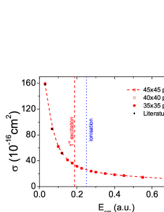
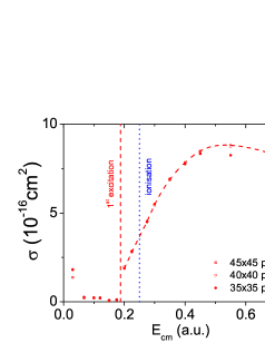
Figure 1: Calculated e+Ps(n=1) total (left panel) and inelastic (right panel) cross sections in a wide energy range. The dashed lines connecting calculated points is just drawn to guide an eye and does not represent complete calculation. Current calculations are well converged, which becomes clear by increasing employed Lagrange-mesh basis size. Below Ps(n=2) excitation threshold calculated total cross sections are compared with ones compiled from the literature [15, 17] and represented by full black squares.

In figure 1 electron scattering on the ground state of positronium (Ps(n=1)) atom cross section are presented. Calculation have been realized in a broad energy region, starting with a purely elastic case and spreading well above the positronium ionization threshold. Below the positronium excitation threshold results of this work are compared with the most accurate values from literature, summarized in Table.I of ref. [17].

Present calculations have been performed by considering free e+Ps(n=1) waves to represent the incoming wave function in eq. (7-8). The inhomogeneous term arising from the incoming wave has been screened in eq. (11) for e+Ps(n=1) separations beyond $y_{e}ps=35$ a.u. Partial wave expansion has been limited to max$(l_{x},l_{y})\leq 9$ and proved to be sufficient to get well converged results, calculations were also limited to total angular momentum $L\leq$5.

As can be seen in figure 1 a basis of 35 Lagrange-Laguerre mesh functions in $x$ and $y$ direction is enough to get converged results in a broad energy region. Only well beyond positronium ionization threshold a basis 35x35 functions turns to be insufficient in describing inelastic cross section, nevertheless convergence is reached by increasing basis to 40x40 functions.

As discussed in our previous works employing complex scaling [21, 2], large complex scaling angles are not suited to perform scattering calculations in $A>2$ particle systems. This work reconfirmed this feat. In this work complex scaling parameter has been limited to $\theta<10^{\circ}$, with $\theta=7-8^{\circ}$ representing an optimal choice. Regardless simplicity of the employed approach calculations turn to be very accurate and are in line with most accurate published values. The phaseshifts calculated below the Ps(n=2) threshold differ from ones reported in [15, 17] by less than 0.5$\%$.

As it is well known, complex scaling operation breaks Hermiticity of the Hamiltonian. Consequently the unitarity of S-matrix is not provided by the symmetry properties of the CS equations. This is the reason why using complex scaling it is more difficult to attain numerically the unitarity of S-matrix than to get highly accurate phaseshifts. Regardless this fact the unitarity of S-matrix in presented e+Ps(n=1) calculations is assured with three-digit accuracy once electron impact energy exceeds 0.03 a.u. This is clearly demonstrated by analyzing inelastic e+Ps(n=1) cross section, extracted based on the unitarity property of the S-matrix. In particular, inelastic cross section is consistent with a zero value in the purely elastic region, below the Ps(n=2) threshold. Accurate description of the nearthreshold collisions is naturally the most problematic case for the complex-scaling method. After the complex scaling operation outgoing waves converge with an exponential factor -$krsin\theta$, where $k$ is a relative momenta of scattering clusters and $r$ is a target-projectile separation distance. This exponent vanishes for low impact energies and therefore approximation of the outgoing waves by using square-integrable basis functions becomes inefficient.

4.2 $e^{-}$+H scattering

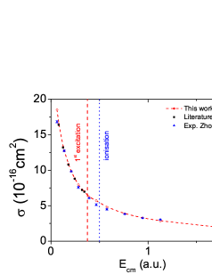
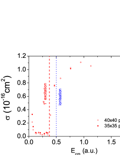
Figure 2: The same as in Fig. 1 but for $e^{-}$+H(n=1) scattering. Calculated values for the total cross section are compared with experimental data of Zhou et al. [22]. Below $H(n=2)$ excitation threshold calculated total cross sections are compared with ones compiled from the literature [23] and represented by full black squares.

In the figure 2 calculations of electron scattering on the ground sate of Hydrogen atom are presented. Present calculations have been performed using the same setup as for e=Ps(n=1) case, described in the last section. A free e+H(n=1) wave is considered when separating inhomogeneous term in eq. (7-8). 35-40 Lagrange-mesh functions were employed for discretizing radial dependence of FM amplitudes in $x$ and $y$ directions and proved to be enough to get converged results. Calculated values agree perfectly with ones found in literature [23] as well as with the experimental data of Zhou et al. [22]. Only the last point (at 1.87 a.u.) seems to underestimate experimental total cross section. Total cross section in this energy region, well above the Hydrogen ionization threshold, has non-negligible contribution of high angular momentum states (beyond $L$=5), which have not been included in a present calculation.

The phaseshifts calculated below the $H(n=2)$ threshold agree perfectly well with the most accurate calculations found in the literature. All the phaseshifts fall within the limits defined by the values compiled in reference [23].

As pointed out in the previous section, presenting the e+Ps(n=1) scattering, complex scaling technique turns to be the most difficult to apply at very low energies, close to the threshold. By reducing energy it turns increasingly difficult to preserve unitarity of the calculated S-matrix. This feat is best demonstrated by the deviation from the zero-value of the inelastic $e^{-}-H(n=1)$ cross section close to $H(n=1)$ threshold (see two lowest energy points, situated at $E_{c}m=0.0624$ and $0.08$ a.u. respectively). Naturally unitarity of the calculated S-matrix improves once number of basis functions is increased, nevertheless at very low energies this convergence turns to be rather slow.

4.3 $e^{+}$-H(n=1)$\leftrightarrows$p+Ps(n=1) scattering

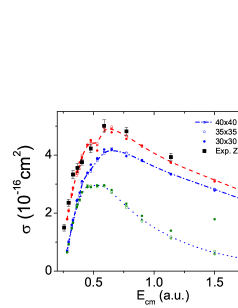
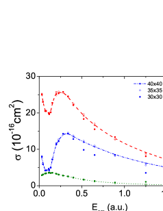
Figure 3: Study of e⁺+H(n=1) (left panel) and p+Ps(n=1) (right panel) collisions. Evolution. of total (red), total inelastic (blue) and $e^{+}$+H(n=1)$\leftrightarrows$ p+Ps(n=1) (olive) cross sections presented with energy. Three sets of calculations performed using different radial basis sizes. Calculated total cross section for a e⁺+H(n=1) process is compared with experimental data of Zhou et al. [22].

There is an increased interest in studying (anti)proton-positronium collisions in view of the possible production of antihydrogen atoms. This system was mostly explored using different variations of close-coupling method [24, 25]; There also exist calculations based on Hyperspherical-Harmonics [26],variational method [27, 28] as well as Faddeev-Merkuriev equations [10, 29] but these limited to the energy region of a few lowest energy excitations of either Hydrogen or Positronium atom.

Elastic $e^{+}$+H(n=1) collisions below positronium excitation threshold does not present any new features compared to $e^{-}$+H(n=1) or e+Ps(n=1) elastic scattering, discussed in two previous subsections. Therefore I will concentrate on the energy region above p+Ps(n=1) production threshold. In figure 3 calculations performed by considering only a free $e^{+}$+H(n=1) (left panel) or $p-Ps(n=1)$ (right panel) wave when separating inhomogeneous term in eq. (7-8).

Calculations considering $e^{+}$+H(n=1) entrance channel are well converged for a moderate basis of 30x30 Lagrange-mesh functions and does not depend on the variation of CS parameter in the range $\theta=5-10^{\circ}$. Results of Present calculations agree perfectly well with other theoretical calculations as well as with the experimental data of Zhou et al. [22]. Experimental total cross section becomes slightly larger only for the highest energy point calculated, which has still to non-negligible contribution of high angular momentum scattering not included in a present calculations. For this point contribution of $L$=7 state, the largest total angular momentum state considered in this calculation, still accounts for $\approx 10\%$ of total cross section, whereas this state has negligible contribution at lower energies. Unitarity of the S-matrix is well preserved, which is demonstrated by the feat that below H(n=2) excitation threshold inelastic cross section agrees with a Ps(n=1) production one (at these energies Ps(n=1) production represents the only inelastic channel).

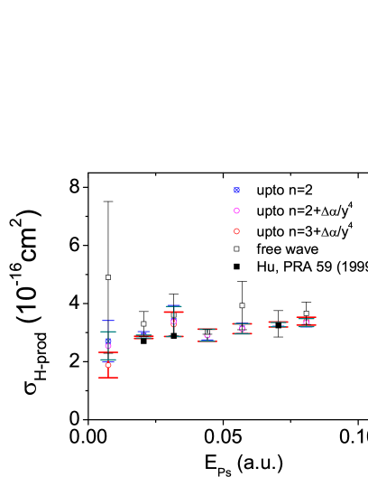
Figure 4: Calculation of the Hydrogen production cross section for p+Ps(n=1) collisions in the Ore gap region. Calculations using different assumptions for inhomogeneous term, based on distorted incoming wave of p+Ps(n=1), were performed. These results are compared with calculations of Hu [29], using conventional boundary condition method.

Calculations considering p+Ps(n=1) entrance channel turns to be less accurate. In particular, problematic are the calculations performed in the Ore gap region and dominated by relatively low proton(positronium) impact energies. In this region inelastic p+Ps(n=1) cross section, extracted using unitarity property of S-matrix, is visibly not converged and improves moderately when increasing Lagrange-mesh basis size. On the other hand, Hydrogen production cross sections calculated from the non-diagonal S-matrix element coupling $e^{+}$+H(n=1) and p+Ps(n=1) channels turns to be accurate and well converged even at very low energies.

Even though the low energy region is not the most relevant region to use complex scaling method – it is still worthy to pay more attention to the Ore gap region, where p+Ps(n=1) cross sections converge slowly. In order to improve convergence I have constructed inhomogeneous term in eq. (7,8) based on distorted waves instead of simple free waves used before. Effect of the choice of inhomogeneous term is studied in figure 4 by comparing inelastic p+Ps(n=1) cross sections in the problematic Ore gap region. These calculations were performed using a basis of 30x30 Lagrange-mesh functions, with CS parameter set to $\theta=5^{\circ}$ and total angular momentum expansion limited to $L$=3. Four types of distorted waves, based on the choice of long-range potential in eq. (9), have been used:

• distorted wave by considering long-range dipole coupling of Ps(n$\leq$2) states, with $\lambda_{ab}(y_{\alpha})=-C_{\alpha}\langle\varphi_{b,l_{x}^{(b)}}(\vec{x}_{\alpha})|\vec{x}_{\alpha}|\varphi_{a,l_{x}^{(a)}}(\vec{x}_{\alpha})\rangle/\tilde{y_{ab}}_{\alpha}^{2}$

• considering long-range dipole coupling of Ps(n$\leq$2) states together with a residual p+Ps(n=1) polarization potential

• dipole coupling of Ps(n$\leq$3) states together with a residual p+Ps(n=1) polarization potential

• inhomogeneous term based on free wave

In the figure 4 calculated p+Ps(n=1)$\leftrightarrows e^{+}$+H(n=1) reaction cross section is presented as a range, obtained by comparing three different values: cross sections calculated from non-diagonal S-matrix elements ($S_{e^{+}+H(n=1),p+Ps(n=1)}$ and $S_{p-Ps(n=1),e^{+}+H(n=1)}$) as well as cross section extracted from diagonal S-matrix element $S_{p-Ps(n=1),p-Ps(n=1)}$ via unitarity condition. One can see that by using distorted waves to construct inhomogeneous term one may considerably improve accuracy of the calculated cross sections even at very low energies. Inclusion of the dipole coupling of Ps(n$\leq$2) states is already enough to get rather accurate results, in agreement with ones from ref. [29], which were obtained by employing conventional boundary condition approach. By considering more complete asymptotic p+Ps(n=1) interaction to determine distorted incoming wave results improve further.

5 Conclusion

Coulombic three-body scattering problem have been addressed since the outset of Quantum Mechanics, however yet have not been fully resolved by mathematically rigorous methods. In this work it has been demonstrated that conventional smooth complex scaling method can be adapted to solve Coulombic three-body problems. A novel method has been developed, which combines complex scaling, distorted wave and Faddeev-Merkuriev equation formalisms. This formalism has been tested in studying three realistic Coulombic problems: electron scattering on ground states of Hydrogen and Positronium atoms as well as a $e^{+}$+H(n=1) $\leftrightarrows$ p+Ps(n=1) reaction.

Accurate results were obtained in a wide energy region, also extending beyond the atom ionization threshold. Calculations for high projectile impact energies turns to be very accurate and reliable. They agree perfectly with the available experimental data. On the other hand complex-scaling technique has natural deficiency in describing very low energy scattering. Still it is demonstrated that by using distorted incoming waves also description of the scattering process at very low energies can be significantly improved.

Next challenge is to consider charged particle scattering on the excited states of Hydrogen-type atoms. Additional complications should arise due to the presence of long range dipole coupling between the energy degenerate excited target states. It is not obvious if in such a system inhomogeneous term can be screened without visible complications as has been done for the scattering on ground state targets in this work. Distorted wave formalism might be very useful in achieving this goal.

On the other hand smooth complex scaling technique is easily adaptable by any numerical technique and might be easily incorporated to treat scattering problems in $N\geq 3$ systems. Worths noting, that this method has been already successfully adapted to describe the systems dominated by short-range interactions [2, 30]. Findings of this work brings optimism that Coulombic scattering may be finally addressed in the systems constituting four charged particles. The feat yet never addressed by the ab-initio techniques.

5.1 Acknowledgments*

This work was granted access to the HPC resources of TGCC and IDRIS under the allocation 2015-x2015056006 made by GENCI. We thank the staff members of the TGCC and IDRIS for their constant help.

References

-
[1]
V. I. Korobov, J. C. J. Koelemeij, L. Hilico, J.-P. Karr,
Theoretical
hyperfine structure of the molecular hydrogen ion at the 1 ppm level, Phys.
Rev. Lett. 116 (2016) 053003.
doi:10.1103/PhysRevLett.116.053003.
URL http://link.aps.org/doi/10.1103/PhysRevLett.116.053003 -
[2]
J. Carbonell, A. Deltuva, A. Fonseca, R. Lazauskas,
Bound
state techniques to solve the multiparticle scattering problem, Progress in
Particle and Nuclear Physics 74 (2014) 55 – 80.
doi:http://dx.doi.org/10.1016/j.ppnp.2013.10.003.
URL http://www.sciencedirect.com/science/article/pii/S0146641013000938 - [3] J. Nuttal, H. L. Cohen, Method of complex coordinates for three-body calculations above the breakup threshold, Phys. Rev. 188 (4) (1969) 1542–1544. doi:10.1103/PhysRev.188.1542.
-
[4]
B. Simon,
The
definition of molecular resonance curves by the method of exterior complex
scaling, Physics Letters A 71 (2) (1979) 211 – 214.
doi:http://dx.doi.org/10.1016/0375-9601(79)90165-8.
URL http://www.sciencedirect.com/science/article/pii/0375960179901658 -
[5]
P. L. Bartlett,
A complete
numerical approach to electron–hydrogen collisions, Journal of Physics B:
Atomic, Molecular and Optical Physics 39 (22) (2006) R379.
URL http://stacks.iop.org/0953-4075/39/i=22/a=R01 -
[6]
M. V. Volkov, E. A. Yarevsky, S. L. Yakovlev,
Potential splitting
approach to the three-body coulomb scattering problem, EPL (Europhysics
Letters) 110 (3) (2015) 30006.
URL http://stacks.iop.org/0295-5075/110/i=3/a=30006 - [7] L. D. Faddeev, Scattering theory for a three particle system, Sov. Phys. JETP 12 (1961) 1014–1019.
- [8] S. P. Merkuriev, Ann. Phys. (N.Y.) 130 (1980) 395.
- [9] M. Gailitis, R. Damburg, Sov. Phys. JETP 17 (1963) 1107.
-
[10]
C. Y. Hu, D. Caballero, Z. Papp,
Induced
long-range dipole-field-enhanced antihydrogen formation in the
reaction, Phys. Rev. Lett. 88 (2002) 063401.
doi:10.1103/PhysRevLett.88.063401.
URL http://link.aps.org/doi/10.1103/PhysRevLett.88.063401 -
[11]
T. Berggren,
On
resonance contributions to sum rules in nuclear physics, Physics Letters B
44 (1) (1973) 23 – 25.
doi:10.1016/0370-2693(73)90289-X.
URL http://www.sciencedirect.com/science/article/pii/037026937390289X - [12] B. Giraud, K. Kato, O. A., J. of Phys. A 37.
- [13] D. Baye, The lagrange-mesh method, Physics Reports 565 (2015) 1–107.
-
[14]
R. Lazauskas,
Scattering of
heavy charged particles in atomic and nuclear systems, Ph.D. thesis,
Université Joseph Fourier, Grenoble (October 2003).
URL http://tel.ccsd.cnrs.fr/documents/archives0/00/00/41/78/ - [15] S. J. Ward, J. W. Humberstonz, M. R. C. McDowell, J. Phys. B 20 (1987) 127.
-
[16]
C.-Y. Hu, A. A. Kvitsinsky,
Resonances in
-ps elastic scattering via a direct solution of
the three-body scattering problem, Phys. Rev. A 50 (1994) 1924–1926.
doi:10.1103/PhysRevA.50.1924.
URL http://link.aps.org/doi/10.1103/PhysRevA.50.1924 -
[17]
A. Igarashi, S. Nakazaki, A. Ohsaki,
Phase shifts of
scatterings and photodetachment cross sections of
, Phys. Rev. A 61 (2000) 032710.
doi:10.1103/PhysRevA.61.032710.
URL http://link.aps.org/doi/10.1103/PhysRevA.61.032710 -
[18]
A. Basu, A. S. Ghosh,
Doubly excited
resonant states of positronium negative ion, Phys. Rev. A 72 (2005) 062507.
doi:10.1103/PhysRevA.72.062507.
URL http://link.aps.org/doi/10.1103/PhysRevA.72.062507 -
[19]
Y. Zhou, S. Watanabe, O. I. Tolstikhin, T. Morishita,
Hyperspherical
calculations of ultralow-energy collisions in coulomb three-body systems,
Phys. Rev. A 92 (2015) 032713.
doi:10.1103/PhysRevA.92.032713.
URL http://link.aps.org/doi/10.1103/PhysRevA.92.032713 -
[20]
S. Gilmore, J. E. Blackwood, H. Walters,
Electron/positron
collisions with positronium, Nuclear Instruments and Methods in Physics
Research Section B: Beam Interactions with Materials and Atoms 221 (2004) 124
– 128, proceedings of the {XII} International Workshop on Positron and
Positronium Physics.
doi:http://dx.doi.org/10.1016/j.nimb.2004.03.042.
URL http://www.sciencedirect.com/science/article/pii/S0168583X04003787 -
[21]
R. Lazauskas, J. Carbonell,