The production rate of the system-bath mutual information

Abstract

When an open system is contacted with several thermal baths, the entropy produced by the irreversible processes ($dS_{\mathrm{i}}=dS-\sum_{\alpha}\text{\dj}Q_{\alpha}/T_{\alpha}$) keeps increasing, and this entropy production rate is always non-negative. But when the system is contacted with some non-thermal baths containing quantum coherence or squeezing, this entropy production formula does not apply. In this paper, we study the increasing rate of the mutual information between the open system and its environment. When the baths are canonical thermal ones, we prove that this mutual information production rate could exactly return to the previous entropy production rate. Further, we study an example of a single boson mode contacted with multiple squeezed thermal baths, where the conventional entropy production rate does not apply, and we find that this mutual information production rate still keeps non-negative, which means the monotonic increasing of the correlation between the system and its environment.

I Introduction

The entropy change of a system can be considered to come from two origins, i.e., $dS=dS_{\mathrm{e}}+dS_{\mathrm{i}}$ De Groot and Mazur (1962); Nicolis and Prigogine (1977); Reichl (2009); Kondepudi and Prigogine (2014), where $dS_{\mathrm{e}}$ comes from the exchange with external sources, and it could be either positive or negative; $dS_{\mathrm{i}}$ is the entropy change due to the irreversible processes. Then the 2nd law is simply stated as $dS_{\mathrm{i}}/dt\geq 0$, which means the entropy produced by the irreversible processes always increases, and $R_{\mathrm{ep}}:=dS_{\mathrm{i}}/dt$ is called the entropy production rate (EPr).

When the system is contacted with a thermal bath with temperature $T$, we have $dS_{\mathrm{e}}=\text{\text{\dj}}Q/T$ (hereafter we refer it as the thermal entropy), where $\text{\dj}Q$ is the heat flowing into the system. If we have multiple independent thermal baths with different temperatures $T_{\alpha}$ (Fig. 1), the EPr becomes

$$\frac{dS_{\mathrm{i}}}{dt}=\frac{dS}{dt}-\sum_{\alpha}\frac{1}{T_{\alpha}}\frac{dQ_{\alpha}}{dt}:=R_{\mathrm{ep}},$$ (1)

where $\text{\dj}Q_{\alpha}$ is the heat coming from bath-$\alpha$ De Groot and Mazur (1962); Kondepudi and Prigogine (2014).

Further, when an open quantum system is weakly coupled with the multiple thermal baths, usually its dynamics can be described by the following Lindblad (GKSL) equation Gorini et al. (1976); Lindblad (1976),

$$\dot{\rho}=i[\rho,\hat{H}_{S}]+\sum_{\alpha}{\cal L}_{\alpha}[\rho].$$ (2)

where ${\cal L}_{\alpha}[\rho]$ describes the dissipation due to bath-$\alpha$. Utilizing $\dot{S}[\rho]=-\mathrm{tr}[\dot{\rho}\ln\rho]$ and $\dot{Q}_{\alpha}=\mathrm{tr}\big{[}\hat{H}_{S}\cdot{\cal L}_{\alpha}[\rho]\big{]}$, the EPr (1) can be rewritten as the following Spohn formula (denoted as $R_{\mathrm{Sp}}$ hereafter) Spohn (1978); Spohn and Lebowitz (1978); Alicki (1979); Boukobza and Tannor (2007); Kosloff (2013); *kosloff_quantum_2016; Cai et al. (2014)

$$R_{\mathrm{ep}}=\sum_{\alpha}\mathrm{tr}\big{[}(\ln\rho_{\mathrm{ss}}^{(\alpha)}-\ln\rho)\cdot{\cal L}_{\alpha}[\rho]\big{]}:=R_{\mathrm{Sp}}.$$ (3)

Here we call $\rho_{\mathrm{ss}}^{(\alpha)}=Z_{\alpha}^{-1}\exp[-\hat{H}_{S}/T_{\alpha}]$ the partial steady state associated with bath-$\alpha$, satisfying ${\cal L}_{\alpha}[\rho_{\mathrm{ss}}^{(\alpha)}]=0$. It can be proved that $R_{\mathrm{Sp}}\geq 0$, which means the irreversible entropy production keeps increasing (see the proof in Appendix A or Ref. Spohn (1978); Spohn and Lebowitz (1978)).

However, in the above discussion, the thermal entropy $dS_{\mathrm{e}}=\text{\dj}Q/T$ only applies for canonical thermal baths. If the bath is some non-canonical state containing quantum coherence or squeezing Scully et al. (2003); Roßnagel et al. (2014); Manzano et al. (2016), the temperature is not well defined, thus it is no more proper to use $\text{\dj}Q/T$ for $dS_{\mathrm{e}}$ Gardas and Deffner (2015), and the relations $R_{\mathrm{ep}}=R_{\mathrm{Sp}}$ or $R_{\mathrm{ep}}\geq 0$ no longer hold either.

Therefore, for such non-thermal baths, the conventional thermodynamic description of the EPr does not apply. And it is believed that corrections of some work Quan et al. (2005, 2006); Gelbwaser-Klimovsky and Kurizki (2014), or excess heat Gardas and Deffner (2015) should be considered in these baths.

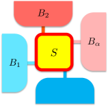
Figure 1: (Color online) Demonstration for an open quantum system ($S$) interacting with its environment composed of multiple baths ($B_{\alpha}$). The baths are independent from each other, and do not have to be canonical thermal states.

Here we replace the thermal entropy term $-\dot{Q}_{\alpha}/T_{\alpha}$ by the von Neumann entropy of bath-$\alpha$, $\dot{S}_{B\alpha}=-\mathrm{tr}[\dot{\rho}_{B\alpha}\ln\rho_{B\alpha}]$. Further, we assume the multiple baths are independent from each other, thus it leads to $\sum_{\alpha}\dot{S}_{B\alpha}=\dot{S}_{B}$. Then this generalization becomes

$$R_{{\cal I}}=\frac{dS_{S}}{dt}+\frac{dS_{B}}{dt}=\frac{d}{dt}(S_{S}+S_{B}-S_{SB})=\frac{d}{dt}{\cal I}_{SB}.$$ (4)

Here $\dot{S}_{SB}=0$ since the total system $S+B$ evolves unitarily , and ${\cal I}_{SB}:=S_{S}+S_{B}-S_{SB}$ is just the mutual information between the system and its environment, which measures their correlation Nielsen and Chuang (2000); Esposito et al. (2010); Pucci et al. (2013); Parrondo et al. (2015); Alipour et al. (2016); Strasberg et al. (2017). Therefore, we call $R_{{\cal I}}$ the mutual information production rate (MIPr).

$R_{{\cal I}}$ has a clear physical meaning: a positive $R_{{\cal I}}$ indicates the correlation between the system and its environment is increasing. In the following, we are going to show that, indeed this MIPr (4) has a quite close connection with the previous EPr (1). When the bath of the open system are thermal ones, we can prove that this MIPr could exactly return to the conventional thermodynamic description of the EPr in the weak coupling limit, namely, $R_{{\cal I}}=R_{\mathrm{ep}}$. That means, for thermal bath, the conventional entropy production can be equivalently interpreted as the mutual information production, and the 2nd law statement $(R_{{\cal I}}=)R_{\mathrm{ep}}\geq 0$ can be also understood as the system-bath correlation always keeps increasing.

Further, we will study an example of a single boson contacted with multiple squeezed thermal baths. In this case, the conventional EPr does not apply. We calculate the MIPr under the weak coupling limit and Markovian approximation, and we find that it exactly equals to the Spohn formula for non-thermal baths, thus we can prove $R_{{\cal I}}\geq 0$, which means the monotonic increasing of the system-bath correlation also holds in this squeezed bath example.

II Mutual information production in thermal baths

Now we first consider the system is coupled with several thermal baths. In this case, the initial state of bath-$\alpha$ is $\rho_{B\alpha}(0)={\cal Z}_{\alpha}^{-1}\exp[-\hat{H}_{B\alpha}/T_{\alpha}]$. Assuming $\rho_{B\alpha}(t)$ does not change too much during evolution Breuer and Petruccione (2002); Scully and Zubairy (1997); Li et al. (2016), we have $\ln\rho_{B\alpha}(t)=\ln[\rho_{B\alpha}(0)+\delta\rho_{t}]\simeq\ln[\rho_{B\alpha}(0)]+o(\delta\rho_{t})$, thus the entropy change of bath-$\alpha$ is

$$\dot{S}_{B\alpha} =-\mathrm{tr}[\dot{\rho}_{B\alpha}(t)\ln\rho_{B\alpha}(t)]\simeq-\mathrm{tr}[\dot{\rho}_{B\alpha}(t)\cdot\ln\frac{e^{-\frac{\hat{H}_{B\alpha}}{T_{\alpha}}}}{{\cal Z}_{\alpha}}]$$

$$=\frac{1}{T_{\alpha}}\frac{d}{dt}\langle\hat{H}_{B\alpha}\rangle\simeq-\frac{\dot{Q}_{\alpha}}{T_{\alpha}}.$$ (5)

Here $-\frac{d}{dt}\langle\hat{H}_{B\alpha}\rangle$ is the energy loss of bath-$\alpha$, while $\dot{Q}_{\alpha}$ is the energy gain of the system from bath-$\alpha$, and they equal to each other in weak coupling limit. Assuming the baths are independent from each other, $\rho_{B}(t)\simeq\prod_{\alpha}\rho_{B\alpha}(t)$, the MIPr becomes

$$R_{{\cal I}}=\dot{S}_{S}+\sum_{\alpha}\dot{S}_{B\alpha}=\dot{S}_{S}-\sum_{\alpha}\frac{\dot{Q}_{\alpha}}{T_{\alpha}}=R_{\mathrm{ep}}.$$ (6)

Therefore, for thermal baths, the MIPr (4) equals to the conventional thermodynamic description of the EPr (1).

Thus, the 2nd law statement $R_{\mathrm{ep}}\geq 0$ is equivalent as $R_{{\cal I}}\geq 0$, which means the mutual information between the system and its environment keeps increasing monotonically. This can be understood as an equivalent statement for the entropy production when the baths are canonical thermal ones. We notice that this equivalence was also shown in the “correlation entropy” approach Esposito et al. (2010); Pucci et al. (2013); Strasberg et al. (2017).

III Mutual information production in Squeezed baths

Now we study an example of a single boson mode interacting with multiple squeezed thermal baths Roßnagel et al. (2014); Manzano et al. (2016); Kosloff and Rezek (2016). In this case, the thermal entropy $dS_{\mathrm{e}}=\text{\dj}Q/T$ cannot be used, and neither does the EPr (1). Here we calculate the MIPr (4), and we will prove it just equals to the Spohn formula for non-thermal baths, and thus could still keep non-negative, $R_{{\cal I}}\geq 0$.

III.1 Master equation and Spohn formula

The Hamiltonian of the single boson mode and the bosonic bath are $\hat{H}_{S}=\Omega\,\hat{a}^{\dagger}\hat{a}$, $\hat{H}_{B}=\sum_{\alpha}\hat{H}_{B\alpha}$ and $\hat{H}_{B\alpha}=\sum_{k}\omega_{\alpha k}\,\hat{b}_{\alpha k}^{\dagger}\hat{b}_{\alpha k}$, and they interact through $\hat{V}_{SB}=\sum_{\alpha}\hat{a}^{\dagger}\hat{B}_{\alpha}+\hat{a}\hat{B}_{\alpha}^{\dagger}$. Here $\hat{B}_{\alpha}=\sum g_{\alpha k}\hat{b}_{\alpha k}$ is the operator of bath-$\alpha$, and the initial states of the baths are squeezed thermal ones (hereafter all the density matrices are written in the interaction picture),

$$\rho_{B\alpha}^{0}=\frac{1}{{\cal Z}_{\alpha}}e^{-\beta_{\alpha}\,{\cal S}_{\alpha}\hat{H}_{B\alpha}{\cal S}_{\alpha}^{\dagger}},\quad\beta_{\alpha}:=T_{\alpha}^{-1},$$ (7)

$${\cal S}_{\alpha}:=\prod_{k}\exp[\frac{1}{2}\lambda_{\alpha k}^{*}\hat{b}_{\alpha k}^{2}-\mathbf{h.c.}],\quad\lambda_{\alpha k}=r_{\alpha k}e^{-i\theta_{\alpha k}}.$$

Here ${\cal S}_{\alpha}$ is the squeezing operator for the boson modes in bath-$\alpha$. With Born-Markovian approximation, we obtain a master equation $\dot{\rho}=\sum_{\alpha}{\cal L}_{\alpha}[\rho]$ for the open system alone Breuer and Petruccione (2002); Walls and Milburn (2008), where

$${\cal L}_{\alpha}[\rho] =\frac{\gamma_{\alpha}}{2}\Big{[}\tilde{\mathfrak{n}}_{\alpha}\big{(}2\hat{a}^{\dagger}\rho\hat{a}-\{\hat{a}\hat{a}^{\dagger},\rho\}\big{)}+(\tilde{\mathfrak{n}}_{\alpha}+1)\big{(}2\hat{a}\rho\hat{a}^{\dagger}-\{\hat{a}^{\dagger}\hat{a},\rho\}\big{)}$$

$$-\tilde{\mathfrak{u}}_{\alpha}\big{(}2\hat{a}^{\dagger}\rho\hat{a}^{\dagger}-\{(\hat{a}^{\dagger})^{2},\rho\}\big{)}-\tilde{\mathfrak{u}}_{\alpha}^{*}\big{(}2\hat{a}\rho\hat{a}-\{\hat{a}^{2},\rho\}\big{)}\Big{]}.$$

The coupling spectrums of the squeezed bath-$\alpha$ are $J_{\alpha}(\omega):=2\pi\sum_{k}|g_{\alpha k}|^{2}\delta(\omega-\omega_{\alpha k})$ and $K_{\alpha}(\omega):=2\pi\sum_{k}g_{\alpha k}^{2}\delta(\omega-\omega_{\alpha k})$. Without loss of generality, we omit the phase of $g_{\alpha k}$ and thus $K_{\alpha}(\omega)=K_{\alpha}^{*}(\omega)=J_{\alpha}(\omega)$. Here we denote $\gamma_{\alpha}:=J_{\alpha}(\Omega)=K_{\alpha}(\Omega)$, and the parameters $\tilde{\mathfrak{n}}_{\alpha}:=\tilde{\mathsf{n}}_{\alpha}(\Omega)$, $\tilde{\mathfrak{u}}_{\alpha}:=\tilde{\mathsf{u}}_{\alpha}(\Omega)$ are calculated from $\tilde{\mathsf{n}}_{\alpha}(\omega_{k}):=\mathrm{tr}[\rho_{B\alpha}^{0}\hat{b}_{\alpha k}^{\dagger}\hat{b}_{\alpha k}]$, $\tilde{\mathsf{u}}_{\alpha}(\omega_{k}):=-\mathrm{tr}[\rho_{B\alpha}^{0}\hat{b}_{\alpha k}^{2}]$ (see Appendix B). The master equation gives

$$\frac{d}{dt}\langle\tilde{a}(t)\rangle=-\sum_{\alpha}\frac{\gamma_{\alpha}}{2}\langle\tilde{a}\rangle,\quad\frac{d}{dt}\langle\tilde{a}^{2}\rangle=-\sum_{\alpha}\gamma_{\alpha}[\langle\tilde{a}^{2}\rangle-\tilde{\mathfrak{u}}_{\alpha}],$$

$$\frac{d}{dt}\langle\tilde{a}^{\dagger}\tilde{a}\rangle=-\sum_{\alpha}\gamma_{\alpha}[\langle\tilde{n}_{a}\rangle-\tilde{\mathfrak{n}}_{\alpha}].$$ (8)

Here we denote $\hat{n}_{a}:=\hat{a}^{\dagger}\hat{a}$, and $\langle\tilde{o}(t)\rangle:=\mathrm{tr}[\rho\hat{o}(t)]$ gives variables in the rotating frame .

The partial steady states $\rho_{\mathrm{ss}}^{(\alpha)}$, which satisfies ${\cal L}_{\alpha}[\rho_{\mathrm{ss}}^{(\alpha)}]=0$, are now squeezed thermal states,

$$\rho_{\mathrm{ss}}^{(\alpha)}=\frac{1}{Z_{\alpha}}\exp[-\beta_{\alpha}\Omega\cdot\mathsf{S}_{\alpha}\hat{a}^{\dagger}\hat{a}\mathsf{S}_{\alpha}^{\dagger}],$$ (9)

$$\mathsf{S}_{\alpha}:=\exp[-(\frac{1}{2}\zeta_{\alpha}^{*}\hat{a}^{2}-\mathbf{h.c.})],\>\zeta_{\alpha}=\lambda_{\alpha k}\big{|}_{\omega_{k}=\Omega}:=r_{\alpha}e^{i\theta_{\alpha}}.$$

Here $\mathsf{S}_{\alpha}$ is a squeezing operator for the system. Although the baths are not thermal ones, we can still write down the Spohn formula $R_{\mathrm{Sp}}=\sum_{\alpha}R_{\mathrm{Sp}}^{(\alpha)}$, where

$$R_{\mathrm{Sp}}^{(\alpha)} :=\mathrm{tr}\big{[}(\ln\rho_{\mathrm{ss}}^{(\alpha)}-\ln\rho)\cdot{\cal L}_{\alpha}[\rho]\big{]}$$

$$:=\chi_{\alpha}-\mathrm{tr}\big{[}\ln\rho\cdot{\cal L}_{\alpha}[\rho]\big{]}$$ (10)

and we can prove $R_{\mathrm{Sp}}^{(\alpha)}\geq 0$ and $R_{\mathrm{Sp}}\geq 0$ hold also in this non-thermal case (Appendix A).

However, since the above Spohn formula $R_{\mathrm{Sp}}$ for non-thermal baths no more comes from the thermodynamic EPr (1), thus its physical meaning is unclear now. In the thermal case, the 1st term in $R_{\mathrm{Sp}}^{(\alpha)}$, $\chi_{\alpha}:=\mathrm{tr}\big{[}\ln\rho_{\mathrm{ss}}^{(\alpha)}\cdot{\cal L}_{\alpha}[\rho]\big{]}$, gives the changing rate of the thermal entropy ($\chi_{\alpha}=-\dot{Q}_{\alpha}/T_{\alpha}$). But for the squeezed case, it becomes

$$\chi_{\alpha}=\frac{\Omega}{T_{\alpha}}\cdot\gamma_{\alpha}\Big{(}\cosh 2r_{\alpha}\cdot[\langle\tilde{n}_{a}(t)\rangle-\tilde{\mathfrak{n}}_{\alpha}]\\ -\frac{1}{2}\sinh 2r_{\alpha}[e^{-i\theta_{\alpha}}(\langle\tilde{a}^{2}(t)\rangle-\tilde{\mathfrak{u}}_{\alpha})+\mathbf{h.c.}]\Big{)}.$$ (11)

It is difficult to tell the physical meaning of this quantity. In the following, we will show that indeed Eq. (11) is just the changing rate of the von Neumann entropy of bath-$\alpha$, i.e., $\chi_{\alpha}=\dot{S}_{B\alpha}$, and then Eq. (10) directly leads to

$$R_{\mathrm{Sp}}=\sum_{\alpha}R_{\mathrm{Sp}}^{(\alpha)}=\dot{S}_{S}+\sum_{\alpha}\dot{S}_{B\alpha}=R_{{\cal I}}.$$ (12)

III.2 Bath entropy dynamics

Now we are going to calculate the entropy changing rate $\dot{S}_{B\alpha}$ of bath-$\alpha$ directly. To do this, we adopt the same trick as the thermal case. Assuming the squeezed baths do not change too much (interaction picture), the entropy of the bath evolves as

$$\frac{d}{dt}S[\rho_{B\alpha}(t)]\simeq- \mathrm{tr}[\dot{\rho}_{B\alpha}(t)\cdot\ln\frac{\exp[-\beta_{\alpha}\,{\cal S}_{\alpha}\hat{H}_{B\alpha}{\cal S}_{\alpha}^{\dagger}]}{{\cal Z}_{\alpha}}]$$

$$=\frac{d}{dt}\sum_{k}\frac{\omega_{\alpha k}}{T_{\alpha}}\Big{(} \cosh 2r_{\alpha k}\langle\tilde{b}_{\alpha k}^{\dagger}(t)\tilde{b}_{\alpha k}(t)\rangle$$

$$+\frac{1}{2}\sinh 2r_{\alpha k}[\langle\tilde{b}_{\alpha k}^{2}(t)\rangle e^{-i\theta_{\alpha k}}+\mathbf{h.c.}]\Big{)}.$$ (13)

Thus, the calculation of the bath entropy is now reduced as calculating the time derivative of the expectations of the bath operators like $\langle\tilde{b}_{\alpha k}^{\dagger}(t)\tilde{b}_{\alpha k}(t)\rangle$ and $\langle\tilde{b}_{\alpha k}^{2}(t)\rangle$.

This can be done with the help of the Heisenberg equations, $\dot{\hat{b}}_{\alpha k}=-i\omega_{\alpha k}\hat{b}_{\alpha k}-ig_{\alpha k}^{*}\hat{a}$, and $\dot{\hat{a}}=-i\Omega\hat{a}-i\sum_{\alpha}g_{\alpha k}\hat{b}_{\alpha k}$, which lead to the quantum Langevin equation Gardiner and Zoller (2004); Walls and Milburn (2008); Li et al. (2014)

$$\frac{d}{dt}\hat{a}=-i\Omega\hat{a}-\frac{1}{2}\Gamma\hat{a}-\hat{{\cal E}}(t).$$ (14)

Here $\Gamma:=\sum_{\alpha}\gamma_{\alpha}$ is the total decay rate, and $\gamma_{\alpha}$ are the same as those in the master equation; $\hat{{\cal E}}(t):=\sum_{\alpha}\hat{\xi}_{\alpha}(t)$ is the random force, and $\hat{\xi}_{\alpha}(t):=i\sum_{k}g_{\alpha k}\hat{b}_{\alpha k}(0)e^{-i\omega_{\alpha k}t}$ is the contribution from bath-$\alpha$. Thus $\hat{a}(t)$ and $\hat{b}_{\alpha k}(t)$ evolve as

$$\hat{a}(t)=\hat{a}(0)e^{-i\Omega t-\frac{\Gamma}{2}t}-\int_{0}^{t}ds\,e^{-i\Omega(t-s)-\frac{\Gamma}{2}(t-s)}\hat{{\cal E}}(s),$$ (15)

$$\hat{b}_{\alpha k}(t)=\hat{b}_{\alpha k}(0)e^{-i\omega_{\alpha k}t}-ig_{\alpha k}^{*}\int_{0}^{t}ds\,e^{-i\omega_{\alpha k}(t-s)}\hat{a}(s).$$

To further calculate the bath entropy change, now we are going to show the following two relations hold in the weak coupling limit and Markovian approximation:

$$\frac{d}{dt}\sum_{k}\mathfrak{f}_{k}\langle\tilde{b}_{\alpha k}^{\dagger}\tilde{b}_{\alpha k}\rangle \simeq\mathfrak{f}(\Omega)\cdot\gamma_{\alpha}[\langle\tilde{n}_{a}\rangle-\tilde{\mathfrak{n}}_{\alpha}],$$ (16)

$$\frac{d}{dt}\sum_{k}\mathfrak{h}_{k}\langle\tilde{b}_{\alpha k}^{2}\rangle+\mathbf{h.c.} \simeq-\mathfrak{h}(\Omega)\cdot\gamma_{\alpha}[\langle\tilde{a}^{2}\rangle-\tilde{\mathfrak{u}}_{\alpha}]+\mathbf{h.c.},$$

where $\mathfrak{f}_{k}$ and $\mathfrak{h}_{k}$ are arbitrary coefficients depending on $k$.

If we set $\mathfrak{f}_{k}=\frac{\omega_{\alpha k}}{T_{\alpha}}\cosh 2r_{\alpha k}$, $\mathfrak{h}_{k}=\frac{\omega_{\alpha k}}{2T_{\alpha}}\sinh 2r_{\alpha k}e^{-i\theta_{\alpha k}}$, and sum up the above two equations, then the left side simply gives $\dot{S}_{B\alpha}$ [Eq. (13)]; At the same time, the right side is just equal to $\chi_{\alpha}$ [Eq. (11)]. Thus we can prove $\chi_{\alpha}=\dot{S}_{B\alpha}$, namely, the term $\chi_{\alpha}=\mathrm{tr}\big{[}\ln\rho_{\mathrm{ss}}^{(\alpha)}\cdot{\cal L}_{\alpha}[\rho]\big{]}$ in the Spohn formula is just the changing rate of the von Neumann entropy of bath-$\alpha$.

Besides, if we set $\mathfrak{f}_{k}=\omega_{\alpha k}$ and $\mathfrak{h}_{k}=0$, the above relations lead to $\frac{d}{dt}\langle\hat{H}_{B\alpha}\rangle=\Omega\cdot\gamma_{\alpha}[\langle\tilde{n}_{a}\rangle-\tilde{\mathfrak{n}}_{\alpha}]=-\dot{Q}_{\alpha}$, which means the energy loss of bath-$\alpha$ is equal to the energy gain of the system from bath-$\alpha$ [as we utilized in the discussion below Eq. (5)].

The calculation of Eq. (16) goes as follows

$$\frac{d}{dt}\sum_{k}\mathfrak{f}_{k}\langle\tilde{b}_{\alpha k}^{\dagger}\tilde{b}_{\alpha k}\rangle=\sum_{k}\mathfrak{f}_{k}\cdot ig_{\alpha k}\langle\hat{a}^{\dagger}\hat{b}_{\alpha k}\rangle+\mathbf{h.c.}$$

$$= \sum_{k}\mathfrak{f}_{k}\cdot\Big{[}ig_{\alpha k}\langle\hat{a}^{\dagger}(t)\hat{b}_{\alpha k}(0)\rangle e^{-i\omega_{\alpha k}t}$$

$$+|g_{\alpha k}|^{2}\int_{0}^{t}ds\,e^{-i\omega_{\alpha k}(t-s)}\langle\hat{a}^{\dagger}(t)\hat{a}(s)\rangle\Big{]}+\mathbf{h.c.}$$ (17)

The 1st term in the bracket can be further calculated by substituting $\hat{a}(t)$ [Eq. (15)],

$$\sum_{k}\mathfrak{f}_{k}\cdot ig_{\alpha k}\langle\hat{a}^{\dagger}(t)\hat{b}_{\alpha k}(0)\rangle e^{-i\omega_{\alpha k}t}+\mathbf{h.c.}$$ (18)

$$= -\sum_{k}\mathfrak{f}_{k}|g_{\alpha k}|^{2}\int_{0}^{t}ds\,e^{[i(\Omega-\omega_{k})-\frac{\Gamma}{2}](t-s)}\langle\hat{b}_{\alpha k}^{\dagger}(0)\hat{b}_{\alpha k}(0)\rangle+\mathbf{h.c.}$$

$$= -\int_{0}^{t}ds\big{[}\int_{0}^{\infty}\frac{d\omega}{2\pi}e^{[i(\Omega-\omega)-\frac{\Gamma}{2}](t-s)}J_{\alpha}(\omega)\mathfrak{f}(\omega)\tilde{\mathsf{n}}_{\alpha}(\omega)\big{]}+\mathbf{h.c.}$$

Assuming the frequency integral in the bracket gives a fast-decaying function of $(t-s)$, we extend the time integral to $t\rightarrow\infty$ (Markovian approximation), and that gives

$$-\int_{0}^{\infty}\frac{d\omega}{2\pi}[\int_{0}^{\infty}ds\,e^{i(\Omega-\omega)s-\frac{1}{2}\Gamma s}]J_{\alpha}(\omega)\mathfrak{f}(\omega)\tilde{\mathsf{n}}_{\alpha}(\omega)+\mathbf{h.c.}$$

$$= -\int_{0}^{\infty}\frac{d\omega}{2\pi}\,J_{\alpha}(\omega)\mathfrak{f}(\omega)\tilde{\mathsf{n}}_{\alpha}(\omega)\cdot\frac{\Gamma}{(\frac{\Gamma}{2})^{2}+(\omega-\Omega)^{2}}$$

$$\simeq -\mathfrak{f}(\Omega)\cdot\gamma_{\alpha}\tilde{\mathfrak{n}}_{\alpha}.$$ (19)

The last line holds in the weak coupling limit $\Gamma\ll\Omega$ because the Lorentzian function in the integral approaches $2\pi\delta(\omega-\Omega)$.

To calculate the 2nd term of Eq. (17), we should notice $\langle\hat{a}^{\dagger}(t)\hat{a}(s)\rangle=\langle\tilde{a}^{\dagger}(s)\tilde{a}(s)\rangle e^{(i\Omega-\frac{\Gamma}{2})(t-s)}$ holds for $t\geq s$ (quantum regression theorem Breuer and Petruccione (2002); Gardiner and Zoller (2004)). Here $\langle\tilde{o}_{1}(t)\tilde{o}_{2}(s)\rangle$ is a correlation function in the rotating frame, defined by $\langle\tilde{o}_{1}(t)\tilde{o}_{2}(s)\rangle=\mathrm{tr}[\hat{o}_{1}\,{\cal E}_{t-s}\hat{o}_{2}\,{\cal E}_{s}\rho(0)]$ for $t\geq s$ Breuer and Petruccione (2002), where $\hat{o}_{1,2}$ are operators in Schrödinger picture, and ${\cal E}_{t}$ is the evolution operator solved from the above master equation in interaction picture, and $\rho(t)={\cal E}_{t-s}\rho(s)$. Similarly, $\langle\hat{o}_{1}(t)\hat{o}_{2}(s)\rangle$ are correlation functions in the non-rotating frame. Thus the 2nd term of Eq. (17) gives

$$\sum_{k}\mathfrak{f}_{k}\cdot|g_{\alpha k}|^{2}\int_{0}^{t}ds\,e^{-i\omega_{\alpha k}(t-s)}\langle\hat{a}^{\dagger}(t)\hat{a}(s)\rangle+\mathbf{h.c.}$$

$$\simeq \int_{0}^{\infty}\frac{d\omega}{2\pi}\,\mathfrak{f}(\omega)J_{\alpha}(\omega)\cdot\langle\tilde{n}_{a}(t)\rangle\int_{0}^{\infty}ds\,e^{i(\Omega-\omega)s-\frac{\Gamma}{2}s}+\mathbf{h.c.}$$

$$= \langle\tilde{n}_{a}(t)\rangle\cdot\int_{0}^{\infty}\frac{d\omega}{2\pi}\,\mathfrak{f}(\omega)J_{\alpha}(\omega)\cdot\frac{\Gamma}{(\frac{\Gamma}{2})^{2}+(\omega-\Omega)^{2}}$$

$$\simeq \gamma_{\alpha}\cdot\mathfrak{f}(\Omega)\langle\tilde{n}_{a}(t)\rangle.$$ (20)

Again we adopted the Markovian approximations as before, and $\langle\tilde{n}_{a}(s)\rangle$ is taken out of the integral directly.

Therefore, summing up Eqs. (19, 20), we obtain the 1st relation in Eq. (16). The 2nd relation can be obtained through the similar way (see Appendix B). Then, by setting proper coefficients $\mathfrak{f}_{k}$ and $\mathfrak{h}_{k}$ in Eq. (16), we can prove $\chi_{\alpha}=\dot{S}_{B\alpha}$, and further $R_{{\cal I}}=R_{\mathrm{Sp}}$. Since we can prove the Spohn formula $R_{\mathrm{Sp}}\geq 0$, the MIPr $R_{{\cal I}}$ also keeps positive, which means the the system-bath mutual information, or their correlation, still keeps increasing monotonically in this non-thermal case.

IV Summary

In this paper, we study the production of the mutual information between the system and its environment. We find that this MIPr (4) has a close connection with the conventional thermodynamic description of the EPr (1): when the baths of the open system are canonical thermal ones, this MIPr could exactly return to the previous EPr. Therefore, the 2nd law statement $R_{\mathrm{ep}}\geq 0$ can be equivalently understood as saying the system-bath correlation always keeps increasing.

Besides, we also study an example of a single boson mode contacted with multiple squeezed thermal baths. In this case, the temperatures of the baths are not well defined and the previous EPr does not apply. We proved that the MIPr is still positive, which means the monotonic increasing of the system-bath correlation also exists in this case. Definitely it is worthful to study the MIPr in more non-thermal systems.

We remark that the proof for the positivity of the MIPr and the Spohn formula relies on the fact the dynamics of the system can be well described by a Markovian master equation with the Lindblad (GKSL) form. If this is not fulfilled Pucci et al. (2013); Sharma and Rabani (2015); Li et al. (2016); Lampo et al. (2016), the positivity cannot be guaranteed.

Our study indicates it is the system-bath correlation that keeps increasing monotonically although the total $S+B$ system evolves unitarily. This idea is also consistent with some other fundamental studies on thermodynamics, such as the local relaxation hypothesis Cramer et al. (2008); *eisert_quantum_2015, the entanglement based thermodynamics Popescu et al. (2006); *goldstein_canonical_2006, and the mutual information understanding of the Blackhole radiation Zhang et al. (2009); *zhang_entropy_2011.

Acknowledgement – The author appreciate much for the helpful discussions with G. Agarwal, H. Dong, M. B. Kim, T. Peng, M. O. Scully, A. Svidzinsky, D. Wang in Texas A&M University, and C. P. Sun in Beijing Computational Science Research Center. This study is supported by Office of Naval Research (Award No. N00014-16-1-3054) and Robert A. Welch Foundation (Grant No. A-1261).

Appendix A Proof for the positivity of Spohn formula

Now we prove, the Spohn formula $R_{\mathrm{Sp}}$ is positive also for non-thermal baths. Namely, for a Lindblad (GKSL) master equation like Gorini et al. (1976); Lindblad (1976)

$$\dot{\rho}=i[\rho,\,\hat{H}_{S}]+\sum_{\alpha}{\cal L}_{\alpha}[\rho]:=i[\rho,\,\hat{H}_{S}]+{\cal L}[\rho],$$

$${\cal L}_{\alpha}[\rho]=\sum_{n}V_{\alpha,n}\rho V_{\alpha,n}^{\dagger}-\frac{1}{2}\{V_{\alpha,n}^{\dagger}V_{\alpha,n},\,\rho\},$$ (21)

we have

$$R_{\mathrm{Sp}}^{(\alpha)}=\mathrm{tr}\left[{\cal L}_{\alpha}[\rho]\cdot(\ln\rho_{\mathrm{ss}}^{(\alpha)}-\ln\rho)\right]\geq 0,\qquad R_{\mathrm{Sp}}=\sum_{\alpha}R_{\mathrm{Sp}}^{(\alpha)}\geq 0,$$ (22)

where $\rho_{\mathrm{ss}}^{(\alpha)}$ is the partial steady state satisfying ${\cal L}_{\alpha}[\rho_{\mathrm{ss}}^{(\alpha)}]=0$. The operator ${\cal L}_{\alpha}[\rho]$ describes the dissipation to bath-$\alpha$, which does not have to be a thermal bath, and $\rho_{\mathrm{ss}}^{(\alpha)}$ is not necessarily a thermal state.

Our proof follows from Ref. Spohn (1978), where a single bath was concerned and the EPr was defined by the relative entropy Horowitz and Sagawa (2014); Manzano et al. (2016),

$$\sigma=-\frac{d}{dt}S[\rho(t)\parallel\rho_{\mathrm{ss}}]=\mathrm{tr}\left[{\cal L}[\rho]\cdot(\ln\rho_{\mathrm{ss}}-\ln\rho)\right].$$ (23)

Here $\rho_{\mathrm{ss}}$ is the steady state of the system satisfying ${\cal L}[\rho_{\mathrm{ss}}]=0$. This is equivalent with Eq. (22) when only one single bath is concerned. This EPr based on relative entropy always gives $\sigma=0$ at the steady state, even for the non-equilibrium steady state when there are multiple baths and usually a steady non-equilibrium flux exists. But the EPr we used [Eq. (22)] will remain non-zero in this case, which means the irreversible entropy is still being produced in the non-equilibrium steady state.

The proof for the positivity of Eq. (22) goes as follows.

Proof: Since the master equation has the Lindblad (GKSL) form, we obtain

$$\mathrm{tr}\left[{\cal L}_{\alpha}[\rho]\ln\rho\right]=\sum_{n}\mathrm{tr}\left[V_{\alpha,n}\rho V_{\alpha,n}^{\dagger}\ln\rho-V_{\alpha,n}^{\dagger}V_{\alpha,n}\rho\ln\rho\right].$$ (24)

Now we need the Lieb theorem Lieb (1973), namely, the functional $f_{q}^{(V)}[\rho]=-\mathrm{tr}\left[\rho^{q}V\rho^{1-q}V^{\dagger}\right]$ is convex for $\forall\,0\leq q\leq 1$, i.e.,

$$f_{q}^{(V)}[\lambda_{1}\rho_{1}+\lambda_{2}\rho_{2}]\leq\lambda_{1}f_{q}^{(V)}[\rho_{1}]+\lambda_{2}f_{q}^{(V)}[\rho_{2}].$$ (25)

At $q=0$, $f_{q=0}[\rho]=-\mathrm{tr}[V\rho V^{\dagger}]$ is an linear map satisfying $f_{0}[\lambda_{1}\rho_{1}+\lambda_{2}\rho_{2}]=\lambda_{1}f_{0}[\rho_{1}]+\lambda_{2}f_{0}[\rho_{2}]$, therefore, the derivative $\partial_{q}f_{q}^{(V)}:=\epsilon^{-1}[f_{q+\epsilon}^{(V)}-f_{q}^{(V)}]$ is also convex around $q=0$, which reads,

$$\partial_{q}f_{q}^{(V)}[\rho]\Big{|}_{q=0} =\mathrm{tr}\left[\rho^{q}V\rho^{1-q}\ln\rho V^{\dagger}-\rho^{q}\ln\rho V\rho^{1-q}V^{\dagger}\right]\Big{|}_{q=0}$$

$$=\mathrm{tr}[V^{\dagger}V\rho\ln\rho-V\rho V^{\dagger}\ln\rho]:=-\mathrm{tr}\left[\mathbf{L}_{V}[\rho]\cdot\ln\rho\right].$$ (26)

Here we denoted $\hat{\mathbf{L}}_{V}[\rho]:=V\rho V^{\dagger}-\frac{1}{2}\{V^{\dagger}V,\,\rho\}$. Thus, we obtain the following relation ($\lambda\geq 0$),

$$\partial_{q}f_{q}^{(V)}[\lambda\rho+(1-\lambda)\rho_{\mathrm{ss}}^{(\alpha)}] =-\mathrm{tr}\left[\hat{\mathbf{L}}_{V}[\lambda\rho+(1-\lambda)\rho_{\mathrm{ss}}^{(\alpha)}]\cdot\ln[\lambda\rho+(1-\lambda)\rho_{\mathrm{ss}}^{(\alpha)}]\right]$$

$$\leq\lambda\cdot\partial_{q}f_{q}^{(V)}[\rho]+ (1-\lambda)\cdot\partial_{q}f_{q}^{(V)}[\rho_{\mathrm{ss}}^{(\alpha)}]=-\lambda\mathrm{tr}\left[\hat{\mathbf{L}}_{V}[\rho]\cdot\ln\rho\right]-(1-\lambda)\mathrm{tr}\left[\hat{\mathbf{L}}_{V}[\rho_{\mathrm{ss}}^{(\alpha)}]\cdot\ln\rho_{\mathrm{ss}}^{(\alpha)}\right].$$ (27)

Since the Lindblad operator can be written as ${\cal L}_{\alpha}[\rho]=\sum_{n}\hat{\mathbf{L}}_{V_{\alpha,n}}[\rho]$, from the above relation we obtain,

$$-\mathrm{tr}\left[{\cal L}_{\alpha}[\lambda\rho+(1-\lambda)\rho_{\mathrm{ss}}^{(\alpha)}]\cdot\ln[\lambda\rho+(1-\lambda)\rho_{\mathrm{ss}}^{(\alpha)}]\right]\leq-\lambda\mathrm{tr}\left[{\cal L}_{\alpha}[\rho]\cdot\ln\rho\right]-(1-\lambda)\mathrm{tr}\left[{\cal L}_{\alpha}[\rho_{\mathrm{ss}}^{(\alpha)}]\cdot\ln\rho_{\mathrm{ss}}^{(\alpha)}\right].$$ (28)

Here ${\cal L}_{\alpha}$ is a linear operator, thus, ${\cal L}_{\alpha}[\lambda\rho+(1-\lambda)\rho_{\mathrm{ss}}^{(\alpha)}]=\lambda{\cal L}_{\alpha}[\rho]+(1-\lambda){\cal L}_{\alpha}[\rho_{\mathrm{ss}}^{(\alpha)}]$. And remember we require ${\cal L}_{\alpha}[\rho_{\mathrm{ss}}^{(\alpha)}]=0$, thus, the above inequality becomes

$$-\lambda\mathrm{tr}\left[{\cal L}_{\alpha}[\rho]\cdot\ln[\lambda\rho+(1-\lambda)\rho_{\mathrm{ss}}^{(\alpha)}]\right]\leq-\lambda\mathrm{tr}\left[{\cal L}_{\alpha}[\rho]\cdot\ln\rho\right].$$ (29)

In the limit $\lambda\rightarrow 0^{+}$, we obtain

$$\mathrm{tr}\left[{\cal L}_{\alpha}[\rho]\cdot(\ln\rho_{\mathrm{ss}}^{(\alpha)}-\ln\rho)\right]=R_{\mathrm{Sp}}^{(\alpha)}\geq 0.$$ (30)

Therefore, we have $R_{\mathrm{Sp}}=\sum R_{\mathrm{Sp}}^{(\alpha)}\geq 0$.  $\blacksquare$

Appendix B Properties of a squeezed bath and the master equation

1. Squeezed bath properties - Here we show some basic properties of a squeezed thermal bath. The Hamiltonian of the bath is $\hat{H}_{B}=\sum_{k}\omega_{k}\hat{b}_{k}^{\dagger}\hat{b}_{k}$, and the squeezed thermal state is

$$\rho_{B}:={\cal S}\cdot\rho_{\mathrm{th}}\cdot{\cal S}^{\dagger},\qquad\rho_{\mathrm{th}}:=\frac{1}{{\cal Z}}\exp[-\beta\,\hat{H}_{B}].$$ (31)

Here ${\cal S}$ is the squeezing operator for the boson bath,

$${\cal S}:=\prod_{k}\mathfrak{s}_{k}(\lambda_{k}),\qquad\mathfrak{s}_{k}(\lambda_{k}):=\exp[\frac{1}{2}\lambda_{k}^{*}\hat{b}_{k}^{2}-\mathbf{h.c.}],\qquad\lambda_{k}:=r_{k}e^{i\theta_{k}}\,(r_{k}>0),$$ (32)

and $\mathfrak{s}_{k}$ is the squeezing operator for mode $\hat{b}_{k}$ in the bath. They satisfy

$$\mathfrak{s}_{k}^{\dagger}(\lambda_{k})\hat{b}_{k}\mathfrak{s}_{k}(\lambda_{k}) =\hat{b}_{k}+[\frac{1}{2}\big{(}\lambda_{k}(\hat{b}_{k}^{\dagger})^{2}-\lambda_{k}^{*}\hat{b}_{k}^{2}\big{)},\,\hat{b}_{k}]+\frac{1}{2!}[\frac{1}{2}\big{(}\lambda_{k}(\hat{b}_{k}^{\dagger})^{2}-\lambda_{k}^{*}\hat{b}_{k}^{2}\big{)},\,[\frac{1}{2}\big{(}\lambda_{k}(\hat{b}_{k}^{\dagger})^{2}-\lambda_{k}^{*}\hat{b}_{k}^{2}\big{)},\,\hat{b}_{k}]]+\dots$$

$$=\hat{b}_{k}-\lambda_{k}\hat{b}_{k}^{\dagger}+\frac{1}{2!}|\lambda_{k}|^{2}\hat{b}_{k}-\frac{1}{3!}\lambda_{k}|\lambda_{k}|^{2}\hat{b}_{k}^{\dagger}-\frac{1}{4!}|\lambda_{k}|^{4}\hat{b}_{k}+\dots=\hat{b}_{k}\cosh r_{k}-\hat{b}_{k}^{\dagger}e^{i\theta_{k}}\sinh r_{k},$$ (33)

$$\mathfrak{s}_{k}(\lambda_{k})\hat{b}_{k}\mathfrak{s}_{k}^{\dagger}(\lambda_{k}) =\hat{b}_{k}\cosh r_{k}+\hat{b}_{k}^{\dagger}e^{i\theta_{k}}\sinh r_{k}.$$

Thus we have

$$\tilde{\mathsf{u}}_{k}: =-\mathrm{tr}[\rho_{B}\cdot\hat{b}_{k}^{2}]=-\mathrm{tr}[\rho_{\mathrm{th}}\cdot\mathfrak{s}_{k}^{\dagger}\hat{b}_{k}\mathfrak{s}_{k}\cdot\mathfrak{s}_{k}^{\dagger}\hat{b}_{k}\mathfrak{s}_{k}]=-\mathrm{tr}[\rho_{\mathrm{th}}\cdot(\hat{b}_{k}\cosh r_{k}-\hat{b}_{k}^{\dagger}e^{i\theta_{k}}\sinh r_{k})\cdot(\hat{b}_{k}\cosh r_{k}-\hat{b}_{k}^{\dagger}e^{i\theta_{k}}\sinh r_{k})]$$

$$=\cosh r_{k}\sinh r_{k}e^{i\theta_{k}}(2\overline{\mathrm{n}}_{k}+1)=e^{i\theta_{k}}\sinh 2r_{k}\,(\overline{\mathrm{n}}_{k}+\frac{1}{2}),$$ (34)

$$\tilde{\mathsf{n}}_{k}: =\mathrm{tr}[\rho_{B}\cdot\hat{b}_{k}^{\dagger}\hat{b}_{k}]=\mathrm{tr}[\rho_{\mathrm{th}}\cdot\mathfrak{s}_{k}^{\dagger}\hat{b}_{k}^{\dagger}\mathfrak{s}_{k}\cdot\mathfrak{s}_{k}^{\dagger}\hat{b}_{k}\mathfrak{s}_{k}]=\mathrm{tr}[\rho_{\mathrm{th}}\cdot(\hat{b}_{k}^{\dagger}\cosh r_{k}-\hat{b}_{k}e^{-i\theta_{k}}\sinh r_{k})\cdot(\hat{b}_{k}\cosh r_{k}-\hat{b}_{k}^{\dagger}e^{i\theta_{k}}\sinh r_{k})]$$

$$=\cosh^{2}r_{k}\cdot\overline{\mathrm{n}}_{k}+\sinh^{2}r_{k}\cdot(\overline{\mathrm{n}}_{k}+1)=\cosh 2r_{k}\,(\overline{\mathrm{n}}_{k}+\frac{1}{2})-\frac{1}{2},$$ (35)

where $\overline{\mathrm{n}}_{k}:=[\exp(\beta\omega_{k})-1]^{-1}$ is the Planck distribution.

2. Master equation derivation - Now we derive the master equation for a single boson mode ($\hat{H}_{S}=\Omega\hat{a}^{\dagger}\hat{a}$) interacting with a squeezed boson bath. The interaction Hamiltonian is $\hat{V}_{SB}=\hat{a}\hat{B}^{\dagger}+\hat{a}^{\dagger}\hat{B}$, where $\hat{B}=\sum_{k}g_{k}\hat{b}_{k}$, and the master equation is derived by

$$\dot{\rho} =-\mathrm{tr}_{B}\int_{0}^{\infty}ds\,[\tilde{V}_{SB}(t-s),\,[\tilde{V}_{SB}(t),\,\rho(t)\otimes\rho_{B}]]$$

$$=\mathrm{tr}_{B}\int_{0}^{\infty}ds\,[\tilde{V}_{SB}(t-s)\rho(t)\rho_{B}\tilde{V}_{SB}(t)-\tilde{V}_{SB}(t-s)\tilde{V}_{SB}(t)\rho(t)\rho_{B}]+\mathbf{h.c.}$$ (36)

Here we use $\tilde{o}(t)$ to denote the operators in the interaction picture, and $\tilde{a}(t)=\hat{a}e^{-i\Omega t}$, $\tilde{b}_{k}(t)=\hat{b}_{k}e^{-i\omega_{k}t}$. We adopted the Born approximation $\rho_{SB}(t)\simeq\rho(t)\otimes\rho_{B}$, and

$$\rho_{B}(t) \simeq\rho_{B}^{0}=\frac{1}{{\cal Z}}\,\exp[-\beta\,{\cal S}\hat{H}_{B}{\cal S}^{\dagger}].$$ (37)

We define the coupling spectrum as

$$J(\omega):=\sum_{k}|g_{k}|^{2}\cdot\delta(\omega-\omega_{k}),\qquad K(\omega):=\sum_{k}g_{k}^{2}\cdot\delta(\omega-\omega_{k}).$$ (38)

We omit the phase of $g_{k}$, thus we have $K(\omega)=J(\omega)=K^{*}(\omega)$. Here is the calculation for some terms:

$$\int_{0}^{\infty}ds\, \mathrm{tr}_{B}\left[\tilde{a}^{\dagger}(t-s)\tilde{B}(t-s)\cdot\rho(t)\rho_{B}\cdot\tilde{a}(t)\tilde{B}^{\dagger}(t)\right]=\int_{0}^{\infty}ds\,\hat{a}^{\dagger}\rho\hat{a}e^{-i\Omega s}\cdot\mathrm{tr}_{B}[\rho_{B}\tilde{B}^{\dagger}(t)\tilde{B}(t-s)]$$

$$= \hat{a}^{\dagger}\rho\hat{a}\int_{0}^{\infty}\frac{d\omega}{2\pi}\int_{0}^{\infty}ds\,e^{-i\Omega s}\cdot e^{i\omega s}\,J(\omega)\tilde{\mathsf{n}}(\omega)=\frac{1}{2}\gamma\tilde{\mathfrak{n}}\cdot\hat{a}^{\dagger}\rho\hat{a},$$ (39)

$$\int_{0}^{\infty}ds\, \mathrm{tr}_{B}\left[\tilde{a}^{\dagger}(t-s)\tilde{B}(t-s)\cdot\rho(t)\rho_{B}\cdot\tilde{a}^{\dagger}(t)\tilde{B}(t)\right]=\int_{0}^{\infty}ds\,\hat{a}^{\dagger}\rho\hat{a}^{\dagger}e^{2i\Omega t}\cdot e^{-i\Omega s}\cdot\mathrm{tr}_{B}[\rho_{B}\tilde{B}(t)\tilde{B}(t-s)]$$

$$= -\hat{a}^{\dagger}\rho\hat{a}^{\dagger}e^{2i\Omega t}\int_{0}^{\infty}\frac{d\omega}{2\pi}\int_{0}^{\infty}ds\,e^{-i\Omega s}\cdot e^{i\omega s}\cdot e^{-2i\omega t}\,K(\omega)\tilde{\mathsf{u}}(\omega)=-\frac{1}{2}\gamma\tilde{\mathfrak{u}}\cdot\hat{a}^{\dagger}\rho\hat{a}^{\dagger},$$ (40)

where $\gamma=J(\Omega)=K(\Omega)$ and

$$\tilde{\mathfrak{n}}=\cosh 2r_{\Omega}\,(\overline{\mathrm{n}}_{\Omega}+\frac{1}{2})-\frac{1}{2},\qquad\tilde{\mathfrak{u}}=e^{i\theta_{\Omega}}\sinh 2r_{\Omega}\,(\overline{\mathrm{n}}_{\Omega}+\frac{1}{2}).$$ (41)

We omitted all the Principal integral in the above calculation. Thus the master equation is (interaction picture)

$$\dot{\rho}= \gamma\tilde{\mathfrak{n}}\big{(}\hat{a}^{\dagger}\rho\hat{a}-\frac{1}{2}\{\hat{a}\hat{a}^{\dagger},\rho\}\big{)}+\gamma(\tilde{\mathfrak{n}}+1)\big{(}\hat{a}\rho\hat{a}^{\dagger}-\frac{1}{2}\{\hat{a}^{\dagger}\hat{a},\rho\}\big{)}$$

$$-\gamma\tilde{\mathfrak{u}}\big{(}\hat{a}^{\dagger}\rho\hat{a}^{\dagger}-\frac{1}{2}\{(\hat{a}^{\dagger})^{2},\rho\}\big{)}+\gamma\tilde{\mathfrak{u}}^{*}\big{(}\hat{a}\rho\hat{a}-\frac{1}{2}\{(\hat{a})^{2},\rho\}\big{)}.$$ (42)

From the above master equation, we obtain

$$\frac{d}{dt}\langle\tilde{a}(t)\rangle=-\frac{\gamma}{2}\langle\tilde{a}\rangle,\qquad\frac{d}{dt}\langle\tilde{a}^{\dagger}\tilde{a}\rangle=-\gamma[\langle\tilde{n}_{a}\rangle-\tilde{\mathfrak{n}}],\qquad\frac{d}{dt}\langle\tilde{a}^{2}\rangle=-\gamma[\langle\tilde{a}^{2}\rangle-\tilde{\mathfrak{u}}].$$ (43)

In the steady state we have $\langle\tilde{a}\rangle_{\mathrm{ss}}=0$, $\langle\tilde{a}^{\dagger}\tilde{a}\rangle_{\mathrm{ss}}=\tilde{\mathfrak{n}}$ and $\langle\tilde{a}^{2}\rangle_{\mathrm{ss}}=\tilde{\mathfrak{u}}$. Thus we can verify the steady state is

$$\rho_{\mathrm{ss}}=\frac{1}{Z}\exp[-\beta\Omega\,\mathsf{S}\hat{a}^{\dagger}\hat{a}\mathsf{S}^{\dagger}],\qquad\mathsf{S}=\exp[-\frac{1}{2}\zeta^{*}\hat{a}^{2}+\frac{1}{2}\zeta(\hat{a}^{\dagger})^{2}],\qquad\zeta:=\lambda_{k}\big{|}_{\omega_{k}=\Omega}.$$ (44)

Here $\mathsf{S}$ is a squeezing operator for the system, and we remark that the above $\rho_{\mathrm{ss}}$ is in the interaction picture. When the single boson is coupled with multiple squeezed baths, the generalization is straightforward, as shown in the main text.

3. Time correlation functions - From the above equations of $\langle\tilde{a}(t)\rangle$, we obtain $\langle\tilde{a}(t)\rangle=\langle\tilde{a}(s)\rangle e^{-\frac{\gamma}{2}(t-s)}$ ($t\geq s$). According to the quantum regression theorem, we know the time correlation functions satisfy the following equations ($t\geq s$) Breuer and Petruccione (2002); Gardiner and Zoller (2004)

$$\frac{d}{dt}\langle\tilde{a}^{\dagger}(t)\tilde{a}(s)\rangle=-\frac{\gamma}{2}\langle\tilde{a}^{\dagger}(t)\tilde{a}(s)\rangle,\qquad\frac{d}{dt}\langle\tilde{a}(t)\tilde{a}(s)\rangle=-\frac{\gamma}{2}\langle\tilde{a}(t)\tilde{a}(s)\rangle.$$ (45)

Here $\langle\tilde{o}_{1}(t)\tilde{o}_{2}(s)\rangle$ are correlation functions in the rotating frame, defined by $\langle\tilde{o}_{1}(t)\tilde{o}_{2}(s)\rangle=\mathrm{tr}[\hat{o}_{1}\,{\cal E}_{t-s}\hat{o}_{2}\,{\cal E}_{s}\rho(0)]$ for $t\geq s$ Breuer and Petruccione (2002), where $\hat{o}_{1,2}$ are operators in Schrödinger picture, and ${\cal E}_{t}$ is the evolution operator solved from the above master equation in interaction picture [Eq. (42)], and $\rho(t)={\cal E}_{t-s}\rho(s)$. Similarly, $\langle\hat{o}_{1}(t)\hat{o}_{2}(s)\rangle$ are correlation functions without adopting the rotating frame, and we have

$$\langle\hat{a}^{\dagger}(t)\hat{a}(s)\rangle =\langle\tilde{a}^{\dagger}(t)\tilde{a}(s)\rangle e^{i\Omega(t-s)}=\langle\tilde{a}^{\dagger}(s)\tilde{a}(s)\rangle e^{i\Omega(t-s)}\cdot e^{-\frac{\gamma}{2}(t-s)},$$

$$\langle\hat{a}(t)\hat{a}(s)\rangle =\langle\tilde{a}(t)\tilde{a}(s)\rangle e^{-i\Omega(t+s)}=\langle\tilde{a}^{2}(s)\rangle e^{-2i\Omega s}\cdot e^{-i\Omega(t-s)}\cdot e^{-\frac{\gamma}{2}(t-s)}.$$ (46)

This can be also calculated using the Langevin equation $\dot{\hat{a}}=-i\Omega\hat{a}-\frac{1}{2}\gamma\hat{a}-\hat{\xi}(t)$ (here we only consider one single bath), e.g.,

$$\langle\hat{a}^{\dagger}(t)\hat{a}(s)\rangle =\Big{\langle}[\hat{a}^{\dagger}(s)e^{(i\Omega-\frac{\gamma}{2})(t-s)}-\int_{s}^{t}dt^{\prime}\,e^{(i\Omega-\frac{\gamma}{2})(t-t^{\prime})}\hat{\xi}^{\dagger}(t^{\prime})]\cdot\hat{a}(s)\Big{\rangle}$$

$$=\langle\hat{a}^{\dagger}(s)\hat{a}(s)\rangle e^{(i\Omega-\frac{\gamma}{2})(t-s)}-\int_{s}^{t}dt^{\prime}\,e^{(i\Omega-\frac{\gamma}{2})(t-t^{\prime})}\Big{\langle}\hat{\xi}^{\dagger}(t^{\prime})\cdot[\hat{a}(0)e^{(-i\Omega-\frac{\gamma}{2})s}-\int_{0}^{s}ds^{\prime}\,e^{(-i\Omega-\frac{\gamma}{2})(s-s^{\prime})}\hat{\xi}(s^{\prime})]\Big{\rangle}$$

$$=\langle\hat{a}^{\dagger}(s)\hat{a}(s)\rangle e^{(i\Omega-\frac{\gamma}{2})(t-s)}+\int_{s}^{t}dt^{\prime}\int_{0}^{s}ds^{\prime}\,e^{(i\Omega-\frac{\gamma}{2})(t-t^{\prime})}\,e^{(-i\Omega-\frac{\gamma}{2})(s-s^{\prime})}\langle\hat{\xi}^{\dagger}(t^{\prime})\hat{\xi}(s^{\prime})\rangle.$$

Under the Markovian approximation we have $\langle\hat{\xi}^{\dagger}(t^{\prime})\hat{\xi}(s^{\prime})\rangle\sim\delta(t^{\prime}-s^{\prime})$ Scully and Zubairy (1997); Gardiner and Zoller (2004). And notice that in the above double integral we have $0\leq s^{\prime}\leq s\leq t^{\prime}\leq t$, thus the above integral gives zero.

4. Bath entropy change - Now we show the calculation for the 2nd relation of Eq. (16) in the main text. Using the Heisenberg equation we obtain

$$\frac{d}{dt}\sum_{k}\mathfrak{h}_{k}\langle\tilde{b}_{\alpha k}^{2}(t)\rangle+\mathbf{h.c.}=\sum_{k}-i2g_{\alpha k}^{*}\mathfrak{h}_{k}\Big{[}\langle\hat{a}(t)\hat{b}_{\alpha k}(0)\rangle e^{i\omega_{\alpha k}t}-ig_{\alpha k}^{*}\int_{0}^{t}ds\,e^{i\omega_{\alpha k}(t+s)}\langle\hat{a}(t)\hat{a}(s)\rangle\Big{]}+\mathbf{h.c.}$$ (47)

The 1st term in the bracket is further calculated by substituting $\hat{a}(t)$ [Eq. (15)], and it gives

$$-\sum_{k}2|g_{\alpha k}|^{2}\mathfrak{h}_{k}\int_{0}^{t}ds\,e^{-[i(\Omega-\omega_{\alpha k})+\frac{\Gamma}{2}](t-s)}\langle\hat{b}_{\alpha k}^{2}(0)\rangle+\mathbf{h.c.}$$

$$\simeq 2\int_{0}^{\infty}\frac{d\omega}{2\pi}\int_{0}^{\infty}ds\,J_{\alpha}(\omega)\mathfrak{h}(\omega)e^{-i(\Omega-\omega)s-\frac{1}{2}\Gamma s}\tilde{\mathsf{u}}_{\alpha}(\omega)+\mathbf{h.c.}$$

$$= 2\int_{0}^{\infty}\frac{d\omega}{2\pi}\,J_{\alpha}(\omega)[\frac{\mathfrak{h}(\omega)\tilde{\mathsf{u}}_{\alpha}(\omega)}{\frac{\Gamma}{2}+i(\Omega-\omega)}+\mathbf{h.c.}]\simeq\gamma_{\alpha}[\mathfrak{h}(\Omega)\tilde{\mathfrak{u}}_{\alpha}+\mathbf{h.c.}].$$ (48)

Here we applied the Markovian approximation and the weak coupling limit $\Gamma\ll\Omega$. The 2nd term of Eq. (47) can be calculated with the help of the relation (quantum regression theorem)

$$\langle\hat{a}(t)\hat{a}(s)\rangle =\langle\tilde{a}^{2}(s)\rangle e^{-2i\Omega s}\cdot e^{-i\Omega(t-s)-\frac{\Gamma}{2}(t-s)},\quad\text{for }t\geq s$$ (49)

and it leads to

$$-\sum_{k}2(g_{\alpha k}^{*})^{2}\mathfrak{h}_{k}e^{2i\omega_{\alpha k}t}\int_{0}^{t}ds\,e^{-i\omega_{\alpha k}(t-s)}\langle\hat{a}(t)\hat{a}(s)\rangle+\mathbf{h.c.}$$

$$\simeq -2\int\frac{d\omega}{2\pi}K_{\alpha}(\omega)\mathfrak{h}(\omega)e^{2i(\omega-\Omega)t}\langle\tilde{a}^{2}(t)\rangle\int_{0}^{\infty}ds\,e^{[i(\Omega-\omega)-\frac{\Gamma}{2}]s}+\mathbf{h.c.}$$

$$= -2\langle\tilde{a}^{2}(t)\rangle\cdot\int_{0}^{\infty}\frac{d\omega}{2\pi}[\frac{K_{\alpha}(\omega)\mathfrak{h}(\omega)e^{2i(\omega-\Omega)t}}{\frac{\Gamma}{2}+i(\omega-\Omega)}+\mathbf{h.c.}]\simeq-\gamma_{\alpha}[\mathfrak{h}(\Omega)\langle\tilde{a}^{2}(t)\rangle+\mathbf{h.c.}].$$ (50)

Thus, summing up Eqs. (48, 50), we finish our calculation

$$\frac{d}{dt}\sum_{k}\mathfrak{h}_{k}\langle\tilde{b}_{\alpha k}^{2}(t)\rangle+\mathbf{h.c.}=-\mathfrak{h}(\Omega)\cdot\gamma_{\alpha}[\langle\tilde{a}^{2}(t)\rangle-\tilde{\mathfrak{u}}_{\alpha}]+\mathbf{h.c.}$$ (51)

References

• De Groot and Mazur (1962) S. R. De Groot and P. Mazur, Non-equilibrium thermodynamics (North-Holland, Amsterdam, 1962).
• Nicolis and Prigogine (1977) G. Nicolis and I. Prigogine, Self-organization in nonequilibrium systems (Wiley, 1977).
• Reichl (2009) L. E. Reichl, A Modern Course in Statistical Physics (Wiley, 2009).
• Kondepudi and Prigogine (2014) D. Kondepudi and I. Prigogine, Modern Thermodynamics: From Heat Engines to Dissipative Structures (John Wiley & Sons, Ltd, Chichester, UK, 2014).
• Gorini et al. (1976) V. Gorini, A. Kossakowski,  and E. C. G. Sudarshan, J. Math. Phys. 17, 821 (1976).
• Lindblad (1976) G. Lindblad, Comm. Math. Phys. 48, 119 (1976).
• Spohn (1978) H. Spohn, J. Math. Phys. 19, 1227 (1978).
• Spohn and Lebowitz (1978) H. Spohn and J. L. Lebowitz, in Advances in Chemical Physics, edited by S. A. Rice (John Wiley & Sons, Inc., 1978) pp. 109–142.
• Alicki (1979) R. Alicki, J. Phys. A 12, L103 (1979).
• Boukobza and Tannor (2007) E. Boukobza and D. J. Tannor, Phys. Rev. Lett. 98, 240601 (2007).
• Kosloff (2013) R. Kosloff, Entropy 15, 2100 (2013).
• Kosloff and Rezek (2016) R. Kosloff and Y. Rezek, arXiv:1612.03582  (2016).
• Cai et al. (2014) C.-Y. Cai, S.-W. Li, X.-F. Liu,  and C. P. Sun, arXiv:1407.2004  (2014).
• Scully et al. (2003) M. O. Scully, M. S. Zubairy, G. S. Agarwal,  and H. Walther, Science 299, 862 (2003).
• Roßnagel et al. (2014) J. Roßnagel, O. Abah, F. Schmidt-Kaler, K. Singer,  and E. Lutz, Phys. Rev. Lett. 112, 030602 (2014).
• Manzano et al. (2016) G. Manzano, F. Galve, R. Zambrini,  and J. M. R. Parrondo, Phys. Rev. E 93, 052120 (2016).
• Gardas and Deffner (2015) B. Gardas and S. Deffner, Phys. Rev. E 92, 042126 (2015).
• Quan et al. (2005) H. T. Quan, P. Zhang,  and C. P. Sun, Phys. Rev. E 72, 056110 (2005).
• Quan et al. (2006) H. T. Quan, P. Zhang,  and C. P. Sun, Phys. Rev. E 73, 036122 (2006).
• Gelbwaser-Klimovsky and Kurizki (2014) D. Gelbwaser-Klimovsky and G. Kurizki, Phys. Rev. E 90, 022102 (2014).
• Note (1) $\mathaccentV{dot}05F{S}[\rho_{SB}]=-\mathrm{tr}[\mathaccentV{dot}05F{\rho}_{SB}\mathop{ln}\nolimits\rho_{SB}]=-i\tmspace+{.1667em}\mathrm{tr}[\rho_{SB}\mathaccentV{hat}05E{{\cal H}}\cdot\mathop{ln}\nolimits\rho_{SB}-\mathaccentV{hat}05E{{\cal H}}\rho_{SB}\cdot\mathop{ln}\nolimits\rho_{SB}]=0$, where $\mathaccentV{hat}05E{{\cal H}}$ is the Hamiltonian of the total $S+B$ system.
• Nielsen and Chuang (2000) M. A. Nielsen and I. L. Chuang, Quantum Computation and Quantum Information (Cambridge University Press, Cambridge, England, 2000).
• Esposito et al. (2010) M. Esposito, K. Lindenberg,  and C. V. d. Broeck, New J. Phys. 12, 013013 (2010).
• Pucci et al. (2013) L. Pucci, M. Esposito,  and L. Peliti, J. Stat. Mech. 2013, P04005 (2013).
• Parrondo et al. (2015) J. M. R. Parrondo, J. M. Horowitz,  and T. Sagawa, Nature Physics 11, 131 (2015).
• Alipour et al. (2016) S. Alipour, F. Benatti, F. Bakhshinezhad, M. Afsary, S. Marcantoni,  and A. T. Rezakhani, Sci. Rep. 6, 35568 (2016).
• Strasberg et al. (2017) P. Strasberg, G. Schaller, T. Brandes,  and M. Esposito, Phys. Rev. X 7, 021003 (2017).
• Breuer and Petruccione (2002) H. Breuer and F. Petruccione, The theory of open quantum systems (Oxford University Press, 2002).
• Scully and Zubairy (1997) M. O. Scully and M. S. Zubairy, Quantum optics (Cambridge university press, 1997).
• Li et al. (2016) S.-W. Li, M. B. Kim,  and M. O. Scully, arXiv:1604.03091  (2016).
• Walls and Milburn (2008) D. F. Walls and G. J. Milburn, Quantum optics, 2nd ed. (Springer, 2008).
• Note (2) Here $\rho$ is in the interaction picture, but $\mathaccentV{hat}05E{o}$ is in the Schrödinger picture, thus we have $\delimiter 69632778\mathaccentV{hat}05E{a}(t)\delimiter 86414091=\delimiter 69632778\mathaccentV{tilde}07E{a}(t)\delimiter 86414091e^{-i\Omega t}$. Here $\delimiter 69632778\mathaccentV{hat}05E{o}(t)\delimiter 86414091$ stands for observable expectations which are independent of pictures, and $\delimiter 69632778\mathaccentV{tilde}07E{o}(t)\delimiter 86414091$ are variables in the rotating frame, thus in Eq.\tmspace+.1667em(8), the dependence of the system frequency $\Omega$ is cancelled.
• Gardiner and Zoller (2004) C. Gardiner and P. Zoller, Quantum noise, Vol. 56 (Springer, 2004).
• Li et al. (2014) S.-W. Li, Z.-Z. Li, C. Y. Cai,  and C. P. Sun, Phys. Rev. B 89, 134505 (2014).
• Sharma and Rabani (2015) A. Sharma and E. Rabani, Phys. Rev. B 91, 085121 (2015).
• Lampo et al. (2016) A. Lampo, S. H. Lim, J. Wehr, P. Massignan,  and M. Lewenstein, Phys. Rev. A 94, 042123 (2016).
• Cramer et al. (2008) M. Cramer, C. M. Dawson, J. Eisert,  and T. J. Osborne, Phys. Rev. Lett. 100, 030602 (2008).
• Eisert et al. (2015) J. Eisert, M. Friesdorf,  and C. Gogolin, Nature Phys. 11, 124 (2015).
• Popescu et al. (2006) S. Popescu, A. J. Short,  and A. Winter, Nature Phys. 2, 754 (2006).
• Goldstein et al. (2006) S. Goldstein, J. L. Lebowitz, R. Tumulka,  and N. Zanghì, Phys. Rev. Lett. 96, 050403 (2006).
• Zhang et al. (2009) B. Zhang, Q.-y. Cai, L. You,  and M.-s. Zhan, Phys. Lett. B 675, 98 (2009).
• Zhang et al. (2011) B. Zhang, Q.-y. Cai, M.-s. Zhan,  and L. You, Ann. Phys. 326, 350 (2011).
• Horowitz and Sagawa (2014) J. M. Horowitz and T. Sagawa, J. Stat. Phys. 156, 55 (2014).
• Lieb (1973) E. H. Lieb, Adv. Math. 11, 267 (1973).