Magnon Planar Hall Effect and Anisotropic Magnetoresistance in a Magnetic Insulator

Abstract

Electrical resistivities can be different for charge currents travelling parallel or perpendicular to the magnetization in magnetically ordered conductors or semiconductors, resulting in the well-known planar Hall effect and anisotropic magnetoresistance. Here, we study the analogous anisotropic magnetotransport behavior for magnons in a magnetic insulator Y₃Fe₅O₁₂. Electrical and thermal magnon injection, and electrical detection methods are used at room temperature with transverse and longitudinal geometries to measure the magnon planar Hall effect and anisotropic magnetoresistance, respectively. We observe that the relative difference between magnon current conductivities parallel and perpendicular to the magnetization, with respect to the average magnon conductivity, i.e. $|(\sigma_{\parallel}^{\textrm{m}}-\sigma_{\perp}^{\textrm{m}})/\sigma_{0}^{\textrm{m}}|$ , is approximately 5% with the majority of the measured devices showing $\sigma_{\perp}^{\textrm{m}}>\sigma_{\parallel}^{\textrm{m}}$.

Different electrical resistivities for charge currents parallel and perpendicular to the magnetization were first discovered in ferromagnetic metals Thomson (1856). Microscopically, it is understood as a second-order spin-orbit effect, which causes the anisotropic properties of the scattering between the conduction electrons and localized magnetic d-electrons Kondo (1962); Ky (1966, 1967); Kokado et al. (2012). These effects are applied in various technologies, for instance, magnetic recording and field sensoring Livingston (1996); Freitas et al. (2007).

When a charge current with a current density of $j_{\textrm{x}}^{\textrm{c}}$ is applied parallel to the x-axis, electric fields perpendicular and parallel to $j_{\textrm{x}}^{\textrm{c}}$ build up as $E_{\textrm{xy}}^{\textrm{c}}$ and $E_{\textrm{xx}}^{\textrm{c}}$, depending on the angle $\alpha$ between $j_{\textrm{x}}^{\textrm{c}}$ and the in-plane magnetization. These can be described in a right-handed coordinate system as follows

$$E_{\textrm{xy}}^{\textrm{c}}=j_{\textrm{x}}^{\textrm{c}}\,\Delta\rho^{\textrm{c}}\,\sin\alpha\,\cos\alpha,$$ (1)

$$E_{\textrm{xx}}^{\textrm{c}}=j_{\textrm{x}}^{\textrm{c}}\,(\rho_{\perp}^{\textrm{c}}+\Delta\rho^{\textrm{c}}\,\cos^{2}\,\alpha),$$ (2)

with $\Delta\rho^{\textrm{c}}=\rho_{\parallel}^{\textrm{c}}-\rho_{\perp}^{\textrm{c}}$. $\rho_{\parallel}^{\textrm{c}}$ and $\rho_{\perp}^{\textrm{c}}$ are resistivities parallel and perpendicular to the magnetization. The planar Hall effect (PHE) is the transverse anisotropic magnetoresistance described by Eq.(1), while the longitudinal anisotropic magnetoresistance captured in Eq.(2) is denoted as AMR throughout this Letter. For most ferromagnetic metals, $\rho_{\parallel}^{\textrm{c}}>\rho_{\perp}^{\textrm{c}}$ McGuire and Potter (1975). The magnitude of the effect, i.e. $\Delta\rho^{\textrm{c}}/\rho^{\textrm{c}}$, is in the order of 1$\%$.

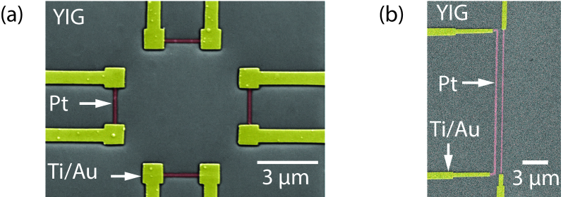
Figure 1: Colored scanning electron microscope (SEM) images of typical devices for (a) MPHE and (b) MAMR measurement. The yellow-colored structures are Ti/Au contacts and pink-colored ones are Pt strips. The grey background is the YIG substrate.

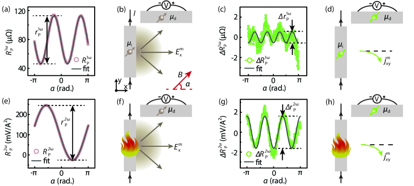
Figure 2: MPHE measurements for a typical device (series I, sample C, device 1). (a)-(d) First harmonic signal (electrical injection). (e)-(h) Second harmonic signal (thermal injection). (a), (b), (e), (f) Detection of the isotropic magnon current driven by the magnon chemical potential gradient, such as $E_{\textrm{x}}^{\textrm{m}}$. (c), (d), (g), (h) Detection of the MPHE current, $j_{\textrm{xy}}^{\textrm{m}}$. We perform a $\pi$ and $2\pi$ period sinusoidal fit for the measured $R^{1\omega}_{\textrm{P}}$ and $R^{2\omega}_{\textrm{P}}$ in (a) and (e). The residues of the fits are shown in (c) and (g) as $\Delta R^{1\omega}_{\textrm{P}}$ and $\Delta R^{2\omega}_{\textrm{P}}$, i.e. subtracting the $\pi$ and $2\pi$ period sinusoidal function from $R^{1\omega}_{\textrm{P}}$ and $R^{2\omega}_{\textrm{P}}$, respectively. Solid lines in (c) and (g) represent sinusoidal fits with period of $\pi/2$ and $2\pi/3$. The peak-to-peak amplitudes of the modulations are indicated as $r^{1\omega}_{\textrm{P}}$, $\Delta r^{1\omega}_{\textrm{P}}$, $r^{2\omega}_{\textrm{P}}$ and $\Delta r^{2\omega}_{\textrm{P}}$ in (a), (c), (e) and (g), respectively. (b), (d), (f), (h) Schematic illustration of a device top-view and measurement configuration. $\mu_{\textrm{i}}$ indicates the effective component of the magnon injection which is parallel to the magnetization aligned by B (40 mT), while $\mu_{\textrm{d}}$ denotes the component sensored by the detector. In (b) and (f), the brown clouds represent isotropic magnon diffusion from the midpoint of the injector (in reality, the whole injector strip functions). In (f) and (h), the fire represents thermal injection of Joule heating from the electrical charge current.

Magnons, or spin wave quanta, are the elementary excitations of magnetically ordered systems Chumak et al. (2015). For long wavelength GHz spin waves, the dipolar interaction plays an important role, which is intrinsically anisotropic. This results in the anisotropic transport behavior for spin waves excited via microwave field Kobljanskyj et al. (2015). In contrast, for short wavelength THz spin waves, the Heisenberg exchange energy, i.e. $-J\,\textbf{S}_{\textrm{i}}\cdot\textbf{S}_{\textrm{j}}$, dominates the dispersion, resulting in isotropic magnon propagation. However, the asymmetric spin-orbital coupling, such as Dzyaloshinskii-Moriya interaction, can cause anisotropic transport of exchange magnons Dzialoshinskii (1957); Moriya (1960); Manchon et al. (2014).

Here, we report the observation of the PHE and AMR for magnon currents in a magnetic insulator at room temperature, the magnon planar Hall effect (MPHE) and magnon anisotropic magnetoresistance (MAMR), respectively. Magnons can carry both spins and heat. Since the 1960s, the thermal properties of magnetic insulators have been extensively studied to investigate spin wave transport Akhiezer and Shishkin (1958); Bar’yakhtar and Urushadze (1961); Lüthi (1962); Douthett and Friedberg (1961); Douglass (1963); Shinozaki (1961). For example, Douglass Douglass (1963) reported the anisotropic heat conductivities of the single crystal bulk ferrimagnetic insulator yttrium iron garnet (Y₃Fe₅O₁₂, YIG) with respect to the magnetic field at 0.5 K.

Recently, it has been reported that high energy exchange magnons ($E\sim k_{\textrm{B}}T$) can be excited thermally Cornelissen et al. (2015); Giles et al. (2015); Shan et al. (2016) and electrically Cornelissen et al. (2015); Goennenwein et al. (2015); Vélez et al. (2016); Ganzhorn et al. (2016) and detected electrically in lateral non-local devices on YIG thin films. Later on, spin injection and detection in vertical sandwich devices was shown Li et al. (2016); Wu et al. (2016). The magnon transport can be described by a diffusion-relaxation equation, with a characteristic magnon relaxation length of $\lambda_{\textrm{m}}\sim 10\,$$\mu$m for both electrically and thermally excited magnons at room temperature Cornelissen et al. (2015). In this Letter our aim is to use this newly established electrical approach Cornelissen et al. (2015) to study the magnetotransport properties for exchange magnons in a magnetic insulator, where charge transport is prohibited due to the bandgap.

Typical devices used in our MPHE and MAMR measurements are shown in Fig.  1. They are fabricated on single-crystal (111) YIG films with thickness of $100\,$nm (series I) and $200\,$nm (series II). The saturation magnetization $M_{\textrm{s}}$ and Gilbert damping parameter $\alpha$ are comparable for the YIG samples in two series ($\mu_{0}M_{\textrm{s}}\sim 170\,$mT, $\alpha\sim 1\times 10^{-4}$). The YIG films are grown on a $500\,\mu$m thick (111) Gd₃Ga₅O₁₂ (GGG) substrate by liquid-phase epitaxy and obtained commercially from Matesy GmbH. The Pt electrodes are defined using electron beam lithography followed by dc sputtering in Ar⁺ plasma. The thickness of Pt layer is $\sim 7\,$nm. The Ti/Au ($5/75\,$nm) contacts are deposited by electron beam evaporation. Seven YIG samples are used with multiple devices on each of them. An overview of all devices is given in Supplementary Material VI liu .

Here, we use the electrical/thermal magnon excitation and electrical magnon detection method with Pt injectors/detectors on top of YIG as described in Ref.  Cornelissen et al. (2015). A low frequency ($\omega/2\pi=17.5\,$Hz) ac-current $I$ is sent through one Pt strip. It generates magnons in the YIG in two ways. First, the electrical current induces a transverse spin current due to spin Hall effect (SHE) Hirsch (1999); Hoffmann (2013). This results in electron spin accumulation at the Pt$\mid$YIG interface, which can excite magnons in magnetic insulators via spin-flip scattering at the interface Zhang and Zhang (2012). This is known as electrical magnon injection. Second, the Joule heating from the electrical current can thermally excite magnons via the bulk spin Seebeck effect Shan et al. (2016). Other strips are used as magnon detectors, in which the spin current flowing into the detector is converted to a voltage signal due to the inverse spin Hall effect (ISHE) Saitoh et al. (2006). Using lock-in technique, the electrically and thermally excited magnons can be measured as the first and second harmonic voltages separately. They scale linearly and quadratically with the current, i.e. $V^{1\omega}\sim I$ and $V^{2\omega}\sim I^{2}$, respectively (see Appendix A in Ref.  Vlietstra et al. (2014)). Here, we normalize them by $I$ as non-local resistances ($R^{1\omega}=V^{1\omega}/I$ and $R^{2\omega}=V^{2\omega}/I^{2}$).

For the MPHE measurements, we use an injector and detector which are perpendicular to each other, while MAMR measurements employ a detector parallel to the injector. The magnon chemical potential gradient Cornelissen et al. (2016a), which is created by the non-equilibrium magnons excited by the injector, drives the diffusion of the magnons in YIG. We define the direction which is perpendicular to the injector strip as the longitudinal direction with $E_{\textrm{x}}^{\textrm{m}}$ being the longitudinal magnon chemical potential gradient. We measure the transverse and longitudinal magnon currents with current densities of $j_{\textrm{xy}}^{\textrm{m}}$ and $j_{\textrm{xx}}^{\textrm{m}}$, i.e. the number of magnons passing through per unit cross-sectional area per second (see Figs.  2(b), 2(d)) and 3(a)).

Different from the PHE and AMR measurement for charge currents, we measure the magnetization direction dependent currents instead of the voltages. This is confirmed by the geometric reduction of the non-local signal by increasing the distance between Pt injector and detector on top of YIG within the diffusion regime for magnon transport Cornelissen et al. (2015). Therefore, the nonlocal magnon transport measurement quantified by the non-local resistances detects the magnon conductivity $\sigma^{\textrm{m}}$ instead of the resistivity. However, in this Letter we still keep the terms, such as anisotropic magnetoresistance for MAMR, because of the analogous magnetotransport behaviors of electrons and magnons.

An in-plane magnetic field B is applied to align the magnetization of the YIG film with an angle $\alpha$. We vary $\alpha$ by rotating the sample in-plane under a static magnetic field with a stepper motor. The MPHE and MAMR currents are expected to have angular dependences of

$$j_{\textrm{xy}}^{\textrm{m}}=E_{\textrm{x}}^{\textrm{m}}\,\Delta\sigma^{\textrm{m}}\,\sin\alpha\,\cos\alpha,$$ (3)

$$j_{\textrm{xx}}^{\textrm{m}}=E_{\textrm{x}}^{\textrm{m}}(\sigma_{\perp}^{\textrm{m}}+\Delta\sigma^{\textrm{m}}\cos^{2}\alpha),$$ (4)

where $\Delta\sigma^{\textrm{m}}=\sigma_{\parallel}^{\textrm{m}}-\sigma_{\perp}^{\textrm{m}}$. $\sigma_{\parallel}^{\textrm{m}}$ and $\sigma_{\perp}^{\textrm{m}}$ are conductivites for the magnon currents parallel and perpendicular to the magnetization direction, respectively.

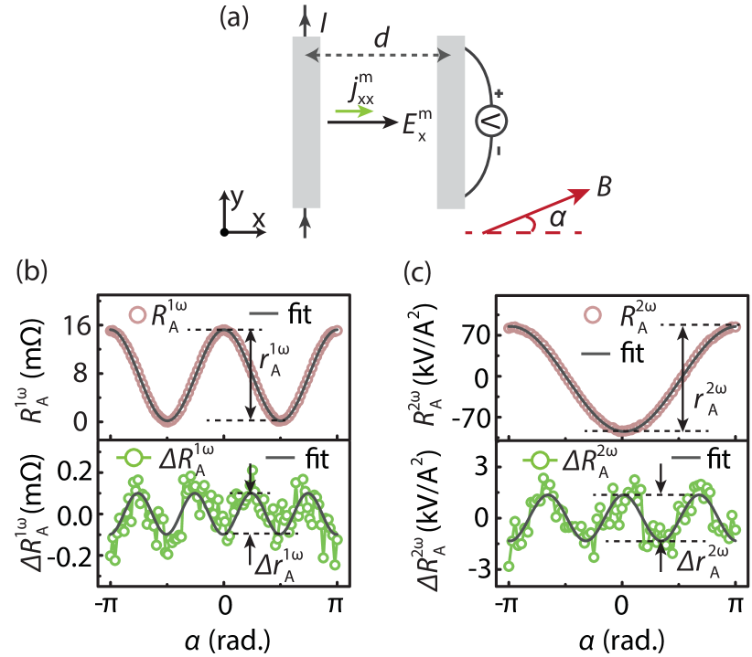
Figure 3: MAMR measurement for a typical device (series II, sample F, device 1). (a) Schematic top-view of the measurement configuration. The spacing between injector and detector is indicated as $d$. (b) First and (c) second harmonic signals with $d=200\,$nm, i.e. $R^{1\omega}_{\textrm{A}}$ and $R^{2\omega}_{\textrm{A}}$. The solid lines are $\pi$- and $2\pi$-period sinusoidal fits. In the lower panels of (b) and (c), the residues of the fits, i.e. the difference between data and corresponding fits, are shown as $\Delta R^{1\omega}_{\textrm{A}}$ and $\Delta R^{2\omega}_{\textrm{A}}$. They are fitted with $\pi/2$- and $2\pi/3$-period sinusoidal functions, respectively. $B=20\,$mT.

The result of the first harmonic MPHE measurement for electrically injected magnons in Fig.  2(a) shows mainly a $\pi$-period angular dependence. This is already discussed in prior works Cornelissen et al. (2015) and shown in Fig.  2(b). A charge current is sent through the injector, by which a spin accumulation is created at the Pt$\mid$YIG interface via the SHE. The effective component for the magnon injection, i.e. $\mu_{\textrm{i}}$, is parallel to the magnetization. This results in a $\cos\alpha$ injection efficiency Cornelissen et al. (2015). An isotropically diffusing magnon current propagates along the magnon chemical potential gradient Cornelissen et al. (2016a), being directly detected as $\mu_{d}$. Due to the ISHE, a charge voltage is measured with an efficiency of $\sin\alpha$. Taking both injection and detection into account, we end up with a $\pi$-period sinusoidal modulation

$$R^{1\omega}_{\textrm{P}}\sim C^{1\omega}\sigma_{0}^{\textrm{m}}\cos\alpha\sin\alpha=\frac{1}{2}C^{1\omega}\sigma_{0}^{\textrm{m}}\sin 2\alpha,$$ (5)

which corresponds to the angular dependence shown in Fig.  2(a). $C^{1\omega}$ is a constant related to electrical magnon injection and detection efficiency and $\sigma_{0}^{\textrm{m}}$ is average magnon current conductivity. Details are explained in Supplementary Material II liu (including Ref. Cornelissen and van Wees (2016)).

For the residue of the $\pi$-period sinusoidal fit, i.e. the discrepancy between the data and fit (Fig.  2(c)), there is a $\pi/2$-period sinusoidal modulation in the first harmonic signals. This is ascribed to the existence of the MPHE as illustrated in Fig.  2(d). The MPHE induces an additional $\pi$-period angular dependence as indicated in Eq.  (3). Together with the injection-detection efficiencies described in Eq. (5), i.e. $(C^{1\omega}\cos\alpha\,\sin\alpha)\,(\Delta\sigma^{\textrm{m}}\sin\alpha\,\cos\alpha)$, it results in a component in the first harmonic resistance with an angular dependence of

$$\Delta R^{1\omega}_{\textrm{P}}\sim-\frac{1}{8}C^{1\omega}\Delta\sigma^{\textrm{m}}\cos 4\alpha.$$ (6)

This corresponds to the $\pi/2$-period modulation in Fig.  2(c).

For the second harmonic MPHE measurement, the thermal injection due to the Joule heating is insensitive to the YIG magnetization. Therefore, the thermally excited magnons can be directly detected as electron spins with polarization parallel to the magnetization as $\mu_{\textrm{d}}$ (c.f. Fig.  2(f)) with a detection efficiency of $\sin\alpha$

$$R^{2\omega}_{\textrm{P}}\sim C^{2\omega}\sigma_{0}^{\textrm{m}}\sin\alpha,$$ (7)

which corresponds to the $2\pi$-period modulation in Fig.  2(e). $C^{2\omega}$ is a parameter describing the thermal injection and electrical detection efficiency which is explained further in Supplementary Material II liu . Since the electrically and thermally excited magnons show a similar $\lambda_{\textrm{m}}$ over a wide temperature range Cornelissen et al. (2015, 2016b) and a similar magnetic field dependent behaviour Cornelissen and van Wees (2016), this strongly suggests that the same exchange magnons are involved in the spin transport. Therefore, we assign the same conductivities $\sigma_{0}^{\textrm{m}}$ and $\Delta\sigma^{\textrm{m}}$ to electrically and thermally excited magnons.

Similarly, by looking at the deviation of the data from the $2\pi$-period modulation, a $2\pi/3$-period oscillation is observed in Fig.  2(g). When the thermal magnons also experience the MPHE, i.e. $(C^{2\omega}\,\sin\alpha)\,(\Delta\sigma^{\textrm{m}}\sin\alpha\,\cos\alpha)$, we expect a component in the second harmonic signal as

$$\Delta R^{2\omega}_{\textrm{P}}\sim-\frac{1}{4}C^{2\omega}\Delta\sigma^{\textrm{m}}\cos 3\alpha,$$ (8)

which conforms to the $2\pi/3$-period oscillation in Fig.  2(g). Besides, we also did MPHE measurement by using two detectors which are symmetrically patterned with respect to the injector, where we obtain the doubled asymmetric MPHE-current and the suppressed isotropic magnon current due to symmetry. Also, it excludes the influence of the asymmetric potential gradient in the single detector case (explained in detail in Supplementary Material III liu ).

To quantify the MPHE, we extract the peak-to-peak amplitude of $R^{1\omega}_{\textrm{P}}$, $\Delta R^{1\omega}_{\textrm{P}}$, $R^{2\omega}_{\textrm{P}}$ and $\Delta R^{2\omega}_{\textrm{P}}$ as $r_{\textrm{P}}^{1\omega}$, $\Delta r_{\textrm{P}}^{1\omega}$, $r_{\textrm{P}}^{2\omega}$ and $\Delta r_{\textrm{P}}^{2\omega}$ by using

$$R^{1\omega}_{\textrm{P}}=\frac{1}{2}r_{\textrm{P}}^{1\omega}\,\sin(2\alpha+\alpha_{1})+R_{1},$$ (9)

$$\Delta R^{1\omega}_{\textrm{P}}=-\frac{1}{2}\Delta r_{\textrm{P}}^{1\omega}\,\cos(4\alpha+\alpha_{2})+R_{2},$$ (10)

$$R^{2\omega}_{\textrm{P}}=\frac{1}{2}r_{\textrm{P}}^{2\omega}\,\sin(\alpha+\alpha_{3})+R_{3},$$ (11)

$$\Delta R^{2\omega}_{\textrm{P}}=-\frac{1}{2}\Delta r_{\textrm{P}}^{2\omega}\,\cos(3\alpha+\alpha_{4})+R_{4},$$ (12)

with angle shifts indicated as $\alpha_{1},\alpha_{2},\alpha_{3}$ and $\alpha_{4}$, and offsets expressed as $R_{1},R_{2},R_{3}$ and $R_{4}$. They vary in different device geometries and measurement configuration. Further details are explained in Supplementary Material I liu .

We obtain the magnitude of the MPHE as $\Delta\sigma^{\textrm{m}}/\sigma^{\textrm{m}}_{0}$ by determining $\Delta r^{\textrm{n}\omega}_{\textrm{P}}/r^{\textrm{n}\omega}_{\textrm{P}}$ according to approximate Eqs. (5)-(8) and Eqs. (9)-(12)

$$\frac{\Delta\sigma^{\textrm{m}}}{\sigma^{\textrm{m}}_{0}}\approx\frac{4\,\Delta r^{1\omega}_{\textrm{P}}}{r^{1\omega}_{\textrm{P}}},$$ (13)

$$\frac{\Delta\sigma^{\textrm{m}}}{\sigma^{\textrm{m}}_{0}}\approx\frac{4\,\Delta r^{2\omega}_{\textrm{P}}}{r^{2\omega}_{\textrm{P}}},$$ (14)

for the first and second harmonic signals, respectively. For the derivation, see Supplementary Materials II liu . For the results shown in Fig. 2, we extract the magnitude of $|\Delta\sigma^{\textrm{m}}/\sigma^{\textrm{m}}_{0}|$ as $(6.6\pm 0.6)\,\%$ and $(4.7\pm 0.2)\,\%$ for the first and second harmonic signals, respectively. Regarding the sign, we observe that $\Delta\sigma^{\textrm{m}}<0$, i.e. $\sigma_{\parallel}^{\textrm{m}}<\sigma_{\perp}^{\textrm{m}}$, for both first and second harmonic signals, since $r^{1\omega}_{\textrm{P}}$, $r^{2\omega}_{\textrm{P}}<0$ and $\Delta r^{1\omega}_{\textrm{P}}$, $\Delta r^{2\omega}_{\textrm{P}}>0$ in Fig. 2. This sign agrees with the results of the heat conductivity measurement on the single crystal YIG at low temperature, when mainly magnons carry the heat Douglass (1963).

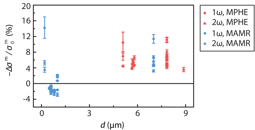
Figure 4: Sign and amplitude of the MPHE and MAMR measurements. $-\Delta\sigma^{\textrm{m}}/\sigma^{\textrm{m}}_{0}$ as a function of the injector-to-detector spacing $d$. Solid circles and triangles denote the first and second harmonic signals, i.e. $1\omega$ and $2\omega$, while pink and blue colors represent MPHE and MAMR results, respectively. $-\Delta\sigma^{\textrm{m}}>0$ means $\sigma_{\perp}^{\textrm{m}}>\sigma_{\parallel}^{\textrm{m}}$. The sign anomaly appears for the MAMR devices with $d\in[{0.2,1.0}]\,\mu$m. In this regime, the magnitude of $-\Delta\sigma^{\textrm{m}}/\sigma^{\textrm{m}}_{0}$ is comparably smaller. Without considering the data with the anomalous sign, we calculate the average value of $-\Delta\sigma^{\textrm{m}}/\sigma^{\textrm{m}}_{0}$ as $(6.1\pm 2.1)\%$ and $(5.0\pm 4.0)\%$ for the MPHE and MAMR, respectively. For the MPHE device, $d$ is defined as the spacing between the middle points of the injector and detector.

In the MAMR measurements, we also observe the characteristic period for the first and second harmonic signals, a $\pi/2$-period and a $2\pi/3$-period angular modulation, respectively (see Figs.  3(b) and 3(c)). For the magnitude of the MAMR results, we can extract the peak-to-peak amplitudes of $R^{1\omega}_{\textrm{A}}$, $\Delta R^{1\omega}_{\textrm{A}}$, $R^{2\omega}_{\textrm{A}}$, $\Delta R^{2\omega}_{\textrm{A}}$ as $r^{1\omega}_{\textrm{A}}$, $\Delta r^{1\omega}_{\textrm{A}}$, $r^{2\omega}_{\textrm{A}}$, $\Delta r^{2\omega}_{\textrm{A}}$ from the results shown in Fig. 3. We obtain $|\Delta\sigma^{\textrm{m}}/\sigma^{\textrm{m}}_{0}|$ as $(5.3\pm 0.6)\,\%$ and $(5.9\pm 0.6)\,\%$ for the first and second harmonic signals with the same sign of $\sigma_{\parallel}^{\textrm{m}}<\sigma_{\perp}^{\textrm{m}}$.

The sign and magnitude of all the measured MPHE and MAMR are summarized in Fig. 4. On different samples and devices, all the MPHE devices show the sign of $\sigma_{\perp}^{\textrm{m}}>\sigma_{\parallel}^{\textrm{m}}$ for both first and second harmonic signals. However, as can be seen in Fig. 4, for the MAMR measurement, the oppsite sign and weaker effect arises when the injector-to-detector spacing is in the range of $[{0.2,1.0}]\,\mu$m. We do not understand, why the sign and magnitude anomaly appears in this range. More details are described in Supplementary Material VI liu .

We exclude possible extra modulations induced by the misalignment between the magnetic field and in-plane magnetization angle due to the anisotropy or sample misalignment as described in Supplementary Materials IV and V liu (including Refs. Wang et al. (2014); Meyer et al. (2016); Spaldin (2010); Wang and Zeng (1986)). Besides, we check the reciprocity and linearity for $R^{1\omega}$ and $\Delta R^{1\omega}$ in Supplementary Materials VII liu .

To conclude, we observe MPHE and MAMR for both electrically and thermally injected magnons from the angular dependent transverse and longitudinal non-local measurement at room temperature. The magnitude of these effects, $|\Delta\sigma^{\textrm{m}}/\sigma_{0}^{\textrm{m}}|$, is approximately 5% for both electrically and thermally injected magnons on YIG thin films, which is in the same order of magnitude as that of PHE or AMR in ferromagnetic metals. We observe that $\sigma_{\perp}^{\textrm{m}}>\sigma_{\parallel}^{\textrm{m}}$ for all the measured devices except those MAMR devices with certain injector-to-detector spacing. This is similar to the electronic magnetoresistance of most metallic systems ($\rho_{\parallel}^{\textrm{c}}>\rho_{\perp}^{\textrm{c}}$). Our results establish a new way to study and employ the magnetotransport of magnons, which can give an insight into the spin-orbital interaction of insulating materials.

We acknowledge H. M. de Roosz, J. G. Holstein, H. Adema and T. J. Schouten for their technical assistance and appreciate M. Mostovoy, T.T.M Palstra, I. J. Vera Marun, J. Mendil and R. Schlitz for discussion. This work is part of the research programme of the Foundation for Fundamental Research on Matter (FOM) and supported by NanoLab NL and the Zernike Institute for Advanced Materials. Further support by EU FP7 ICT Grant No. 612759 InSpin and the Deutsche Forschungsgemeinschaft (DFG) within the priority program Spin Caloric Transport (SPP 1538, KU3271/1-1) is gratefully acknowledged.

References

- Thomson (1856) W. Thomson, Proc. R. Soc. London 8, 546 (1856).
- Kondo (1962) J. Kondo, Prog. Theor. Phys. 27, 772 (1962).
- Ky (1966) V.-D. Ky, Sov. Phys. JETP 23 (1966).
- Ky (1967) V.-D. Ky, Phys. Status Solidi B 22, 729 (1967).
- Kokado et al. (2012) S. Kokado, M. Tsunoda, K. Harigaya, and A. Sakuma, J. Phys. Soc. Jpn. 81, 024705 (2012).
- Livingston (1996) J. D. Livingston, Driving force: the natural magic of magnets (Harvard University Press, 1996).
- Freitas et al. (2007) P. P. Freitas, R. Ferreira, S. Cardoso, and F. Cardoso, J. Phys. Condens. Matter 19, 165221 (2007).
- McGuire and Potter (1975) T. R. McGuire and R. I. Potter, IEEE Trans. Magn. 11, 1018 (1975).
- Chumak et al. (2015) A. V. Chumak, V. I. Vasyuchka, A. A. Serga, and B. Hillebrands, Nat. Phys. 11, 453 (2015).
- Kobljanskyj et al. (2015) Y. V. Kobljanskyj, G. A. Melkov, A. A. Serga, A. N. Slavin, and B. Hillebrands, Phys. Rev. Appl. 4, 014014 (2015).
- Dzialoshinskii (1957) I. E. Dzialoshinskii, Sov. Phys. JETP 5, 1259 (1957).
- Moriya (1960) T. Moriya, Phys. Rev. 120, 91 (1960).
- Manchon et al. (2014) A. Manchon, P. B. Ndiaye, J.-H. Moon, H.-W. Lee, and K.-J. Lee, Phys. Rev. B 90, 224403 (2014).
- Akhiezer and Shishkin (1958) A. I. Akhiezer and L. A. Shishkin, Sov. Phys. JETP 34 (1958).
- Bar’yakhtar and Urushadze (1961) V. G. Bar’yakhtar and G. I. Urushadze, Sov. Phys. JETP 12 (1961).
- Lüthi (1962) B. Lüthi, J. Phys. Chem. Solids 23, 35 (1962).
- Douthett and Friedberg (1961) D. Douthett and S. A. Friedberg, Phys. Rev. 121, 1662 (1961).
- Douglass (1963) R. L. Douglass, Phys. Rev. 129, 1132 (1963).
- Shinozaki (1961) S. S. Shinozaki, Phys. Rev. 122, 388 (1961).
- Cornelissen et al. (2015) L. J. Cornelissen, J. Liu, R. A. Duine, J. Ben Youssef, and B. J. van Wees, Nat. Phys. 11, 1022 (2015).
- Giles et al. (2015) B. L. Giles, Z.-H. Yang, J. S. Jamison, and R. C. Myers, Phys. Rev. B 92, 224415 (2015).
- Shan et al. (2016) J. Shan, L. J. Cornelissen, N. Vlietstra, J. Ben Youssef, T. Kuschel, R. A. Duine, and B. J. van Wees, Phys. Rev. B 94, 174437 (2016).
- Goennenwein et al. (2015) S. T. B. Goennenwein, R. Schlitz, M. Pernpeintner, K. Ganzhorn, M. Althammer, R. Gross, and H. Huebl, Appl. Phys. Lett. 107, 172405 (2015).
- Vélez et al. (2016) S. Vélez, A. Bedoya-Pinto, W.-J. Yan, L. E. Hueso, and F. Casanova, Phys. Rev. B 94, 174405 (2016).
- Ganzhorn et al. (2016) K. Ganzhorn, S. Klingler, T. Wimmer, S. Geprägs, R. Gross, H. Huebl, and S. T. B. Goennenwein, Appl. Phys. Lett. 109, 022405 (2016).
- Li et al. (2016) J.-X. Li, Y.-D. Xu, M. Aldosary, C. Tang, Z.-S. Lin, S.-F. Zhang, R. Lake, and J. Shi, Nat. Commun. 7 (2016).
- Wu et al. (2016) H. Wu, C.-H. Wan, X. Zhang, Z.-H. Yuan, Q.-T. Zhang, J.-Y. Qin, H.-X. Wei, X.-F. Han, and S.-F. Zhang, Phys. Rev. B 93, 060403 (2016).
- (28) See Supplemental Material for more detailed information and data supplemental to the main article .
- Hirsch (1999) J. E. Hirsch, Phys. Rev. Lett. 83, 1834 (1999).
- Hoffmann (2013) A. Hoffmann, IEEE Trans. Magn. 49, 5172 (2013).
- Zhang and Zhang (2012) S. S.-L. Zhang and S.-F. Zhang, Phys. Rev. Lett. 109, 096603 (2012).
- Saitoh et al. (2006) E. Saitoh, M. Ueda, H. Miyajima, and G. Tatara, Appl. Phys. Lett. 88, 182509 (2006).
- Vlietstra et al. (2014) N. Vlietstra, J. Shan, B. J. van Wees, M. Isasa, F. Casanova, and J. Ben Youssef, Phys. Rev. B 90, 174436 (2014).
- Cornelissen et al. (2016a) L. J. Cornelissen, K. J. H. Peters, G. E. W. Bauer, R. A. Duine, and B. J. van Wees, Phys. Rev. B 94, 014412 (2016a).
- Cornelissen and van Wees (2016) L. J. Cornelissen and B. J. van Wees, Phys. Rev. B 93, 020403 (2016).
- Cornelissen et al. (2016b) L. J. Cornelissen, J. Shan, and B. van Wees, Phys. Rev. B 94, 180402 (2016b).
- Wang et al. (2014) H.-L. Wang, C.-H. Du, P. C. Hammel, and F.-Y. Yang, Phys. Rev. B 89, 134404 (2014).
- Meyer et al. (2016) S. Meyer, Y.-T. Chen, S. Wimmer, M. Althammer, S. Geprägs, H. Huebl, D. Ködderitzsch, H. Ebert, G. E. W. Bauer, R. Gross, et al., arXiv preprint arXiv:1607.02277 (2016).
- Spaldin (2010) N. A. Spaldin, Magnetic materials: fundamentals and applications (Cambridge University Press, 2010).
- Wang and Zeng (1986) Y.-Q. Wang and X.-Y. Zeng, Hyperfine Interact. 28, 447 (1986).