On fixed-parameter tractability of the mixed domination problem for graphs with bounded tree-width

Abstract

A mixed dominating set for a graph $G=(V,E)$ is a set $S\subseteq V\cup E$ such that every element $x\in(V\cup E)\backslash S$ is either adjacent or incident to an element of $S$. The mixed domination number of a graph $G$, denoted by $\gamma_{m}(G)$, is the minimum cardinality of mixed dominating sets of $G$. Any mixed dominating set with the cardinality of $\gamma_{m}(G)$ is called a minimum mixed dominating set. The mixed domination set (MDS) problem is to find a minimum mixed dominating set for a graph $G$ and is known to be an NP-complete problem. In this paper, we present a novel approach to find all of the mixed dominating sets, called the AMDS problem, of a graph with bounded tree-width $w$. Our new technique of assigning power values to edges and vertices, and combining with dynamic programming, leads to a fixed-parameter algorithm of time $O(3^{w^{2}}\times w^{2}\times|V|)$. This shows that MDS is fixed-parameter tractable with respect to tree-width. In addition, we theoretically improve the proposed algorithm to solve the MDS problem in $O(6^{w}\times|V|)$ time.

1 Introduction

The mixed dominating set (MDS) problem was first introduced in 1977 by Alavi et. al. Alavi et al. (1977). The MDS problem has many practical applications such as placing phase measurement units in an electric power system Zhao et al. (2011). Also, there are variations and generalizations of the MDS such as Roman MDS and signed Roman MDS which were introduced and studied by Abdollahzadeh et al. Ahangar et al. (2015b, a).

An edge dominates its endpoints as well as all of its adjacent edges. Also, a vertex dominates all of its neighboring vertices as well as all of its incident edges. Formally, a set $S\subseteq V\cup E$ of vertices and edges of a graph $G=(V,E)$ is called a MDS if every element $x\in(V\cup E)\setminus S$ is dominated by an element of $S$. The mixed domination number of $G$ is the size of the smallest mixed dominating set of $G$ and is denoted by $\gamma_{m}(G)$. Finding all of the mixed dominating set of a graph is called AMDS problem.

The MDS problem is NP-complete for general graphs Zhao et al. (2011). There exist different approaches to solve an NP-complete problem such as approximation, randomization, heuristics, and parameterization. Several approximation algorithms exist for solving the MDS problem such as a 2-factor one by Hatami Hatami (2007). It is notable that the MDS problem remains NP-complete even for split graphs due to the high tree-width of the input graph Lan and Chang (2013); however, the MDS problem is polynomial tractable for cacti and trees Lan and Chang (2013). A parallel concept is proposed by Adhar et al. in Adhar and Peng (1994) which requires $O(n)$ processors in CRCW PRAM model to solve the MDS in $O(\log n)$ time where $n$ is the number of graph vertices.

The parameterization method is a well-known technique which considers certain parameters on the input constant to get a polynomial time algorithm with respect to the size of the input and may contain exponential terms with respect to these fixed parameters. A famous example of such parameters is the tree-width which was introduced by Robertson and Seymour in 1984 Robertson and Seymour (1984). The tree-width parameter has proven to be a good coping strategy for tackling the intrinsic difficulty for various NP-hard problems on graphs. The tree-width measures the similarity of a graph to a tree. Since most of the algorithms work efficiently on trees, the tree decomposition of a graph can be used to speed up solving some problems on graphs with a small tree-width. Although some problems in graph theory cannot be solved in polynomial time even with respect to some fixed parameter, there are many other interesting problems in graph theory which are fixed parameter tractable (FPT). To show that a problem is FPT, one existing way is to express the problem in monadic second-order logic; if a problem can be modeled in this way, then it is FPT by Courcelle’s famous theorem Courcelle (1992, 2015). The reduction technique, which is an extension of a graph reduction to another graph of bounded tree-width by Bodlaender (see Bodlaender and van Antwerpen-de Fluiter (2001)), is another technique which helps solving problems in linear time with respect to constant tree-width.

Almost all of the algorithmic approaches that consider the input graph of a constant tree-width use the dynamic programming paradigm. For example, Chimani proposed an algorithm to solve the Steiner tree problem using dynamic programming Chimani et al. (2012).

In Rajaati et al. (2016), we proposed an approach to solve the problem of finding all of the mixed dominating sets (AMDS) for a graph $G=(V,E)$ of bounded tree-width $w$ which has time complexity $O(3^{w^{2}}\times w^{2}\times|V|)$. Our constructive algorithm shows that the MDS is fixed-parameter tractable with respect to tree-width. As defined later, the fundamental idea we use to solve the MDS problem is to assign power values to vertices. Recently, Jain et al. in Jain et al. (2017) enhanced the complexity of Rajaati et al. (2016) to $O^{*}(6^{w})$. Here they showed how to turn any set $S\subseteq V\cup E$ to satisfy $(i)$ the edges in $S$ form a matching, and $(ii)$ the set of endpoints of edges in $S$ is disjoint from the vertices in $S$, to a minimum sized mixed dominating set. In this paper, we also modify our original proposed algorithm of Rajaati et al. (2016) to solve MDS with time complexity $O^{*}(6^{w})$.

The rest of the paper is organized as follows: In Section 2, we give necessary notations and definitions. In Section 3, we define the concept of charging vertices which is a key part of our proposed algorithm. Our proposed algorithm that solves the AMDS is presented in Section 4. Then, we modify this algorithm to solve MDS. In Section 5, we formally show the correctness of the proposed algorithm. Finally, a brief conclusion and ideas for future work are discussed in Section 6.

2 Preliminaries

In this section, we overview the graph theory that is used throughout the paper. In general, the notation used below follows West et al. (2001) and Haynes et al. (1998).

All graphs considered in this paper are undirected and simple, i.e. no parallel edges or self-loops. Let $G=(V,E)$ be a graph with the vertex set $V$ and the edge set $E$.

For vertex $v\in V$, $N(v)$ denotes the open neighborhood of $v$ and is defined as $N(v)=\{u\in V\mid uv\in E\}$. The edge open neighborhood of the vertex $v$ is defined as $N^{e}(v)=\{e\in E\mid e=uv\}$. Also, for an edge $e=uv\in E$, $N(e)=\{u,v\}$ denotes the open neighborhood of $e$. The edge open neighborhood of the edge $e=uv$ is defined as $N^{e}(e)=\{e^{\prime}\in E\mid e^{\prime}=uv^{\prime}$ or $e^{\prime}=u^{\prime}v$ where $u\not=u^{\prime}$ and $v\not=v^{\prime}\}$. We denote the mixed neighborhood of vertex $v$ by $N^{md}(v)$ such that $N^{md}(v)=N(v)\cup N^{e}(v)$, and the mixed neighborhood of edge $e$ by $N^{md}(e)$ such that $N^{md}(e)=N(e)\cup N^{e}(e)$. Finally, for any element $r\in V\cup E$, we denote the mixed neighborhood of $r$ by $N^{md}_{G}(r)$. Also, for any element $r\in V\cup E$, the closed mixed neighborhood is defined as $N^{md}_{G}(r)\cup\{r\}$ and is denoted by $N^{md}_{G}[r]$.

A tree decomposition of a graph $G$ is a mapping of $G$ into a tree $T$ which satisfies certain properties. Note that throughout the paper, nodes of $G$ are called vertices while nodes of $T$ are called bags.

Definition 2.1.

Let $G=(V,E)$ be a graph. A tree decomposition of $G$ is a pair $(\mathcal{X}=\{X_{i}\mid i\in\mathcal{I}\},T)$, where each $X_{i}$ is a subset of $V$, which is called a bag, $T$ is a tree with elements of $\mathcal{I}$ as bags and satisfies the following three properties.

1. $\bigcup_{i\in\mathcal{I}}X_{i}=V$,

2. for every edge $\{u,v\}\in E$, there is an index $i\in\mathcal{I}$ such that $\{u,v\}\subseteq X_{i}$,

3. for all $i,j,k\in\mathcal{I}$, if $j$ lies on the path between $i$ and $k$ in $T$, then $X_{i}\cap X_{k}\subseteq X_{j}$.

The width of a tree decomposition $(\mathcal{X}=\{X_{i}\mid i\in\mathcal{I}\},T)$ equals to $\max\{|X_{i}|\mid i\in\mathcal{I}\}-1$. The tree-width of a graph $G$, denoted by $w$, is the minimum width among all the tree decompositions of graph $G$.

Definition 2.2.

A tree decomposition $(\mathcal{X}=\{X_{i}\mid i\in\mathcal{I}\},T)$ is called a nice tree decomposition if the following conditions are met:

1. Every bag of the tree has at most two children.

2. If a bag $i$ has two children $j$ and $k$, then $X_{i}=X_{j}=X_{k}$. Such a bag is called a join bag.

3. If a bag $i$ has exactly one child like $j$, then one of the following conditions must hold:

   (a)

   $|X_{i}|=|X_{j}|+1$ and $X_{j}\subset X_{i}$

   (b)

   $|X_{i}|=|X_{j}|-1$ and $X_{i}\subset X_{j}$

   Note that if (a) holds, the bag $|X_{i}|$ is called an introduce bag, and if (b) holds, it is called a forget bag.

Lemma 2.3.

(Bodlaender (1996)) Given a tree decomposition of a graph $G$ of width $w$, and $n$ vertices, one can find a nice tree decomposition of $G$ in linear time of width $w$ and $O(n)$ bags.

Definition 2.4.

A nice tree decomposition is called a very nice tree decomposition if each leaf bag contains just a single vertex.

(a)

(b)

Figure 1: (a) Graph $G1$, (b) One of nice tree decomposition of $G1$ with treewidth 2. The bags of tree decomposition are numbered according to a preorder traversal on it.

3 Fundamental Concepts

The fundamental idea that we use to solve the AMDS is transferring the edge power to the vertex power.

Let $\mathcal{MD}$ be a mixed domination set, $X_{i}$ be a bag in a tree decomposition of $G$ and $v\in X_{i}$ be a vertex of $G$. The rules for transferring the domination power of the edges to the vertices are as follows:

• Power 2: If $v\in\mathcal{MD}$, then the power of $v$ is set equal to 2. In this case, this vertex can dominate the elements in $N^{md}_{G}[r]$.

• Power 1: If $v\notin\mathcal{MD}$ and at least one of the incident edges of the vertex $v$ is in $\mathcal{MD}$, then the power of $v$ is set equal to $1$. This vertex can dominate all of its incident edges.

• Power 0: If $v$ and all of its incident edges are not in $\mathcal{MD}$, then the power of $v$ is set equal to $0$. This vertex cannot dominate any edges or vertices.

Given a vertex $v\in X_{i}$, there are seven situations to consider which are illustrated in the Table 1. The intuition behind each of these cases is as follows:

1. In the first case, the vertex $v$ and at least one of its incident edges belong to $\mathcal{MD}$,

2. In the second case, $v$ belong to $\mathcal{MD}$, however, none of its edges belong to $\mathcal{MD}$,

3. In the third case, $v$ does not belong to $\mathcal{MD}$ but at least one of its incident edges belongs to $\mathcal{MD}$,

4. In the fourth case, $v$ and all of its edges do not belong to $\mathcal{MD}$, and $v$ and its edges are dominated,

5. In the fifth case, $v$ and all of its edges do not belong to $\mathcal{MD}$, and $v$ is not dominated but all its edges are dominated,

6. In the sixth case, $v$ and all of its edges do not belong to $\mathcal{MD}$, and $v$ is dominated but at least one of its edges is not dominated,

7. In the seventh case, $v$ and all of its edges do not belong to $\mathcal{MD}$, and $v$ and at least one of its edges is not dominated.

Table 1: The seven possible situation for a vertex in a bag.

	$v\in\mathcal{MD}$	$N^{e}_{X_{i}}(v)\in\mathcal{MD}$	vertex cover	edge cover	vertex power	illustration
1	$v\in\mathcal{MD}$	$\exists e\in N^{e}_{X_{i}}(v),e\in\mathcal{MD}$	$v$ is covered	$\forall e\in N^{e}_{X_{i}}(v),e$ is covered	2	2(a).
2	$v\in\mathcal{MD}$	$\forall e\in N^{e}_{X_{i}}(v),e\notin\mathcal{MD}$	$v$ is covered	$\forall e\in N^{e}_{X_{i}}(v),e$ is covered	2	2(b).
3	$v\notin\mathcal{MD}$	$\exists e\in N^{e}_{X_{i}}(v),e\in\mathcal{MD}$	$v$ is covered	$\forall e\in N^{e}_{X_{i}}(v),e$ is covered	1	2(c).
4	$v\notin\mathcal{MD}$	$\forall e\in N^{e}_{X_{i}}(v),e\notin\mathcal{MD}$	$v$ is covered	$\forall e\in N^{e}_{X_{i}}(v),e$ is covered	0	2(d).
5	$v\notin\mathcal{MD}$	$\forall e\in N^{e}_{X_{i}}(v),e\notin\mathcal{MD}$	$v$ is not covered	$\forall e\in N^{e}_{X_{i}}(v),e$ is covered	0	2(e).
6	$v\notin\mathcal{MD}$	$\forall e\in N^{e}_{X_{i}}(v),e\notin\mathcal{MD}$	$v$ is covered	$\exists e\in N^{e}_{X_{i}}(v),e$ is not covered	0	2(f).
7	$v\notin\mathcal{MD}$	$\forall e\in N^{e}_{X_{i}}(v),e\notin\mathcal{MD}$	$v$ is not covered	$\exists e\in N^{e}_{X_{i}}(v),e$ is not covered	0	2(g).

In Figure 2 we illustrate these situations where a rectangle indicates a bag; the vertices or edges that are in $\mathcal{MD}$ are drawn as disk or bold line, respectively. Not covered elements are drawn by dotted lines or circles and the remaining elements are covered. In Figures 2(b), 2(d) and 2(e), we use an arc sector for incident edges of the selected vertex in the bag. It means all of the edges are covered, but in Figures 2(a) and 2(c) at least one of incident edges of the vertex is in $\mathcal{MD}$ and in Figures 2(f) and 2(g) at least one of incident edges of the vertex is not covered.

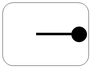
(a) 1

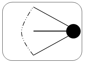
(b) 2

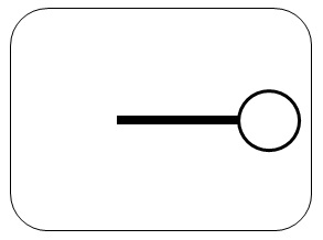
(c) 3

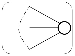
(d) 4

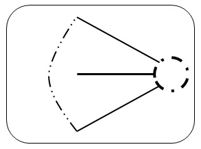
(e) 5

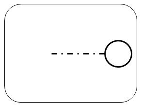
(f) 6

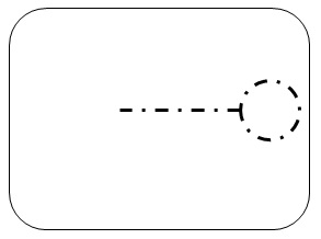
(g) 7

Figure 2: Different situations for a vertex with respect to a bag.

Let $T$ be a very nice tree decomposition (recall Definition 2.4) for the graph $G$. For each bag $X_{i}$ in $T$, we define the set $X^{\triangle}_{i}$ as

$$X^{\triangle}_{i}=\{v\in V\mid v\text{ is in the descendant bags of }X_{i}\mbox{ within }\mathcal{I}\}.$$ (1)

The induced subgraph of $G$ with vertices $X_{i}$ $(\text{or }X^{\triangle}_{i})$ is denoted by $G_{i}$ $(\text{or }G_{i}^{\triangle})$. Let $\mathcal{MD}$ be a mixed dominating set for the bag $X_{i}$ and $v\in X_{i}$. For a vertex $v$, there are nine possible situations to consider based on the intersection of $G_{i}^{\triangle}$ and bag $X_{i}$. These are given in Table 2. Assuming that all of the elements in $G_{i}^{\triangle}/G_{i}$ are dominated, seven situations of the Table 2 are the same as earlier given in Table 1. However, to cover the cases that edges in $G_{i}^{\triangle}/G_{i}$ are not dominated, two extra cases are possible for $v$.

• The vertex $v$ is dominated, however at least one of its edges in $G_{i}^{\triangle}/G_{i}$ is not dominated.

• The vertex $v$ and at least one of its edges in $G_{i}^{\triangle}/G_{i}$ are not dominated.

In both case, the vertex $v$ is not in $\mathcal{MD}$, and at least one of its incident edges in $G_{i}^{\triangle}/G_{i}$ is not dominated. However the vertex $v$ in state 8 is dominated, and in state 9 is not dominated.

Table 2: Different cases for a vertex $v\in X_{i}$ in correspondence to the edges and vertices in $X_{i}$.

	$v\in\mathcal{MD}$	$N^{e}_{X^{\triangle}_{i}}(v)\in\mathcal{MD}$	vertex cover	edge is covered in this bag	edge is covered in previous bags	power	illustration
1	$v\in\mathcal{MD}$	$\exists e\in N^{e}_{X^{\triangle}_{i}}(v),e\in\mathcal{MD}$	$v$ is covered	$\forall e\in N^{e}_{X_{i}}(v),e$ is covered	$\forall e\in N^{e}_{X^{\triangle}_{i}}(v),e$ is covered	2	Figure 3(a)
2	$v\in\mathcal{MD}$	$\forall e\in N^{e}_{X^{\triangle}_{i}}(v),e\notin\mathcal{MD}$	$v$ is covered	$\forall e\in N^{e}_{X_{i}}(v),e$ is covered	$\forall e\in N^{e}_{X^{\triangle}_{i}}(v),e$ is covered	2	Figure 3(b)
3	$v\notin\mathcal{MD}$	$\exists e\in N^{e}_{X^{\triangle}_{i}}(v),e\in\mathcal{MD}$	$v$ is covered	$\forall e\in N^{e}_{X_{i}}(v),e$ is covered	$\forall e\in N^{e}_{X^{\triangle}_{i}}(v),e$ is covered	1	Figure 3(c)
4	$v\notin\mathcal{MD}$	$\forall e\in N^{e}_{X^{\triangle}_{i}}(v),e\notin\mathcal{MD}$	$v$ is covered	$\forall e\in N^{e}_{X_{i}}(v),e$ is covered	$\forall e\in N^{e}_{X^{\triangle}_{i}}(v),e$ is covered	0	Figure 3(d)
5	$v\notin\mathcal{MD}$	$\forall e\in N^{e}_{X^{\triangle}_{i}}(v),e\notin\mathcal{MD}$	$v$ is not covered	$\forall e\in N^{e}_{X_{i}}(v),e$ is covered	$\forall e\in N^{e}_{X^{\triangle}_{i}}(v),e$ is covered	0	Figure 3(e)
6	$v\notin\mathcal{MD}$	$\forall e\in N^{e}_{X^{\triangle}_{i}}(v),e\notin\mathcal{MD}$	$v$ is covered	$\exists e\in N^{e}_{X_{i}}(v),e$ is not covered	$\forall e\in N^{e}_{X^{\triangle}_{i}}(v),e$ is covered	0	Figure 3(f)
7	$v\notin\mathcal{MD}$	$\forall e\in N^{e}_{X^{\triangle}_{i}}(v),e\notin\mathcal{MD}$	$v$ is not covered	$\exists e\in N^{e}_{X_{i}}(v),e$ is not covered	$\forall e\in N^{e}_{X^{\triangle}_{i}}(v),e$ is covered	0	Figure 3(g)
8	$v\notin\mathcal{MD}$	$\forall e\in N^{e}_{X^{\triangle}_{i}}(v),e\notin\mathcal{MD}$	$v$ is covered	$e$ is or is not covered	$\exists e\in N^{e}_{X^{\triangle}_{i}}(v),e$ is not covered	0	Figure 3(h)
9	$v\notin\mathcal{MD}$	$\forall e\in N^{e}_{X^{\triangle}_{i}}(v),e\notin\mathcal{MD}$	$v$ is not covered	$e$ is or is not covered	$\exists e\in N^{e}_{X^{\triangle}_{i}}(v),e$ is not covered	0	Figure 3(i)

The Figure 3 is similar to the Figure 2, except that it shows different situations for a vertex $v\in X_{i}$ with respect to a bag $X_{i}$, and it considers the edges and vertices appearing in previous bags.

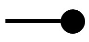
(a) 1

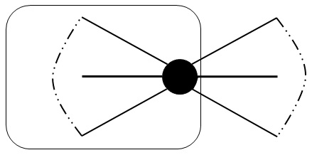
(b) 2

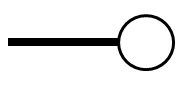
(c) 3

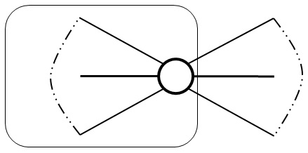
(d) 4

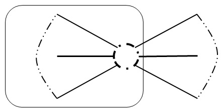
(e) 5

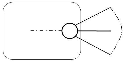
(f) 6

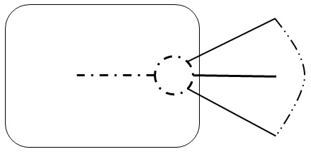
(g) 7

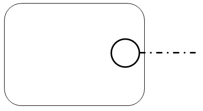
(h) 8

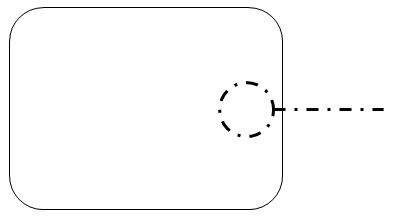
(i) 9

Figure 3: Different cases for a vertex $v\in X_{i}$ in correspondence to the edges and vertices in $X_{i}$.

For each edge, there are three different possible cases to consider: (1) it is in the mixed dominating set, (2) it is not in the mixed dominating set and it is covered by some element(s), or (3) it is not in the mixed dominating set and is not covered by any element. These cases are summarized in Table 3.

Table 3: Possible condition for an edge.

1	edge belongs to the mixed dominating set.
2	edge does not belong to mixed dominating set, but it is covered
3	edge is not in mixed dominating set and also is not covered.

For our algorithm, we keep two types of data tables: (1) The bag table $Btable_{i}$ saves all of the possible states for the vertices and the edges in the bag $X_{i}$. (2) The status table $Stable_{i}$ saves all possible states for the vertices and the edges in the bag $X_{i}$ with respect to $G_{i}^{\triangle}$. Each table is constructed as follows: in both $Btable_{i}$ and $Stable_{i}$ each row represents a possible solution and each column corresponds to a vertex or an edge in the induced graph $X_{i}$. In addition they both have a column with a cost value that shows the number of mixed domination members in that row. The ordering of cells in each row of these tables is $v_{0},\;...,\;v_{w},\;e_{1},\;...,\;e_{\binom{w+1}{2}},\;cost$.

4 Our Proposed Algorithm

In this section, we present our proposal algorithm to find the mixed domination number for a graph with bounded tree-width. This algorithm consists of three phases:

• Let $G=(V,E)$ be an unweighted and undirected graph with constant tree-width. We compute and then use a standard very nice tree decomposition with width $w$. It can be done in time $O(n)$ using Lemma 2.3.

• We find a postorder traversal $\tau$ on the very nice tree decomposition. The traversal $\tau$ begins from the leftmost leaf and then goes up in the tree until it reaches the first join bag. Then, it goes to the leftmost leaf on the right subtree of the join bag recursively. It goes up if both children of the join bag are visited and visits the join bag itself and continues until it reaches the root. This phase can be computed in $O(n)$ time.

• We follow elements of $\tau$ in order and update the corresponding tables for each bag as follows:

  • Whenever we reach a leaf bag, we create a new table which contains all of the possible cases that the bag can be in.

  • Whenever we reach an introduce bag, we construct a new table for the bag from its child table.

  • Whenever we reach a join bag, we construct a new table for the bag from its children tables.

  • Whenever we reach a forget bag, we construct the table to obtain all of the possible states that vertices in this bag can have by considering edges and vertices which appeared heretofore.

  It is clear that the time complexity of this phase relates to the time spent in processing each bag in the traversal $\tau$. This process includes time to create a table for each leaf bag and time to combine two tables for the introduce, the forget and the join bags. A new table is created with two rows, running in constant time, therefore these operations add a constant time factor. To combine two tables we consider the worst case. The table for a join or an introduce bag can be created in $O(w^{2})$ steps and for a forget bag requires $O(w)$ steps. The worst case for join bag happens when they have all possible cases which lead to $9^{w+1}\times 3^{\binom{w+1}{2}}$ rows. Therefore, the time complexity of this phase equals $O(9^{w}\times 3^{w^{2}}\times w^{2})$.

The algorithm described so far is polynomial-time with respect to the size of $T$, Lemma 2.3 shows this size is $O(n)$. However, it is exponential with respect to the tree-width of $T$, $w$. The following theorem states the time complexity of our proposed algorithm.

Theorem 4.1.

The running time of the described approach is $O(9^{w}\times 3^{w^{2}}\times w^{2}\times n)$.

Our proposed dynamic programming algorithm works on $\tau$ which is the postorder traversal on a very nice tree decomposition of $G$. When the algorithm visits a bag, it describes the partial solutions to AMDS and as it continues to other bags, it extends the created partial solutions. These partial solutions need to satisfy all of the problem specific constraints in $G_{i}^{\triangle}$ except for the vertices in $X_{i}$ and their incident edges in $G_{i}^{\triangle}\backslash G_{i}$. The status tables $Stable$ are used to store these partial solutions. In other words, a $Stable$ characterizes the partial solutions and each row in $Stable$ contains a valid assignment for vertices and edges in $G_{i}$.

To compute the $Stable$ of each bag $i$, our algorithm uses $Btable$ of the children of bag $i$. Since these tables are computed bottom-up, the final solution of the MDS appears in the root of $T$. So, it can be extracted by inspecting the table of the root. The Algorithm 1 demonstrates how we achieve the final answer $\gamma_{md}$.

Algorithm 1 The algorithm to compute $\gamma_{md}$.

INPUT: Postorder traversal $\tau$ on a standard very nice tree decomposition of graph $G$.

OUTPUT: $\gamma_{md}$ for $G$.

for $i\leftarrow 1$ to $|\tau|$ do

     if  $X_{i}$ is a bag leaf then

         Create a new table with two rows each corresponding to cases 2 and 5 for the isolated vertex in $X_{i}$ (see Section 4.1) .

     else if  $X_{i}$ is an introduce bag then

         for $\ell_{1}\leftarrow 1$ to number of rows in $Stable_{i-1}$ do

              for $\ell_{2}\leftarrow 1$ to number of rows in $Btable_{i}$ do

                  Call Algorithm 2 with inputs $r_{Stable_{i-1}}(\ell_{1},:)$ and $r_{Btable_{i}}(\ell_{2},:)$.

              end for

         end for

     else if  $X_{i}$ is a forget bag  then

         for $\ell_{1}\leftarrow 1$ to number of rows in $Stable_{i-1}$ do

              Call Algorithm 3 with input $r_{Stable_{i-1}}(\ell_{1},:)$.

         end for

     else if  $X_{i}$ is a join bag  then

         for $\ell_{1}\leftarrow 1$ to number of rows in $Stable_{i1}$ do

              for $\ell_{2}\leftarrow 1$ to number of rows in $Stable_{i2}$ do

                  Call Algorithm 4 with inputs $r_{Stable_{i1}}(\ell_{1},:)$ and $r_{Stable_{i2}}(\ell_{2},:)$.

              end for

         end for

     end if

     Add the created rows to $Stable_{i}$.

end for

When Algorithm 1 observes a leaf bag, it creates a new table which saves all of the possible states for the only vertex in that bag. The algorithm when following the traversal $\tau$ calls Algorithms 2, 3 and 4 when observing introduce, forget and join bags respectively, and return $\gamma_{md}$ as output. Note that it is possible that combining two rows in different levels may create the same rows. In this case we store the row with minimum cost in $Stable_{i}$. To avoid searching and sorting to find these repeated states, we use a coding to store the created rows. We use a help table in which each created row has a specific position in it. When a row is created while combining two tables, the help table is checked and if there is a row with lower cost, then the lower cost is considered and the help table is updated accordingly. Finally Algorithm 1 inspects the root table and finds $\gamma_{md}$. For illustration, we consider the graph in Figure 1(a) and one of its nice tree decomposition (see Figure 1(b)) as an example for our proposed algorithm. The output of the algorithm is $\gamma_{md}=2$. Next, we describe how the tables are filled and partial solutions are computed.

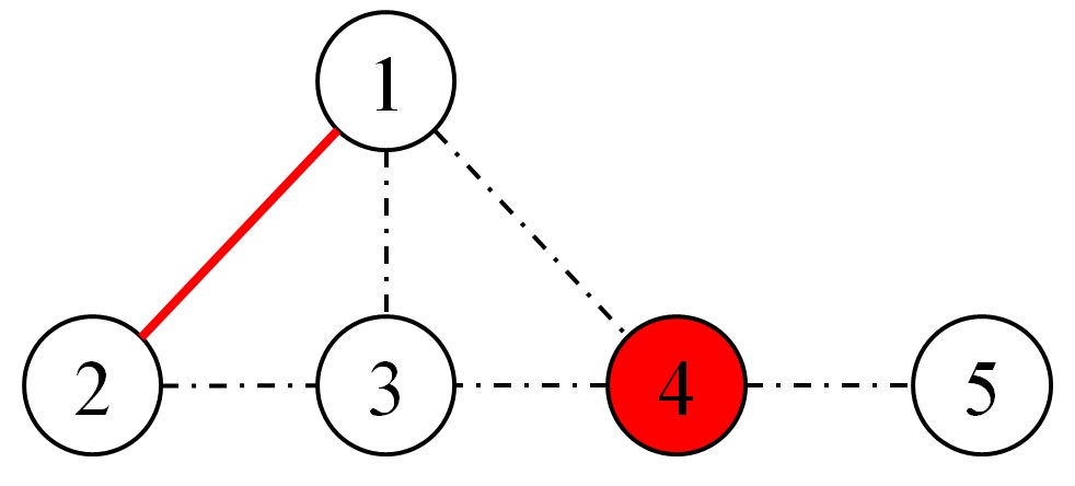
Figure 4: Mixed domination of the graph $G1$.

4.1 Status table construction for leaf bags

During the traversal $\tau$, when we observe a leaf bag, a new table is created which saves all of the possible states for the only vertex in that bag. Let $X_{i}$ be a leaf bag since we are working with a standard nice tree decomposition, every leaf bag contains exactly one vertex. For vertex $v\in X_{i}$, the status table $i$ denoted as $Stable_{i}$ contains two rows. The first row corresponds to the situation in with vertex $v$ belongs to an optimal mixed domination set, and the last one is for the case in which vertex $v$ does not belong to an optimal mixed domination set. Therefore, this table has two rows wherein the first row, the value of the vertex is $``2"$ by costing $``1"$, and in the second row, the value of the vertex is $``5"$ by costing $``0"$. The status table of leaf bag 1 in Figure 1(b) is shown in Table 4.

Table 4: The status table of leaf bag 1 in Figure 1(b).

	vertices			edges
case	2	-	-	-	-	-	cost
1	2	0	0	0	0	0	1
2	5	0	0	0	0	0	0

4.2 Construction of the status table for an introduce bag

An introduce bag $X_{i}$ has one more vertex than its child bag $X_{i-1}$ as well as the edges that are adjacent to the new vertex and the vertices of the previous bag. Assume $Stable_{i-1}$ contains all of the possible states that can occur up to this level for visited edges and vertices. After adding the new vertex and the corresponding edges we need to add all of the new possible states to the new $Stable_{i}$. To do so, we compute $Stable_{i}$ as $Stable_{i-1}\otimes Btable_{i}$. Assume that $n$ is the size of bag $X_{i}$, $e$ is the number of edges with both ends in $X_{i}$, $r_{Stable_{i-1}}(\ell_{1},:)$ and $r_{Btable_{i}}(\ell_{2},:)$ are two rows of $Stable_{i-1}$ and $Btable_{i}$, and $j$ refers to the entries of a row of a table. Then, Equation 2 describes the construction of the entries of $\ell$th row of $Stable_{i}$.

$$r_{Stable_{i}}(\ell,j)=\begin{cases}r_{Stable_{i-1}}(\ell_{1},j)\star_{Int}r_{Btable_{i}}(\ell_{2},j),&\text{if $0\leq j\leq w$ },\\ r_{Stable_{i-1}}(\ell_{1},j)\ast_{Int}r_{Btable_{i}}(\ell_{2},j),&\text{if $w+1\leq j\leq w+\binom{w+1}{2}$ },\\ r_{Stable_{i-1}}(\ell_{1},j)$ + $r_{Btable_{i}}(\ell_{2},j)$ - $|A|$ - $|B|,&\text{if $j=w+\binom{w+1}{2}+1$ },\\ \end{cases}$$ (2)

where

$$A=\{\alpha\mid(r_{Stable_{i-1}}(\ell_{1},\alpha)\leq 2\wedge\hskip 3.0ptr_{Btable_{i}}(\ell_{2},\alpha)\leq 2)\wedge(0\leq\alpha\leq w)\},$$ (3)

$$B=\left\{\alpha\mid\left(r_{Stable_{i-1}}(\ell_{1},\alpha)=1\wedge\hskip 3.0ptr_{Btable_{i}}(\ell_{2},\alpha)=1)\wedge(w+1\leq\alpha\leq w+{\textstyle\binom{w+1}{2}}\right)\right\}.$$ (4)

In Equation 2, two multiplication operators $\star_{Int}$ and $\ast_{Int}$ are used to compute the entries of $Stable_{i}$. The multiplication tables for these operators are given in Tables 5 and 6. Note that value $``-"$   in Tables 5, 6, 12 and 13 never happen. The Algorithm 2 describes aforementioned approach in constructing rows of $Stable_{i}$ in a formal manner. Algorithms 2, 3 and 4 calculate the value of $\ell$ using Equation 5. After constructing an entire row in $Stable_{i}$, the value of $\ell$ is obtained as follows: Assume that $(r_{0},r_{1},...,r_{w},r_{w+1},...,r_{w+\binom{w+1}{2}},r_{w+\binom{w+1}{2}+1})$ is the output of the algorithms, then number $\ell$ shows the number of a row that this output is saved in it. Equation 5 shows how the value of $\ell$ is calculated. Array $r_{HP}$ is used to save entries of a row until the value of $\ell$ is computed. If the $\ell$th row in $Stable_{i}$ is empty, the algorithm saves the output. However if the $\ell$th row was filled, and if the new $r_{w+\binom{w+1}{2}+1}$ is less than the existing one, the algorithm replaces the value of $r_{w+\binom{w+1}{2}+1}$.

$$\ell=\left(\sum_{i=0}^{w}r_{i}\times 9^{i}\right)+\left(\left(\sum_{j=1}^{\binom{w+1}{2}}r_{w+j}\times 4^{j-1}\right)\times 9^{w+1}\right).$$ (5)

Table 5: Multiplication operation for vertices in introduce bag.

$\star_{Int}$	0	1	2	3	4	5	6	7	8	9
0	0	-	-	-	-	-	-	-	-	-
1	1	1	1	1	1	1	1	1	1	1
2	2	1	2	1	2	2	2	2	2	2
3	3	1	1	3	3	3	3	3	3	3
4	4	1	2	3	4	4	4	4	8	8
5	4,5	1	2	3	4	5	4	5	8	9
6	4,6	1	2	3	4,6	4,6	4,6	4,6	8	8
7	4,5,6,7	1	2	3	4,6	5,7	4,6	5,7	8	9

Table 6: Multiplication operation for edges in introduce bag.

$\ast_{Int}$	0	1	2	3
0	0	-	-	-
1	1	1	1	1
2	2	1	2	2
3	2,3	1	2	3

The Algorithm 2 takes a row from $Stable_{i-1}$ and a row from $Btable_{i}$, and uses Equation 5 to fill elements $r_{0},...,r_{w}$ of $Stable_{i}$. Given that some of the cells in Table 5 have two values, the exact amount is determined according to the value of an adjacent edge. Algorithm 2 at first determines elements $r_{0},...,r_{w}$ of $Stable_{i}$ if the cell in Table 12 has one value. Similarly, it uses Equation 6 to fill elements $r_{w+1},...,r_{w+\binom{w+1}{2}}$ of $Stable_{i}$. Then it assigns $r_{0},...,r_{w}$ which the cell in Table 5 has two values, it chooses one of them according to the value of the adjacent edges of a vertex in bag $X_{i}$. The value of the $r_{w+\binom{w+1}{2}+1}$ is computed during the assignment of the elements $r_{0},...,r_{w+\binom{w+1}{2}}$. Computing $Stable_{2}$ as $Stable_{1}\otimes Btable_{2}$ is shown in Table 9. Algorithm 2 computes $r_{Stable_{1}}(4,:)\otimes r_{Btable_{2}}(1,:)$ as follows:

• $(\underline{2},0,0,0,0,0,1)\star_{Int}(\underline{3},3,0,1,0,0,1)\rightarrow(\underline{1},0,0,0,0,0,0)$

• $(2,\underline{0},0,0,0,0,1)\star_{Int}(3,\underline{3},0,1,0,0,1)\rightarrow(1,\underline{3},0,0,0,0,0)$

• $(2,0,0,\underline{0},0,0,1)\ast_{Int}(3,3,0,\underline{1},0,0,1)\rightarrow(1,3,0,\underline{1},0,0,0)$

• $(2,0,0,0,0,0,\underline{1})\times(3,3,0,1,0,0,\underline{1})\rightarrow(1,3,0,1,0,0,\underline{2})$

Also it computes $r_{Stable_{1}}(8,:)\otimes r_{Btable_{2}}(2,:)$ as follows:

• $(\underline{5},0,0,0,0,0,0)\star_{Int}(\underline{7},7,0,3,0,0,0)\rightarrow(\underline{?},0,0,0,0,0,0)$

• $(5,\underline{0},0,0,0,0,0)\star_{Int}(7,\underline{7},0,3,0,0,0)\rightarrow(?,\underline{?},0,0,0,0,0)$

• $(5,0,0,\underline{0},0,0,0)\ast_{Int}(7,7,0,\underline{3},0,0,0)\rightarrow(?,?,0,\underline{3},0,0,0)$

• $(\underline{5},0,0,0,0,0,0)\star_{Int}(\underline{7},7,0,3,0,0,0)\rightarrow(\underline{7},0,0,3,0,0,0)$

• $(5,\underline{0},0,0,0,0,0)\star_{Int}(7,\underline{7},0,3,0,0,0)\rightarrow(7,\underline{7},0,3,0,0,0)$

• $(5,0,0,0,0,0,\underline{0})\times(7,7,0,3,0,0,\underline{0})\rightarrow(7,7,0,,0,0,\underline{0})$

Table 7: $Stable_{1}$

	vertices			edges
case	2	-	-	-	-	-	cost
1	2	0	0	0	0	0	1
2	5	0	0	0	0	0	0

Table 8: $Btable_{2}$

	vertices			edges
case	2	3	-	4	-	-	cost
1	1	1	0	1	0	0	3
2	1	3	0	1	0	0	2
3	3	1	0	1	0	0	2
4	3	3	0	1	0	0	1
5	2	2	0	2	0	0	2
6	2	4	0	2	0	0	1
7	4	2	0	2	0	0	1
8	7	7	0	3	0	0	0

Table 9: $Stable_{2}$

	vertices			edges
case	2	3	-	4	-	-	cost
1	1	1	0	1	0	0	3
2	1	3	0	1	0	0	2
3	3	1	0	1	0	0	2
4	3	3	0	1	0	0	1
5	2	2	0	2	0	0	2
6	2	4	0	2	0	0	1
7	4	2	0	2	0	0	1
8	7	7	0	3	0	0	0

Algorithm 2 Status table’s row construction algorithm for an introduce bag.

INPUT: $r_{Stable_{i-1}}(\ell_{1},:)$ and $r_{Btable_{i}}(\ell_{2},:)$

OUTPUT: $r_{Stable_{i}}(\ell,:)$

$c\leftarrow 0$

for $j\leftarrow 0$ to $w$ do

     if $(r_{Stable_{i-1}}(\ell_{1},j)\leq 2)\textbf{ and }(r_{Btable_{i}}(\ell_{2},j)\leq 2)$ then

         $c\leftarrow c+1$

     end if

     if $|r_{Stable_{i-1}}(\ell_{1},j)\star_{Int}r_{Btable_{i}}(\ell_{2},j)|=1$ then

         $r_{HS}(1,j)\leftarrow r_{Stable_{i-1}}(\ell_{1},j)\star_{int}r_{Btable_{i}}(\ell_{2},j)$

     end if

end for

for $j\leftarrow w+1$ to $w+\binom{w+1}{2}$ do

     if $(r_{Stable_{i-1}}(\ell_{1},j)=1)\textbf{ and }(r_{Btable_{i}}(\ell_{2},j)=1)$ then

         $c\leftarrow c+1$

     end if

     if $|r_{Stable_{i-1}}(\ell_{1},j)\ast_{Int}r_{Btable_{i}}(\ell_{2},j)|=1$ then

         $r_{HS}(1,j)\leftarrow r_{Stable_{i-1}}(\ell_{1},j)\ast_{Int}r_{Btable_{i}}(\ell_{2},j)$

     else

         if  for $e_{j}=v_{r}v_{new},Stable_{i-1}(\ell_{1},r)\leq 3$ then

              $r_{HS}(1,j)\leftarrow 2$

         else

              $r_{HS}(1,j)\leftarrow 3$

         end if

     end if

end for

for $j\leftarrow 0$ to $w$ do

     if $|r_{Stable_{i-1}}(\ell_{1},j)\star_{Int}r_{Btable_{i}}(\ell_{2},j)|=2$ then

         if $r_{Stable_{i-1}}(\ell_{1},j)=0\textbf{ and }r_{Btable_{i}}(\ell_{2},j)=5$ then

              if $\exists_{w_{r}\in N^{md}_{Bag}(v_{j})},r_{HS}(1,r)\leq 2$ then

                  $r_{HS}(1,j)\leftarrow 4$

              else

                  $r_{HS}(1,j)\leftarrow 5$

              end if

         else

              if $\forall_{w_{r}\in N^{md}_{Bag}(v_{j}),e_{s}=(w_{r}v_{j})},r_{Stable_{i}}(s)\leq 2$ then

                  $r_{HS}(1,j)\leftarrow\text{first element of }r_{Stable_{i-1}}(\ell_{1},j)\ast_{Int}r_{Btable_{i}}(\ell_{2},j)$

              else

                  $r_{HS}(1,j)\leftarrow\text{second element of }r_{Stable_{i-1}}(\ell_{1},j)\ast_{Int}r_{Btable_{i}}(\ell_{2},j)$

              end if

         end if

     else

         if $\forall_{w_{r}\in N^{md}_{Bag}(v_{j}),e_{s}=(w_{r}v_{j})},r_{HS}(1,s)\leq 2\text{\bf{ and }}\exists_{w_{r}\in N^{md}_{Bag}(v_{j})},r_{HS}(1,r)\leq 2$ then

              $r_{HS}(1,j)\leftarrow 4$

         else if $\forall_{w_{r}\in N^{md}_{Bag}(v_{j}),e_{s}=(w_{r}v_{j})},r_{HS}(1,s)\leq 2\text{\bf{ and }}\forall_{w_{r}\in N^{md}_{Bag}(v_{j})},r_{HS}(1,r)\geq 3$ then

              $r_{HS}(1,j)\leftarrow 5$

         else if $\exists_{w_{r}\in N^{md}_{Bag}(v_{j}),e_{s}=(w_{r}v_{j})},r_{HS}(1,s)=3\text{\bf{ and }}\exists_{w_{r}\in N^{md}_{Bag}(v_{j})},r_{HS}(1,r)\leq 2$ then

              $r_{HS}(1,j)\leftarrow 6$

         else if $\exists_{w_{r}\in N^{md}_{Bag}(v_{j}),e_{s}=(w_{r}v_{j})},r_{HS}(1,s)=3\text{\bf{ and }}\forall_{w_{r}\in N^{md}_{Bag}(v_{j})},r_{HS}(1,r)\geq 3$ then

              $r_{HS}(1,j)\leftarrow 7$

         end if

     end if

end for

Calculate the value of $\ell$

$r_{Stable_{i}}(\ell,1:end-1)\leftarrow r_{HS}(1,1:end-1)$

if $r_{Stable_{i}}(\ell,end)>(r_{Stable_{i-1}}(\ell_{1},end)+r_{Btable_{i}}(\ell_{2},end)-c)$ then

     $r_{Stable_{i}}(\ell,end)\leftarrow r_{Stable_{i-1}}(\ell_{1},end)+r_{Btable_{i}}(\ell_{2},end)-c$

end if

4.3 Construction of the status table for a forget bag

A forget bag $X_{i}$ loses one vertex and its incident edges with respect to its present bag $X_{i-1}$. So, it is enough to omit the invalid rows from $Stable_{i-1}$ to obtain the $Stable_{i}$ for bag $X_{i}$. Algorithm 3 describes an approach for constructing rows of $Stable_{i}$. This algorithm takes a row from $Stable_{i-1}$. Let vertex $v_{eliminated}$ is the vertex that will be deleted in bag $X_{i}$. If this vertex has values 5, 7, 8 and 9, the algorithm omits this row, but if it has value 6, the algorithm updates the value of $N(v)$ in bag $X_{i-1}$. When its neighbor is covered but the edge between them is not covered, the neighbor’s value changes to 8, and when none of its neighbors and edges between them are not covered, the neighbor’s value changes to 9. For example Algorithm 3 takes rows of $Stable_{11}$ and constructs $Stable_{12}$.

Table 10: $Stable_{11}$

	vertices			edges
case	1	4	-	3	-	-	cost
1	1	1	0	1	0	0	4
2	1	2	0	2	0	0	3
3	1	3	0	1	0	0	4
4	1	3	0	2	0	0	3
5	1	4	0	2	0	0	3
6	1	8	0	2	0	0	3
7	2	1	0	2	0	0	3
8	2	2	0	2	0	0	3
9	2	3	0	2	0	0	3
10	2	4	0	2	0	0	3
11	2	8	0	2	0	0	3
12	3	1	0	1	0	0	3
13	3	1	0	2	0	0	3
14	3	2	0	2	0	0	2
15	3	3	0	1	0	0	3
16	3	3	0	2	0	0	3
17	3	4	0	2	0	0	3
18	3	8	0	2	0	0	3
19	4	1	0	2	0	0	3
20	4	2	0	2	0	0	2
21	4	3	0	2	0	0	3
22	5	3	0	2	0	0	2
23	6	6	0	3	0	0	3
24	7	6	0	3	0	0	2
25	7	7	0	3	0	0	1
26	8	1	0	2	0	0	3
27	8	2	0	2	0	0	2
28	8	3	0	2	0	0	2
29	8	6	0	3	0	0	2
30	8	8	0	2	0	0	2

Table 11: $Stable_{12}$

	vertices			edges
case	1	-	-	-	-	-	cost
1	1	0	0	0	0	0	3
2	2	0	0	0	0	0	3
1	3	0	0	0	0	0	2
2	4	0	0	0	0	0	2
1	5	0	0	0	0	0	2
2	8	0	0	0	0	0	2

Algorithm 3 Status table’s row construction algorithm for a forget bag.

INPUT: $r_{Stable_{i-1}}(\ell,:)$

OUTPUT: $r_{Stable_{i}}(\ell,:)$ or 0

if $(r_{Stable_{i-1}}(\ell,v_{eliminated})\geq 7)$ or $(r_{Stable_{i-1}}(\ell,v_{eliminated})=5)$ then

     Return 0

else

     $r_{HS}(1,:)\leftarrow r_{Stable_{i-1}}(\ell,:)$

     if $r_{Stable_{i-1}}(\ell,v_{eliminated})=6$ then

         if $(\forall_{v_{r}\in N^{md}_{X_{i-1}}(v_{eliminated}),e_{s}=(v_{r},v_{eliminated})},r_{Stable_{i-1}}(\ell,r)=6)\text{\bf{ and }}(r_{Stable_{i-1}}(\ell,s)=3)$ then

              $r_{HS}(\ell,r)\leftarrow 8$

         else if $(\forall_{v_{r}\in N^{md}_{Bag_{i-1}}(v_{eliminated}),e_{s}=(v_{r},v_{eliminated})},r_{Stable_{i-1}}(\ell,r)=7)\text{\bf{ and }}(r_{Stable_{i-1}}(\ell,s)=3)$ then

              $r_{HS}(\ell,r)\leftarrow 9$

         end if

     end if

end if

Calculate the value of $\ell$

$r_{Stable_{i}}(\ell,:)\leftarrow r_{HS}(1,:)$

$r_{HS}(\ell,v_{eliminated})\leftarrow 0$

$\forall_{v_{r}\in N^{md}_{X_{i-1}}(v_{eliminated}),e_{s}=(v_{r},v_{eliminated})},r_{HS}(\ell,s)\leftarrow 0$

4.4 Construction of the status table for a join bag

A join bag $X_{i}$ has the same set of vertices and edges with its two children ${X_{i1}}$ and ${X_{i2}}$. To construct possible states for $X_{i}$ in $Stable_{i}$, we compute $Stable_{i}=Stable_{i1}\otimes Stable_{i2}$. Let $r_{Stable_{i1}}(\ell_{1},:)$ and $r_{Stable_{i2}}(\ell_{2},:)$ be two rows of $Stable_{i1}$ and $Stable_{i2}$, and $j$ refers to the entries of a row of a table. Equation 2 describes how to construct the rows of $Stable_{i}$.

$$r_{Stable_{i}}(\ell,j)=\begin{cases}r_{Stable_{i1}}(\ell_{1},j)\star_{Join}r_{Stable_{i2}}(\ell_{2},j),&\text{if $0\leq j\leq w$ }.\\ r_{Stable_{i1}}(\ell_{1},j)\ast_{Join}r_{Stable_{i2}}(\ell_{2},j),&\text{if $w+1\leq i\leq w+\binom{w+1}{2}$ }.\\ r_{Stable_{i1}}(\ell_{1},j)$ + $r_{Stable_{i2}}(\ell_{2},j)$ - $|A|$ - $|B|,&\text{if $i=w+\binom{w+1}{2}+1$ }.\\ \end{cases}$$ (6)

where

$$A=\left\{\alpha\mid(r_{Stable_{i1}}(\ell_{1},\alpha)\leq 2\wedge\hskip 3.0ptr_{Stable_{i2}}(\ell_{2},\alpha)\leq 2)\wedge(0\leq\alpha\leq w)\right\}.$$ (7)

$$B=\left\{\alpha\mid\left(r_{Stable_{i1}}(\ell_{1},\alpha)=1\wedge\hskip 3.0ptr_{Stable_{i2}}(\ell_{2},\alpha)=1)\wedge(w+1\leq\alpha\leq w+1+{\textstyle\binom{w+1}{2}}\right)\right\}.$$ (8)

In Equation 6, two different multiplication operations $\star_{Join}$ and $\ast_{Join}$ are used to obtain the entries of $Stable_{i}$. Their multiplication tables are given in Tables 12 and 13. Algorithm 4 describes how to construct the rows of $Stable_{i}$ precisely. Given that some of the cells in Table 12 have two values we do as before. Algorithm 4 at first determines elements $r_{0},...,r_{w}$ of $Stable_{i}$ if the cell in Table 12 has one value then it uses Table 13 to fill elements $r_{w+1},...,r_{w+\binom{w+1}{2}}$ of $Stable_{i}$. Finally, it assigns $r_{0},...,r_{w}$ when the cell in Table 12 has two values, it chooses one as mentioned before. The value of $r_{w+\binom{w+1}{2}+1}$ that is computed during the assignment of the elements is $r_{0},...,r_{w+\binom{w+1}{2}}$.

Table 12: Multiplication operation for vertices in join bag.

$\star_{Join}$	0	1	2	3	4	5	6	7	8	9
0	0	-	-	-	-	-	-	-	-	-
1	-	1	1	1	1	1	1	1	1	1
2	-	1	2	1	2	2	2	2	2	2
3	-	1	1	3	3	3	3	3	3	3
4	-	1	2	3	4	4	4	4	8	8
5	-	1	2	3	4	5	4	5	8	9
6	-	1	2	3	4	4	First Second 4 6	First Second 4 6	8	8
7	-	1	2	3	4	5	First Second 4 6	First Second 5 7	8	9
8	-	1	2	3	8	8	8	8	8	8
9	-	1	2	3	8	9	8	9	8	9

Table 13: Multiplication operation for edges in join bag.

$\ast_{Join}$	0	1	2	3
0	0	-	-	-
1	-	1	1	1
2	-	1	2	2
3	-	1	2	3

Algorithm 4 computes $Stable_{1}\otimes Btable_{2}$ to construct $Stable_{2}$. The status table of bag 12 of Figure 1(b) is shown in Table 16.

Table 14: $Stable_{6}$

	vertices			edges
case	1	4	-	3	-	-	cost
1	1	1	0	1	0	0	4
2	1	2	0	2	0	0	3
3	1	3	0	1	0	0	3
4	1	3	0	2	0	0	2
5	1	4	0	2	0	0	2
6	1	8	0	2	0	0	2
7	2	2	0	2	0	0	3
8	2	4	0	2	0	0	2
9	2	8	0	2	0	0	2
10	3	1	0	1	0	0	3
11	3	1	0	2	0	0	3
12	3	2	0	2	0	0	2
13	3	3	0	1	0	0	2
14	3	3	0	2	0	0	2
15	3	4	0	2	0	0	2
16	3	5	0	2	0	0	2
17	3	9	0	2	0	0	2
18	4	1	0	2	0	0	2
19	4	2	0	2	0	0	2
20	4	3	0	2	0	0	2
21	5	3	0	2	0	0	2
22	6	6	0	3	0	0	2
23	6	7	0	3	0	0	2
24	7	7	0	3	0	0	1
25	8	1	0	2	0	0	3
26	8	2	0	2	0	0	2
27	8	3	0	2	0	0	2
28	8	6	0	3	0	0	1
29	8	9	0	3	0	0	1

Table 15: $Stable_{10}$

	vertices			edges
case	1	4	-	3	-	-	cost
1	1	1	0	1	0	0	3
2	1	3	0	1	0	0	3
3	2	2	0	2	0	0	2
4	2	3	0	2	0	0	2
5	2	4	0	2	0	0	2
6	2	3	0	2	0	0	2
7	3	1	0	1	0	0	2
8	3	3	0	1	0	0	2
9	4	1	0	2	0	0	2
10	4	2	0	2	0	0	1
11	5	3	0	2	0	0	1
12	7	6	0	3	0	0	1

Table 16: $Stable_{11}$

	vertices			edges
case	1	4	-	3	-	-	cost
1	1	1	0	1	0	0	4
2	1	2	0	2	0	0	3
3	1	3	0	1	0	0	4
4	1	3	0	2	0	0	3
5	1	4	0	2	0	0	3
6	1	8	0	2	0	0	3
7	2	1	0	2	0	0	3
8	2	2	0	2	0	0	3
9	2	3	0	2	0	0	3
10	2	4	0	2	0	0	3
11	2	8	0	2	0	0	3
12	3	1	0	1	0	0	3
13	3	1	0	2	0	0	3
14	3	2	0	2	0	0	2
15	3	3	0	1	0	0	3
16	3	3	0	2	0	0	3
17	3	4	0	2	0	0	3
18	3	8	0	2	0	0	3
19	4	1	0	2	0	0	3
20	4	2	0	2	0	0	2
21	4	3	0	2	0	0	3
22	5	3	0	2	0	0	2
23	6	6	0	3	0	0	3
24	7	6	0	3	0	0	2
25	7	7	0	3	0	0	1
26	8	1	0	2	0	0	3
27	8	2	0	2	0	0	2
28	8	3	0	2	0	0	2
29	8	6	0	3	0	0	2
30	8	8	0	2	0	0	2

Algorithm 4 Status table’s row construction algorithm for a join bag.

INPUT: $r_{Stable_{i1}}(\ell_{1},:)$ and $r_{Stable_{i2}}(\ell_{2},:)$

OUTPUT: $r_{Stable_{i}}(\ell,:)$

for $j\leftarrow 0$ to $w$ do

     if $|r_{Stable_{i1}}(\ell_{1},j)\star_{Join}r_{Stable_{i2}}(\ell_{2},j)|=1$ then

         $r_{HS}(1,j)\leftarrow r_{Stable_{i1}}(\ell_{1},j)\star_{Join}r_{Stable_{i2}}(\ell_{2},j)$

     end if

     if $(r_{Stable_{i1}}(\ell_{1},j)\leq 2)\textbf{ and }(r_{Stable_{i}}(\ell_{2},j)\leq 2)$ then

         $c\leftarrow c+1$

     end if

end for

for $j\leftarrow w$ to $w+\binom{w+1}{2}$ do

     $r_{HS}(1,j)\leftarrow r_{Stable_{i1}}(\ell_{1},j)\ast_{Join}r_{Stable_{i2}}(\ell_{2},j)$

     if $(r_{Stable_{i-1}}(\ell_{1},j)=1)\textbf{ and }(r_{Stable_{i}}(\ell_{2},j)=1)$ then

         $c\leftarrow c+1$

     end if

end for

for $j\leftarrow 0$ to $w$ do

     if $|r_{Stable_{i1}}(\ell_{1},j)\star_{Join}r_{Stable_{i2}}(\ell_{2},j)|=2$ then

         if $\forall_{w_{r}\in N^{md}_{Bag}(v_{j}),e_{s}=(w_{r}v_{j})},r_{HS}(1,s)\leq 2$ then

              $r_{HS}(\ell,j)\leftarrow\text{First element of }r_{Stable_{i1}}(\ell_{1},j)\ast_{Join}r_{Stable_{i2}}(\ell_{2},j)$

         else

              $r_{HS}(1,j)\leftarrow\text{Second element of }r_{Stable_{i1}}(\ell_{1},j)\ast_{Join}r_{Stable_{i2}}(\ell_{2},j)$

         end if

     end if

end for

Calculate the value of $\ell$

$r_{Stable_{i}}(\ell,1:end-1)\leftarrow r_{HS}(1,1:end-1)$

if $r_{Stable_{i}}(\ell,end)>(r_{Stable_{i-1}}(end)+r_{Btable_{i}}(end)-c)$ then

     $r_{Stable_{i}}(end)\leftarrow r_{Stable_{i-1}}(end)+r_{Btable_{i}}(end)-c$

end if

Note that Algorithm 1 computes the value of $\gamma_{md}$, however it is not a minimum mixed dominating set. It is possible to modify the algorithm to obtain a mixed dominating set with minimum size. This modification is as follows. We first consider some fixed arbitrary one-to-one total numbering function $\phi$ used to code elements of $S\subseteq V\cup E$. Let $|V|=n$ and $|E|=m$, $\phi:\{V\cup E\}\xrightarrow{1-1}\{1,2,...,n+m\}$. The function $\phi$ determines an arbitrary order on set $\{V\cup E\}$. We get elements in a particular order to code a partial solution. Indeed, we display a partial solution as a binary number, i.e. every element in $\{V\cup E\}$ can have two values of 0 or 1 where 0 indicates that the corresponding element is not present (in the mixed domination set) and 1 indicates it is present. We use a function $\psi:\phi(x)\rightarrow\{0,1\}$. to convert a partial solution $x$ to a binary number. Its enough to change the algorithm and save elements of the partial solution by a binary number just after constructing each state. Other changes to the algorithm are straightforward. Note that the maximum number of bits that can be changed in a state is equal to $k+\binom{k}{2}$, where $k$ is the number of vertices in a bag.

After computing $\gamma_{md}$, our proposed algorithm traverses the tree decomposition via $\tau$ recursively and identifies the edges and vertices in the mixed domination sets. Finally, the AMDS problem is solved.

4.5 The Modified Algorithm to Solve the MDS Problem

In this section, we use the notion of fast subset convolution, which was introduced by Van et al. in Van Rooij et al. (2009), to solve MDS in time $O^{*}(6^{w})$. Van et al. introduced two new techniques, the first using a variant of convolutions, and the second being a simple way of partitioned table handling, which can be used for MDS as well. They used an alternative representation to obtain an exponentially faster algorithm. In their solution for dominating set problem, each vertex can be in three states as follow:

• Vertex is in the dominating set.

• Vertex is not in the dominating set and has already been dominated.

• Vertex is not in the dominating set and has not yet been dominated.

A vertex in their alternative representation defines two basic states $1$ and $0_{?}$. The state $0_{?}$ denotes that a vertex is not in the dominating set and may or may not be dominated by the current dominating set. The transformation can be applied by the formula of $F(c)$, which represents their table for coloring $c$.

$$F(c_{1}\times{0_{?}}\times c_{2})=F(c_{1}\times{0_{0}}\times c_{2})+F(c_{1}\times{0_{1}}\times c_{2}),$$

where $c_{1}$ is a subcoloring of size $i$, and $c_{2}$ is a subcoloring of size $k-i-1$. The transformation to basic states is applicable using

$$F(c_{1}\times{0_{1}}\times c_{2})=F(c_{1}\times{0_{?}}\times c_{2})-F(c_{1}\times{0_{0}}\times c_{2}).$$

Dynamic programming algorithm over nice tree decomposition uses $O^{*}(3^{w})$ time on leaf, introduce and forget bags, however, it uses $O^{*}(4^{w})$ time on a join bag. By using the results of the convolution of Van et al., the time complexity of a join bag is improved to $O^{*}(3^{w})$.

Now, we introduce our algorithm to solve MDS. Similar to solving the AMDS, we assign a power value to the vertices and use dynamic programming. Our solution to the MDS has two differences compared with the solution to the AMDS:

• The tables $Stable$ and $Btable$ store a valid assignment for just vertices and we do not need to consume memory to store information on edges in a beg.

• A vertex $v\in X_{i}$ has six possible states based on satisfying $v\in\mathcal{MD}$ and being covered by $N^{md}_{G}[v]$. These six conditions are illustrated in Table 17.

Table 17: Possible states for each vertex with respect to a bag in tables $Stable$ and $Btable$.

	$v\in\mathcal{MD}$	$N^{e}_{X_{i}}(v)\in\mathcal{MD}$	vertex cover	edge cover	vertex power
1	$v\in\mathcal{MD}$	$\forall e\in N^{e}_{X_{i}}(v)$	$v$ is covered	$\forall e\in N^{e}_{X_{i}}(v),e$ is covered	2
3	$v\notin\mathcal{MD}$	$\exists e\in N^{e}_{X_{i}}(v),e\in\mathcal{MD}$	$v$ is covered	$\forall e\in N^{e}_{X_{i}}(v),e$ is covered	1
4	$v\notin\mathcal{MD}$	$\forall e\in N^{e}_{X_{i}}(v),e\notin\mathcal{MD}$	$v$ is covered	$\forall e\in N^{e}_{X_{i}}(v),e$ is covered	0
5	$v\notin\mathcal{MD}$	$\forall e\in N^{e}_{X_{i}}(v),e\notin\mathcal{MD}$	$v$ is not covered	$\forall e\in N^{e}_{X_{i}}(v),e$ is covered	0
6	$v\notin\mathcal{MD}$	$\forall e\in N^{e}_{X_{i}}(v),e\notin\mathcal{MD}$	$v$ is covered	$\exists e\in N^{e}_{X_{i}}(v),e$ is not covered	0
7	$v\notin\mathcal{MD}$	$\forall e\in N^{e}_{X_{i}}(v),e\notin\mathcal{MD}$	$v$ is not covered	$\exists e\in N^{e}_{X_{i}}(v),e$ is not covered	0

These six states are the same as the seven states in Section 3, except for the state 2. The state 2 is deleted since it has the same effect as state 1 on $N^{md}_{G}[v]$, since we do not store any information on edges in the tables $Stable$ and $Btable$.

We follow the three phases of our proposed algorithm in Section 4. Note the storage tables $Stable$ and $Btable$ store a valid assignment only for the vertices. During the traversal $\tau$, when we observe a leaf bag, a new table is created which saves all of the possible states for the only vertex in that bag. In an introduce or a join bag, the multiplication operators $\star_{Int}$ and $\star_{Join}$ in Equations 2 and 6, respectively, are used to compute the entries of $Stable_{i}$. This algorithm omits the invalid rows from $Stable_{i-1}$ to obtain the $Stable_{i}$ for bag $X_{i}$ in a forget bag.

It is clear that the time complexity of this algorithm relates to the time spent for processing each bag in the traversal of $\tau$. In a bag, we have at most $w+1$ vertices. So, This algorithm uses $O(6^{w})$ time on leaf, introduce and forget bags but $O(7^{w})$ time on a join bag. To reduce the time spent for a join bag, we use the fast subset convolution to multiply the two tables of size $6^{w}$ in time $O(6^{w})$. In this multiplication technique, we use the notion of fast subset convolution and convert the two tables $Stable$ and $Btable$ to two new tables $Stable^{\prime}$ and $Btable^{\prime}$. In these new tables, states $5$ and $7$ are merged to a new state $0_{?}$ where this vertex is not covered and its edges may or may not be covered. Therefore, it suffices to multiply the two tables since no states in a join bag tables are lost. Using the results of convolution and alternative representations of vertex states, our algorithm for MDS improves to $O^{*}(6^{w})$.

5 The Correctness of the Algorithms

In this section, we first show that finding the mixed domination number of graphs is checkable in linear-time if the graph has bounded tree-width using Courcelle’s Theorem Courcelle (1990). Then, we describe how to ensure that our proposed bottom-up method solves MDS by computing partial solutions as state tables for bags. A partial solution is an object which stores all possible states for vertices and edges in a bag. Therefore, what we need to show is showing that how a partial solution can be extended to a final solution.

To show that the mixed domination property of graphs can be checked in linear-time for graphs with bounded tree-width, we consider the following to express mixed domination in monadic second-order logic.

• Vertices, edges, sets of vertices and edges of a graph G as variables of monodic second order logic.

• Relations $adj(p,q)$ and $inc(p,q)$ which are defined as follows: $adj(p,q)$ is a binary adjacency relation and it is true if and only if $p$ and $q$ are two adjacent vertices or are two adjacent edges of $G$, and $inc(p,q)$ is a binary incidence relation and it is true if and only if edge $p$ is incident to vertex $q$ or vertex $p$ is incident to edge $q$.

• The set operations $\cup$, $\cap$, $\subseteq$ and $\in$ denote the union, the intersection, the subset and the membership operators, respectively.

• Unary set cardinality operator $\left|{S}\right|$ and the set equality operator $=$.

• The comparison operator $\leq$.

• The logical connectives AND $(\wedge)$ and OR $(\vee)$.

• The logical quantifiers $\forall$ and $\exists$ over vertices, edges, sets of vertices and edges of G.

By modeling the mixed domination property of graphs in the described monadic second-order logic, we can conclude that checking this property on graphs with a bounded tree-width is a linear time task. Let $G=(V,E)$ be a given simple graph. For any element $r\in V\cup E$, the mixed neighborhood of $r$ is denoted by $N^{md}(r)$ and is defined as $N^{md}_{G}(r)=\{s\in V\cup E\mid adj(s,r)\vee inc(s,r)\}$ and the closed neighborhood of $r$ is denoted by $N^{md}_{G}[r]$ and equals $N^{md}_{G}[r]=N^{md}_{G}(r)\cup\{r\}$. A subset $\mathcal{S}\subseteq V\cup E$ is a mixed dominating set (MDS) for $G$, if for all ${r\in V\cup E},$ it is the case that $|N^{md}_{G}[r]\cap\mathcal{S}|\geq 1$. The mixed domination number problem asks for the size of $S$ which is expressed as in Equation 9:

$$\exists S\subseteq(V\cup E),\;S\text{ is an MDS }\wedge\;\forall M\subseteq(V\cup E),\;M\text{ is an MDS},\;|S|\leq|M|.$$ (9)

To show the correctness of our algorithm, it is enough to show that the extension of a partial solution satisfies the condition of the restricted form of mixed domination problem. Extending a partial solution begins by constructing a table for a leaf bag. At first, the leaf table contains two possible states (see Section 4.1). Obviously, these two states are all possible states that can occur for a vertex in a bag.

According to the definition of the tree decomposition, a bag $X_{i}$ is a separator whenever it separates the vertices of $(X^{\triangle}_{i})\backslash X_{i}$ from $V\backslash(X^{\triangle}_{i})$, so the vertices of $(X^{\triangle}_{i})\backslash X_{i}$ do not appear in other bags except the ones descending from bag $X_{i}$. Hence, in our bottom-up approach, all of the possible states have been considered for vertices of bag $X_{i}$ since they will never be considered again. Using this fact, we continue the proof of correctness of our algorithm by first checking the extension of an introduce bag.

Lemma 5.1.

Let $Stable_{i-1}$ and $Btable_{i}$ be two tables with all possible states mentioned in Table 2 and Table 1 for $X_{i-1}$ and $X_{i}$ respectively. Combining these two tables according to Algorithm 1 produces all of the possible states for bag $X_{i}$.

Proof.

The proof is by contradiction. A new states state $r\in Stable_{i}$ is the result of multiplying two possible states $r_{1}\in Stable_{i-1}$ and $r_{2}\in Btable_{i}$. We need to show that state $r$ cannot be produced by impossible states. Let $r^{\prime}_{1}$ be a possible and $r^{\prime}_{2}$ be an impossible state, hence $r^{\prime}_{1}\in Stable_{i-1}$ and $r^{\prime}_{2}\notin Btable_{i}$ and $r=r_{1}\otimes r_{2}$. Since $r$ is a possible state, then it preserves all of the restrictions of MDS while state $r^{\prime}_{2}\notin Btable_{i}$ does not satisfy those restrictions and is impossible. So, because we cannot satisfy some restrictions in the entire problem while for a part of it, it is not satisfied. Similarly, the proof for cases $r^{\prime}_{1}\notin Stable_{i-1}$ and $r^{\prime}_{2}\in Btable_{i}$ or $r^{\prime}_{1}\notin Stable_{i-1}$ and $r^{\prime}_{2}\notin Btable_{i}$ is similar. Combining $Stable_{i-1}$ and $Btable_{i}$ produces all of the possible states for bag $X_{i}$. ∎

In the second step, we show how the extension of a forget bag satisfies restriction mixed domination problem. The proof is by contradiction.

Lemma 5.2.

Let $Stable_{i-1}$ be a table with all possible states for bag $X_{i-1}$. Deleting invalid rows from this table produces all of the possible states for bag $X_{i}$.

Proof.

Suppose that the vertex $v$ is the forget vertex, thus it does not appear in later steps, all of its edges have appeared up to now and all its possible states are checked before constructing $Stable_{i-1}$. For vertex $v$ and its edges, there are four cases to consider:

• vertex $v$ and its edges are dominated: In these cases, the value of vertex $v$ is either 1, 2, 3 or 4. So, they are valid cases and remain in $Stable_{i}$

• vertex $v$ is not dominated: For these cases, the value of $v$ is either 5, 7 or 9. So, they are invalid cases and are not allocated to appear in $Stable_{i}$ since no neighbor of vertex $v$ appeared till now.

• vertex $v$ is dominated but at least one of its edges in $G_{i-1}^{\triangle}\backslash G_{i-1}$ is not dominated: Let $e$ be an edge in $G_{i-1}^{\triangle}\backslash G_{i-1}$ which is not dominated. Edge $e$ causes the value of vertex $v$ to be 8 and makes invalid cases. So, these cases must be omitted from $Stable_{i}$ since edge $e$ has not any neighbor which appeared till now.

• vertex $v$ and its edges in $G_{i-1}^{\triangle}\backslash G_{i-1}$ are dominated but at least one of its edges in $G_{i-1}$ is not dominated: Let $e=(v,v^{\prime})$ be an edge in $G_{i-1}$ that is not dominated. So, edge $e$ causes the value of $v$ to be 6. By deleting vertex $v$, edge $e$ is converted to an external edge for bag $i$ and does not appear in $G_{i}$. However it is possible that an edge appears in later steps and dominates $e$, so this states can be extended to a solution and we need to save it. Thus, we consider the effect of edge $e$ on vertex $v^{\prime}$ and change the value of vertex $v^{\prime}$.

∎

In the third step, we are going to check the correctness of our algorithm in the extension of a join bag.

Lemma 5.3.

Let $Stable_{i1}$ and $Stable_{i2}$ be tables with all possible states mentioned in Table 2 and Table 1 for children of bag $X_{i}$. Combining these two tables produces all of the possible states for bag $X_{i}$.

Proof.

The proof is by contradiction and is similar to Lemma 5.1, except that $r^{\prime}_{1}\in Stable_{i1}$ and $r^{\prime}_{2}\notin Stable_{i2}$ and for other cases similarly $r^{\prime}_{1}\notin Stable_{i1}$ and $r^{\prime}_{2}\in Stable_{i2}$ and $r^{\prime}_{1}\notin Stable_{i1}$ and $r^{\prime}_{2}\notin Stable_{i2}$. ∎

Theorem 5.4.

Our proposed mixed domination algorithm produces all possible states satisfying MDS.

Proof.

A partial solution starts by considering a leaf bag and initializing the leaf table to contain all two possible states. By Lemmas 5.1, 5.2 and 5.3, we proved that every extension of partial solutions contains all of the possible states that satisfy the conditions of a mixed domination set, Thus, our algorithm produces all possible states required. ∎

Lemma 5.5.

Every extension of a partial solution preserves possible states with minimum cost.

Proof.

The Algorithm 1 stores rows of $Stable_{i}$ using a coding scheme and updates the state with minimum cost. So, every extension of a partial solution preserves possible states with minimum cost. ∎

Theorem 5.6.

Our proposed dynamic algorithm computes $\gamma_{md}$ of graphs with constant tree-width in the status table of root bag, e.g. $Stable_{root}$ in $O(9^{w}\times 3^{w^{2}}\times w^{2}\times n)$ time.

Proof.

According to the Theorem 5.4 and Lemma 5.5, our algorithm preserves possible states with minimum cost in every bag, so $Stable_{root}$ contains all of the possible states with minimum cost. To find $\gamma_{md}$, it is enough for the algorithm to find the smallest cost among all of the possible states in the root bag. Also Theorem 4.1 expresses the time complexity of this algorithm. So, the desired result is obtained. ∎

6 Conclusion

In this paper, we proposed an algorithm to solve MDS and AMDS of graphs with bounded tree-width. Our algorithm used a novel technique of inputting edge domination power to vertices of the graph. Using this technique and by analyzing our algorithm, we have shown for the first time that MDS is fixed-parameter tractable. We provided detailed dynamic program is given with running time $O^{*}(3^{w^{2}})$ and a theoretical improved version with running time $O^{*}(6^{w})$ .

As a future work, we suggest enhancing the running time of our algorithm for special classes of graphs. Studying other parameters for MDS such as path-width seems a fruitful topic, too. More importantly, exploiting our technique of assigning power values to vertices from edges to solve other graph problems is another research direction.