Two-Loop Renormalization of Quantum Gravity Simplified

Abstract

The coefficient of the dimensionally regularized two-loop $R^{3}$ divergence of (nonsupersymmetric) gravity theories has recently been shown to change when non-dynamical three forms are added to the theory, or when a pseudo-scalar is replaced by the anti-symmetric two-form field to which it is dual. This phenomenon involves evanescent operators, whose matrix elements vanish in four dimensions, including the Gauss-Bonnet operator which is also connected to the trace anomaly. On the other hand, these effects appear to have no physical consequences in renormalized scattering processes. In particular, the dependence of the two-loop four-graviton scattering amplitude on the renormalization scale is simple. In this paper, we explain this result for any minimally-coupled massless gravity theory with renormalizable matter interactions by using unitarity cuts in four dimensions and never invoking evanescent operators.

I Introduction

Recent results show that the ultraviolet structure of gravity is much more interesting and subtle than might be anticipated from standard considerations. One example of a new ultraviolet surprise is the recent identification of “enhanced ultraviolet cancellations” in certain supergravity theories N4gravThreeLoops ; N5FourLoop , which are as yet unexplained by standard symmetries KellyAttempt . Another recent example is the lack of any simple link between the coefficient of the dimensionally-regularized two-loop $R^{3}$ ultraviolet divergence of pure Einstein gravity GoroffSagnotti ; vandeVen and the renormalization-scale dependence of the renormalized theory PreviousPaper . While the value of the divergence is altered by a Hodge duality transformation that maps anti-symmetric tensor fields into scalars, the renormalization-scale dependence is unchanged. In contrast, for the textbook case of gauge theory at one loop the divergence and the renormalization-scale dependence—the beta function—are intimately linked. In Ref. PreviousPaper , a simple formula for the renormalization-scale dependence of quantum gravity at two loops was found to hold in a wide variety of gravity theories. In this paper we explain this formula via unitarity.

As established by the seminal work of ’t Hooft and Veltman HooftVeltman , pure gravity has no ultraviolet divergence at one loop. This result follows from simple counterterm considerations: after accounting for field redefinitions, the only independent potential counterterm is equivalent to the Gauss-Bonnet curvature-squared term. However, in four dimensions this term is a total derivative and integrates to zero for a topologically trivial background, so no viable counterterm remains. Hence pure graviton amplitudes are one-loop finite. Amplitudes with four or more external matter fields are, however, generally divergent.

At two loops pure gravity does diverge, as demonstrated by Goroff and Sagnotti GoroffSagnotti and confirmed by van de Ven vandeVen . The pure-gravity counterterm, denoted by $R^{3}$, is cubic in the Riemann curvature. The two-loop divergence was recently reaffirmed in pure gravity PreviousPaper , and was also studied in a variety of other theories, by evaluating the amplitude for four identical-helicity gravitons. The actual value of the dimensionally-regularized $R^{3}$ divergence changes when three-forms are added to the theory, even though they are not dynamical in four space-time dimensions. More generally, when matter is incorporated into the theory, the coefficient of the $R^{3}$ divergence changes under a Hodge duality transformation. However, such transformations appear to have no physical consequences for renormalized amplitudes PreviousPaper .

The dependence of the two-loop divergence on duality transformations is closely connected to the well-known similar dependence of the one-loop trace anomaly DuffInequivalence . One-loop subdivergences in the computation include those dictated by the Gauss-Bonnet term, whose coefficient is the trace anomaly PreviousPaper . Duff and van Nieuwenhuizen showed that the trace anomaly changes under duality transformations of $p$-form fields, suggesting that theories related through such transformations might be quantum-mechanically inequivalent DuffInequivalence . Others have argued that these effects are gauge artifacts OneLoopEquivalence ; SiegelEquivalence ; FradkinTseytlinEquivalence . For graviton scattering at two loops in dimensional regularization, quantum equivalence can be restored, but only after combining the bare amplitude and counterterm contributions PreviousPaper .

The surprising dependence of the two-loop $R^{3}$ divergence in gravity on choices of field content outside of four dimensions emphasizes the importance of focusing on the renormalization-scale dependence of renormalized amplitudes as the proper robust quantity for understanding the ultraviolet properties. The divergence itself, of course, never directly affects physical quantities since it can be absorbed into a counterterm. In contrast, the renormalization scale dependence does affect physical quantities because it controls logarithmic parts of the scaling behavior of the theory. While this is well known, what is surprising is that, in contrast to gauge theory, the two-loop divergences of pure gravity are not linked in any straightforward way to the scaling behavior of the theory. An underlying cause is that evanescent operators, such as the Gauss-Bonnet term, contribute to the leading two-loop $R^{3}$ divergence of graviton amplitudes PreviousPaper .

Evanescent operators are well-studied in gauge theory (see e.g. Ref. Evanescent ), where they can modify subleading corrections to anomalous dimensions or beta functions. A standard one-loop subdivergence is associated with the one-loop matrix element of a non-evanescent operator; integrating over the remaining loop momentum generates a double pole $1/\epsilon^{2}$ in the dimensional regulator $\epsilon=(4-D)/2$. When the operator is evanescent, the matrix element is suppressed in the four-dimensional limit, typically reducing the double pole to a simple pole, but still leaving a contribution to the anomalous dimension. A key property that is special to the two-loop gravity computation is that the divergent evanescent contribution begins at the same order as the first divergence. However, similar effects could appear in other contexts. For example, in the effective field theory of flux tubes with a large length $L$, there is an evanescent operator which would otherwise contribute to the energy at order $1/L^{5}$ OferZohar ; presumably it will have to be taken into account in a dimensionally-regularized computation of $(\ln L)/L^{7}$ corrections to the energy.

In contrast to the divergence, the renormalization-scale dependence does appear to be robust and unaltered by duality transformations or other changes in regularization scheme. Indeed, a simple formula was proposed PreviousPaper for the $R^{3}$ contribution to this dependence at two loops, which is proportional to the number of four-dimensional bosonic minus fermionic degrees of freedom. Yet in Ref. PreviousPaper this simple formula only arose after combining the dimensionally-regularized two-loop amplitude with multiple counterterm contributions. Intermediate steps involved evanescent operators and separate contributions did not respect Hodge duality; nor would they have respected supersymmetry if we had treated fermionic contributions in the same way.

The purpose of the present paper is to explain the simple renormalization-scale dependence in terms of unitarity cuts in four dimensions. This approach turns a two-loop computation effectively into a one-loop one, it manifestly respects Hodge duality and supersymmetry, and evanescent operators never appear.

This paper is organized as follows: In Section II we summarize the previous approach of Ref. PreviousPaper , along with the the surprisingly simple formula found for the renormalization-scale dependence of the four-graviton amplitude at two loops. Then in Section III we derive the formula purely from four-dimensional unitarity cuts. Our conclusions are given in Section IV.

II Review of previous approach

Pure gravity is described by the Einstein-Hilbert Lagrangian,

$${\cal L}_{\rm EH} =-\frac{2}{\kappa^{2}}\sqrt{-g}R\,,$$ (1)

where $\kappa^{2}=32\pi G_{N}=32\pi/M_{P}^{2}$ and the metric signature is $({+}{-}{-}{-})$. While we are primarily interested in pure gravity, it is insightful to include matter as well, as in Ref. PreviousPaper , by coupling gravity to ${n_{0}}$ scalars, ${n_{2}}$ two-forms and ${n_{3}}$ three-forms, as well as fermionic fields, ${n_{1/2}}$ of spin-$1/2$ and ${n_{3/2}}$ of spin-$3/2$.

At one loop, graviton amplitudes do not diverge in four dimensions, because no viable counterterms are available after accounting for field redefinitions and the Gauss–Bonnet (GB) theorem HooftVeltman . Divergences do occur if we allow the fields to live outside of four dimensions ConformalAnomaly ; GoroffSagnotti ; DuffInequivalence . The Gauss–Bonnet counterterm is given by

$${\cal L}_{\rm GB}\ = \ \frac{1}{(4\pi)^{2}}\frac{1}{\epsilon}\Bigl{(}\frac{53}{90}+\frac{{n_{0}}}{360}+\frac{91{n_{2}}}{360}-\frac{{n_{3}}}{2}+\frac{7{n_{1/2}}}{1440}-\frac{233{n_{3/2}}}{1440}\Bigr{)}\times\sqrt{-g}(R^{2}-4R_{\mu\nu}^{2}+R_{\mu\nu\rho\sigma}^{2})\,.$$ (2)

At one loop, matter self-interactions cannot affect this graviton counterterm. The divergence represented by Eq. (2) vanishes for any one-loop amplitude with four-dimensional external gravitons. Amplitudes with four external matter states generically have divergences in four dimensions, starting at one loop. We neglect such divergences in this paper because they do not affect the two-loop four-graviton divergence.

In the context of dimensional regularization, evanescent operators, whose matrix elements vanish in four dimensions, can contribute to higher-loop divergences. Indeed, the Gauss–Bonnet term generates subdivergences at two loops, because the momenta and polarizations of internal lines can lie outside of four dimensions Capper ; PreviousPaper .

The coefficient in front of Eq. (2) has a rather interesting story, because it is proportional to the trace anomaly ConformalAnomaly ; GoroffSagnotti ; DuffInequivalence . The connection comes about because the calculations of the ultraviolet divergence and the trace anomaly are essentially identical, except that in the latter calculation we replace one of the four graviton polarization tensors with a trace over indices. As already noted, the trace anomaly has long been known to have the rather curious feature that it is not invariant under duality transformations DuffInequivalence that relate two classical theories in four dimensions. In more detail, under a Hodge duality transformation, in four dimensions the two-form field is equivalent to a scalar and the three-form field is equivalent to a cosmological-constant contribution:

$$H_{\mu\nu\rho}\ \leftrightarrow\ \frac{i}{\sqrt{2}}\,\varepsilon_{\mu\nu\rho\alpha}\,\partial^{\alpha}\phi\,,\hskip 71.13188ptH_{\mu\nu\rho\sigma}\ \leftrightarrow\ \frac{2}{\sqrt{3}}\,\varepsilon_{\mu\nu\rho\sigma}\,\frac{\sqrt{\Lambda}}{\kappa}\,.$$ (3)

Equation (2) shows that the trace anomaly, and hence the associated evanescent divergence, change under duality transformations: The coefficients in front of $n_{2}$ and $n_{0}$ differ, and the one in front of $n_{3}$ is nonzero. Correspondingly, subdivergences in two-loop amplitudes depend on the field representation used.

In contrast to one loop, at two loops pure gravity in four dimensions does diverge in dimensional regularization, as shown by Goroff and Sagnotti GoroffSagnotti and confirmed by van de Ven vandeVen . In the $\overline{\rm MS}$ scheme, with $\epsilon=(4-D)/2$, the divergence is given by

$${\cal L}_{R^{3}}^{\rm div}\ =\ -\frac{209}{1440}\left(\frac{\kappa}{2}\right)^{2}\frac{1}{(4\pi)^{4}}\frac{1}{\epsilon}\sqrt{-g}\,R^{\alpha\beta}{\!}_{\gamma\delta}R^{\gamma\delta}{\!}_{\rho\sigma}R^{\rho\sigma}{\!}_{\alpha\beta}\,.$$ (4)

In this computation, a mass regulator was introduced, in addition to the dimensional regulator, in order to deal with certain infrared singularities. This procedure introduces regulator dependence which is removed by subtracting subdivergences, integral by integral. The subdivergence subtraction also properly removes the Gauss–Bonnet subdivergences, leaving only the two-loop divergence.

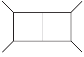
(a) (a)

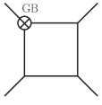
(b) (b)

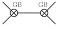
(c) (c)

(d) (d)

Figure 1: Representative four-point diagrams for (a) the bare contribution, and the (b) single-GB-counterterm, (c) double-GB-counterterm, and (d) $R^{3}$-counterterm insertions needed to remove all divergences.

In Ref. PreviousPaper , the same $R^{3}$ divergence (4) was extracted from a four-graviton scattering amplitude with all helicities positive, $M_{4}^{\rm 2-loop}({+}{+}{+}{+})$. This helicity amplitude is particularly simple to calculate, making it a useful probe of the two-loop ultraviolet structure. It is sensitive to the $R^{3}$ operator because the insertion of $R^{3}$ into the tree amplitude gives a nonvanishing result. For a single insertion of the Lagrangian term

$${\cal L}_{R^{3}}\ =\ c_{R^{3}}(\mu)\sqrt{-g}\,R^{\alpha\beta}{\!}_{\gamma\delta}R^{\gamma\delta}{\!}_{\rho\sigma}R^{\rho\sigma}{\!}_{\alpha\beta}\,,$$ (5)

the identical-helicity matrix element is vanNWu

$$M_{4}({+}{+}{+}{+})\ =\ -60\,i\,c_{R^{3}}(\mu)\,\left(\frac{\kappa}{2}\right)^{4}\,{\cal T}^{2}\,s_{12}s_{23}s_{13}\,,$$ (6)

where

$${\cal T}=\frac{[12][34]}{\langle 12\rangle\langle 34\rangle}\,,$$ (7)

and $s_{12}=(k_{1}+k_{2})^{2}$, $s_{23}=(k_{2}+k_{3})^{2}$ and $s_{13}=(k_{1}+k_{3})^{2}$ are the usual Mandelstam invariants. The factor ${\cal T}$ is a pure phase constructed from the spinor products $\langle ab\rangle$ and $[ab]$, defined in e.g. Ref. Review .

Although no mass regulator was used in Ref. PreviousPaper , the Gauss–Bonnet operator (2) contributes nonvanishing subdivergences, because internal legs of the two-loop amplitude propagate in $D$ dimensions. Fig. 1 illustrates the complete set of counterterm contributions required to renormalize the dimensionally-regulated four-graviton amplitude at two loops. Besides the bare amplitude in Fig. 1(a), there is the single insertion of the GB operator into a one-loop amplitude in Fig. 1(b) and the double-GB-counterterm insertion into a tree amplitude, Fig. 1(c). Finally, the two-loop $R^{3}$ counterterm insertion is shown in Fig. 1(d). All contributions shown are representative ones, out of a much larger number of Feynman diagrams; for example, the bare contribution also includes nonplanar diagrams.

For pure gravity, assembling the contributions from Fig. 1(a)–(c), the divergence in the two-loop four-graviton amplitude and associated renormalization-scale dependence is PreviousPaper

$${\cal M}^{{\rm 2\hbox{-}loop}}_{4}({+}{+}{+}{+})\Big{|}_{\rm(a)\hbox{--}(c)}\ =\ \Bigl{(}\frac{\kappa}{2}\Bigr{)}^{6}\frac{i}{(4\pi)^{4}}s_{12}s_{23}s_{13}{\cal T}^{2}\,\biggl{(}\frac{209}{24\,\epsilon}-\frac{1}{4}\,\ln\mu^{2}\biggr{)}+\hbox{finite}\,.$$ (8)

In a minimal subtraction prescription, the effect of the $R^{3}$ counterterm in Fig. 1(d) is simply to remove the $209/24\times 1/\epsilon$ term. Including matter fields, the ultraviolet divergence changes under duality transformations PreviousPaper . This change might not be surprising, given that the coefficient of the one-loop Gauss–Bonnet subdivergence (2) is not invariant under duality transformations DuffInequivalence . For example, adding $n_{3}$ three forms, which do not propagate in four dimensions, changes the coefficient of the infinity in Eq. (4) to

$$\frac{209}{1440\epsilon}\ \rightarrow\ \frac{209}{1440\epsilon}-\frac{1}{8\epsilon}\,n_{3}\,,$$ (9)

while the coefficient of $\ln\mu^{2}$ is unaltered. Also, the value of the leading infinity depends nontrivially on the details of the regularization procedure, while the coefficient of the $\ln\mu^{2}$ term does not.

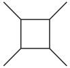
(a) (a)

(b) (b)

Figure 2: Renormalization of on-shell Yang–Mills amplitudes at one loop requires (a) the bare amplitude and (b) an $F^{2}$ counterterm, for which representative contributions are shown.

The fact that the two numerical coefficients in Eq. (8) are rather different, and that one changes under duality transformations but not the other, implies that they are not directly linked. This is rather curious. From the textbook computation of the one-loop beta function in Yang–Mills theory, we are used to the idea that they are linked. In that case, the analog of Fig. 1 is Fig. 2. To renormalize the on-shell amplitudes in the theory at one loop, we need the bare one-loop amplitude, with a representative diagram shown in Fig. 2(a), and a single insertion of the $F^{a}_{\mu\nu}F^{a\,\mu\nu}$ counterterm into a tree-level amplitude, with a representative diagram shown in Fig. 2(b).

Schematically, these two contributions depend on the renormalization scale $\mu$ as follows:

$$\frac{C^{\rm(a)}}{\epsilon}\,(\mu^{2})^{\epsilon}+\frac{C^{\rm(b)}}{\epsilon}\ =\ \Big{(}C^{\rm(a)}+C^{\rm(b)}\Bigr{)}\frac{1}{\epsilon}+C^{\rm(a)}\ln\mu^{2}+\cdots,$$ (10)

where the $(\mu^{2})^{\epsilon}$ factor in the bare amplitude compensates for the dimension of the loop integration measure $d^{4-2\epsilon}\ell$, where $\ell$ is the loop momentum. In a minimal subtraction scheme, one chooses $C^{\rm(b)}=-C^{\rm(a)}$ to cancel the $1/\epsilon$ pole. Because the counterterm insertion has no factor of $(\mu^{2})^{\epsilon}$, the leading divergence $C^{\rm(a)}$ is tied directly to the renormalization-scale dependence of the coupling, i.e. the beta function, independent of the details of the regularization procedure.

What about gravity at two loops? As explained in Ref. PreviousPaper , the disconnect between the divergences and the renormalization-scale dependence happens because of an interplay between the bare terms and the evanescent subdivergences. The analog of Eq. (10) for the divergence and $\ln\mu^{2}$ dependence of the two-loop gravity amplitude is

$$\frac{C^{\rm(a)}}{\epsilon}\,(\mu^{2})^{2\epsilon}+\frac{C^{\rm(b)}}{\epsilon}\,(\mu^{2})^{\epsilon}+\frac{C^{\rm(c)}}{\epsilon}+\frac{C^{\rm(d)}}{\epsilon}=\Big{(}C^{\rm(a)}+C^{\rm(b)}+C^{\rm(c)}+C^{\rm(d)}\Bigr{)}\frac{1}{\epsilon}+(2C^{\rm(a)}+C^{\rm(b)})\ln\mu^{2}+\cdots.$$ (11)

The differing powers of $\mu$ for each contribution follow from dimensional analysis of the integrals, after accounting for the fact that the counterterm insertions do not carry factors of $(\mu^{2})^{\epsilon}$.

The coefficient of the $R^{3}$ counterterm $C^{\rm(d)}$ cancels the two-loop divergence in Eq. (11), as a consequence of the renormalization conditions, $C^{\rm(d)}=-C^{\rm(a)}-C^{\rm(b)}-C^{\rm(c)}$. In the amplitude computed in Ref. PreviousPaper , the value of the coefficient of the two-loop $R^{3}$ counterterm depends on duality transformations, while the coefficient in front of the $\ln\mu^{2}$, namely $2C^{\rm(a)}+C^{\rm(b)}$, does not. The fact that different combinations of coefficients appear in the divergence and in the $\ln\mu^{2}$ term explains why the two-loop divergence and renormalization-scale dependence do not have to be simply related. As we discuss in the next section, the coefficient of the logarithm can be computed directly in four dimensions, completely avoiding the issue of evanescent operators. On the other hand, the divergence is exposed to the subtleties of evanescent operators and dimensional regularization. More remarkably, as found in a variety of examples PreviousPaper , the $\ln\mu^{2}$ coefficient satisfies a simple formula, which we explain in the next section.

The disconnect between the divergence and the renormalization-scale dependence could lead to situations where an explicit divergence is present, yet there is no associated running of a coupling or other physical consequences. As an example, we have computed the divergence in ${\cal N}=1$ supergravity with one matter multiplet using the same techniques. It is convenient to include a matter multiplet because for this theory we can construct the two-loop integrand straightforwardly using double-copy techniques BCJ . Even though this theory is supersymmetric, the trace anomaly is nonvanishing DuffWeyl . Therefore there are subdivergences of the form of Fig. 1(b), as well as Fig. 1(c). We have computed the four contributions corresponding to Fig. 1. They are given by

$$C^{\rm(a)}=\frac{11}{16}\,,\hskip 28.45274ptC^{\rm(b)}=-\frac{11}{8}\,,\hskip 28.45274ptC^{\rm(c)}=\frac{363}{32}\,,\hskip 28.45274ptC^{\rm(d)}=-\frac{341}{32}\,,$$ (12)

where the normalization corresponds to $C^{\rm(a)}+C^{\rm(b)}+C^{\rm(c)}=209/24$ for pure gravity; see Eq. (8). So the divergence from terms (a)–(c) in Eq. (11) is nonzero, but the $\ln\mu^{2}$ coefficient vanishes, $2C^{\rm(a)}+C^{\rm(b)}=0$. In fact, it turns out that all logarithms $\ln s_{ij}$ in the amplitude cancel as well. The polynomial terms can be canceled by the same $R^{3}$ counterterm but with a finite coefficient (or equivalently, an order $\epsilon$ correction to $C^{\rm(d)}$).

The upshot is that for this ${\cal N}=1$ supergravity theory, the divergence and associated trace anomaly has the curious effect of violating the supersymmetry Ward identity SWI that requires the identical-helicity amplitude to vanish. The appearance of a divergence is due to the breaking of supersymmetry by the trace anomaly, which induces subdivergences even when supersymmetry implies that no divergences can be present TwoLoopSusy . To restore the supersymmetry Ward identities requires adding an $R^{3}$ counterterm to the theory, with both a $1/\epsilon$ and a finite coefficient, which fixes the two-loop amplitude uniquely. This procedure is possible only because the $\ln\mu^{2}$ coefficient vanishes. That is, in this case there is no loss of predictivity, even though there is a $1/\epsilon$ divergence. If the $\ln\mu^{2}$ coefficient is nonvanishing, as in the case of pure gravity, then there must be an arbitrary finite constant in the renormalization procedure, associated with fixing the $R^{3}$ coupling at different choices of renormalization scale, leading to the usual loss of predictivity of nonrenormalizable theories.

This discussion applies more generally. Suppose there is a hidden symmetry that would enforces finiteness if it can be preserved. Yet if that symmetry is broken by the trace anomaly, or more generally by the regularization procedure, we might conclude that the theory’s divergence implies a loss of predictivity. It is therefore always crucial to inspect the renormalization-scale dependence.

In contrast, one might even imagine a regularization prescription that eliminates the $1/\epsilon$ divergence, for example by making the perverse choice $n_{3}=8\cdot 209/1440$ in Eq. (9) for the case of pure gravity. However, since the $\ln\mu^{2}$ coefficient is nonvanishing in this case, there is still an arbitrariness in the finite $R^{3}$ counterterm associated with different choices for $\mu$, and an associated loss of predictivity. The theory is no better than an ultraviolet-divergent theory, even if the $1/\epsilon$ divergence is arranged to cancel.

From now on we focus entirely on the renormalization-scale dependence. For the two-loop graviton identical-helicity scattering amplitude with various matter content, Ref. PreviousPaper found the following simple form:

$${\cal M}^{{\rm 2\hbox{-}loop}}_{4}({+}{+}{+}{+})\Bigr{|}_{\ln\mu^{2}}\ =\ -\Bigl{(}\frac{\kappa}{2}\Bigr{)}^{6}\frac{i}{(4\pi)^{4}}s_{12}s_{23}s_{13}{\cal T}^{2}\,\frac{N_{b}-N_{\!f}}{8}\,\ln\mu^{2}\,,$$ (13)

where $N_{b}$ and $N_{\!f}$ are the number of physical four-dimensional bosonic and fermionic states in the theory. Using Eq. (6), this result is equivalent to the running of the $R^{3}$ coefficient according to

$$\mu\frac{\partial\,c_{R^{3}}}{\partial\mu}\ =\ \Bigl{(}\frac{\kappa}{2}\Bigr{)}^{2}\frac{1}{(4\pi)^{4}}\,\frac{N_{b}-N_{\!f}}{240}\,.$$ (14)

Because the number of physical four-dimensional states does not change under duality transformations, this equation is automatically independent of such transformations and of the details of the regularization scheme. In fact, the result was only confirmed in Ref. PreviousPaper for minimally-coupled scalars, antisymmetric tensors and (non-propagating) three-form fields. The generalization to fermionic contributions was based on the previously-mentioned supersymmetry Ward identities. It is quite remarkable that such a simple formula for the renormalization-scale dependence emerges from the computations carried out in Ref. PreviousPaper . How did this happen? We answer this in the next section.

III Renormalization-scale dependence directly from four-dimensional unitarity cuts

In this section we explain the simple form of the renormalization-scale dependence in Eq. (13) using four-dimensional unitarity cuts. We show that it holds for any massless theory with minimal couplings to gravity and renormalizable matter interactions. From simple dimensional considerations, contributions to the $R^{3}$ operator necessarily involve couplings with the dimension of the gravitational coupling $\kappa$, which carries the dimension of inverse mass, $1/M_{P}$. Renormalizable matter interactions are either dimensionless or carry the dimension of mass, so they can contribute only to lower-dimension operators than $R^{3}$ at two loops, and therefore they are not relevant at this order. We will also explain why dilatons and antisymmetric tensors—whose minimal couplings to gravitons have two derivatives, as does pure gravity—also respect Eq. (13), as found in the computations of Refs. PreviousPaper ; DoubleCopyGravity .

Unitarity cuts are not directly sensitive to the $\ln\mu^{2}$ dependence. However, in a massless theory, simple dimensional analysis relates the coefficient of $\ln\mu^{2}$ to the coefficients of logarithms of kinematic invariants, $\ln s_{ij}$, because the arguments of all logarithms need to be dimensionless. Because the coefficient of $\ln\mu^{2}$ is finite, we can evaluate the unitarity cuts in four dimensions (after subtracting a universal infrared divergence). Thus we automatically avoid evanescent operators, such as the Gauss–Bonnet term (2). Our approach greatly clarifies the essential physics, showing that duality transformations cannot change the logarithms in the scattering amplitude, because in four dimensions, unlike $D$ dimensions, duality does not change the Lorentz properties or number of physical states. The calculation of the logarithms using unitarity cuts was carried out long ago by Dunbar and Norridge DunbarNorridge . Recently a similar technique has been applied to two-loop identical-helicity amplitudes in gauge theory by Dunbar, Jehu and Perkins DunbarJehuPerkins . Here we repeat the two-loop four-graviton calculation, but in a way that completely avoids dimensional regularization and focuses on the consequences and interpretation of the renormalization scale.

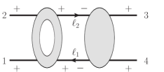
(a) (a)

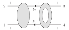
(b) (b)

Figure 3: The $s$-channel two-particle cuts (a) and (b) from which we can extract the logarithmic parts of the two-loop four-point identical-helicity four-graviton amplitude. The exposed lines are placed on shell and are in four dimensions.

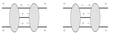
Figure 4: Representative contributions to the three-particle cut. This cut generates no new $\ln\mu^{2}$ contributions to the $R^{3}$ operator for the identical-helicity four-graviton amplitude.

We obtain the kinematical logarithms of the all-plus helicity amplitude from the four-dimensional unitarity cuts. At two loops, there are cuts where two particles cross the cut, illustrated in Fig. 3, and where three particles cross the cut, shown in Fig. 4. In four dimensions, many contributions to these cuts vanish, because the tree amplitude on one side of a cut vanishes.

In pure gravity, all contributions to the three-particle cuts shown in Fig. 4 vanish, because they contain a either a tree amplitude with all identical helicities, or one with one leg of opposite helicity. Such five-graviton tree amplitudes vanish. Adding minimally-coupled matter does not alter this conclusion. As already noted, adding matter with renormalizable self couplings cannot affect the coefficient of the $R^{3}$ operator. Similarly, dilatons and antisymmetric tensors, with their minimal couplings to each other and to gravity also cannot contribute, because their amplitudes have similar vanishings as the pure gravity case, where a pair of external (pseudo)scalar state should be assigned one plus and one minus helicity. All of these vanishings can be understood from the fact that all such amplitudes can be constructed from minimally-coupled gauge theory via the Kawai–Lewellen–Tye (KLT) relations KLT , which all have the corresponding vanishings. Alternatively, such tree amplitudes can be embedded into ${\cal N}=8$ supergravity, and then the supersymmetry Ward identities SWI imply the required vanishings.

The two-particle cut does have nonvanishing contributions; however, the cut lines have to be gravitons, with the helicity configurations displayed in Fig. 3. If a massless particle other than a graviton crosses the cut with this helicity configuration, then the tree amplitude entering the cut necessarily vanishes. These vanishings can be understood in various ways. The KLT decomposition offers one such way. Consider the KLT decomposition of the gravitational tree amplitude on the right-hand side of Fig. 3(a) into a product of two gauge-theory amplitudes KLT ,

$$M^{\rm tree}(\ell_{1},-\ell_{2},3,4)=s_{12}\,A^{\rm tree}(\ell_{1},-\ell_{2},3,4)A^{\rm tree}(\ell_{1},-\ell_{2},4,3)\,,$$ (15)

where $M^{\rm tree}(1,2,3,4)$ is the gravitational tree amplitude and $A^{\rm tree}(1,2,3,4)$ is a color-ordered Yang–Mills tree amplitude. (In this expression the couplings are stripped off.) If legs $3$ and $4$ of the gravitational amplitude are positive-helicity gravitons in an all-outgoing convention, then the corresponding legs in the gauge-theory amplitudes are positive-helicity gluons, so that the spins match. For gauge-theory amplitudes where legs $3$ and $4$ are positive-helicity gluons, the only nonvanishing configuration is where the remaining two legs are negative-helicity gluons. The KLT relations then imply that the only nonvanishing gravity tree amplitude is when the two legs labeled by $\ell_{1}$ and $-\ell_{2}$ in the unitarity cut are gravitons with negative helicity. Other configurations, corresponding to particles other than negative-helicity gravitons, vanish because at least one of the corresponding gauge-theory amplitudes vanishes.

A consequence of these restrictions is that the one-loop amplitude appearing on the other side of the two-particle cut must be an all-plus-helicity amplitude with only external gravitons. Such amplitudes are remarkably simple DunbarNorridge . This simplicity enormously streamlines the calculation of the cut. There are two contributions to the $s_{12}$-channel cut, shown in Fig. 3(a) and (b), depending on whether the loop amplitude is located on the left or right side of the cut. However, they give equal contributions, because Fig. 3(b) can be mapped back to Fig. 3(a) by relabeling the momenta by $k_{i}\to k_{i+2}$, where the indices are modulo 4, and we will see that the cut is invariant under this operation. In addition to the $s_{12}$-channel cut displayed in Fig. 3, there are also cuts in the $s_{23}$ and $s_{13}$ channels, which can be obtained from the $s_{12}$ channel by Bose symmetry, permuting $k_{1}\leftrightarrow k_{3}$ and $k_{1}\leftrightarrow k_{4}$, respectively.

The required one-loop amplitude with four identical-helicity gravitons is DunbarNorridge ,

$$M^{{\rm 1\hbox{-}loop}}(1^{+},2^{+},3^{+},4^{+})\ =\ -\frac{i}{(4\pi)^{2}}\frac{N_{b}-N_{\!f}}{240}\biggl{(}\frac{\kappa}{2}\biggr{)}^{4}\,{\cal T}^{2}\,(s_{12}^{2}+s_{14}^{2}+s_{24}^{2})\,,$$ (16)

where the permutation-invariant, pure-phase spinor combination ${\cal T}$ is defined in Eq. (7). The one-loop external graviton amplitude is unaffected by any interactions of the matter fields in a minimally-coupled theory: at one loop with all external gravitons there are no diagrams containing matter self-interactions.

In Yang–Mills theory, Bardeen and Cangemi AllPlusAnomaly argued that the corresponding identical-helicity amplitude is nonvanishing because of an anomaly in the infinite-dimensional symmetry of the self-dual sector of the theory. Presumably, the same holds in gravity. It is quite interesting that this anomaly-like behavior appears crucial for obtaining a nonvanishing one-loop four-graviton amplitude, which as we will see below leads to a nonvanishing coefficient of the $\ln\mu^{2}$ term.

We also need the four-graviton tree amplitude. It is easily obtained from the KLT relation KLT ,

$$M^{{\rm tree}}(1^{-},2^{-},3^{+},4^{+}) = -i\biggl{(}\frac{\kappa}{2}\biggr{)}^{2}s_{12}\,A^{\rm tree}(1,2,3,4)A^{\rm tree}(1,2,4,3)$$ (17)

$$= i\biggl{(}\frac{\kappa}{2}\biggr{)}^{2}s_{12}\,\frac{{\left\langle 1\,2\right\rangle}^{3}}{\left\langle 2\,3\right\rangle\left\langle 3\,4\right\rangle\left\langle 4\,1\right\rangle}\,\frac{{\left\langle 1\,2\right\rangle}^{3}}{\left\langle 2\,4\right\rangle\left\langle 4\,3\right\rangle\left\langle 3\,1\right\rangle}\,.$$

We now calculate the unitarity cut in Fig. 3(a). The cut integrand is given by the relabeled product of Eqs. (16) and (17),

$$C_{12} = {\cal N}\,s_{12}\,(s_{12}^{2}+s_{1\ell_{1}}^{2}+s_{2\ell_{1}}^{2})$$ (18)

$$\times\biggl{(}\frac{\left[1\,2\right]\left[\ell_{2}\,(-\ell_{1})\right]}{\left\langle 1\,2\right\rangle\left\langle\ell_{2}\,(-\ell_{1})\right\rangle}\biggr{)}^{2}\frac{\left\langle\ell_{1}\,(-\ell_{2})\right\rangle^{3}}{\left\langle(-\ell_{2})\,3\right\rangle\left\langle 3\,4\right\rangle\left\langle 4\,\ell_{1}\right\rangle}\,\frac{\left\langle\ell_{1}\,(-\ell_{2})\right\rangle^{3}}{\left\langle(-\ell_{2})\,4\right\rangle\left\langle 4\,3\right\rangle\left\langle 3\,\ell_{1}\right\rangle}\,,$$

where the labels follow Fig. 3(a) and the normalization factor is

$${\cal N}=\frac{1}{(4\pi)^{2}}\frac{N_{b}-N_{\!f}}{240}\biggl{(}\frac{\kappa}{2}\biggr{)}^{6}\,.$$ (19)

Rearranging the spinor products and using the identity $1/\left\langle a\,b\right\rangle=[ba]/(k_{a}+k_{b})^{2}$ gives

$$C_{12} = {\cal N}\,{\cal T}^{2}\,s_{12}\,(s_{12}^{2}+s_{1\ell_{1}}^{2}+s_{2\ell_{1}}^{2})$$ (20)

$$\times\frac{\left\langle\ell_{1}\,\ell_{2}\right\rangle\left[\ell_{2}\,3\right]\left\langle 3\,4\right\rangle\left[4\,\ell_{1}\right]\left\langle\ell_{1}\,\ell_{2}\right\rangle\left[\ell_{2}\,4\right]\left\langle 4\,3\right\rangle\left[3\,\ell_{1}\right]}{(\ell_{2}-k_{3})^{2}(\ell_{1}+k_{4})^{2}(\ell_{2}-k_{4})^{2}(\ell_{1}+k_{3})^{2}}\,.$$

The net effect of replacing $-\ell_{1}$ and $-\ell_{2}$ with $\ell_{1}$ and $\ell_{2}$ is a factor of $+1$. We can simplify $C_{12}$ further by observing that the numerator forms a trace,

$$\left\langle\ell_{1}\,\ell_{2}\right\rangle\left[\ell_{2}\,3\right]\left\langle 3\,4\right\rangle\left[4\,\ell_{1}\right]\left\langle\ell_{1}\,\ell_{2}\right\rangle\left[\ell_{2}\,4\right]\left\langle 4\,3\right\rangle\left[3\,\ell_{1}\right] = \frac{1}{2}\,{\rm tr}[(1-\gamma_{5})\ell_{1}\ell_{2}k_{3}k_{4}\ell_{1}\ell_{2}k_{4}k_{3}]$$ (21)

$$= (\ell_{1}+k_{3})^{2}(\ell_{1}+k_{4})^{2}s_{34}^{2}\,,$$

where we used $\ell_{2}=\ell_{1}+k_{3}+k_{4}$ and the on-shell conditions $\ell_{1}^{2}=\ell_{2}^{2}=0$ to simplify the trace. Thus, the numerator cancels the (doubled) propagators leaving

$$C_{12} = {\cal N}{\cal T}^{2}\,s_{12}^{3}\,\frac{s_{12}^{2}+s_{1\ell_{1}}^{2}+s_{2\ell_{1}}^{2}}{(\ell_{2}-k_{3})^{2}(\ell_{2}-k_{4})^{2}}$$ (22)

$$= -{\cal N}{\cal T}^{2}\,s_{12}^{2}\,(s_{12}^{2}+s_{1\ell_{1}}^{2}+s_{2\ell_{1}}^{2})\biggl{[}\frac{1}{(\ell_{1}+k_{4})^{2}}+\frac{1}{(\ell_{1}+k_{3})^{2}}\biggr{]}\,.$$

This expression for the cut actually has an infrared divergence when integrated over phase space. However, this divergence is harmless because infrared singularities of gravity theories are relatively simple IRPapers . The source of the singularity is from exchange of soft virtual gravitons with momentum $\ell_{1}+k_{3}$ or $\ell_{1}+k_{4}$; the soft limit is when $\ell_{1}\rightarrow-k_{4}$ or $\ell_{1}\rightarrow-k_{3}$, for the first or second term in Eq. (22), respectively. To remove the infrared singularity, we simply subtract the soft limit of the integrand, replacing $C_{12}$ by

$$\tilde{C}_{12}=-{\cal N}{\cal T}^{2}\,s_{12}^{2}\,\frac{s_{1\ell_{1}}^{2}+s_{2\ell_{1}}^{2}-s_{14}^{2}-s_{24}^{2}}{(\ell_{1}+k_{4})^{2}}+(k_{3}\leftrightarrow k_{4}).$$ (23)

The subtraction terms correspond to cut scalar triangle integrals. Since the triangle integrals that are subtracted converge in the ultraviolet, the subtraction has no effect on the ultraviolet logarithms with which we are concerned here.

The discontinuity is obtained by integrating over the Lorentz-invariant phase space,

$$I_{12}\ =\ \int{\rm dLIPS}\,\tilde{C}_{12}\ =\ -{\cal N}{\cal T}^{2}\,s_{12}^{3}\hat{I}_{12}+(k_{3}\leftrightarrow k_{4})\,,$$ (24)

where

$$\hat{I}_{12}\ =\ \int{\rm dLIPS}\,\frac{(2k_{1}\cdot\ell_{1})^{2}+(2k_{2}\cdot\ell_{1})^{2}-s_{14}^{2}-s_{24}^{2}}{s_{12}\,(2k_{4}\cdot\ell_{1})}\,.$$ (25)

We perform the phase-space integration in the center-of-mass frame, parametrizing the external momenta as

$$k_{1} = \frac{\sqrt{s}}{2}(-1,\,\sin\theta\cos\phi,\,\sin\theta\sin\phi,\,\cos\theta)\,,$$

$$k_{2} = \frac{\sqrt{s}}{2}(-1,\,-\sin\theta\cos\phi,\,-\sin\theta\sin\phi,\,-\cos\theta)\,,$$

$$k_{3} = \frac{\sqrt{s}}{2}(1,\,0,\,0,\,1)\,,$$

$$k_{4} = \frac{\sqrt{s}}{2}(1,\,0,\,0,\,-1)\,,$$ (26)

and the internal momentum as

$$\ell_{1} = \frac{\sqrt{s}}{2}(-1,\,\sin\hat{\theta}\cos\hat{\phi},\,\sin\hat{\theta}\sin\hat{\phi},\,\cos\hat{\theta})\,,$$ (27)

while $-\ell_{2}^{0}=\ell_{1}^{0}$ and $-\vec{\ell}_{2}=-\vec{\ell}_{1}$. The on-shell conditions enforce the constraints $|\ell_{i}^{0}|=|\vec{\ell}_{i}|=\sqrt{s}/2$, $i=1,2$. The standard two-body phase-space measure is

$$\int{\rm dLIPS}\ =\ \frac{1}{2}\frac{1}{8\pi}\int_{-1}^{1}\frac{d\cos\hat{\theta}}{2}\int_{0}^{2\pi}\frac{d\phi}{2\pi}\,.$$ (28)

There is an extra Bose symmetry factor of $1/2$ because two identical-helicity gravitons cross the cut. Substituting the momentum parametrization into Eq. (25) gives an expression for $\hat{I}_{12}$ purely in terms of angular variables, which can be integrated easily,

$$\hat{I}_{12} = \frac{1}{16\pi}\int_{-1}^{1}\frac{d\cos\hat{\theta}}{2}\int_{0}^{2\pi}\frac{d\hat{\phi}}{2\pi}\frac{1}{1-\cos\hat{\theta}}\Bigl{[}\cos^{2}\theta\,\sin^{2}\hat{\theta}-\sin^{2}\theta\,\sin^{2}\hat{\theta}\,\cos^{2}(\phi-\hat{\phi})$$ (29)

$$\hskip 156.49014pt\hbox{}-\frac{1}{2}\sin 2\theta\,\sin 2\hat{\theta}\,\cos(\phi-\hat{\phi})\Bigr{]}$$

$$= \frac{1}{16\pi}\int_{-1}^{1}\frac{d\cos\hat{\theta}}{2}\frac{1}{1-\cos\hat{\theta}}\Bigl{[}\cos^{2}\theta\,\sin^{2}\hat{\theta}-\frac{1}{2}\sin^{2}\theta\,\sin^{2}\hat{\theta}\Bigr{]}$$

$$= \frac{1}{16\pi}\Bigl{[}\cos^{2}\theta-\frac{1}{2}\sin^{2}\theta\Bigr{]}\int_{-1}^{1}\frac{d\cos\hat{\theta}}{2}[1+\cos\hat{\theta}]$$

$$= \frac{2-3\sin^{2}\theta}{32\pi}\,.$$

Using $s_{13}s_{23}=(s_{12}^{2}/4)\times\sin^{2}\theta$, we can re-express the answer in a Lorentz-invariant form:

$$\hat{I}_{12}\ =\ \frac{1}{16\pi}\frac{s_{12}^{2}-6s_{13}\,s_{23}}{s_{12}^{2}}\,.$$ (30)

Since this result is invariant under $k_{3}\rightarrow k_{4}$, the exchange contribution in Eq. (24) just gives a factor of 2.

Putting it all together, we have

$$\tilde{C}_{12} = -\frac{{\cal N}{\cal T}^{2}}{8\pi}\ s_{12}\,(s_{12}^{2}-6s_{13}\,s_{23})$$ (31)

$$= 2\pi i\left[\frac{i}{(4\pi)^{4}}\frac{N_{b}-N_{\!f}}{240}\left(\frac{\kappa}{2}\right)^{6}{\cal T}^{2}s_{12}(s_{12}^{2}-6s_{13}\,s_{23})\right].$$ (32)

We extracted a factor of $2\pi i$ because the analytic continuation of $\ln(-s_{ij}/\mu^{2})$ from below the cut ($s_{ij}\to s_{ij}-i\varepsilon$) to above the cut ($s_{ij}\to s_{ij}+i\varepsilon$) is

$$\ln\biggl{(}\frac{-s_{ij}}{\mu^{2}}\biggr{)}\ \to\ \ln\biggl{(}\frac{-s_{ij}}{\mu^{2}}\biggr{)}-2\pi i\,.$$ (33)

Thus, the $s_{12}$-channel discontinuity we computed is related to the coefficient of $\ln\mu^{2}$ by

$$M^{\rm 2-loop}|_{\ln\mu^{2}}\ =\ \frac{1}{2\pi i}M^{\rm 2-loop}|_{\rm disc}\times\ln\mu^{2}\,.$$ (34)

We also need to multiply by a factor of 2 for the contribution of Fig. 3(b), and include the contributions of the other two channels, using

$$s_{12}(s_{12}^{2}-6s_{13}\,s_{23})\ +\ (k_{1}\leftrightarrow k_{3})\ +\ (k_{1}\leftrightarrow k_{4})=s_{12}^{3}+s_{23}^{3}+s_{13}^{3}-18s_{12}s_{23}s_{13}=-15s_{12}s_{23}s_{13}\,.$$ (35)

We obtain

$$M^{\rm 2-loop}({+}{+}{+}{+})\Bigl{|}_{\ln\mu^{2}}\ =\ -\left(\frac{\kappa}{2}\right)^{6}\frac{i}{(4\pi)^{4}}s_{12}s_{23}s_{13}{\cal T}^{2}\,\frac{N_{b}-N_{f}}{8}\ln\mu^{2}.$$ (36)

Thus, we have derived the simple renormalization-scale dependence of the two-loop four-graviton amplitude PreviousPaper , but now in a way that avoids reliance on evanescent operators or other subtleties of dimensional regularization. Given that only four-dimensional quantities were used, duality transformations manifestly cannot affect the renormalization-scale dependence.

IV Conclusions

In this paper we explained the simple form of the renormalization-scale dependence of two-loop gravity amplitudes proposed in Ref. PreviousPaper . While the two-loop ultraviolet divergence in dimensional regularization changes under duality transformations, and is afflicted by evanescent subdivergences, the renormalization-scale dependence is remarkably simple PreviousPaper . In order to explain its simple form, we used four-dimensional unitarity cuts, which effectively converted the two-loop computation into a one-loop one. As in Ref. PreviousPaper , we studied the identical-helicity amplitude, because it is particularly simple to evaluate, yet is sensitive to the two-loop $R^{3}$ ultraviolet divergence. While the renormalization scale $\ln\mu^{2}$ does not itself have a unitarity cut, on dimensional grounds its coefficient must balance the coefficients of the logarithms of kinematic variables, thus allowing us to extract the $\ln\mu^{2}$ coefficient directly from the unitarity cuts. This method avoids the need for ultraviolet regularization, as well as all subtleties associated with evanescent operators. A trivial integral over the two-body phase space for intermediate gravitons is all that is required to explain the simple formula (36) of Ref. PreviousPaper .

A rather interesting property of the gravity divergence is that it appears to be tied to an anomaly. In Yang–Mills theory, the nonvanishing of the one-loop identical helicity amplitude has been tied to an anomaly in the conserved currents of self-dual Yang–Mills theory AllPlusAnomaly . We expect gravity to be similar. Integrability has been used to construct classical self-dual solutions to Einstein’s equations SDGIntegrable . It is natural to conjecture that a quantum anomaly in the conservation of the associated currents of self-dual gravity Krasnov could be responsible for the non-vanishing one-loop amplitude (16) which underlies the two-loop $\ln\mu^{2}$ dependence. In any case, not only the two-loop divergence but the nonvanishing of the one- and two-loop identical-helicity amplitudes can be traced to an $\epsilon/\epsilon$ effect in dimensional regularization, similar to the way that chiral and other anomalies arise. It would be quite enlightening if we could link the pure gravity divergence, or more importantly, the nonvanishing renormalization-scale dependence, more directly to an anomaly.

In this paper we considered the identical-helicity amplitude, because it is the simplest helicity configuration that is sensitive to the $R^{3}$ divergence. It would be interesting to evaluate the other helicity configurations to corroborate our understanding. The other helicity configurations are significantly more complicated, because the three-particle cut no longer vanishes in four dimensions. However, the $({-}{+}{+}{+})$ helicity configuration, which also receives contributions from the $R^{3}$ operator, should be tractable using four-dimensional unitarity cuts.

Usually in field theory, the first dimensionally-regulated divergence that is encountered is directly related to the renormalization-scale dependence of either a coupling (i.e. the beta function) or the coefficient of an operator (i.e. its anomalous dimension). Pure Einstein gravity at two loops provides an explicit counterexample to this expectation, but it is probably not the only one. As we discussed in Section II, the key feature is that a candidate operator for a first divergence is evanescent, vanishing in four dimensions but not in $D$ dimensions. The different $\mu$ dependence associated with the bare and counterterm contributions spoils the textbook relation between the pole in $\epsilon$ and the renormalization-scale dependence at the following loop order. Another place this might happen is in the effective field theory of long flux tubes OferZohar . The key lessons are that ultraviolet divergences in dimensional regularization have to be treated with caution in certain circumstances, and that it is safer to focus on the more physical renormalization-scale dependence of the renormalized theory.

Acknowledgments

We thank Clifford Chueng, Scott Davies, David Kosower and Josh Nohle for many useful and interesting discussions. We also thank Michael Duff for pointing out the curious issue posed by a non-vanishing trace anomaly in ${\cal N}=1$ supergravity. This material is based upon work supported by the Department of Energy under Award Number DE-SC0009937 and contract DE-AC02-76SF00515.

References

- (1) Z. Bern, S. Davies, T. Dennen and Y.-t. Huang, Phys. Rev. Lett. 108, 201301 (2012) [arXiv:1202.3423 [hep-th]]; Phys. Rev. D 86, 105014 (2012) [arXiv:1209.2472 [hep-th]].
- (2) Z. Bern, S. Davies and T. Dennen, Phys. Rev. D 90, 105011 (2014) [arXiv:1409.3089 [hep-th]].
-
(3)
G. Bossard, P. S. Howe and K. S. Stelle,
Phys. Lett. B 719, 424 (2013)
[arXiv:1212.0841 [hep-th]];
G. Bossard, P. S. Howe and K. S. Stelle, JHEP 1307, 117 (2013) [arXiv:1304.7753 [hep-th]];
Z. Bern, S. Davies and T. Dennen, Phys. Rev. D 88, 065007 (2013) [arXiv:1305.4876 [hep-th]]. -
(4)
M. H. Goroff and A. Sagnotti,
Phys. Lett. B 160, 81 (1985);
M. H. Goroff and A. Sagnotti, Nucl. Phys. B 266, 709 (1986). - (5) A. E. M. van de Ven, Nucl. Phys. B 378, 309 (1992).
- (6) Z. Bern, C. Cheung, H. H. Chi, S. Davies, L. Dixon and J. Nohle, Phys. Rev. Lett. 115, 211301 (2015) [arXiv:1507.06118 [hep-th]].
- (7) G. ’t Hooft and M. J. G. Veltman, Annales Poincare Phys. Theor. A 20, 69 (1974).
- (8) M. J. Duff and P. van Nieuwenhuizen, Phys. Lett. B 94, 179 (1980).
-
(9)
E. Sezgin and P. van Nieuwenhuizen,
Phys. Rev. D 22, 301 (1980);
E. S. Fradkin and A. A. Tseytlin, Phys. Lett. B 137, 357 (1984). - (10) W. Siegel, Phys. Lett. B 103, 107 (1981).
-
(11)
E. S. Fradkin and A. A. Tseytlin,
Annals Phys. 162, 31 (1985);
M. T. Grisaru, N. K. Nielsen, W. Siegel and D. Zanon, Nucl. Phys. B 247, 157 (1984). -
(12)
A. J. Buras and P. H. Weisz,
Nucl. Phys. B 333, 66 (1990);
M. J. Dugan and B. Grinstein, Phys. Lett. B 256, 239 (1991);
I. Jack, D. R. T. Jones and K. L. Roberts, Z. Phys. C 63, 151 (1994) [hep-ph/9401349];
S. Herrlich and U. Nierste, Nucl. Phys. B 455, 39 (1995) [hep-ph/9412375];
R. Harlander, P. Kant, L. Mihaila and M. Steinhauser, JHEP 0609, 053 (2006) [hep-ph/0607240]. - (13) O. Aharony and Z. Komargodski, JHEP 1305, 118 (2013) [arXiv:1302.6257 [hep-th]].
-
(14)
D. M. Capper and M. J. Duff,
Nuovo Cim. A 23, 173 (1974);
D. M. Capper and M. J. Duff, Phys. Lett. A 53, 361 (1975);
H. S. Tsao, Phys. Lett. B 68, 79 (1977);
G. W. Gibbons, S. W. Hawking and M. J. Perry, Nucl. Phys. B 138, 141 (1978);
R. Critchley, Phys. Rev. D 18, 1849 (1978). - (15) D. M. Capper and D. Kimber, J. Phys. A 13, 3671 (1980).
- (16) P. van Nieuwenhuizen and C. C. Wu, J. Math. Phys. 18, 182 (1977).
- (17) M. L. Mangano and S. J. Parke, Phys. Rept. 200, 301 (1991) [hep-th/0509223].
- (18) Z. Bern, J. J. M. Carrasco and H. Johansson, Phys. Rev. D 78, 085011 (2008) [arXiv:0805.3993 [hep-ph]]; Phys. Rev. Lett. 105, 061602 (2010) [arXiv:1004.0476 [hep-th]].
- (19) M. J. Duff, Class. Quant. Grav. 11, 1387 (1994) [hep-th/9308075].
-
(20)
M. T. Grisaru, H. N. Pendleton and P. van Nieuwenhuizen,
Phys. Rev. D 15, 996 (1977);
M. T. Grisaru and H. N. Pendleton, Nucl. Phys. B 124, 81 (1977);
S. J. Parke and T. R. Taylor, Phys. Lett. B 157, 81 (1985) Erratum: [Phys. Lett. B 174, 465 (1986)]. -
(21)
E. Tomboulis,
Phys. Lett. B 67, 417 (1977);
M. T. Grisaru, Phys. Lett. B 66, 75 (1977). -
(22)
H. Kawai, D. C. Lewellen and S. H. H. Tye,
Nucl. Phys. B 269, 1 (1986)
F. A. Berends, W. T. Giele and H. Kuijf,
Phys. Lett. B 211, 91 (1988);
Z. Bern, L. J. Dixon, M. Perelstein and J. S. Rozowsky, Nucl. Phys. B 546, 423 (1999) [hep-th/9811140]. - (23) Z. Bern, S. Davies, T. Dennen, Y.-t. Huang and J. Nohle, Phys. Rev. D 92, 045041 (2015) [arXiv:1303.6605 [hep-th]].
- (24) D. C. Dunbar and P. S. Norridge, Nucl. Phys. B 433, 181 (1995) [hep-th/9408014].
-
(25)
D. C. Dunbar and W. B. Perkins,
Phys. Rev. D 93, 085029 (2016)
[arXiv:1603.07514 [hep-th]];
D. C. Dunbar, G. R. Jehu and W. B. Perkins, Phys. Rev. Lett. 117, 061602 (2016) [arXiv:1605.06351 [hep-th]];
Phys. Rev. D 93, 125006 (2016) [arXiv:1604.06631 [hep-th]]. -
(26)
W. A. Bardeen,
Prog. Theor. Phys. Suppl. 123, 1 (1996);
D. Cangemi, Nucl. Phys. B 484, 521 (1997) [hep-th/9605208]; Int. J. Mod. Phys. A 12, 1215 (1997) [hep-th/9610021]. -
(27)
S. Weinberg,
Phys. Rev. 140, B516 (1965);
S. G. Naculich and H. J. Schnitzer,
JHEP 1105, 087 (2011)
[arXiv:1101.1524 [hep-th]];
S. G. Naculich, H. Nastase and H. J. Schnitzer, JHEP 1304, 114 (2013) [arXiv:1301.2234 [hep-th]];
R. Akhoury, R. Saotome and G. Sterman, Phys. Rev. D 84, 104040 (2011) [arXiv:1109.0270 [hep-th]]. -
(28)
R. S. Ward,
Phil. Trans. Roy. Soc. Lond. A 315, 451 (1985);
Q. H. Park, Phys. Lett. B 297, 266 (1992) [hep-th/9211037];
M. Dunajski, L. J. Mason and N. M. J. Woodhouse, J. Phys. A: Math. Gen. 31, 6019 (1998). - (29) K. Krasnov, arXiv:1610.01457 [hep-th].