Ab initio dynamical exchange interactions in frustrated anti-ferromagnets

Abstract

The ultrafast response to an optical pulse excitation of the spin-spin exchange interaction in transition metal anti-ferromagnets is studied within the framework of the time-dependent spin-density functional theory. We propose a formulation for the purely dynamical exchange interaction, which is non-local in space, and it is derived starting from ab initio arguments. Then, we investigate the effect of the laser pulse on the onset of the dynamical process. It is found that we can distinguish two types of excitations, both activated immediately after the action of the laser pulse. While the first one can be associated to a Stoner-like excitation and involves the transfer of spin from one site to another, the second one is related to the ultrafast modification of a Heisenberg-like exchange interaction and can trigger the formation of spin waves in the first few hundred femtoseconds of the time evolution.

I Introduction

Density functional theory (DFT) has been the workhorse in material properties prediction from first principles for nearly half of a century. Among the many physical quantities that can be extracted from DFT, particularly relevant for magnetism is the evaluation of the static Heisenberg exchange parameters Kat00 ; Kat04 ; Loun10 . Their calculation has been closely related to and motivated by the problem of theoretically predicting the finite-temperature properties of magnetic systems. A possible approach consists in assuming that the magnetic excitations can be reasonably described by a Heisenberg-like Hamiltonian of the following form

$$H=-\frac{1}{2N}\sum_{m\neq n}J_{mn}\,\mathbf{S}_{m}\cdot\mathbf{S}_{n}\>,$$ (1)

where $\mathbf{S}_{m}$ designates the spin vector associated to the site $m$, $J_{mn}$ is the exchange interaction between the spins at the two sites $m$ and $n$, and $N$ is the number of unit cells in the macroscopic system. If one considers a low energy excitation of the magnetic system described in terms of a spin spiral solution with wave vector $\mathbf{q}$ and polar angle $\theta$, the difference in total energy between this configuration, $E(\mathbf{q},\theta)$, and the reference ferromagnetic one, $E(\mathbf{0},\theta)$, will be in general related to the magnon frequency $\omega_{\mathbf{q}}$. In case of a single magnetic sublattice it can be shown that EXCH3

$$\omega_{\mathbf{q}}=4\frac{E(\mathbf{q},\theta)-E(\mathbf{0},\theta)}{M\sin^{2}\theta}\>,$$ (2)

where $M$ is the magnitude of the onsite magnetization. Such frequency can be in turn related to the exchange parameter, $J(\mathbf{q})$, through the relation $\omega_{\mathbf{q}}=2[J(\mathbf{0})-J(\mathbf{q})]/M$. By employing the magnetic force theorem MFT ; MFT2 ; EXCH , the difference in total energy between the two magnetic configurations can be related to the difference in the sum of the single particle energies calculated at the relevant spin densities. This allows one to estimate the bare exchange interaction directly from DFT results EXCH2 .

Exchange parameters can be also extracted from the dynamical linear response of the magnetic system to an external perturbation, that is usually expressed in terms of a small homogeneous magnetic field $\mathbf{b}^{\mathrm{ext}}(t)$. Exact susceptibilities can be, at least in principle, obtained from the time dependent extension of density functional theory (TDDFT). In Fourier space the linear response of the magnetization density Liu89 ; TDDFT ; Gross writes

$$\delta m_{-}(\mathbf{q},\omega)=-\chi_{\pm}(\mathbf{q},\omega)b^{\mathrm{ext}}_{-}(\mathbf{q},\omega)\>,$$ (3)

where the two functions $\delta m_{-}$ and $b^{\mathrm{ext}}_{-}$ are constructed through a linear combination of the $x$ and $y$ components of the respective vectors in the form $f_{\pm}(\mathbf{q},\omega)=(f_{x}\pm if_{y})(\mathbf{q},\omega)$, while $\chi_{\pm}(\mathbf{q},\omega)$ represents the full spin-transverse susceptibility in Fourier space. The poles of $\chi_{\pm}(\mathbf{q},\omega)$ define the excitation spectrum of the spin system, which in the zero-frequency limit returns the expression for the exchange coupling parameter of the effective Heisenberg Hamiltonian Kat04 . In contrast, at higher frequencies the spin waves cannot be separated from the Stoner continuum.

The two methods just discussed both rest on an adiabatic assumption. Namely the timescales of the magnons and of the electronic motion differ enough to allow for the total energy differences between two magnetic configurations to be calculated within the framework of constrained non-collinear DFT. This, as it is well known, is designed to evaluate ground-state properties only. As a consequence neither the magnetic force theorem nor the calculation of the spin-transverse susceptibility are necessarily adequate to describe the out-of-equilibrium dynamics driven by very short (femtosecond scale) and strong laser pulses, when the electronic degrees of freedom cannot be averaged out. One previous attempt to map the spin dynamics resulting from TDDFT simulations into the Heisenberg Hamiltonian of Eq. (1) is based on a simple two-center molecule excited by very short and local in space magnetic fields Stamen . It was noticed that after the extinction of the pulse excitation the two atomic spins, deflected from the collinear ground state to an angle $\phi$, display a precessional motion around the total spin axis with angular velocity given by $\omega=4JS\cos(\phi/2)/\hbar$, similarly to a pair of classical Heisenberg-coupled spins. This method was later extended to the study of the H - He - H magnetic molecule Peral15 . The external pulse used to excite the system in this work was only an instrumental one, acting as a small perturbation, which contributes very little as direct excitation to the electronic system. In this case the temporal evolution may be considered, to a good degree of approximation, adiabatic.

However, the external fields cannot, in general, be treated as perturbations. This is certainly true for a class of ultrafast demagnetization phenomena Kim discovered by Beaurepaire et al BEAU , where an intense femtosecond laser pulse induces an abrupt loss of a large portion of the magnetization of a metallic film. There is little doubt that the exchange interaction plays a crucial rôle in the demagnetization observed at the femtosecond timescale and, in general, the spin dynamics in transition metal systems has always been explained within the framework of two different competing scenarios. In the first it is assumed that the main contribution to the spin dynamics can be attributed to collective magnonic excitations Carpene ; EXCT2 , while in Reference [Sec13, ] a new out-of-equilibrium spin-spin type of interaction was introduced starting from the Kadanoff-Baym formalism. The second scenario only considers the single-particle (Stoner) nature of the excitations in metals and recently it has been employed to justify ultrafast modifications of the exchange splitting driven by the external laser pulse Zhang15 ; dynEXCH .

In Ref. Elliot16, TDDFT calculations were employed to study the ultrafast magnetization dynamics in Heusler compounds, showing the important role played by the spin currents in the process. In this work we aim at introducing within the TDDFT framework the concept of effective dynamical exchange interaction (EDEI) and we will use such concept to analyze the laser-induced magnetization dynamics in anti-ferromagnetic metals directly in the time domain. The paper is organized as follows. In the next section we derive the fundamental equation of motion for the magnetization density in TDDFT, and then we proceed to define the dynamical exchange splitting. Then we present our spin-dynamics results for metallic antiferromagnetic FeMn and finally we conclude.

II Methods

When one neglects second-order contributions arising from the solution of the coupled Maxwell-Schrödinger system of equations, the dynamics is then governed by the following set of time-dependent Kohn-Sham (KS) equations

$$i\hbar\frac{d}{dt}\psi_{j}^{\mathrm{KS}}(\mathbf{r},t)=H_{\mathrm{KS}}(\mathbf{r},t)\psi_{j}^{\mathrm{KS}}(\mathbf{r},t)\>.$$ (4)

The KS Hamiltonian $H_{\mathrm{KS}}(\mathbf{r},t)$ can be written by using the velocity gauge formulation and the minimal coupling substitution in the following form

$$H_{\mathrm{KS}}(\mathbf{r},t) =\frac{1}{2m}\Big{[}-i\hbar\nabla-\frac{q}{c}\mathbf{A}_{\mathrm{ext}}(t)\Big{]}^{2}+v_{\mathrm{s}}[n](\mathbf{r},t)-$$

$$-\mu_{\mathrm{B}}\hat{\bm{\sigma}}\cdot\mathbf{B}_{\mathrm{s}}[n,\mathbf{m}](\mathbf{r},t)\>,$$ (5)

where $v_{\mathrm{s}}(\mathbf{r},t)$ represents the usual scalar KS potential, while

$$\mathbf{B}_{\mathrm{s}}[n,\mathbf{m}](\mathbf{r},t)=\mathbf{B}_{\mathrm{xc}}^{\mathrm{ALSDA}}[n,\mathbf{m}](\mathbf{r},t)+\mathbf{B}_{\mathrm{ext}}(\mathbf{r},t)\>.$$ (6)

Here we have implied the use of the adiabatic local density approximation (ALSDA). The full non-interacting magnetic field $\mathbf{B}_{\mathrm{s}}(\mathbf{r},t)$ is expressed as the sum of the external one and the exchange-correlation field, $\mathbf{B}_{\mathrm{xc}}(\mathbf{r},t)=\delta E_{\mathrm{xc}}/\delta\mathbf{m}$, with $E_{\mathrm{xc}}$ being the exchange-correlation energy.

Starting from the set of equations (4) the following continuity equation for the spin density can be derived,

$$\frac{d\mathbf{m}(\mathbf{r},t)}{dt} =-\nabla\cdot\mathbf{J}_{\mathrm{s}}(\mathbf{r},t)+\frac{2\mu_{\mathrm{B}}}{\hbar}\mathbf{m}(\mathbf{r},t)\times\mathbf{B}_{\mathrm{s}}(\mathbf{r},t)+$$

$$+\mathbf{T}_{\mathrm{SO}}(\mathbf{r},t)\>,$$ (7)

where $\mathbf{T}_{\mathrm{SO}}(\mathbf{r},t)$ defines the spin-orbit coupling contribution to the spin loss and $\mathbf{J}_{\mathrm{s}}(\mathbf{r},t)$ is the non-interacting KS spin-current tensor. The KS magnetic field, $\mathbf{B}_{\mathrm{s}}(\mathbf{r},t)$, in absence of an external magnetic field simply reduces to the exchange-correlation contribution. In Refs. [Taka55, ; Antr1, ; Antr2, ; Antr3, ] it was already pointed out that the spin current tensor term can be rewritten in a different form through the prescription, $\nabla\cdot\mathbf{J}_{\mathrm{s}}(\mathbf{r},t)=-\frac{2\mu_{B}}{\hbar}\mathbf{s}\times\mathbf{B}_{\mathrm{kin}}+\nabla\cdot[\mathbf{v}\mathbf{m}(\mathbf{r},t)]$. This expression, which introduces the so called kinetic field, $\mathbf{B}_{\mathrm{kin}}$, is however valid only in the single-particle case. For a many-particle system such reformulation of the divergence of the spin current leads to the following expression me

$$\frac{D}{Dt}\mathbf{m}(\mathbf{r},t) =-\nabla\cdot\mathcal{D}(\mathbf{r},t)-\sum_{j\in\mathrm{occ.}}\mathbf{m}_{j}(\mathbf{r},t)\nabla\cdot\mathbf{v}_{j}(\mathbf{r},t)+$$

$$+\mu_{\mathrm{B}}\mathbf{m}(\mathbf{r},t)\times\mathbf{B}_{\mathrm{eff}}(\mathbf{r},t)+\mathbf{T}_{\mathrm{SO}}(\mathbf{r},t).$$ (8)

The term on the left-hand side of the equation is the material derivative, $\frac{D}{Dt}=\frac{d}{dt}+\mathbf{v}\cdot\nabla$, of the magnetization density. On the right-hand side the term $\nabla\cdot\mathcal{D}(\mathbf{r},t)$ represents dissipation due to probability-current flow among different Kohn-Sham states,

$$\mathcal{D}(\mathbf{r},t) =-\sum_{j\in\mathrm{occ.}}\sum_{r\neq j\in\mathrm{occ.}}\mathcal{F}_{rj}\bigg{[}\mathbf{J}_{\mathrm{s}}^{(j,r)}(\mathbf{r},t)-$$

$$-\mathbf{m}^{(r,j)}(\mathbf{r},t)\otimes\bigg{(}\mathbf{v}^{(j,r)}(\mathbf{r},t)+\frac{e}{mc}\mathbf{A}(\mathbf{r},t)\bigg{)}\bigg{]}\>,$$ (9)

with $\mathcal{F}_{rj}=\frac{\psi_{r}^{\mathrm{KS}\dagger}\psi_{j}^{\mathrm{KS}}}{n}$ and $n(\mathbf{r},t)$ being electron density of the system. The spin current field can be written as

$$\mathbf{J}_{\mathrm{s}}^{(j,r)}(\mathbf{r},t)=-\frac{i\hbar}{2m}\big{[}\psi_{j}^{\mathrm{KS}\dagger}\hat{\bm{\sigma}}\nabla\psi_{r}^{\mathrm{KS}}-\nabla\psi_{j}^{\mathrm{KS}\dagger}\hat{\bm{\sigma}}\psi_{r}^{\mathrm{KS}}\big{]}\>,$$ (10)

while the velocity field becomes

$$\mathbf{v}^{(j,r)}(\mathbf{r},t)=\frac{\hbar}{2mi}\frac{\psi_{j}^{\mathrm{KS}\dagger}\nabla\psi_{r}^{\mathrm{KS}}-\nabla\psi_{j}^{\mathrm{KS}\dagger}\psi_{r}^{\mathrm{KS}}}{\psi_{j}^{\mathrm{KS}\dagger}\psi_{r}^{\mathrm{KS}}}-\frac{e\mathbf{A}}{mc}\>.$$ (11)

A second important term introduced in Eq. (II) has the form of an effective magnetic field acting on the magnetization density. This is

$$\mathbf{B}_{\mathrm{eff}}(\mathbf{r},t)=\mathbf{B}_{\mathrm{s}}(\mathbf{r},t)+\frac{1}{\bar{\mathcal{F}}e}\bigg{[}\frac{\nabla n(\mathbf{r},t)\cdot\nabla\mathbf{s}(\mathbf{r},t)}{n(\mathbf{r},t)}+\nabla^{2}\mathbf{s}(\mathbf{r},t)\bigg{]}\>,$$ (12)

with $\bar{\mathcal{F}}=\frac{\expectationvalue{\psi_{j}^{\mathrm{KS}\dagger}\psi_{j}^{\mathrm{KS}}}_{j}}{n(\mathbf{r},t)}$. The spin vector field $\mathbf{s}(\mathbf{r},t)$ is defined through the relation $\mathbf{s}(\mathbf{r},t)=\frac{\mathbf{m}(\mathbf{r},t)}{n(\mathbf{r},t)}$. The second term on the right-hand side of Eq. (12) is the kinetic field

$$\mathbf{B}_{\mathrm{kin}}(\mathbf{r},t)=\frac{1}{\bar{\mathcal{F}}e}\bigg{[}\frac{\nabla n(\mathbf{r},t)\cdot\nabla\mathbf{s}(\mathbf{r},t)}{n(\mathbf{r},t)}+\nabla^{2}\mathbf{s}(\mathbf{r},t)\bigg{]}\>.$$ (13)

In Ref. [Taka55, ] an expression analogous to that enclosed in the square brackets on the right-hand side of Eq. (13) was identified as an effective dynamical exchange interaction responsible for possible spin-wave excitations in a magnetic system.

The charge continuity equation reads,

$$\frac{D}{Dt}n(\mathbf{r},t)=-n(\mathbf{r},t)\nabla\cdot\mathbf{v}(\mathbf{r},t)\>,$$ (14)

and it is valid for the density of every single KS state. It may also be rewritten in the form $\frac{d}{dt}n(\mathbf{r},t)=-\nabla\cdot[n\mathbf{v}]$, with $\mathbf{v}(\mathbf{r},t)=\frac{\mathbf{j}_{\mathrm{p}}(\mathbf{r},t)}{n(\mathbf{r},t)}-\frac{e}{mc}\mathbf{A}(\mathbf{r},t)$ and $\mathbf{j}_{\mathrm{p}}(\mathbf{r},t)$ being the paramagnetic current of the non-interacting system. We have determined that the electron density variation during the action of the laser pulse can be considered, in our calculations, much smaller than the temporal variation of the magnetization density (see for instance Fig. 2(a)). By considering an approximately homogeneous electron density, $\bar{n}(t)$, in the vicinity of the atoms we have $\dot{\bar{n}}=-\bar{n}(t)\nabla\cdot\mathbf{v}$. Thus the small value of $\dot{\bar{n}}$ compared to $\dot{\mathbf{m}}(\mathbf{r},t)$ suggests that, in first approximation, the velocity field $\mathbf{v}(\mathbf{r},t)$ can be safely neglected from our discussion on the spin dynamics. The spin-orbit coupling contribution to the dynamics can also be neglected because much weaker than the other terms appearing in Eq. (II).

In conclusion we are left with the following simplified equation of motion for the magnetization,

$$\frac{d}{dt}\mathbf{m}(\mathbf{r},t)=-\nabla\cdot\mathcal{D}(\mathbf{r},t)+\mu_{B}\mathbf{m}(\mathbf{r},t)\times\mathbf{B}_{\mathrm{eff}}(\mathbf{r},t)\>.$$ (15)

The effective field $\mathbf{B}_{\mathrm{eff}}(\mathbf{r},t)=\mathbf{B}_{\mathrm{s}}(\mathbf{r},t)+\mathbf{B}_{\mathrm{kin}}(\mathbf{r},t)$ is not necessarily parallel to the magnetization $\mathbf{m}(\mathbf{r},t)$ at every point in space, hence it can produce an effective contribution to the dynamics of the magnetization vector.

In the absence of an external magnetic field, $\mathbf{B}_{\mathrm{s}}=\mathbf{B}_{\mathrm{xc}}$, and the properties of the two components of $\mathbf{B}_{\mathrm{eff}}$, within the ALDA, have been already described elsewhere spindyn ; me . Here our aim is at extracting a more conventional physical interpretation of the role of $\mathbf{B}_{\mathrm{xc}}$ and $\mathbf{B}_{\mathrm{kin}}$ during the evolution of the system far away from equilibrium and their relation to established spin dynamics models. We start this analysis by noting that the expression for $\mathbf{B}_{\mathrm{xc}}(\mathbf{r},t)=\mathbf{B}_{\mathrm{x}}(\mathbf{r},t)+\mathbf{B}_{\mathrm{c}}(\mathbf{r},t)$ is local in space within the ALDA. In fact $\mathbf{B}_{\mathrm{xc}}(\mathbf{r},t)$ depends uniquely on the value of density and magnetization at the given point. The same argument cannot be used for the kinetic field. In fact the expression (13) does not depend explicitly on the spin vector $\mathbf{s}(\mathbf{r},t)$, but on its gradient $\nabla\mathbf{s}(\mathbf{r},t)$. A consequence of such property of $\mathbf{B}_{\mathrm{kin}}$ is that at every point in space the value of the field depends not only on the value of the magnetization at that particular point, but also on the value of the spin vector in its vicinity.

In the next Section III we investigate the possibility to rewrite $\mathbf{B}_{\mathrm{kin}}(\mathbf{r},t)$ in a form where its dependence on the spin vector becomes explicit and the local and semi-local contributions of the spin gradient are separated. In Section IV we look at the ultrafast magnetization dynamics of the frustrated anti-ferromagnet FeMn by analyzing the contribution of the different magnetic excitations and in particular by focussing on the role of the EDEI at ultrafast time scales. Finally in Section V we conclude.

III The dynamical exchange interaction

We start by rewriting the kinetic field, $\mathbf{B}_{\mathrm{kin}}$, introduced in Eq. (13). This object could be thought as a vector field defined on a three-dimensional space spanned by the spin vector components, namely

$$\mathbf{B}_{\mathrm{kin}}(\mathbf{r},t)=\big{(}F[\mathbf{f}_{1},n],F[\mathbf{f}_{2},n],F[\mathbf{f}_{3},n]\big{)}\>,$$ (16)

where we have introduced the scalar functional,

$$F[\mathbf{f},n]=\frac{\bm{\nabla}n}{n}\cdot\mathbf{f}+\bm{\nabla}\cdot\mathbf{f}\>,$$ (17)

and $\mathbf{f}(\mathbf{r},t)$ represents a generic differentiable vector field in $\mathbb{R}^{3}$ such that

$$f_{i}(\mathbf{r},t)\in C^{1}(\mathbb{R}^{3}\times[0,+\infty))\>\>\>\>\textrm{ for i}=1,2,3\>.$$ (18)

Suppose now that we want to evaluate the functional in Eq. (17) at a certain point in space $x_{0}\in\mathbb{R}^{3}\times[0,+\infty)$. The function $\mathbf{f}(x)$ may be then separated into a local and a non-local part around $x_{0}$ as follows

$$\mathbf{f}(x_{0})=\mathbf{h}(x_{0})+\int\differential[3]{x}\bm{\epsilon}(x_{0},x)\eta(x)\>,$$ (19)

where $\bm{\epsilon}(x_{0},x)$ and $\eta(x)$ are respectively a non-local vector field and a scalar field. Hence, at $x_{0}$ one can write

$$F[\mathbf{f},n](x_{0})= \frac{\bm{\nabla}_{0}n}{n(x_{0})}\cdot\Big{[}\mathbf{h}(x_{0})+\int\differential[3]{x}\bm{\epsilon}(x_{0},x)\eta(x)\Big{]}+$$

$$+\bm{\nabla}_{0}\cdot\Big{[}\mathbf{h}(x_{0})+\int\differential[3]{x}\bm{\epsilon}(x_{0},x)\eta(x)\Big{]}\>.$$ (20)

By separating in the previous expression the local from the non-local contribution we have

$$F[\mathbf{f},n](x_{0})=\frac{\bm{\nabla}_{0}n}{n(x_{0})}\cdot\mathbf{h}(x_{0})+\bm{\nabla}_{0}\cdot\mathbf{h}(x_{0})+$$

$$+\int\differential[3]{x}\Big{[}\frac{\bm{\nabla}_{0}n}{n(x_{0})}\cdot\bm{\epsilon}(x_{0},x)+\bm{\nabla}_{0}\cdot\bm{\epsilon}(x_{0},x)\Big{]}\eta(x)\>,$$ (21)

where we identify a local field,

$$B_{\mathrm{local}}(x_{0})=\frac{\bm{\nabla}_{0}n\cdot\mathbf{h}(x_{0})}{n(x_{0})}+\bm{\nabla}_{0}\cdot\mathbf{h}(x_{0})\>,$$ (22)

and an effective non-local field,

$$J(x,x_{0})=\frac{\bm{\nabla}_{0}n}{n(x_{0})}\cdot\bm{\epsilon}(x_{0},x)+\bm{\nabla}_{0}\cdot\bm{\epsilon}(x_{0},x)\>.$$ (23)

We now need a proper definition for the non-local vector field, $\bm{\epsilon}(x_{0},x)$. This definition depends on the choice of the scalar field, $\eta(x)$, in Eq. (19). Here we substitute $\eta(x)$ with a given component $e_{i}(x)$ of the unitary magnetization vector

$$\mathbf{f}_{i}(x_{0})=\mathbf{h}_{i}(x_{0})+\int\differential[3]{x}\bm{\epsilon}_{i}(x_{0},x)e_{i}(x)\>.$$ (24)

By taking the average of the unitary magnetization component $e_{i}(x)$ over the integration region we can approximate the integral as follows

$$\mathbf{f}_{i}(x_{0})=\mathbf{h}_{i}(x_{0})+\bm{\bar{\epsilon}}_{i}(x_{0})\bar{e}_{i}\>,$$ (25)

where $\mathbf{f}_{i}(x_{0})$ has been separated into two components, the first orthogonal to the spin direction, $\bar{e}_{i}$, and the second parallel to it. In this form $\bm{\bar{\epsilon}}_{i}(x_{0})$ defines simply the projection of the vector $\mathbf{f}_{i}(x_{0})$ along the direction $\bar{e}_{i}$ in spin space

$$\bm{\bar{\epsilon}}_{i}(x_{0})=\langle\mathbf{f}_{i}(x_{0}),\bar{e}_{i}\rangle\>.$$ (26)

By substituting $\mathbf{f}_{i}(x_{0})$ with the gradient of the spin vector, $\nabla s_{i}(x_{0})$, we are now in the position to separate the local from the non-local component of the kinetic field, $\mathbf{B}_{\mathrm{kin}}(\mathbf{r},t)$, of Eq. (13). From the linearity of the functional $F[\mathbf{f},n]$ in the $\mathbf{f}$ variable,

$$F[\mathbf{h}_{i}+\bm{\bar{\epsilon}}_{i}\bar{e}_{i},n](x_{0})=F[\mathbf{h}_{i},n](x_{0})+F[\bm{\bar{\epsilon}}_{i},n](x_{0})\bar{e}_{i}.$$ (27)

The first term gives rise to an effective local field of the following form,

$$\hat{B}_{\mathrm{local}}(\mathbf{r},t)=\big{(}F[\hat{\mathbf{h}}_{1},n](\mathbf{r},t),F[\hat{\mathbf{h}}_{2},n](\mathbf{r},t),F[\hat{\mathbf{h}}_{3},n](\mathbf{r},t)\big{)}\>,$$ (28)

while the second term on the right-hand side can be rewritten in a way that displays an explicit dependence on the spin vector, $\hat{\bar{s}}$, thus generating a new effective mean field object

$$\hat{B}_{\mathrm{mf}}(\mathbf{r},t)=\sum_{i=1}^{3}F[\bm{\bar{\epsilon}}_{i},n](\mathbf{r},t)\langle\hat{\bar{e}}_{i},\hat{\bar{s}}\rangle\hat{\bar{s}}\>.$$ (29)

The kinetic magnetic energy can be, therefore, finally separated into two contributions

$$E_{\mathrm{kin}}[n,\hat{s}]=\int\differential[3]{r}\hat{s}(\mathbf{r},t)\cdot\big{[}\hat{B}_{\mathrm{local}}(\mathbf{r},t)+\hat{B}_{\mathrm{mf}}(\mathbf{r},t)\big{]}\>.$$ (30)

By summing up the non-interacting part of the energy with the interacting one dominated by the exchange-correlation potential, we obtain

$$E_{\mathrm{kin+xc}}[n,\hat{s}] =\int\differential[3]{r}\hat{s}(\mathbf{r},t)\cdot\big{[}\hat{B}_{\mathrm{local}}(\mathbf{r},t)+\hat{B}_{\mathrm{xc}}(\mathbf{r},t)\big{]}+$$

$$+\int\differential[3]{r}\hat{s}(\mathbf{r},t)\cdot\hat{B}_{\mathrm{mf}}(\mathbf{r},t)\>.$$ (31)

While the first term on the right-hand side of Eq. (III) represents a dynamical Stoner-like field, the nature of the second term, due to its spatial non-locality, is completely different and resembles the form of a Heisenberg exchange with mean field energy

$$E_{\mathrm{mf}}[n,\hat{s}]=\sum_{i=1}^{3}\int\differential[3]{r}\hat{s}(\mathbf{r},t)\cdot F[\bm{\bar{\epsilon}}_{i},n](\mathbf{r},t)\langle\hat{\bar{e}}_{i},\hat{\bar{s}}\rangle\hat{\bar{s}}\>.$$ (32)

From the previous expression we can finally identify an EDEI

$$J_{\mathrm{mf}}(\mathbf{r},t)=\sum_{i=1}^{3}F[\bm{\bar{\epsilon}}_{i},n](\mathbf{r},t)\langle\hat{\bar{e}}_{i},\hat{\bar{s}}\rangle\>.$$ (33)

IV Ultrafast spin dynamics in FeMn

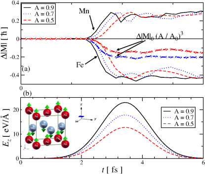
Figure 1: (Color online) Time-averaged observables evaluated in spheres of radius $0.5\text{\,}\mathrm{\SIUnitSymbolAngstrom}$ around each atom: (a) the averaged temporal variation of the spin density module $\absolutevalue{\Delta\mathbf{S}^{\mathrm{N}}(t)}=\int_{\mathcal{S}_{\mathrm{N}}^{\mathrm{R}}}\differential[3]{r}(\absolutevalue{\mathbf{s}(\mathbf{r},t)}-\absolutevalue{\mathbf{s}(\mathbf{r},0)})$ under various laser pulses for the two Fe and Mn sites; (b) the different laser pulses employed in the dynamical simulations with shape $E_{\mathrm{z}}(t)=A\cdot\sin(0.1\cdot t)\cdot\exp(-(t-5)^{2}/3)$ for t in fs. The amplitudes $A$ are in units of eV /$\mathring{A}$ (the black arrow in the inset indicates the electric field polarization direction).

In order to analyze how the quantities previously defined evolve dynamically in a real magnetic system under the action of an external electric pulse, we look at bulk FeMn. The ground state properties of this material have been already studied in the past femn1 ; femn2 , even though there is no full consensus on the magnetic structure of the ground-state, since the various theoretical results often vary with the method and approximation employed. Here we consider the anti-ferromagnetic ground-state in its fcc phase with lattice constant $a=$3.7\text{\,}\mathrm{\SIUnitSymbolAngstrom}$$ [see inset in Fig. 1(b)]. This structure represents the starting point of our dynamical evolution. We use the ALDA alda exchange-correlation functional with the Perdew and Wang Wang92 parametrization as implemented in the Octopus code Octop1 . The ground state is characterized by two localized magnetic moments over the Fe and Mn sites with a magnitude $\absolutevalue{\mathbf{S}}\simeq 0.57~{}\hbar$ computed by integrating the spin density within atom centered spheres of radius $0.5\text{\,}\mathrm{\SIUnitSymbolAngstrom}$. The amount of non collinearity is not negligible but the ratio among $m_{\mathrm{z}}$ and $m_{\mathrm{x}}$ (or $m_{\mathrm{y}}$) is always approximately $4$ and it has the tendency to increase with the distance from the atom. The $z$ component of the magnetization vector is thus locally dominant, even if over the entire simulation box it is approximately zero due to the overall anti-ferromagnetic nature of the system.

In all our calculations the system is perturbed from the initial equilibrium ground state by applying intense, spatially homogeneous, electric pulses, with duration typically between $7$ fs and $10$ fs. The pseudopotentials for both Fe and Mn employed in the calculations are fully relativistic and norm-conserving. They are generated using a multi-reference pseudo-potential (MRPP) scheme mrpp at the level implemented in APE APE ; APE2 , which evolves the valence states and the semi-core states simultaneously.

In order to analyze the spin dynamics in an anti-ferromagnetic material we need to partition the spin density so to isolate the magnetic moments and the electronic charges associated with each atomic site $N$ in the unit cell. The simplest choice consists in integrating the densities inside a sphere $\mathcal{S}_{\mathrm{N}}^{\mathrm{R}}$ of radius $R$ centered on the atomic site $N$. Thus the local spin and charge densities read respectively

$$\mathbf{S}^{\mathrm{N}}(t)=\int_{\mathcal{S}_{\mathrm{N}}^{\mathrm{R}}}\differential[3]{r}\mathbf{s}(\mathbf{r},t)\>,\>\>\>\quad Q^{\mathrm{N}}(t)=\int_{\mathcal{S}_{\mathrm{N}}^{\mathrm{R}}}\differential[3]{r}\;n(\mathbf{r},t)\>.$$ (34)

In Fig. 1(a) we show the demagnetization observed around the Fe and the Mn sites in the first $20$ fs under different laser pulses, all polarized along the $z$ direction but with different amplitudes. The demagnetization process is quite pronounced since, in all the cases, each atom loses around $60\%$ of the initial magnetization almost immediately after the action of the pulse and then it stabilizes around a different value of the magnetization vector. The demagnetization rate, instead, differs in the three cases. In particular we observe from Fig. 1(a) an initial decay rate proportional to the the cube of the laser field amplitude

$$\absolutevalue{\mathbf{S}(t_{\mathrm{in}}+\delta t)}-\absolutevalue{\mathbf{S}(t_{\mathrm{in}})}\sim-A^{3}\>,$$ (35)

where $t_{\mathrm{in}}$ is the initial time at which the laser pulse is applied, $\delta t$ is a small time step, while $A$ represents the amplitude of the applied laser pulse in $eV/\mathring{A}$. Hence the demagnetization rate increases substantially for larger excitation amplitudes. At the same time the overall magnetization loss for longer times following the laser pulse does not change significantly.

The observed magnetization dynamics, localized in the vicinity of the two atomic sites, suggests the existence of a spin density transfer mechanism among different occupied and unoccupied Kohn-Sham states. Consider now the magnetization continuity equation (15), where the velocity field has been, in first approximation, neglected. We have that the dissipative term, $-\nabla\cdot\mathcal{D}(\mathbf{r},t)$, on the right-hand of the expression, is the one driving the entire dynamics during the action of the laser pulse. This influences also the other field, $\mathbf{B}_{\mathrm{eff}}(\mathbf{r},t)$, that is modified by the local changes in the spin density gradient.

After having neglected in Eq. (15) the exchange-correlation magnetic field, $\mathbf{B}_{\mathrm{xc}}(\mathbf{r},t)$, which does not contribute to the dynamics in the ALDA, but represents only an energy barrier between the spin-up and spin-down states, we are left with the equation

$$\frac{d}{dt}\mathbf{m}(\mathbf{r},t)=-\nabla\cdot\mathcal{D}(\mathbf{r},t)+\mu_{B}\mathbf{m}(\mathbf{r},t)\times\mathbf{B}_{\mathrm{kin}}(\mathbf{r},t)\>.$$ (36)

Here we finally distinguish two contributions to the spin dynamics. The first one on the right-hand side of Eq. (36) represents a measure of the spin dissipation due to the internal charge currents flowing between the different Kohn-Sham states. This term is, by construction, responsible for effective Stoner-like excitations in real time. In fact, Stoner excitations are due, by definition, to terms in the Hamiltonian of the form $\hat{c}^{\dagger}_{k,A,\uparrow}\hat{c}_{k,B,\downarrow}$, where $A$ and $B$ label the atomic site. These excitations are local in momentum space and non-local in real space and correspond to inter-site electronic excitations, which are included into the previous spin dissipation term.

The second contribution to the dynamics is due to the torque exerted by the kinetic field, $\mathbf{B}_{\mathrm{kin}}(\mathbf{r},t)$, on the magnetization vector. Due to its dependence on the gradients of the electron density and magnetization $\mathbf{B}_{\mathrm{kin}}$ drastically changes during the action of the electric pulse. In Fig. 2(b) we compare the evolution of the $z$ component of the magnetization with its transverse component $S_{\mathrm{xy}}^{\mathrm{N}}(t)=\int_{\mathcal{S}_{\mathrm{R}}^{\mathrm{N}}}\differential[3]{r}\sqrt{s_{\mathrm{x}}(\mathbf{r},t)^{2}+s_{\mathrm{y}}(\mathbf{r},t)^{2}}$. The predominant change (loss) of on-site magnetic moment during and after the action of the laser pulse is in the $z$ component, while the magnitude of the non-collinear part of the magnetization is only slightly affected.

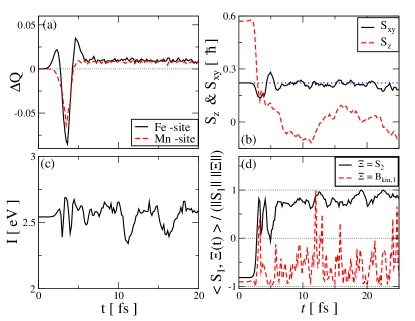
Figure 2: (Color online) Time-averaged observables evaluated in spheres of radius $0.5\text{\,}\mathrm{\SIUnitSymbolAngstrom}$ around the Fe atomic site with the same type of pulses ($A=0.7$ eV/$\mathring{A}$): (a) the averaged temporal variation of the two on-site electronic charges $\Delta Q^{\mathrm{N}}(t)=Q^{\mathrm{N}}(t)-Q^{\mathrm{N}}(t=0)$, Fe site (black curve) and Mn site (red curve); (b) the averaged temporal variation of the magnetization along the $z$ axis, $S_{z}^{\mathrm{N}}(t)$, and the non-collinear component, $S_{xy}^{\mathrm{N}}(t)$, in correspondence of the Fe site; (c) dynamical Stoner exchange parameter $I(t)$ obtained by spatial integration, $I(t)=\frac{1}{\|\mathcal{S}_{\mathrm{N}}^{\mathrm{R}}\|}\int_{\mathcal{S}_{\mathrm{N}}^{\mathrm{R}}}\differential[3]{r}I(\mathbf{r},t)$, in correspondence of the Fe site (see Eq. 38); (d) the averaged temporal variation of $F[\bm{\Xi}](t)=|\langle\mathbf{S}_{\mathrm{Fe}}(t),\bm{\Xi}(t)\rangle|/(\absolutevalue{\mathbf{S}_{\mathrm{Fe}}(t)}\cdot\absolutevalue{\bm{\Xi}(t)})$, where $\mathbf{S}_{\mathrm{Fe}}(t)$ is the on-site averaged magnetization computed within a radius $R=$1.4\text{\,}\mathrm{\SIUnitSymbolAngstrom}$$. Here $\bm{\Xi}(t)$ represents the spin calculated within the same radius over the Mn site (solid line) and the kinetic field $\mathbf{B}_{\mathrm{kin}}^{\mathrm{N}}(t)$ over the Fe site (dashed line).

It is clear that, while the component $S_{z}^{\mathrm{N}}(t)$ collapses during the action of the electric field, after that it starts to oscillate around a new averaged value . The behavior of the non-collinear component of the magnetization is instead different. After an initial bump during the action of the pulse, $S_{xy}^{\mathrm{N}}(t)$ returns to a value that is approximately equal to its initial one and then it remains constant for the rest of the time evolution. This kind of dynamics suggests the existence of different effective equations of motion for the two magnetization components. The reason for this very different dynamical behavior observed in the $S_{z}^{\mathrm{N}}$ and $S_{xy}^{\mathrm{N}}$ components lies in the fact that the Stoner excitations connect only up and down states along the spin quantization axis. In the initial ($t=0$) state the magnetic configuration of the system is, to a good level of accuracy, aligned along the $z$ axis. Hence, we would expect a pulse-driven Stoner-like excitation to mainly affect the $S_{z}^{\mathrm{N}}$ component and to a lesser degree the non-collinear $S_{xy}^{\mathrm{N}}$ magnetization.

In Fig. 2 we introduce also a time-dependent effective Stoner parameter, $I(t)$. Typically within the DFT formalism $I$ is a measure of the drag in transferring charge density between the spin-up and spin-down bands of a solid. At the level of ground-state collinear spin DFT it is therefore commonly associated with the ratio between the exchange-correlation magnetic field, $\mathbf{B}_{\mathrm{xc}}(\mathbf{r},t)$, and the local value of the magnetization density. In order to generalize this concept to the case of a non-collinear magnetic system evolving in time we note that the effective local Hamiltonian, corresponding to the magnetic energy in Eq. (III), contains together with the exchange-correlation field also a second local contribution so that we can introduce the following effective local magnetic field,

$$\mathbf{B}_{\mathrm{tot}}(\mathbf{r},t)=\mathbf{B}_{\mathrm{xc}}(\mathbf{r},t)+\mathbf{B}_{\mathrm{local}}(\mathbf{r},t)\>.$$ (37)

We use this expression to define a local Stoner vector, $\mathbf{I}(\mathbf{r},t)$, parallel to $\mathbf{B}_{\mathrm{tot}}(\mathbf{r},t)$ and normalized with respect to the amplitude of the magnetization at each spatial point

$$\mathbf{B}_{\mathrm{tot}}(\mathbf{r},t)=\mathbf{I}(\mathbf{r},t)\cdot\absolutevalue{\mathbf{m}(\mathbf{r},t)}\>.$$ (38)

Hence, similarly to Eq. (37), $\mathbf{I}(\mathbf{r},t)$ can be identified from the sum of the two separate contributions originating from the local and the exchange-correlation field, $\mathbf{I}(\mathbf{r},t)=\mathbf{I}_{\mathrm{xc}}(\mathbf{r},t)+\mathbf{I}_{\mathrm{loc.}}(\mathbf{r},t)$. In Fig. 2(c) we plot the module of the vector field $\mathbf{I}(\mathbf{r},t)$ integrated over a sphere centered at the Fe site. Its real time evolution within the first $20$ fs shows some oscillations activated by the action of the laser pulse. However, the overall change in the Stoner parameter during the evolution is not appreciable and $I(t)$ remains approximately constant throughout the entire dynamics and close to its initial value. This behaviour suggests that the initial dynamical change in the on-site $z$ component of the magnetization is mainly driven by the dissipation term $\nabla\cdot\mathcal{D}(\mathbf{r},t)$ and not due to a collapse of $I(t)$ which describes, instead, the resistance opposed by the band structure to inter-band transitions.

Fig. 2(d) shows the dynamical evolution of the function $F(t)$, which represents a measure of the normalized scalar product between the spin vector computed over the Fe site and the spin vector over the Mn site (solid line). During the action of the laser pulse $F(t)$ changes from an almost anti-ferromagnetic configuration (slightly non-collinear) to a ferromagnetic one, with the amount of spin misalignment being preserved during the process. We have seen that such an effect is determined by the Stoner excitations activated in the anti-ferromagnet by the action of the laser pulse. At longer times $F(t)$ oscillates around its new value and eventually approaches $1$, with the spin misalignment that is lifted out during the process. The dashed curve, instead, represents the evolution of $F[\bm{\Xi}](t)$, where $\bm{\Xi}(t)$ corresponds to the Fe on-site kinetic field. Within the first $5$ fs of the dynamical evolution $F(t)$ is characterized by strong fluctuations induced by the internal currents activated by the laser and its behaviour is similar to that described by the solid curve. However, after this initial phase, the evolution of $F(t)$ in the two cases appears quite different. Now, $F(t)$ strongly oscillates also after the action of the pulse inducing a torque on the magnetization vector. In practice, while the initial phase of the spin evolution is dominated by inter-band transitions activated by the action of the pulse, with consequent enhanced electronic hopping between the two atomic sites, after the action of the pulse the inter-band transitions are suppressed and the Kohn-Sham states evolve separately. The role played by the kinetic field becomes then more important inducing intra-band transitions with consequent spin relaxation over the two sites.

A further confirmation of these conclusions is provided by Fig. 3(d), where we show a comparison between the local $z$ component of the magnetization, $S_{z}^{\mathrm{Fe}}(t)$, and its module $\absolutevalue{\mathbf{S}_{\mathrm{Fe}}(t)}$. During the action of the laser both the quantities decrease even if at different rates. After this first phase $S_{z}^{\mathrm{Fe}}(t)$ starts to oscillate around its new average value, while the module remains approximately constant. These two different dynamical behaviors may be explained in terms of initial inter-band transitions followed by an intra-band dynamical relaxation mechanism with the spin that is exchanged among the different components while its module remains constant.

Similarly we find in Fig. 3(b) that the module of the exchange component $\absolutevalue{\mathbf{B}_{\mathrm{x}}^{\mathrm{Fe}}(t)}$, after the initial decay during the action of the laser remains approximately constant. In contrast the module of the local component of the kinetic field, $\absolutevalue{\mathbf{B}_{\mathrm{loc}}(t)}$, introduced in Eq. (III) appears, after the initial excitation, more oscillatory resembling the long-time dynamics of the $S_{z}^{\mathrm{Fe}}$ component. In Fig. 3(a) we compare $\absolutevalue{\mathbf{B}_{\mathrm{loc}}^{\mathrm{Fe}}}$ under the application of the pulses shown in Fig. 1(b). In all the three cases this quantity is excited by the application of the pulse, but in the second phase of the dynamical evolution it collapses to a new lower value and it starts to oscillate around it. The application of different laser amplitudes does not seem to be reflected in a clear trend of the dynamical evolution of the local field. Finally we look at panel (c) where we plot the value of $\cos\theta$, with $\theta$ being the angle formed by the spin vector $\mathbf{S}_{\mathrm{Fe}}$ (black curve), or the kinetic field $-\mathbf{B}_{\mathrm{kin}}^{\mathrm{Fe}}(t)$ (red curve) with the $z$ axis. This clearly shows, as we have already seen in Fig. 2(d), that after the application of the pulse the two vectors are highly non parallel with $\mathbf{B}_{\mathrm{kin}}$ playing a major role in the local dynamics of the spin vector.

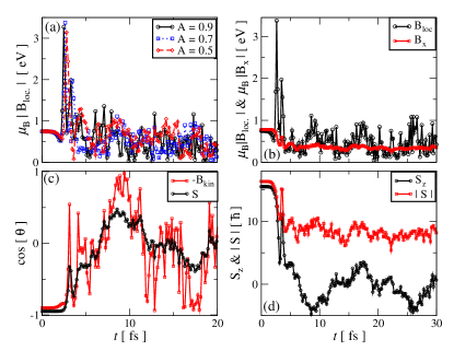
Figure 3: (Color online) Time-averaged observables evaluated in spheres of radius $1.4\text{\,}\mathrm{\SIUnitSymbolAngstrom}$ around the atomic sites: (a) The averaged temporal evolution of $\absolutevalue{\mathbf{B}_{\mathrm{loc}}^{\mathrm{Fe}}(t)}$ for different pulse amplitudes $A=0.5,0.7,0.9$ eV/Å; (b) comparison of $\absolutevalue{\mathbf{B}_{\mathrm{loc}}^{\mathrm{Fe}}(t)}$ and $\absolutevalue{\mathbf{B}_{\mathrm{x}}^{\mathrm{Fe}}(t)}$ under a single pulse with amplitude $A=$0.7\text{\,}\mathrm{e}\mathrm{V}\mathrm{/}\mathrm{\SIUnitSymbolAngstrom}$$; (c) averaged value of $\cos\theta$ during the time evolution, with $\theta$ angle formed with the $z$ axis by the $\mathbf{S}_{\mathrm{Fe}}(t)$ vector (black curve) and by the $\mathbf{B}_{\mathrm{kin}}^{\mathrm{Fe}}(t)$ vector (red curve), the pulse employed is the same of (b); (d) comparison between $\absolutevalue{\mathbf{S}_{\mathrm{Fe}}(t)}$ and $S_{z}^{\mathrm{Fe}}(t)$ during the temporal evolution, the pulse employed is the same of (b).

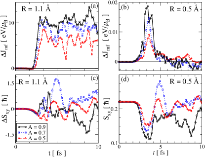
Figure 4: (Color online) Exchange coupling evaluated inside spheres of different radii $R$ centered on the Fe atomic site and of $S_{\mathrm{xy}}^{\mathrm{Fe}}$ calculated inside the same spatial regions using three different type of pulses ($A=0.7$, $A=0.9$, $A=0.5$) eV/Å. The dynamical exchange coupling here corresponds to the expression of Eq. (33): (a) the averaged temporal variation of $\Delta J_{\textrm{mf}}(t)=J_{\textrm{mf}}(t)-J_{\textrm{mf}}(t=0)$ in the first $10$ fs; (b) the averaged temporal variation of $J_{\textrm{mf}}(t)$ inside a sphere of radius $R$; (c) the averaged temporal variation of $\Delta S_{\mathrm{xy}}^{\mathrm{Fe}}(t)$ obtained by spatial integration inside a sphere of radius $R$; (d) the averaged temporal variation of the same quantity $S_{\mathrm{xy}}^{\mathrm{Fe}}(t)$ evaluated inside a sphere of radius $R$.

We can now focus our attention on the effective mean field term introduced in Eq. (32) that has the form of a spin-spin interaction. This object, a non-local function of the magnetization vector density, can effectively be the source of spin waves in the dynamical evolution of the system. The temporal evolution of the dynamical exchange parameter $J_{\mathrm{mf}}(t)$ is presented in Fig. 4 panels (a) and (b) and it appears to be strongly dependent on the laser-pulse excitation. In panel (b) it is shown that $J_{\mathrm{mf}}(t)$ follows the shape of the pulse. The value of the field is integrated within a sphere of small radius ($R=$0.5\text{\,}\mathrm{\SIUnitSymbolAngstrom}$$) around the Fe site, therefore, higher pulse amplitudes excite more the electronic system with consequent higher modification of $J_{\mathrm{mf}}$. The quantity sharply increases from its initial value and then returns close to its ground-state magnitude on the time scale of the pulse disappearence. The maximum amplitude of $J_{\mathrm{mf}}$ also scales systematically with the amplitude of the laser pulse, i.e. it increases for the more intensive pulses. The trend of $J_{\mathrm{mf}}(t)$ shown in panel (a) is very similar, the quantity is computed within a sphere of larger radius. While during the application of the pulse $J_{\mathrm{mf}}(t)$ looks strongly affected, and its growth rate scales proportionally to the pulse amplitude, after that the exchange coupling stabilizes around an average value, different in the three cases. This reflects the different amount of energy injected into the system by the three pulses.

In comparison, Figure 4 panels (c) and (d) show the evolution of the non-collinear spin function, $S_{xy}^{\mathrm{Fe}}(t)$, for the same set of simulations with increasing laser-pulse intensity. We find clear similarities during the pulse-coherent stage of the dynamics. Both $J_{\textrm{mf}}(t)$ and $S_{xy}^{\mathrm{Fe}}(t)$ follow the pulse, and their amplitudes vary with the pulse intensity. At times longer than the pulse duration the dynamics of the two objects, however, is completely different. This difference stems from the fact that the non-collinear spin component $S_{xy}^{\mathrm{N}}(t)$ is driven by two torques, as described by Eq. (32), and only a part of the second torque is related to $J_{\textrm{mf}}$. The dynamical exchange coupling shown in Fig. 4(b) is characterized by a large variation during the action of the laser pulse and it could, at least in principle, activate an out-of-equilibrium dynamics involving the non-collinear components of the two atomic spins. We will see now that this is indeed the case.

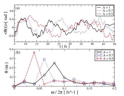
Figure 5: (Color online) Time-averaged observables evaluated in spheres of radius $0.5\text{\,}\mathrm{\SIUnitSymbolAngstrom}$ around the Fe atomic site with three different type of pulses ($A=1.0,0.7,0.5$ eV/Å): (a) the temporal variation of the angle $\theta(t)=\arccos\big(S_{z}^{\mathrm{Fe}}(t)/\absolutevalue{\mathbf{S}^{\mathrm{Fe}}}\big{missing})$ with respect to its temporal averaged value $\langle\theta(t)\rangle=\frac{\sum_{n=1}^{N}\theta(t_{n})}{N}$; (b) the Fourier transform $\mathfrak{F}(\theta)(\omega)$ where $\theta(t)$ is the angle previously defined.

Further evidence of the validity of this argument for the spin-spin exchange are provided in Fig. 5(b), where we present the Fourier transform of the angle $\theta(t)$ formed by the spin vector, $\mathbf{S}^{\mathrm{Fe}}(t)$, on the Fe site [see Eq. (34)] with the $z$ axis. In panel (a) we present the corresponding temporal evolution of $\theta(t)$ by measuring the on-site spin misalignment (Fe atom). As before we compare the results from the three different simulations with increasing pulse amplitudes. Focusing on the lowest part of the spectrum, we observe that the lowest frequency peak in the spectrum blue-shifts with increasing the pulse amplitude. Although our resolution is limited by the length of the numerically-stable time integration and we only observe one or two periods of the lowest frequency mode, it is clear that the laser pulse amplitude affects directly the energy of that spin-wave mode. This correlates with our previous observation of strongly pulse-intensity dependent effective exchange interaction $J_{\textrm{mf}}$.

In a summary, it is clear that the laser excites directly only the electronic system and this is propagated to the spin system through the consequent formation of Stoner excitations and transfer of magnetization between the two sites. However, at the same time the excitations in the electronic sub-system contribute also to the ultrafast modification of the effective inter-site EDEI $J_{\textrm{mf}}(t)$ depicted in Fig. 4(a). Certainly, the degree of laser-induced modification of this quantity is proportional to the amount of energy injected into the system by the pulse, namely to the amplitude of the applied external field. The physical interpretation of $J_{\textrm{mf}}(t)$ as a Heisenberg-like exchange parameter is further validated by the observation that the lower energy spin-wave modes follow an analogous dependence on the excitation magnitude.

V Conclusions

In conclusion, starting from the hydrodynamical formulation of the spin dynamics in the ALDA, we introduce an out-of-equilibrium non-local spin-spin interaction term and define an effective out-of-equilibrium Heisenberg-like exchange coupling. We evaluate the latter through TD-SDFT calculations by applying ultrafast external electric pulses (of duration of about 5 fs and amplitudes ranging between $A=0.5$ eV/Å and $A=1$ eV/Å) to fcc FeMn, which has a frustrated anti-ferromagnetic ground-state. These simulations show that the observed on-site demagnetization can be attributed mainly to a Stoner-like excitation activated by the action of the laser pulse. The local dynamics, at longer time, appears to be driven by an inter-site exchange coupling, $J_{\mathrm{mf}}(t)$. After a strong non-adiabatic modification during the action of the pulse the EDEI acquires a new value that remains approximately constant for the rest of the evolution. The analysis of the Fourier spectrum of the angle $\theta(t)$ formed by the on-site spin direction with the $z$ axis suggests that the laser pulse can activate spin wave excitations with a frequency that grows with the amplitude of the applied pulse and correlates also with the new value acquired by the effective exchange coupling $J_{\mathrm{mf}}$.

- (1)
- (2) M.I. Katsnelson and A.I. Lichtenstein, Phys. Rev. B 61, 8906 (2000).
- (3) M.I. Katsnelson and A.I. Lichtenstein, J. Phys.: Condens. Matter 16, 7439 (2004).
- (4) S. Lounis and P.H. Dederichs, Phys. Rev. B 82, 180404(R) (2010).
- (5) A. Jacobsson, B. Sanyal, M, Lez̆aić and S. Blügel, Phys. Rev. B 88, 134427 (2013).
- (6) A.I. Liechtenstein, M.I. Katsnelson, V.P. Antropov and V.A. Gubanov, J. Magn. Magn. Mater. 67, 65 (1987).
- (7) V.P. Antropov, J. Magn. Magn. Mater. 262, 192 (2003).
- (8) P. Bruno, Phys. Rev. Lett. 90, 087205 (2003).
- (9) A. Szilva, M. Costa, A. Bergman, L. Szunyogh, L. Nordström and O. Eriksson, Phys. Rev. Lett. 111, 127204 (2013).
- (10) K.L. Liu and S.H. Vosko, Can. J. Phys. 67, 1015 (1989).
- (11) M.A.L Marques and E.K.U. Gross in A Primer in Density Functional Theory, edited by C. Fiolhais, F. Noqueira and M. Marques, Lecture Notes in Physics Vol. 620 (Springer-Verlag, Berlin, 2003)
- (12) E.K.U. Gross and W. Kohn, Adv. Quantum Chem. 21, 255 (1990).
- (13) M. Stamenova and S. Sanvito, Phys. Rev. B 88, 104423 (2013).
- (14) J.E. Peralta, O. Hod and G.E. Scuseria, J. Chem. Theory Comput. 11, 3661 (2015).
- (15) A.V. Kimel, A. Kirilyuk and Th. Rasing Laser & photon. Rev. 1, 275 (2007).
- (16) E. Beaurepaire, J.-C. Merle, A. Daunois and J.-Y. Bigot, Phys. Rev. Lett. 76, 4250 (1996).
- (17) E. Carpene, H. Hedayat, F. Boschini and C. Dallera, Phys. Rev. B 91, 174414 (2015).
- (18) G.P. Zhang, M. Gu and S.X. Wu, J. Phys.:Condens. Matter 26, 376001 (2014).
- (19) A. Secchi et Al., Annals of Physics 333, 221 (2013).
- (20) B.Y. Mueller, A. Baral, S. Vollmar, M. Cinchetti, M. Aeschlimann, H.C. Schneider and B. Rethfeld, Phys. Rev. Lett. 111, 167204 (2013).
- (21) P. Elliott, T. Müller, J.K. Dewhurst, S. Sharma and E.K.U. Gross, Sci. Rep. 6, 38911 (2016).
- (22) G.P. Zhang, M.S. Si, Y.H. Bai and T.F. George, J. Phys.: Condens. Matter 27, 206003 (2015).
- (23) T. Takabayasi, Prog. Theor. Phys. 14, 283 (1955).
- (24) V.P. Antropov, J. Appl. Phys. 97, 10A704 (2005).
- (25) M.I. Katsnelson and V.P. Antropov, Phys. Rev. B 67, 140406(R) (2003).
- (26) V. Antropov, M.I. Katsnelson, B.N. Harmon, M. van Schilfgaarde and D. Kusnezov, Phys. Rev. B 54, 1019 (1996).
- (27) J. Simoni, M. Stamenova and S. Sanvito, Phys. Rev. B 95, 024412 (2017).
- (28) K. Capelle, G. Vignale and B.L. Györffy, Phys. Rev. Lett. 87, 206403 (2001).
- (29) M. Ekholm and I.A. Abrikosov, Phys. Rev. B 84, 104423 (2011).
- (30) C. Grazioli, D. Alfé, S.R. Krishnakumar, S.S. Gupta et Al., Phys. Rev. Lett. 95, 117201 (2005).
- (31) K. Yabana and G.F. Bertsch, Phys. Rev. B 54, 4484 (1996).
- (32) J. Zhu, X.W. Wang and S.G. Louie, Phys. Rev. B 45, 8887 (1992).
- (33) A. Castro, H. Appel, M. Oliveira, C.A. Rozzi, et al., Phys. Stat. Sol. B 243, 2465 (2006).
- (34) C.L. Reis, J.M. Pacheco and J.L. Martins, Phys. Rev. B 68, 155111 (2003).
- (35) M. J. T. Oliveira and F. Nogueira, Comp. Phys. Comm. 178, 524 (2008).
- (36) M.A.L. Marques, M.J.T. Oliveira and T. Burnus, Comp. Phys. Comm., 183, 2272 (2012).