Correlated Multivariate Poisson Processes and Extreme Measures

Abstract

Multivariate Poisson processes have many important applications in Insurance, Finance, and many other areas of Applied Probability. In this paper we study the backward simulation approach to modelling multivariate Poisson processes and analyze the connection to the extreme measures describing the joint distribution of the processes at the terminal simulation time.

1 Introduction

Analysis and simulation of dependent Poisson processes is an important problem having many applications in Insurance, Finance, Operational Risk modelling and many other areas (see Aue and Kalkbrener, (2006), Böcker and Klüppelberg, (2010), Chavez-Demoulin et al., (2006), Duch et al., (2014), Embrechts and Puccetti, (2006), Panjer, (2006), Shevchenko, (2011) and references therein). In the modelling of multivariate Poisson processes, the specification of the dependence structure is an intriguing problem. In some applications, such as Operational Risk, the realized correlations between components of multivariate Poisson Processes exhibit negative correlations that cannot be ignored, as exemplified in the correlation matrix below.

$$\begin{bmatrix}1.0&0.14&0.29&0.32&0.15&0.16&0.03\\ 0.14&1.0&0.55&-0.12&0.49&0.52&-0.16\\ 0.29&0.55&1.0&0.11&0.27&0.17&-0.31\\ 0.32&-0.12&0.11&1.0&-0.12&-0.23&0.19\\ 0.15&0.49&0.27&-0.12&1.0&0.49&-0.17\\ 0.16&0.52&0.17&-0.23&0.49&1.0&-0.02\\ 0.03&-0.16&-0.31&0.19&-0.17&-0.02&1.0\\ \end{bmatrix}$$

In the literature, several different bivariate processes with Poisson marginal distributions are available for applications in actuarial science and quantitative risk management. One of the most popular models is the common shock model Lindskog and McNeil, (2001) where several common Poisson processes drive the dependence between the components of the multivariate Poisson process. The resulting correlation structure is time invariant and cannot exhibit negative correlations in this case.

An alternative, more flexible approach to this problem is based on the Backward Simulation (BS) introduced in Kreinin, (2016) for the bivariate Poisson processes. The BS of correlated Poisson processes and an approach to the calibration problem using transformations of Gaussian variables was proposed in Duch et al., (2014). In Kreinin, (2016), the idea of BS was extended to the class of multivariate processes containing both Poisson and Wiener components. It was also proved that the linear time structure of correlations is observed both in the Poisson and the Poisson-Wiener model. Further steps in the bivariate case were proposed in Bae and Kreinin, (2017) where the BS was combined with copula functions. This method allows one to extend the correlation pattern by using the Marshall-Olkin type copula functions that are simple to simulate.

In this paper, we continue the analysis and development of the BS method for the class of multivariate Poisson processes. By the multivariate Poisson process, we understand any vector-valued process such that all its components are (single-dimensional) Poisson processes. The idea of our approach is to use the relationship between the extreme measures describing the joint distribution with maximal or minimal correlation coefficient of the components of the multivariate process at the terminal simulation time and the time structure of correlations. We describe the class of admissible correlation structures given parameters of the marginal Poisson processes and exploit convex combinations of the extreme measures to represent the multivariate Poisson process with given correlations of the components. We believe that our approach can simplify the solution to the calibration problem and extend the variety of the correlation patterns of the multivariate Poisson processes.

There is a connection between our problem and the Optimal Transport literature (see Villani, (2008) for a general overview of the area and Rachev and Rüschendorf, 1998a ; Rachev and Rüschendorf, 1998b for a more probabilistic focus). Our computation of the extreme measures at the terminal simulation time can be viewed as a solution to a special multi-objective Monge-Kantorovich Mass Transportation Problem (MKP), with quadratic cost functions. However, this connection is not discussed in the present paper. In this paper, we are mainly concerned with the construction of the multivariate Poisson processes.

The rest of the paper is organized as follows. In Section 2 we begin by discussing the background and motivation for the 2-dimensional problem. We introduce extreme measures and generalize the results of the bivariate problem to higher dimensions in Section 3. In Section 4 we describe a general algorithm for the computation of the joint distribution of the extreme measures. Section 5 is concerned with the calibration problem. We discuss the simulation problem in Section 6 and propose a Forward-Backward extension of the BS method. The paper is concluded with some directions for future research in Section 7.

2 Extreme Measures and Monotonicity of the Joint Distributions

We begin with a description of the Common Shock Model (CSM) Lindskog and McNeil, (2001) and the motivation of the approach proposed in Duch et al., (2014). Afterwards, we discuss the results obtained in Kreinin, (2016) for the case of two Poisson processes and describe the computation of the extreme measures in the case $J=2$.

The CSM has become very popular within actuarial applications as well as in Operational Risk modeling Powojowski et al., (2002). This model is based on the following idea. Suppose we want to construct two dependent Poisson processes. Consider three independent Poisson processes $\nu^{(1)}_{t}$, $\nu^{(2)}_{t}$, $\nu^{(3)}_{t}$ with the intensities $\lambda_{1}$, $\lambda_{2}$, $\lambda_{3}$. Let $N^{(1)}_{t}=\nu^{(1)}_{t}+\nu^{(2)}_{t}$ and $N^{(2)}_{t}=\nu^{(3)}_{t}+\nu^{(2)}_{t}$, which are also Poisson processes, formed by the superposition operation. Then, the Poisson processes $N^{(1)}_{t}$ and $N^{(2)}_{t}$ are dependent with the Pearson correlation coefficient

$$\rho(N^{(1)}_{t},N^{(2)}_{t})=\frac{\lambda_{2}}{\sqrt{(\lambda_{1}+\lambda_{2})(\lambda_{2}+\lambda_{3})}}.$$

Clearly, the correlation coefficient can only be positive.

A more advanced approach to the construction of negatively correlated Poisson processes is based on the idea of the backward simulation of the Poisson processes Kreinin, (2016). The conditional distribution of the arrival moments of a Poisson process, conditional on the value of the process at the terminal simulation time, $T$, is uniform. Then, using a joint distribution maximizing or minimizing correlation between the components at time, $T$, one can construct a Poisson process with a linear time structure of correlations in the interval $t\in[0,T]$. Thus, the problem of constructing the $2$-dimensional Poisson process with the extreme correlation of the components at time $T$ is reduced to that of random variables having Poisson distributions with the parameters $\lambda T$ and $\mu T$, where $\lambda$ and $\mu$ are parameters of the processes. It is not difficult to see that maximization (minimization) of the correlation coefficient of two random variables (r.v.), $X$ and $Y$, given their marginal distributions, is equivalent to maximization (minimization) of $\mathbb{E}[XY]$, if the r.v. have finite first and second moments and positive variances.

The admissible range of the correlation coefficients can be computed using the Extreme Joint Distributions (EJD) Theorem in Kreinin, (2016) (see Theorem 2.2 in this section). The key statement, the characterization of the EJDs, is equivalent to the Frechet-Hoeffding theorem Fréchet, (1960) for distributions on the positive quadrant of the two-dimensional lattice, ${\mathbb{Z}}^{(2)}_{+}=\{(i,j):i,j=0,1,2,\dots\}$. However, taking into account the numerical aspect of the problem, we prefer to use equations, derived in Kreinin, (2016), written in terms of the probability density function, not in terms of the cumulative distribution function. Given marginal distributions of the non-negative, integer-valued random variables $X_{1}$ and $X_{2}$, with finite first and second moments, there exist two joint distributions, $F^{*}(i,j)$ and $F^{**}(i,j)$ minimizing and maximizing the correlation, $\rho=\text{corr}(X_{1},X_{2})$, respectively.

Definition 2.1.

The probability measures corresponding to the joint distributions $F^{*}$ and $F^{**}$ are called extreme probability measures.

The EJD theorem in Kreinin, (2016) allows one to construct the extreme measures $p^{*}$ and $p^{**}$, given marginal distributions of $X_{1}$ and $X_{2}$, with the minimal negative correlation $\rho^{*}$ and maximal positive correlation $\rho^{**}$, respectively. The extreme correlation coefficient uniquely defines the extreme measure.

Given a probability measure, $p$, corresponding to the joint distribution of the vector $(X_{1},X_{2})$ on ${\mathbb{Z}}^{(2)}_{+}$ we define a functional $f_{\rho}(p)=\text{corr}(X_{1},X_{2})$. Then we have $\rho^{*}=f_{\rho}(p^{*}),\text{and}\,\,\rho^{**}=f_{\rho}(p^{**})$. This functional $f_{\rho}$ preserves the convex combination property. Indeed, taking a convex combination of the extreme measures, $p=\theta p^{*}+(1-\theta)p^{**}$, $(0\leq\theta\leq 1)$, we obtain

$$f_{\rho}(p)=\theta f_{\rho}(p^{*})+(1-\theta)f_{\rho}(p^{**}).$$ (1)

Thus, for any $\rho\in[\rho^{*},\rho^{**}]$, we can find a probability measure $p$ for a joint distribution of the vector $(X_{1},X_{2})$ such that $f_{\rho}(p)=\text{corr}(X_{1},X_{2})=\rho$ and $p$ has the required marginal distributions for $X_{1}$ and $X_{2}$.

Connection to Optimization Problem

Computation of the extreme measures in the case $J=2$ was accomplished in Kreinin, (2016) using a very efficient EJD algorithm having linear complexity with respect to the number of points in the support of the marginal distributions. It is interesting to note that this algorithm is applicable to a more general class of linear optimization problems on a lattice. In the case $J>2$, the corresponding optimization problem becomes multi-objective with $M=J(J-1)/2$ objective functions. Let us first recall the case $J=2$.

Let $(X_{1},X_{2})$ be a random vector with support $\mathbb{Z}^{(2)}_{+}$ and given marginal probabilities ${\mathbb{P}}(X_{1}=i)=P_{1}(i)$ and ${\mathbb{P}}(X_{2}=j)=P_{2}(j)$. Denote

$$h(p):=\mathbb{E}[X_{1}X_{2}]=\sum^{\infty}_{i=0}\sum^{\infty}_{j=0}ij\,p(i,j)$$

where $p(i,j)={\mathbb{P}}(X_{1}=i,X_{2}=j)$. The measure $p^{**}$ is the solution to the problem $h(p)\to\max$ with the constraints shown below in (2) on the marginal distributions of $p^{**}$. Similarly, the extreme measure $p^{*}$ is the solution to the optimization problem $h(p)\to\min$ with the same constraints Kreinin, (2016). For the sake of brevity, we write these two problems as

$$\quad h(p)\rightarrow\operatorname*{extr}$$ (2)

subject to

$$\quad\sum^{\infty}_{j=0}p(i,j)=P_{1}(i),\quad i=0,1,\dots$$

$$\quad\sum^{\infty}_{i=0}p(i,j)=P_{2}(j),\quad j=0,1,\dots$$

$$\quad p(i,j)\geq 0\quad i,j=0,1,2,\dots$$

where $\sum_{i=0}^{\infty}\limits P_{1}(i)=\sum_{j=0}^{\infty}\limits P_{2}(j)=1$. The symbol $\operatorname*{extr}$ denotes $\max$ in the case of measure $p^{**}$ and $\min$ in the case of $p^{*}$. It is not difficult to see that Problem (2) is infinite dimensional; its numerical solution requires construction of the compact subset of the lattice for the computation of the approximate solution Kreinin, (2016).

A solution to the infinite dimensional optimization problem (2) is the joint distribution describing one of the extreme measures, given the marginal distributions of the random variables. The EJD algorithm discussed in Kreinin, (2016) allows one to find a unique solution to the problem to any user specified accuracy. Taking the marginal distributions to be Poissonian, we find the extreme measures, $p^{*}$ and $p^{**}$, describing the joint distribution of the processes, $N_{T}=(N^{(1)}_{T},N^{(2)}_{T})$ with the extreme correlation of the components at time $T$.

The convex combination of these measures can be calibrated to the desired value of the correlation coefficient, $\rho$. Then, applying the BS method we obtain the sample paths of the processes. Note that the EJD algorithm is applicable to a more general class of linear optimization problems: there is no need to assume normalization conditions as long as $P_{1}(i)\geq 0$ and $P_{2}(j)\geq 0$ for all $i\geq 0$ and $j\geq 0$ and these functions are integrable: $\sum_{i=0}^{\infty}\limits P_{1}(i)<\infty$ and $\sum_{j=0}^{\infty}\limits P_{2}(j)<\infty$.

Monotone Distributions

Extreme measures are closely connected to the monotone distributions in the case $J=2$. It was proved in Kreinin, (2016) that the joint distribution is comonotone in the case of maximal correlation and antimonotone in the case of minimal (negative) correlation. Let us review the properties of extreme measures used in what follows.

Consider a set $\mathcal{S}=\{s_{n}\}_{n\geq 0}$, where $s_{n}=(x_{n},y_{n})\in\mathbb{R}^{2}$. Define the two subsets $\mathcal{R}_{+}=\{(x,y)\in\mathbb{R}^{2}:x\cdot y\geq 0\}\qquad\text{and}\qquad\mathcal{R}_{-}=\{(x,y)\in\mathbb{R}^{2}:x\cdot y\leq 0\}$.

Definition 2.2.

A set $\mathcal{S}=\{s_{n}\}_{n\geq 0}\subset\mathbb{R}^{2}$ is comonotone if $\forall\,i,j$, $s_{i}-s_{j}\in\mathcal{R}_{+}$. Similarly, $\mathcal{S}$ is antimonotone if $\forall\,i,j$, $s_{i}-s_{j}\in\mathcal{R}_{-}$.

Definition 2.3 (Monotone distributions).

We say that a distribution $P$ is comonotone (antimonotone) if its support is a comonotone (antimonotone) set.

It is also useful to recall the following classical statement on monotone sequences of real numbers, usually attributed to Hardy.

Consider two vectors $x\in\mathbb{R}^{N}$ and $y\in\mathbb{R}^{N}$. Their inner product is

$$\langle x,y\rangle:=\sum^{N}_{k=1}x_{k}y_{k}$$

Denote by $\mathfrak{S}_{N}$ the set of all permutations of $N$ elements.

Lemma 2.1.

For any monotonically increasing sequence, $x_{1}\leq x_{2}\leq\dots\leq x_{N}$ and a vector $y\in\mathbb{R}^{N}$, there exist permutations $\pi_{+}$ and $\pi_{-}$ solving the optimization problems

$$\langle x,\pi_{+}y\rangle=\max_{\pi\in\mathfrak{S}_{N}}\langle x,\pi y\rangle$$

and

$$\langle x,\pi_{-}y\rangle=\min_{\pi\in\mathfrak{S}_{N}}\langle x,\pi y\rangle$$

The permutations $\pi_{+}$ and $\pi_{-}$ sort vectors in ascending and descending order, respectively.

Lemma 2.1 motivates the introduction of monotone distributions in the $2$-dimensional case.

Theorem 2.2 (Kreinin, (2016)).

The joint distribution $p^{**}$ for $X_{1}$ and $X_{2}$ having maximal positive correlation coefficient $\rho^{**}$, given marginal distributions $F_{1}(i)$ and $F_{2}(j)$, is comonotone. The probabilities $p^{**}(i,j)=\mathbb{P}(X_{1}=i,X_{2}=j)$ satisfy the equation

$$p^{**}(i,j) =[\min(F_{1}(i),F_{2}(j))-\max(F_{1}(i-1),F_{2}(j-1))]^{+}\quad i,j=0,1,2,\dots$$ (3)

where $[\,x\,]^{+}=\max(x,0)$ and $F_{i}(\cdot)$ denote the marginal CDFs, with $F_{i}(-1)=0$.

The joint distribution $p^{*}$ for $X_{1}$ and $X_{2}$ having minimal negative correlation coefficient $\rho^{*}$ is antimonotone. In this case

$$p^{*}(i,j)=[\min(F_{1}(i),\bar{F}_{2}(j-1))-\max(F_{1}(i-1),\bar{F}_{2}(j))]^{+}\quad i,j=0,1,2,\dots$$ (4)

where $\bar{F}_{i}(j)=1-F_{i}(j)$ and $\bar{F}_{i}(-1)=1$.

Theorem 2.2 is equivalent to the Frechet theorem in the case the marginal distributions are discrete.

The case of the Poisson marginal distributions is a particular case of Theorem 2.2. This result is applicable to much more general classes of distributions. In particular, one can describe the joint probabilities corresponding to $p^{*}$ and $p^{**}$ in the case the components of the vector have a negative binomial distribution. The EJD algorithm for computation of the joint probabilities is also applicable to more general cases. If both marginal distributions have finite second moments, the joint distribution can be approximated to any user specified accuracy.

3 Extreme Measures in Higher Dimensions

Let us now generalize the main result, Theorem 2.2, discussed in Section 2. We consider a random vector $\vec{X}=(X_{1},\dots,X_{J})$ on a positive quadrant of the $J$-dimensional lattice, ${\mathbb{Z}}^{(J)}_{+}$. Each coordinate of $\vec{X}$ has a discrete distribution with the support $\mathbb{Z}_{+}$. We also assume that each random variable $X_{k}$, $k=1,2,\dots,J$, has finite second moment and its variance is positive. In this case, the correlation coefficients, $\rho_{k,l}=\text{corr}(X_{k},X_{l})$, are defined for all $1\leq k\leq l\leq J$. We denote the marginal distribution of the r.v. $X_{k}$ by $F_{k}$:

$$F_{k}(i)=\mathbb{P}(X_{k}\leq i),\quad i\in\mathbb{Z}_{+};\quad k=1,2,\dots,J.$$

Let us now define the extreme measures on the $J$-dimensional lattice. If $J=2$, the extreme measures are described by the joint distribution maximizing and minimizing the correlation coefficient of $X_{1}$ and $X_{2}$; the corresponding probability density functions satisfy Theorem 2.2. If the number of components $J\geq 3$, the definition of the extreme measure is less obvious.

Denote the (joint) distribution function of $\vec{X}$ by $F(\vec{i})$: $F(i_{1},i_{2},\dots,i_{J})={\mathbb{P}}(X_{1}\leq i_{1},X_{2}\leq i_{2},\dots,X_{J}\leq i_{J})$ and the corresponding probability density function by $p(\vec{i})$. By $p_{k,l}(i_{k},i_{l})$ we denote the probability density function of the $2$-dimensional projection, $(X_{k},X_{l})$ of $\vec{X}$, $(1\leq k<l\leq J)$:

$$p_{k,l}(i_{k},i_{l})=P(X_{k}=i_{k},X_{l}=i_{l})$$

Definition 3.1.

We say that the density $p(\vec{i})$,

$$p(i_{1},\dots,i_{J})=\mathbb{P}(X_{1}=i_{1},\dots,X_{J}=i_{J}),\quad i_{k}\in\mathbb{Z}_{+},\quad k=1,2,\dots,J$$

determines an extreme measure on the $J$-dimensional lattice if and only if for all $k$ and $l$, $(1\leq k\leq l\leq J)$, the associated density $p_{k,l}$ determines an extreme measure on ${\mathbb{Z}}^{(2)}_{+}$ in the sense of Definition 2.1.

Our goal is to describe the extreme measures given the marginal distributions, $F_{k}$, and compute the associated extreme correlation matrices, $\mathbf{\rho}=[\rho_{k,l}]$. Let us first find the number of extreme measures.

Lemma 3.1.

For any given set of marginal distributions, $F_{k}$, on $\mathbb{Z_{+}}$ $(k=1,2,\dots,J)$ the number of extreme measures is $N=2^{J-1}$.

Proof.

The proof of Lemma 3.1 for $J=2$ is obvious. Let us prove it for $J\geq 3$. For each $2$-dimensional projection $(X_{k},X_{l})$, the corresponding joint distribution should be either comonotone or antimonotone. Take the first r.v, $X_{1}$, and form the first group of random variables from the set $X_{2}$, $X_{3}$, $\dots,X_{J}$, that are comonotone with $X_{1}$. Denote the number of comonotone r.v., by $J_{c}$. The number of r.v. antimonotone with $X_{1}$, satisfies

$$J_{a}=J-1-J_{c}.$$

The total number of partitions of the number $J-1$ in the additive form, $J-1=J_{a}+J_{c}$, is $N=2^{J-1}$. Clearly, $N$ does not depend on the choice of the first r.v. ∎

Let us now introduce the monotonicity structure of the extreme measures. Take the first r.v., $X_{1}$ and consider the r.v. $X_{2}$, $X_{3}$, $\dots X_{J}$. Define the vector of binary variables $\vec{e^{n}}=(e_{1},e_{2},\dots,e_{J})$ such that $e_{1}=0$, and for $j=2,3,\dots,J$, $n=1,\dots,N$.

$$e_{j}=\begin{cases}1,&\text{if $X_{1}$ and $X_{j}$ are antimonotone,}\cr 0,&\text{if $X_{1}$ and $X_{j}$ are comonotone.}\cr\end{cases}$$

We call $\vec{e^{n}}$ the monotonicity vector corresponding to the $n$-th extreme measure; its components are called monotonicity indicators. Figure 1 illustrates this concept. In this example, all coordinates but the last are comonotone with the first r.v., $X_{1}$. The last coordinate, $X_{J}$ is antimonotone. The monotonicity indicators in this case are $e_{k}=0$, for $k=1,2,\dots,J-1$, and $e_{J}=1$.

Figure 1: Monotonicity structure of an extreme measure. Each distribution is represented by an arrow having unit length. All arrows associated with $X_{2}$, $\dots,X_{J-1}$ are oriented in the same direction as the arrow representing $X_{1}$. The last arrow pointing in the opposite direction indicates antimonotonicity of the random variables $X_{1}$ and $X_{J}$. The monotonicity structure on the right has all of its arrows reversed compared to that on the left. However, note that they both represent the same monotonicity structure.

Optimization Problem: $J\geq 3$.

Since each $2$-dimensional projection of the random vector $\vec{X}$ is associated with an extreme measure, the optimization problem in this case is multiobjective. The number of optimization criteria is $M=J(J-1)/2$, one for each pair of r.v.s $(X_{i},X_{j}),\,\,\,1\leq i<j\leq J.$ The number of constraints is equal to the number of marginal distributions, $J$. The variables in this problem are the probabilities

$$p(\vec{i})={\mathbb{P}}(X_{1}=i_{1},X_{2}=i_{2},\dots,X_{J}=i_{J}),\quad i_{j}\in\mathbb{Z_{+}},$$

and, therefore, must satisfy the inequalities $0\leq p(\vec{i})\leq 1$.

Let us define the set of integers

$$\mathcal{I}_{k}=\{j:1\leq j\leq J,\quad j\neq k,\}$$

and

$$\mathcal{I}_{k,l}=\{j:1\leq j\leq J,\quad j\neq k,\quad j\neq l\}.$$

Then the marginal probabilities, $P_{k}(i_{k})$, can be written as

$$p_{k}(i_{k})=\mathbb{P}(X_{k}=i_{k})=\sum_{j\in\mathcal{I}_{k}}\sum_{i_{j}=0}^{\infty}p(i_{1},\dots,i_{J}),\quad i_{k}\in{\mathbb{Z}}_{+}.$$

The probabilities of the $2$-dimensional projections

$$p_{k,l}(i_{k},i_{l})={\mathbb{P}}(X_{k}=i_{k},X_{l}=i_{l}),\quad k,l=1,2,\dots,J,~{}k\neq l,~{}k,l\in{\mathbb{Z}}_{+},$$

are computed as

$$p_{k,l}(i_{k},i_{l})=\sum_{j\in\mathcal{I}_{k,l}}\sum_{i_{j}=0}^{\infty}p(i_{1},\dots,i_{J}).$$

Similarly, the objective functions, $h_{k,l}(p)=\mathbb{E}[X_{k}X_{l}]$, take the form

$$h_{k,l}(p)=\sum_{i_{k}=1}^{\infty}\sum_{i_{l}=1}^{\infty}i_{k}i_{l}p_{k,l}(i_{k},i_{l}),\quad 1\leq k<l\leq J.$$

The optimization problem can then be written as

$$h_{k,l}(p)\rightarrow\,\,\textrm{extr}\quad 1\leq k<l\leq J,$$ (5)

subject to

$$\sum_{j\in\mathcal{I}_{k}}\sum_{i_{j}=0}^{\infty}p(i_{1},\dots,i_{J}),=P_{k}(i_{k})\quad i_{k}\in{\mathbb{Z}}_{+},\quad k=1,\dots,J$$

$$p\,(i_{1},\dots,i_{J})\geq 0$$

where $P_{j}(\cdot)$ are given marginal probabilities $(j=1,2,\dots,J)$.

The main theorem

Let us now formulate the main result of the paper. It is convenient to introduce the following notation.

$$\tilde{F}_{j}(i_{j},e_{j})=\begin{cases}F_{j}(i_{j})\quad&\text{if}\,\,\,e_{j}=0\\ 1-F_{j}(i_{j})\quad&\text{if}\,\,\,e_{j}=1\end{cases}$$ (6)

where the marginal distributions, $F_{j}(\cdot)$, satisfy

$$F_{j}(i_{l})=\sum_{i_{k}=0}^{i_{l}}P_{j}(i_{k})$$

Theorem 3.2 (Extreme Joint Distributions in Higher Dimensions).

Given marginal distributions $F_{1}$, $F_{2}$, $\dots F_{J}$ on ${\mathbb{Z}}_{+}$ and a binary vector $\vec{e^{n}}$, the extreme measure with the monotonicity structure $\vec{e^{n}}$ is defined by the probabilities

$$p^{\vec{e^{n}}}(\vec{i})=\big{[}\min(\tilde{F}_{1} (i_{1}-e_{1};e_{1}),\dots,\tilde{F}_{J}(i_{J}-e_{J};e_{J}))$$ (7)

$$-\max(\tilde{F}_{1}(i_{1}+(e_{1}-1);e_{1}),\dots,\tilde{F}_{J}(i_{J}+(e_{J}-1);e_{J}))\big{]}^{+}$$

Proof.

We give a sketch of the proof here for the general case $J\geq 2$. A more complete proof for the case $J=2$ is given in Kreinin, (2016).

Let us first show that, if $J=2$, then Equation (7) is equivalent to (3), in the case of maximal correlation, and to (4), in the case of minimal correlation. Indeed, in the first case, the distributions of $X_{1}$ and $X_{2}$ must be comonotone. Hence, $e_{1}=e_{2}=0$ and $\tilde{F}_{k}(i,e_{k})=F_{k}(i)$ for $k=1$ and 2 and all $i\geq 0$. In the antimonotone case, $e_{1}=0$, but $e_{2}=1$. Thus, $\tilde{F}_{1}(i,e_{1})=F_{1}(i)$, but $\tilde{F}_{2}(i,e_{2})=1-F_{2}(i-1)$ for all $i\geq 0$. Therefore, Equation (7) is equivalent to (3) and (4).

Let us now consider the general case, $J\geq 3$. There are two groups of the coordinates of $\vec{X}$: comonotone and antimonotone. Denote their indices by

$$\mathcal{I_{C}}=\{j:e_{j}=0\}\,\,\,\text{and}\,\,\,\mathcal{I_{A}}=\{j:e_{j}=1\}.$$

Let us now generate a large sample from the distribution $p^{\vec{e}}$ and sort them in the ascending order with respect to the first coordinate. It was shown in Kreinin, (2016) that, after sorting, the comonotone coordinates of $\vec{X}$ will be permuted in the ascending order while the antimonotone coordinates will be permuted in the descending order.

Suppose that the indices $1=k_{1}<k_{2}<k_{3}<\dots<k_{C}$ belong to $\mathcal{I_{C}}$ and the complimentary set of indices is $\mathcal{I_{A}}=\{l_{1},l_{2},\dots,l_{A}\}$. A permuted sample is represented in (8).

$$X_{1} :\overbrace{0,\dots,0}^{N_{1}(0)},\dots,\overbrace{i-1,\dots,i-1}^{N_{1}(i-1)},\,\,\,\overbrace{i,i,\dots,i}^{N_{1}(i)},\dots\overbrace{k,k\dots,k}^{N_{1}(k)},\dots$$

$$X_{\,k_{2}} :\underbrace{0,0,\dots,0}_{N_{k_{2}}(0)},\dots,\underbrace{i-1,\dots,i-1}_{N_{k_{2}}(i-1)},\,\,\underbrace{i,\dots,i}_{N_{k_{2}}(i)},\,\,\dots,$$

$$\hskip 120.92421pt\vdots$$ (8)

$$X_{\,l_{A}} :\dots\underbrace{k,k,\dots,k,}_{N_{\,l_{A}}(k)}\underbrace{k-1,\dots,k-1}_{N_{\,l_{A}}(k-1)},\dots\underbrace{2,2,2,\dots 2}_{N_{\,l_{A}}(2)},\dots$$

where $N_{k}(m)$ denotes the number of realizations of $m$ in the $k$th coordinate, $X_{k}$, of $\vec{X}$. The first position, $I_{k}^{\,C}(m)$, where the number $m$ appears in the sorted sample of the r.v. $X_{k}$ is

$$I_{k}^{\,C}(m)=1+\sum_{i=0}^{m-1}N_{k}(i),\quad k\in\mathcal{I_{C}}.$$

The last position, $E_{k}^{\,C}(m)$, where the number $m$ appears in the sorted sample of the r.v. $X_{k}$ is

$$E_{k}^{\,C}(m)=\sum_{i=0}^{m}N_{k}(i),\quad k\in\mathcal{I_{C}}.$$

As the sample size $N_{S}\to\infty$, we have

$$\lim_{N_{S}\to\infty}\frac{N_{k}(m)}{N_{S}}=p_{k}(m)\quad\textbf{a.s.}$$ (9)

Therefore, for $k\in\mathcal{I_{C}}$

$$\lim_{N_{S}\to\infty}\frac{I_{k}^{\,C}(m)}{N_{S}}=F_{k}(m-1)\quad\textbf{a.s.}.$$ (10)

and

$$\lim_{N_{S}\to\infty}\frac{E_{k}^{\,C}(m)}{N_{S}}=F_{k}(m)\quad\textbf{a.s.}.$$ (11)

In the case of the group of antimonotone coordinates, $l\in\mathcal{I_{A}}$, the first index, $I_{l}^{\,A}(m)$, where a number $m$ appears in the sorted sample of the r.v. $X_{l}$ is

$$I_{l}^{\,A}(m)=1+N_{S}-\sum_{i=0}^{m}N_{l}(i),\quad l\in\mathcal{I_{A}}.$$

The last position, $E_{l}^{\,A}(m)$, where a number $m$ appears in the sorted sample of the r.v. $X_{l}$ is

$$E_{l}^{\,A}(m)=N_{S}-\sum_{i=0}^{m-1}N_{l}(i),\quad l\in\mathcal{I_{A}}.$$

As $N_{S}\to\infty$, we have for $l\in\mathcal{I_{A}}$

$$\lim_{N_{S}\to\infty}\frac{I_{l}^{\,A}(m)}{N_{S}}=1-F_{l}(m)\quad\textbf{a.s.}.$$ (12)

and

$$\lim_{N_{S}\to\infty}\frac{E_{l}^{\,A}(m)}{N_{S}}=1-F_{l}(m-1)\quad\textbf{a.s.}.Theempiricalmeasureoftheevent$$ (13)

$$\{\vec{X}=\vec{i}\}=\Big{\{}\bigcap_{k\in\mathcal{I_{C}}}\{X_{k}=i_{k}\}\Big{\}}\,\bigcap\Big{\{}\bigcap_{l\in\mathcal{I_{A}}}\{X_{l}=i_{l}\}\Big{\}}$$

is $\mathbf{m_{N_{S}}}(\{\vec{X}=\vec{i}\})$, which coincides with that of the intersection of the intervals

$$\Big{\{}\bigcap_{k\in\mathcal{I_{C}}}[I_{k}^{\,C}(i_{k}),E_{k}^{\,C}(i_{k})]\Big{\}}\bigcap\Big{\{}\bigcap_{l\in\mathcal{I_{A}}}[I_{l}^{\,A}(i_{l}),E_{l}^{\,A}(i_{l})]\Big{\}}$$

The latter can be written as follows. The right end of the intersection of the intervals is

$$\mathcal{R}=\min\Big{(}\min_{k\in\mathcal{I_{C}}}(E_{k}^{\,C}(i_{k})),\min_{l\in\mathcal{I_{A}}}(E_{l}^{\,C}(i_{l}))\Big{)}$$

and the left end is

$$\mathcal{L}=\max\Big{(}\max_{k\in\mathcal{I_{C}}}(I_{k}^{\,C}(i_{k})),\max_{l\in\mathcal{I_{A}}}(I_{l}^{\,C}(i_{l}))\Big{)}$$

Then we obtain

$$\mathbf{\mu_{N_{S}}}(\{\vec{X}=\vec{i}\}=\frac{(\mathcal{R}-\mathcal{L})^{+}}{N_{S}}$$

Note that the length of the intersection of intervals is $0$ in the case $\mathcal{R}\leq\mathcal{L}$. As $N_{S}\to\infty$, we obtain from Equations (10)–(13)

$$\lim_{N_{S}\to\infty}\mathbf{\mu_{N_{S}}}(\{\vec{X}=\vec{i}\}=\big{[}\min( \tilde{F}_{1}(i_{1}-e_{1};e_{1}),\dots,\tilde{F}_{J}(i_{J}-e_{J};e_{J}))$$

$$- \max(\tilde{F}_{1}(i_{1}+(e_{1}-1);e_{1}),\dots,\tilde{F}_{J}(i_{J}+(e_{J}-1)\big{]}^{+}.$$

Finally, note

$$\lim_{\,N_{S}\to\infty}\mathbf{\mu_{\,N_{S}}}(\{\vec{X}=\vec{i}\}=p^{\,\vec{e}}(\vec{X}=\vec{i})\quad\textbf{a.s.}$$

Thus (7) is derived and the theorem is proved. ∎

4 EJD Algorithm in Higher Dimensions

Approximation of Extreme Distributions

In practice, the marginal distributions $F_{j}(k),\,(j=1,\dots,J)$ must be truncated, i.e., approximated by distributions $\tilde{F}_{j}(k)$ with finite support, $k\in[0,I_{*}]$, such that

$$\max_{i\leq I_{*}}|F_{j}(i)-\tilde{F}_{j}(i)|\leq\epsilon,\quad 1-F_{j}({I_{*}})\leq\varepsilon,\quad\text{and for $k>I_{*},\tilde{F}_{j}(k)=1$,}$$

where $F_{j}(n)=\sum^{n}_{i=0}\,p_{j}(i)$ and $\tilde{F}_{j}(n)=\sum^{n}_{i=0}\,\tilde{p}_{j}(i)$. It follows from Theorem (3.2) that $\tilde{p}^{\,\vec{e^{n}}}(\vec{i})$ satisfies

$$\sup_{i_{1}\geq 0,\dots,i_{J}\geq 0}|\,p^{\,\vec{e^{n}}}(\vec{i})-\tilde{p}^{\,\vec{e^{n}}}(\vec{i})\,|\leq\varepsilon.$$ (14)

Moreover, if the second moments of the marginal distributions are finite then for any pair of indices, $l$ and $m$, $(1\leq l\leq m\leq J)$, the covariance $\operatorname{Cov}(X_{l},X_{m})$ will also be approximated

$$\sup_{l,m}\Big{|}\,\sum i_{l}i_{m}\Bigl{(}p^{\,\vec{e^{n}}}(\vec{i})-\tilde{p}^{\,\vec{e^{n}}}(\vec{i})\Bigr{)}\,\Big{|}\leq 3\varepsilon.$$ (15)

Inequalities (14) and (15) were derived in Kreinin, (2016), in the case $J=2$, where we also explained how to choose $I_{*}$ given $\varepsilon$ and the second moment of the marginal distributions. The same line of arguments from Kreinin, (2016) can easily be extended to the general case $J\geq 3$. These inequalities are used in the numerical example illustrating the computation of the joint probabilities of the $3$-dimensional Poisson process.

Let us now describe the Extreme Joint Distribution (EJD) algorithm, an efficient algorithm for the computation of the probabilities $p^{\vec{e^{n}}}(\vec{i})$ for $J\geq 2$. A simpler version of this algorithm was given in Kreinin, (2016) for $J=2$. The preliminary step, the truncation of the marginal distributions by distributions with finite support is identical to that in Kreinin, (2016). The main step is the recursive computation of the probabilities $p^{\,\vec{e^{n}}}(\vec{i})$, which can be done as described in the algorithm below. Note that, in the algorithm, $p^{\vec{e}}(\vec{x})$ is assigned a value (in Step 5) only if $\vec{x}$ is in the support of $p^{\vec{e}}$ and the support point $\vec{x}$ is saved (in Step 3). If $\vec{x}$ is not a saved support point (i.e., not saved in Step 3), then $p^{\vec{e}}(\vec{x})=0$. To simplify the description of the algorithm below, we assume that all the marginal probabilities are positive.

Step 0a.	Set $k=0$
Step 0b.	For each $j=1:J$
	If $e_{j}=1$,
	Set $F_{j}(i)=1-F_{j}(i)$
	Set $\Delta_{j}$ = -1  and  $x_{j}^{0}=\max\{i:P_{j}(i)\geq 0\}$
	else
	Set $\Delta_{j}$ = 1  and  $x_{j}^{0}=0$
Step 0c.	Set $z_{0}=\min(F_{1}(0),\dots,F_{J}(0))$  and  $p^{\,\vec{e}}(x_{1}^{0},\dots,x_{J}^{0})=z_{0}$
Step 1.	Set $k=k+1$
Step 2.	For each $j=1:J$
	If $z_{k-1}=F_{j}(i_{j})$ for some $i_{j}$,
	Set $x_{j}^{k}=i_{j}+\Delta_{j}$
	else
	Set $x_{j}^{k}=x_{j}^{k-1}$
Step 3.	Save the $k$-th support point $\vec{x}_{k}=(x_{1}^{k},\dots,x_{J}^{k})$
Step 4.	Set $z_{k}=\min(F_{1}(x_{1}^{k}),\dots,F_{J}(x_{J}^{k}))$
Step 5.	Set $p^{\,\vec{e}}(x_{1}^{k},\dots,x_{J}^{k})=z_{k}-z_{k-1}$
Step 6.	Go to Step 1

Numerical Example

We consider an example illustrating the computation of extreme measures with Poisson marginal distributions in the case $J=3$. We explore their support, joint-probabilities, and resulting correlations. Henceforth, we shall refer to the extreme measures of a $3$-dimensional Poisson process with intensities $\boldsymbol{\mu}=(\mu_{1},\mu_{2},\mu_{3})=(3,5,7)$ as the “extreme measure example”. We note that the tolerance level for the marginal distributions is $\varepsilon=0.01$.

We begin with the support of the distributions. As in the case $J=2$, the support of an extreme measure looks like a staircase and is sparse. Figure 2 illustrates the supports of all four extreme measures of the example, where the associated monotonicity structures of the extreme measures are $\vec{e}^{\,1}$, $\vec{e}^{\,2}$, $\vec{e}^{\,3}$, $\vec{e}^{\,4}$:

1. $\vec{e}^{\,1}=(0,0,0)$ corresponds to the extreme measure in which all component exhibit extreme positive correlation

2. $\vec{e}^{\,2}=(0,1,0)$ corresponds to the extreme measure in which the second component has extreme negative correlation with the other coordinates

3. $\vec{e}^{\,3}=(0,0,1)$ corresponds to the extreme measure in which the third component has extreme negative correlation with the other coordinates

4. $\vec{e}^{\,4}=(0,1,1)$ corresponds to the extreme measure in which the first component has extreme negative correlation with the other coordinates

Recall that the number of extreme measures for a given dimension $J$ is $N=2^{J-1}=4$ in this case (Lemma 3.1). We also refer to extreme measures as extreme points. We display the N=4 extreme measures in blue in Figure 2. To highlight the monotonicity of the support of each extreme measure, we also show in Figure 2, its 2-dimensional projections onto the x-y, x-z and y-z planes.

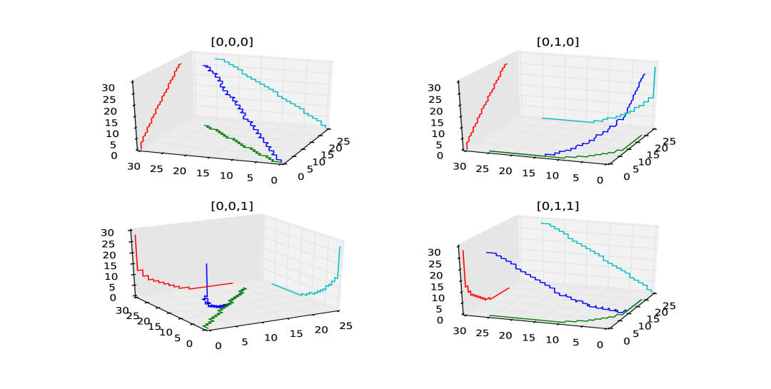
Figure 2: The blue curve in each graph is the support of an extreme measure in the case $J=3$, with Poisson marginal distributions. The red, teal, and green curves represent the projection of the 3D support onto the x-y, x-z, and y-z planes. These four graphs completely describe the support of the extreme measures in the case $J=3$.

The resulting extreme correlation matrices are as follows:

$${\mathbf{C}^{\vec{e}^{\,1}}}=\begin{pmatrix}1.0&0.93688&0.931861\\ 0.93688&1.0&0.967188\\ 0.931861&0.967188&1.0\\ \end{pmatrix}$$

$${\mathbf{C}^{\vec{e}^{\,2}}}=\begin{pmatrix}1.0&-0.81193&0.931861\\ -0.81193&1.0&-0.90135\\ 0.931861&-0.90135&1.0\\ \end{pmatrix}$$

$${\mathbf{C}^{\vec{e}^{\,3}}}=\begin{pmatrix}1.0&0.93688&-0.84624\\ 0.93688&1.0&-0.90135\\ -0.84624&-0.90135&1.0\\ \end{pmatrix}$$

$${\mathbf{C}^{\vec{e}^{\,4}}}=\begin{pmatrix}1.0&-0.81193&-0.84624\\ -0.81193&1.0&0.967188\\ -0.84624&0.967188&1.0\\ \end{pmatrix}$$

where $C^{\vec{e}^{\,i}}$ is the correlation matrix corresponding to the monotonicity structure defined by the vector $\vec{e}^{\,i},(i=1,2,3,4)$.

Extreme Measure 1		Extreme Measure 2
$(i_{1},i_{2},i_{3})$	$p^{\vec{e}^{\,1}}(i_{1},i_{2},i_{3})$	$(i_{1},i_{2},i_{3})$	$p^{\vec{e}^{\,2}}(i_{1},i_{2},i_{3})$
(0,0,0)	0.0009	(0,10,0)	0.0000
(0,0,1)	0.0058	(0,9,0)	0.0002
(0,1,1)	0.0006	(0,8,0)	0.0009
(0,1,2)	0.0223	(0,7,0)	0.0034
(0,1,3)	0.0108	(0,6,0)	0.0120
(0,2,3)	0.0094	(0,5,0)	0.0332
(1,2,3)	0.0320	(0,5,1)	0.0029
(1,2,4)	0.0429	(0,4,1)	0.0902
(1,3,4)	0.0483	(0,3,1)	0.0563
(1,3,5)	0.0262	(0,3,2)	0.1242
(2,3,5)	0.0659	(0,2,2)	0.0446
(2,4,5)	0.0357	(1,2,2)	0.0553
(2,4,6)	0.1225	(1,2,3)	0.1708
(3,4,6)	0.0173	(1,1,3)	0.0532
(3,5,6)	0.0092	(1,1,4)	0.0885
(3,5,7)	0.1490	(2,1,4)	0.0795
(3,5,8)	0.0172	(2,1,5)	0.0494
(3,6,8)	0.0313	(2,0,5)	0.0514
(4,6,8)	0.0819	(2,0,6)	0.0036
(4,6,9)	0.0331	(3,0,6)	0.0468
(4,7,9)	0.0531	(3,0,7)	0.0145
(5,7,9)	0.0152	(4,0,7)	0.0071
(5,7,10)	0.0361	(4,0,8)	0.0081
(5,8,10)	0.0349	(4,0,9)	0.0001
(5,8,11)	0.0146	(5,0,9)	0.0026
(6,8,11)	0.0158	(5,0,10)	0.0005
(6,9,11)	0.0147	(6,0,10)	0.0003
(6,9,12)	0.0198	(6,0,11)	0.0002
(7,9,12)	0.0017	(7,0,11)	0.0000
(7,10,12)	0.0048	(7,0,12)	0.0001

Table 1: Support and joint probabilities of the extreme measure corresponding to monotonicity structures $\vec{e}^{\,1}$ and $\vec{e}^{\,2}$

Extreme Measure 3		Extreme Measure 4
$(i_{1},i_{2},i_{3})$	$p^{\vec{e}^{\,3}}(i_{1},i_{2},i_{3})$	$(i_{1},i_{2},i_{3})$	$p^{\vec{e}^{\,4}}(i_{1},i_{2},i_{3})$
(0,0,13)	0.0000	(0,10,13)	0.0000
(0,0,12)	0.0001	(0,10,12)	0.0000
(0,0,11)	0.0002	(0,9,12)	0.0000
(0,0,10)	0.0008	(0,9,11)	0.0002
(0,0,9)	0.0027	(0,8,11)	0.0001
(0,0,8)	0.0081	(0,8,10)	0.0008
(0,0,7)	0.0216	(0,7,10)	0.0000
(0,0,6)	0.0504	(0,7,9)	0.0027
(0,0,5)	0.0514	(0,7,8)	0.0007
(0,1,5)	0.0494	(0,6,8)	0.0074
(0,1,4)	0.1680	(0,6,7)	0.0047
(0,1,3)	0.0151	(0,5,7)	0.0169
(1,1,3)	0.0381	(0,5,6)	0.0191
(1,2,3)	0.1708	(0,4,6)	0.0313
(1,2,2)	0.0999	(0,4,5)	0.0590
(1,3,2)	0.0591	(0,3,5)	0.0419
(2,3,2)	0.0651	(0,3,4)	0.1386
(2,3,1)	0.0563	(0,2,4)	0.0294
(2,4,1)	0.0626	(0,2,3)	0.0151
(3,4,1)	0.0276	(1,2,3)	0.2089
(3,5,1)	0.0029	(1,2,2)	0.0172
(3,5,0)	0.0308	(1,1,2)	0.1418
(4,5,0)	0.0024	(2,1,2)	0.0651
(4,6,0)	0.0120	(2,1,1)	0.0638
(4,7,0)	0.0009	(2,0,1)	0.0550
(5,7,0)	0.0026	(3,0,1)	0.0305
(5,8,0)	0.0005	(3,0,0)	0.0308
(6,8,0)	0.0004	(4,0,0)	0.0153
(6,9,0)	0.0002	(5,0,0)	0.0031
(7,9,0)	0.0000	(6,0,0)	0.0005

Table 2: Extreme measures corresponding to monotonicity structures $\vec{e}^{\,3}$ and $\vec{e}^{\,4}$

In Tables 1 & 2, we list the values of the joint probabilities $p^{\vec{e}}(\vec{i})$ for the extreme measures. Each table contains 2 of the 4 extreme measures. The columns are grouped such that they display the support and the corresponding joint probabilities corresponding to each example extreme measure.

5 Calibration of Correlations

In the case $J=2$, given a correlation coefficient $\rho$ in the admissible correlation range $[\rho^{*},\rho^{**}]$, we can use the following approach to find a probability measure $p$ having correlation $\rho$ and satisfying the marginal constraints. The approach is as follows. First find the unique $w\in[0,1]$ such that

$$\rho=w\rho^{*}+(1-w)\rho^{**}$$

Then set $p=w\,p^{*}+(1-w)\,p^{**}$, where $p^{*}$ and $p^{**}$ are the extreme measures with correlations $\rho^{*}$ and $\rho^{**}$, respectively. Note that $p$ has correlation $\rho$ and that it also satisfies the marginal constraints, as it is a convex combination of $p^{*}$ and $p^{**}$, both of which also satisfy the marginal constraints. Note also that, if $\rho$ is not in the admissible correlation range $[\rho^{*},\rho^{**}]$, then it cannot be the correlation of a probability measure $p$ satisfying the marginal constraints.

If $J>2$, the same idea is applicable. However, we have instead, a system of equations with $N_{w}$ weights to solve for a given correlation matrix

$$\mathcal{C}_{g}=w_{1}\,\mathcal{C}_{1}+\dots+w_{N_{w}}\,\mathcal{C}_{N_{w}},$$ (16)

where the $\mathcal{C}_{n}$ are correlation matrices associated with the extreme distributions, $w_{n}\geq 0$ and $\sum_{n=1}^{N_{w}}w_{n}=1$. Taking the extreme measures with the same set of marginal distributions, we construct the convex combination

$$p^{w}=w_{1}p^{e_{1}}\,+\dots+w_{N_{w}}p^{e_{N_{w}}}$$ (17)

where $p^{w}$ has correlation matrix $\mathcal{C}_{g}$ and satisfies the marginal constraints. The calibration problem is now reduced to finding a minimal $N_{w}$ to form a convex combination of extreme measures. Indeed, the number of extreme measures is $2^{J-1}$ and the number of correlation coefficients is $M=J(J-1)/2$. In matrix form (16) can be written as

$$Aw=\hat{\mathcal{C}}_{g}\\$$ (18)

where $A$ is of dimension $M$-by-$N$, the $i^{\mathrm{th}}$ column of $A$ is a vectorized version of the upper triangular part of the extreme correlation matrix $\mathcal{C}_{i}$ and $\hat{\mathcal{C}}_{g}$ is a vectorized version of the matrix $\mathcal{C}_{g}$. As the dimensionality of the multivariate Poisson process $J$ increases, $A$ becomes increasingly underdetermined. To find the weights, $w_{j}$, one can solve the following constrained system of equations

$$Aw=\hat{\mathcal{C}}_{g}$$ (19)

$$\textbf{1}^{T}w=1$$

$$w_{n}\geq 0\qquad n=1,2,\dots,N.$$

An approach to solving (19) is outlined on pages 376-379 of Nocedal and Wright, (2006). If (19) does not have a solution, this implies that the correlation matrix $\mathcal{C}_{g}$ cannot be generated from a multivariate Poisson process with the prescribed marginal distributions. Once we have found a $w$ satisfying the constraints (19), we can reduce the number of nonzero components in $w$ to $N_{w}\leq M+1$ using, for example a technique similar to that often used in the proof of Carathéodory’s theorem, to obtain a vector of $N_{w}$ nonzero weights satisfying (16) and the positivity constraints on $w$.

A matrix $\mathcal{C}$ is called admissible if it is a symmetric, positive semi-definite (PSD) matrix with ones on the diagonal and each entry satisfies $\rho_{ij}^{*}\leq c_{ij}\leq\rho_{ij}^{**}$, where $\rho_{ij}^{*}$ and $\rho_{ij}^{**}$ are extreme correlations for the $2$-dimensional problem for $(X_{i},X_{j})$. Notice that the correlation matrices corresponding to the extreme measures are admissible.

Theorem 5.1.

A convex combination of admissible correlation matrices is also an admissible correlation matrix.

Proof.

This fact readily follows from the observation that a convex combination of PSD matrices is a PSD matrix and, if all the matrices satisfy the correlation constraints so will the the convex combination of matrices. ∎

The probabilities $p^{\vec{e}}(\vec{i})$ describing the extreme measures and their supports are very different from the case of independent r.v.’s $X_{j}$. In particular, if $\rho=0$, the support of the measure $p^{w}$ is the union of the supports of $p^{\vec{e}}$. By adding an additional edge point $p^{0}$ corresponding to the case of independent components of $\vec{X}$, one can obtain a more general solution. We do not discuss this problem further in this paper.

Example Calibration

We continue with the example extreme measure (c.f. Section 4) and attempt to calibrate to a target correlation matrix, $C_{\ast}$, given by

$$C_{\ast}=\begin{pmatrix}1.0&-0.8&-0.5\\ -0.8&1.0&0.5\\ -0.5&0.5&1.0\\ \end{pmatrix}$$

Recall that in our example $J=3$, the Poisson marginal distributions have intensities $\boldsymbol{\mu}=(\mu_{1},\mu_{2},\mu_{3})=(3,5,7)$ and $N=2^{J-1}=4$ extreme points. In this case, the constrained system corresponding to can be constructed from the unique entries of the correlation matrix corresponding to each extreme point of the example extreme measure given in Section 4 and takes the following form:

$$\begin{pmatrix}0.93688&-0.81193&0.93688&-0.81193\\ 0.931861&0.931861&-0.84624&-0.84624\\ 0.967188&-0.90135&-0.90135&0.967188\\ 1&1&1&1\end{pmatrix}\begin{pmatrix}w_{1}\\ w_{2}\\ w_{3}\\ w_{4}\end{pmatrix}=\begin{pmatrix}-0.8\\ -0.5\\ 0.5\\ 1\end{pmatrix}$$

A unique solution to this is $w$ = (0.0287993, 0.205588, 0.0436342, 0.721979). Now let

$$p_{*}=w_{1}\cdot p^{\vec{e}^{1}}+w_{2}\cdot p^{\vec{e}^{2}}+w_{3}\cdot p^{\vec{e}^{3}}+w_{4}\cdot p^{\vec{e}^{4}}$$

where $p^{\vec{e}^{i}}$ is the extreme measure associate with the extreme correlation matrix $C^{\vec{e}^{i}}$, $i=1,2,3,4$, listed in Section 4. Note that $p_{*}$ has correlation matrix $C_{*}$ and $p_{*}$ also satisfies the marginal constraints, since each of $p^{\vec{e}^{i}}$, $i=1,2,3,4$, satisfies the marginal constraints.

6 Simulation

Up until this point, we have discussed the computation of the multivariate Poisson distribution at some terminal time $T$ via the EJD algorithm. That allows us to achieve extreme correlations between the components of the multivariate Poisson process at time $T$. We also obtain bounds on the elements of the admissible correlation matrix. The computation of the extreme measures allows us to construct any admissible multivariate Poisson process.

We briefly discuss the BS approach, which allows us to simulate the correlated multivariate Poisson processes on $[0,T]$ having an admissible correlation matrix at time $T$. Finally, we introduce the Forward continuation of the BS method. This extension allows us to construct sample paths of the multivariate Poisson process on the whole time axis.

Backward Simulation

There are two general approaches to simulation of the sample paths of multivariate Poisson processes—a Forward approach and a Backward approach. Under the Forward simulation approach, the Frechet-Hoeffding theorem can be used to generate the inter-arrival times of the components. The correlation boundaries for the components of the multivariate Poisson process are tighter than the correlation boundaries attained using the BS approach. Furthermore, the time structure of correlation is richer in the Backward case. See Kreinin, (2016) for a more detailed comparison.

The Backward approach relies on the conditional uniformity of the arrival times of the Poisson processes. More precisely, the conditional distribution of the (unordered) arrival moments, $T_{i}$, of a Poisson process in the interval $[0,T]$, conditional on the number of events in the interval is uniform Feigin, (1979).

The converse statement characterizing, the class of Poisson processes, is the foundation of the BS method Kreinin, (2016). Consider a process $N_{t},(t\geq 0)$ defined as

$$N_{t}=\sum^{N_{*}}_{i=1}\mathbbm{1}(T_{i}\leq t),\quad 0\leq t\leq T,$$

where $T_{i}$ are independent, identically distributed random variables uniformly distributed in the interval $[0,T]$. Notice that $N_{T}=N_{*}$.

Theorem 6.1.

Let $N_{*}$ have a Poisson distribution with parameter $\lambda T$. Then $N_{t}$ is a Poisson process with intensity $\lambda$ in the interval $[0,T]$.

Let us now formulate the generalization of Theorem 6.1. Suppose that coordinates of the random vector

$$N_{\ast}=\bigl{(}N^{(1)},\dots,N^{(J)}\bigr{)}$$

have Poisson distribution, $N^{(j)}_{\ast}\sim{\operatorname{Pois}}(\lambda_{j}T)$. Denote the correlation coefficient of $N^{(i)}_{\ast}$ and $N^{(j)}_{\ast}$ by $\rho_{ij}$.

Theorem 6.2.

Consider the processes

$$N^{(j)}_{t}=\sum_{i=1}^{N^{(j)}_{\ast}}{\mathbbm{1}}{\bigl{(}T_{i}^{(j)}\leq t\bigr{)}},\,\,j=1,2,\dots,J,$$

where the random variables, $T_{i}^{(j)},(i=1,2,\dots,N^{(j)}_{\ast})$, are mutually independent, uniformly distributed in the interval $[0,T]$. Then $\mathbf{N_{t}}=\bigl{(}N^{(1)}_{t},\dots,N^{(J)}_{t}\bigr{)}$ is a multivariate Poisson processes in the interval $[0,T]$ and

$$\text{corr}(N^{(i)}_{t},N^{(j)}_{t})=\rho_{ij}tT^{-1},\quad 0\leq t\leq T.$$ (20)

The proof can be found in Kreinin, (2016). Let us now formulate the BS method:

• Given a finite vector of weights, $w_{n}$, $(n=1,2,\dots,N_{w})$, satisfying the conditions $w_{n}\geq 0$, $\sum_{n=1}^{N_{w}}w_{n}=1$, generate an index, $n$ by sampling from the probability distribution defined by $w$ to choose an extreme measure, $p^{\vec{e_{n}}}$.

• Generate a random vector $\mathbf{N_{T}}=(N_{T}(1),\dots N_{T}(J))$ from the extreme measure $p^{\,e_{n}}$.

• Generate arrival moments of the multivariate process $\mathbf{N_{t}},(0\leq t\leq T)$. This can be accomplished via straightforward simulation of the uniform distribution and ordering in the ascending order of the resulting samples of the random variables $T_{j}$.

Forward Continuation of the Backward Simulation

The BS technique allows for the construction of sample paths of a multivariate Poisson process in an interval, $[0,T]$. In this section we consider an extension of the technique, which we call Forward-Backward simulation. We outline this approach for $J=2$.

Consider a sequence of time intervals $[0,T)$, $[T,2T)$, $\dots,[mT,(m+1)T]$. Suppose that a bivariate Poisson process, $(X_{t},Y_{t})$, has already been simulated in the interval $[0,T)$ using the BS technique. For any $\tau$, $0\leq\tau<T$, the increments $X_{T+\tau}-X_{T}$ are independent of $X_{T}$ and $Y_{T+\tau}-Y_{T}$ are independent of $Y_{T}$. Let us define the joint distribution of the increments as

$$(X_{T+\tau}-X_{T},Y_{T+\tau}-Y_{T}){\stackrel{{\scriptstyle{\cal D}}}{{=}}}(\hat{X}_{\tau},\hat{Y}_{\tau}),\quad 0<\tau\leq T,$$

where $\hat{X}_{\tau}$ and $\hat{Y}_{\tau}$ are independent versions of $X_{t}$ and $Y_{t}$, respectively, $\hat{X}_{\tau}{\stackrel{{\scriptstyle{\cal D}}}{{=}}}X_{t}$ and $\hat{Y}_{\tau}{\stackrel{{\scriptstyle{\cal D}}}{{=}}}Y_{t}$. Then we find

$$\operatorname{Cov}(X_{T+\tau},Y_{T+\tau})=\operatorname{Cov}(X_{T},Y_{T})+\operatorname{Cov}(X_{\tau},Y_{\tau}).$$

Taking into account that

$$\operatorname{Cov}(X_{\tau},Y_{\tau})=\operatorname{Cov}(X_{T},Y_{T})\cdot\frac{\tau^{2}}{T^{2}},$$

we obtain

$$\rho(T+\tau)=\rho(T)\frac{T^{2}+\tau^{2}}{T(T+\tau)}.$$

In particular, we have $\rho(2T)=\rho(T)$ and $\operatorname{Cov}(X_{2T},Y_{2T})=2\operatorname{Cov}(X_{T},Y_{T})$. Suppose now that $\rho(t)$ is defined for all $t\leq nT$.

Consider now the case $t=nT+\tau\in[nT,(n+1)T)$. We have

$$\operatorname{Cov}(X_{nT},Y_{nT})=n\operatorname{Cov}(X_{T},Y_{T})$$

and

$$\operatorname{Cov}(X_{nT+\tau},Y_{nT+\tau})=\operatorname{Cov}(X_{T},Y_{T})\cdot\Big{(}n+\frac{\tau^{2}}{T^{2}}\Big{)}.$$

This latter relation implies

$$\rho(nT+\tau)=\rho(T)\frac{n+\tau^{2}\cdot T^{-2}}{n+\tau T^{-1}},$$

and we obtain asymptotic stationarity of the correlation coefficient:

$$\lim_{n\to\infty}\rho(nT+\tau)=\rho(T)\quad\text{for all }\tau\in[0,T].$$

Thus, the processes $X_{t}$ and $Y_{t}$ exhibit asymptotically stationary correlations as $t\rightarrow\infty$. An illustration of this is shown in Figure 3, where maximal (red line) and minimal (blue line) values of the correlation coefficient, $\text{corr}(X_{t},Y_{t})$ are depicted.

It would be interesting to generalize this result for the class of mixed Poisson processes. The main difficulty is that the increments of the mixed Poisson processes are not independent.

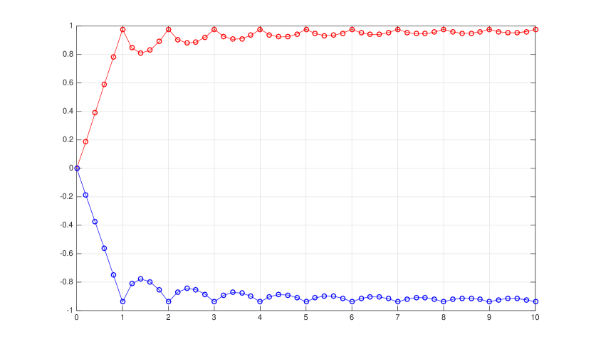
Figure 3: Forward Continuation of Backward Simulation: $\text{corr}(X_{t},Y_{t})$, $\mu_{1}=3$, $\mu_{2}=5$.

7 Final remarks

We presented an approach to the solution to the problem of simulation of multivariate Poisson processes in the case the dimension of the problem is $J>2$ and we described the admissible parameters for the calibration problem. We also extended the BS approach with the introduction of the Forward Continuation of BS.

There are several directions for future research. One is to extend the EJD approach to more general processes such as the Mixed Poisson processes and even to multivariate jump-diffusion processes. Another avenue of future research may be concerned with the efficient solutions of the multivariate calibration problem.

It would also be interesting to study the interplay between the optimization problem and the EJD algorithm for computing the probabilities of the extreme measures and find the interpretation of this algorithm in terms of the Optimal transport problem. Exploring the synthesis of Forward and Backward simulation for more general processes is also worthwhile.

References

- Aue and Kalkbrener, (2006) Aue, F. and Kalkbrener, M. (2006). LDA at work: Deutsche bank’s approach to quantifying operational risk. Journal of Operational Risk, 1(4):49–93.
- Bae and Kreinin, (2017) Bae, T. and Kreinin, A. (2017). A backward construction and simulation of correlated poisson processes. Journal of Statistical Computation and Simulation, 87(8):1593–1607.
- Böcker and Klüppelberg, (2010) Böcker, K. and Klüppelberg, C. (2010). Multivariate models for operational risk. Quantitative Finance, 10(8):855–869.
- Chavez-Demoulin et al., (2006) Chavez-Demoulin, V., Embrechts, P., and Nešlehová, J. (2006). Quantitative models for operational risk: extremes, dependence and aggregation. Journal of Banking & Finance, 30(10):2635–2658.
- Duch et al., (2014) Duch, K., Jiang, Y., and Kreinin, A. (2014). New approaches to operational risk modeling. IBM Journal of Research and Development, 58(4):3–1.
- Embrechts and Puccetti, (2006) Embrechts, P. and Puccetti, G. (2006). Aggregating risk capital, with an application to operational risk. The Geneva Risk and Insurance Review, 31(2):71–90.
- Feigin, (1979) Feigin, P. D. (1979). On the characterization of point processes with the order statistic property. Journal of Applied Probability, 16(2):297–304.
- Fréchet, (1960) Fréchet, M. (1960). Sur les tableaux dont les marges et des bornes sont données. Revue de l’Institut international de statistique, pages 10–32.
- Kreinin, (2016) Kreinin, A. (2016). Correlated poisson processes and their applications in financial modeling. Financial Signal Processing and Machine Learning, pages 191–232.
- Lindskog and McNeil, (2001) Lindskog, F. and McNeil, A. (2001). Poisson shock models: applications to insurance and credit risk modeling. Federal Institute of Technology ETH Zentrum, Zurich, pages 1280–1289.
- Nocedal and Wright, (2006) Nocedal, J. and Wright, S. J. (2006). Numerical Optimization. Springer.
- Panjer, (2006) Panjer, H. H. (2006). Operational risk: modeling analytics, volume 620. John Wiley & Sons.
- Powojowski et al., (2002) Powojowski, M. R., Reynolds, D., and Tuenter, H. J. (2002). Dependent events and operational risk. Algo Research Quarterly, 5(2):65–73.
- (14) Rachev, S. T. and Rüschendorf, L. (1998a). Mass Transportation Problems: Volume I: Theory, volume 1. Springer Science & Business Media.
- (15) Rachev, S. T. and Rüschendorf, L. (1998b). Mass Transportation Problems: Volume II: Applications, volume 2. Springer Science & Business Media.
- Shevchenko, (2011) Shevchenko, P. V. (2011). Modelling operational risk using Bayesian inference. Springer Science & Business Media.
- Villani, (2008) Villani, C. (2008). Optimal transport: old and new, volume 338. Springer Science & Business Media.