Spatial Models with the Integrated Nested Laplace Approximation within Markov Chain Monte Carlo

Abstract

The Integrated Nested Laplace Approximation (INLA) is a convenient way to obtain approximations to the posterior marginals for parameters in Bayesian hierarchical models when the latent effects can be expressed as a Gaussian Markov Random Field (GMRF). In addition, its implementation in the R-INLA package for the R statistical software provides an easy way to fit models using INLA in practice. R-INLA implements a number of widely used latent models, including several spatial models. In addition, R-INLA can fit models in a fraction of the time than other computer intensive methods (e.g. Markov Chain Monte Carlo) take to fit the same model.

Although INLA provides a fast approximation to the marginals of the model parameters, it is difficult to use it with models not implemented in R-INLA. It is also difficult to make multivariate posterior inference on the parameters of the model as INLA focuses on the posterior marginals and not the joint posterior distribution.

In this paper we describe how to use INLA within the Metropolis-Hastings algorithm to fit spatial models and estimate the joint posterior distribution of a reduced number of parameters. We will illustrate the benefits of this new method with two examples on spatial econometrics and disease mapping where complex spatial models with several spatial structures need to be fitted.

1 Introduction

Bayesian inference on complex hierarchical models have relied on Markov Chain Monte Carlo (MCMC, henceforth) methods for many years. Inference with MCMC is based on drawing samples from the joint posterior distribution of the model parameter, and this is often of a high dimension. For Bayesian hierarchical models with complex structure or large datasets, MCMC can be very computationally demanding. See, for example, Gilks et al. [11] and Brooks et al. [8] for a summary of MCMC methods.

To avoid dealing with high dimensional posterior distributions that are hard to estimate, Rue et al. [31] focus on marginal inference and they develop a method to approximate the posterior marginal of the model parameters using the Laplace approximation and numerical integration. Also, they focus on models whose latent effects are a Gaussian Markov Random Field (GMRF, henceforth). GMRFs have several properties that can be exploited for computational efficiency when fitting Bayesian models [30]. This new method has been termed the Integrated Nested Laplace Approximation (INLA, henceforth) and an implementation is available in the R-INLA package, that can cope with a large family of models.

Bivand et al. [4] describe a novel approach to fit models not implemented in R-INLA with INLA. They note that some models can be fitted with R-INLA when one of the parameters is fixed, such as several models widely used in spatial econometrics [21]. In this particular case, the models can be fitted when the spatial autocorrelation parameter is fixed. As this parameters is in a bounded interval, values for the spatial autocorrelation parameters can be taken from a fine grid on its (bounded) support. Conditioning on these values, models can be fitted to obtain conditional posterior marginals of all the other parameters. The posterior marginal of the spatial autocorrelation parameter is then obtained by combining the marginal likelihoods of the fitted models and the prior using Bayes’ rule. The posterior marginals for the remainder of the parameters in the model is obtained by averaging over the different conditional posterior marginals.

The former method can be easily extended to more than one parameter but as the number of parameter increases the number of models to be fitted increases exponentially. Also, it is problematic when the parameters that need to be fixed are not in a bounded interval. Hence, if the model needs to be conditioned on several parameters to be fitted with R-INLA, a different approach is required.

Gómez-Rubio and Rue [15] suggest using the Metropolis-Hastings algorithm [27, 18] together with INLA when models need to be conditioned on several parameters. In this way, the joint posterior distribution of an ensemble of parameters can be obtained via MCMC, whilst the posterior marginals of all the other parameters is obtained by averaging over several conditional marginal distributions.

In this paper we extend the work presented in Gómez-Rubio and Rue [15] by considering specific applications to spatial statistics. In particular, we consider complex spatial econometrics models and models for disease mapping with several spatial components.

This paper is structured as follows. Section 2 provides a summary of INLA and the R-INLA package. A detailed description of the spatial models implemented in R-INLA is given in Section 3. Next, Section 4 covers how INLA can be used within the Metropolis-Hastings algorithm to fit new spatial models. This is illustrated in Section 5, where two examples on spatial econometrics and joint disease mapping are developed. Finally, a summary and discussion is available in Section 6.

2 Integrated Nested Laplace Approximation

In this Section we will outline the main details about INLA, which is fully described in Rue et al. [31]. Let us assume that we have a vector $\bm{y}=(y_{1},\ldots,y_{n})$ of $n$ observations with a likelihood from the exponential family. Mean $\mu_{i}$ is assumed to be linked, using an appropriate function, to a linear predictor $\eta_{i}$ that will depend on some latent effects $\bm{x}$. This is often expressed as

$$\eta_{i}=\alpha+\sum_{j=1}^{n_{\beta}}\beta_{j}z_{ji}+\sum_{k=1}^{n_{f}}f^{(j)}(u_{ki})+\varepsilon_{i}$$ (1)

In this equation, $\alpha$ is an intercept, $\beta_{j}$ are $n_{\beta}$ coefficients on some covariates $\bm{z}$, $f^{(k)}$ represent functions on $n_{f}$ random effects on a vector of covariates $\bm{u}$, and $\varepsilon_{i}$ is an error term. Hence, the vector of latent effects can be written as

$$\bm{x}=\left(\eta_{1},\ldots,\eta_{n},\alpha,\beta_{1},\ldots\right)$$ (2)

Rue et al. [31] assume that the structure of the latent effects $\bm{x}$ is a Gaussian Markov Random Field [see, 30, for a detailed description]. The precision matrix $\bm{Q}(\theta_{1})$ will depend on a number of hyperparameters $\theta_{1}$ and it will fulfill a number of Markov properties to define the dependences between the elements in the latent effects. For this reason, $\bm{Q}(\theta_{1})$ is often very sparse.

Also, observations in $\bm{y}$ are independent given the values of the latent effects $\bm{x}$ and their distribution may depend on a number of hyperparameters $\theta_{2}$.

This means that the posterior distribution of the latent effects $\bm{x}$ and the vector of hyperparameters $\theta=(\theta_{1},\theta_{2})$ can be written down as:

$$\pi(\bm{x},\theta|\bm{y})=\frac{\pi(\bm{y}|\bm{x},\theta)\pi(\bm{x},\theta)}{\pi(\bm{y})}\propto\pi(\bm{y}|\bm{x},\theta)\pi(\bm{x},\theta)$$ (3)

$\pi(\bm{y})$ is the marginal likelihood and it is a normalizing constant that is usually ignored because it is often difficult to compute. Nevertheless, R-INLA provides an accurate approximation to this quantity that will play an important role, as we will see later.

In addition, $\pi(\bm{y}|\bm{x},\theta)$ is the likelihood of the model. As we are assuming that observations $(y_{1},\ldots,y_{n})$ are independent given $\bm{x}$ and $\theta$, then

$$\pi(\bm{y}|\bm{x},\theta)=\prod_{i\in\mathit{I}}\pi(y_{i}|\bm{x},\theta)$$ (4)

$\mathit{I}$ is a set of indices from 1 to $n$ that represents the actually observed values of $y_{i}$, i.e., if $y_{j}$ is missing then $j$ is not in $\mathit{I}$.

Joint distribution $\pi(\bm{x},\theta)$ can be expressed as $\pi(\bm{x}|\theta)\pi(\theta)$. Given that $\bm{x}$ is a GMRF, we have the following:

$$\pi(\bm{x}|\theta)\propto|\bm{Q}(\theta)|^{1/2}\exp\{-\frac{1}{2}\bm{x}^{T}\bm{Q}(\theta)\bm{x}\}$$ (5)

Finally, $\pi(\theta)$ is the prior distribution of the ensemble of hyperparameters $\theta$. Provided that most of them are independent a priori, $\pi(\theta)$ can be decomposed as the product of several (univariate) distributions.

Hence, the joint posterior distributions of the latent effects and parameters can be written down as

$$\pi(\bm{x},\theta|\bm{y})\propto\pi(\theta)|\bm{Q}(\theta)|^{1/2}\exp\{-\frac{1}{2}\bm{x}^{T}\bm{Q}(\theta)\bm{x}\}\prod_{i\in\mathit{I}}\pi(y_{i}|\bm{x},\theta)=$$

$$\pi(\theta)|\bm{Q}(\theta)|^{1/2}\exp\{-\frac{1}{2}\bm{x}^{T}\bm{Q}(\theta)\bm{x}+\sum_{i\in\mathit{I}}\log(\pi(y_{i}|\bm{x},\theta))\}$$ (6)

It should be noted that because $\bm{x}$ is a GMRF its precision matrix $\bm{Q}(\theta)$ is likely to be very sparse and this can be exploited for computational purposes.

The posterior marginal distributions of the latent effects can be written as

$$\pi(\bm{x}_{i}|\bm{y})=\int\pi(\bm{x}_{i},\theta|\bm{y})\pi(\theta|\bm{y})d\theta$$ (7)

Similarly, the posterior marginal of hyperparameter $\theta_{i}$ can be written as

$$\pi(\theta_{i}|\bm{y})=\int\pi(\theta|\bm{y})d\theta_{-i}$$ (8)

where $\theta_{-i}$ is the vector of parameters $\theta$ excluding $\theta_{i}$.

Rue et al. [31] propose an approximation to the joint posterior of $\theta$, $\tilde{\pi}(\theta|\bm{y})$, that can be used to compute the marginals of latent effects and parameters:

$$\tilde{\pi}(\theta|\bm{y})\propto\frac{\pi(\bm{x},\theta,\bm{y})}{\tilde{\pi}_{G}(\bm{x}|\theta,\bm{y})}\Big{|}_{\bm{x}=\bm{x}^{*}(\theta)}$$ (9)

Here, $\tilde{\pi}_{G}(\bm{x}|\theta,\bm{y})$ is an approximation to the full conditional of $\bm{x}$ using a Gaussian distribution, and $\bm{x}^{*}(\theta)$ is the mode of the full conditional for a given $\theta$.

Approximation $\tilde{\pi}(\theta|\bm{y})$ can be used to compute $\pi(\theta_{i}|\bm{y})$ (by integrating $\theta_{-i}$ out) and $\pi(x_{i}|\bm{y})$, using numerical integration on equation (7), but this also requires a good approximation to $\pi(x_{i},\theta|\bm{y})$. A Gaussian approximation can be used as well, but Rue et al. [31] develop better approximations using other methods such as the Laplace approximation.

More details can be found in Blangiardo and Cameletti [6] (Chapter 4), where computational details are clearly explained and a full example for a Normal-Gamma model is developed.

INLA is implemented as an R [29] package named R-INLA. In addition to providing a simple way of defining models and computing the approximation to the posterior marginals, R-INLA provides some extra features for model specification[see, 26, for details] and can compute a number of derived quantities for model checking and model assessment . In particular, an approximation to the marginal likelihood of the model $\pi(\bm{y})$ is provided, which can also be used for model selection, for example.

3 Spatial Models in INLA

Several authors [12, 5, 23, 6] summarize the different spatial models available in R-INLA as latent effects that can be used to build models. We will provide a summary in this Section in order to provide an overview of what has already been implemented and what other spatial models have not been added yet.

Spatial latent effects for lattice data in R-INLA have a prior distribution which is a multivariate Normal distribution with zero mean and precision matrix $\tau T$, where $\tau$ is a precision parameter and $T$ is a square and symmetric matrix. The structure of $T$ will control how the spatial dependence is and it can take different forms to induce different types of spatial interaction.

For a completely specified $T$, the multivariate Normal with zero mean and generic precision matrix $\tau T$ is implemented as the generic0 latent effect. This can be used to define flexible spatial structures in case they are not implemented, but matrix $T$ must be fully defined and it cannot depend on further parameters.

Besag et al. [2] proposed the use of an intrinsic CAR specification as a prior for spatial effects that is widely used nowadays. This is implemented in model besag and corresponds to the precision matrix $\tau Q$, with $Q$ defined as

$$Q_{ij}=\left\{\begin{array}[]{cc}n_{i}&i=j\\ -1&i\sim j\\ 0&\textrm{otherwise}\end{array}\right.1\leq i,j\leq n$$ (10)

Here, $n_{i}$ is the number of neighbors of region $i$, and $i\sim j$ indicates that regions $i$ and $j$ are neighbors. In this case, spatial random effects have the additional constrain to sum up to zero in order to make the model identifiable.

Similarly, the generic1 model implements a multivariate Normal with zero mean and precision matrix $\tau T$, with

$$T=(I-\frac{\beta}{\lambda_{max}}C)$$ (11)

Here, $\beta$ is a parameter which can take values between 0 and 1 and $\lambda_{max}$ is the maximum eigenvalue of matrix $C$. This latent effect can be used to implement the model proposed in Leroux et al. [20]. They propose a model in which the precision matrix is a convex combination of a diagonal matrix $I$ and matrix $Q$, i.e., the precision matrix is $(1-\lambda)I+\lambda Q$ with $\lambda\in(0,1)$. Ugarte et al. [34] show that when $C=I-Q$ then $\lambda_{max}=1$. Hence, the model by Leroux et al. [20] can be implemented in R-INLA with a generic1 model by taking $C=I-Q$, so that $T=I-\beta(I-Q)=(1-\beta)I+\beta Q$ with $\beta\in(0,1)$.

In addition to the intrinsic CAR specification implemented in model besag, model bym implements the sum of an intrinsic CAR and independent random effects described in Besag et al. [2]. Latent model properbesag implements a proper version of the intrinsic CAR specification by using a non-singular precision matrix with structure defined as

$$Q^{\prime}_{ij}=\left\{\begin{array}[]{cc}n_{i}+d&i=j\\ -1&i\sim j\\ 0&\textrm{otherwise}\end{array}\right.1\leq i,j\leq n$$ (12)

Here $d>0$ is an extra parameter that is added to the entries in the diagonal to make the precision matrix non-singular. Note that this precision matrix structure $Q^{\prime}$ is the same as in the besag model with an added $d$ to all the elements in the diagonal so that the resulting distribution is proper, i.e., $Q^{\prime}=Q+dI$.

Other models that can be used for spatial modeling are the two dimensional random walk (named rw2d) and a Gaussian field defined in a regular lattice with Matérn correlation function (model matern2d).

All the previous latent models were defined in a lattice, but the spde model [24] can be used to define a continuous process with a Matérn covariance. This means that it can be used for models in geostatistics and point patterns [32, 14].

Blangiardo et al. [7] and Blangiardo and Cameletti [6] describe how to combine these latent effects for spatio-temporal modeling. In addition, Bivand et al. [5] describe how to use the INLABMA package [5] to fit other spatial models using the ideas in Bivand et al. [4]. In particular, they fit the model proposed by Leroux et al. [20] and the spatial lag model [1, 21], commonly used in spatial econometrics. A new latent effect named slm [13] is available (but still experimental) to fit spatial econometrics models.

4 INLA within Markov Chain Monte Carlo

As described in the previous Section, R-INLA provides a large number of spatial latent effects that can be used to build more complex models. However, this is list is far from exhaustive and it is difficult to implement new models in R-INLA. A possible approach to implement new models is the rgeneric latent effect that allows the user to define the latent model in R but this requires the user to specify the full structure of the latent effect as a GMRF.

In order to extend the number of models that INLA can fit through the R-INLA package, Gómez-Rubio and Rue [15] propose the use of the Metropolis-Hastings algorithm [27, 18] together with INLA to fit some complex models not implemented in R-INLA.

Let us denote by $\theta$ the ensemble of parameters and hyperparameters to be estimated in a Bayesian hierarchical models. Note that now $\theta$ will include some of the latent effects in $\bm{x}$ and not only the hyperparameters $\theta_{1}$ and $\theta_{2}$ described in Section 2. Similarly as Bivand et al. [4], Gómez-Rubio and Rue [15] argue that very complex spatial models can be fitted with R-INLA when some of the parameters are fixed. Let us call these parameters $\theta_{c}$ so that $\theta$ becomes $(\theta_{c},\theta_{-c})$. By conditioning on $\theta_{c}$, INLA can be used to obtain the posterior marginals of all the parameters in $\theta_{-c}$, i.e., $\pi(\theta_{-c,i}|\bm{y},\theta_{c})$, and the conditional marginal likelihood $\pi(\bm{y}|\theta_{c})$.

Li et al. [22] deal with complex spatio-temporal models in a similar way by conditioning on some of the parameters at their maximum likelihood estimates. Although this is a reasonable way to proceed for highly parameterized models, it ignores the uncertainty of some of the parameters in the model when computing the posterior marginal of the other model parameters. Bivand et al. [4] also fit spatial models conditioning on some of the model parameters at different values in a grid and then combine the resulting models to obtain the posterior marginals (not conditioned on $\theta_{c}$) for the model of interest.

The Metropolis-Hastings algorithm could be used to draw values for $\theta_{c}$ so that its joint posterior distribution can be obtained. At step $i+1$ of the Metropolis-Hastings algorithm, new values $\theta_{c}^{(i+1)}$ for $\theta_{c}$ are proposed, but not necessarily accepted, from a proposal distribution $q(\theta_{c}^{(i+1)}|\theta_{c}^{(i)})$. The new values are accepted with probability

$$\alpha=\min\{1,\frac{\pi(\bm{y}|\theta_{c}^{(i+1)})\pi(\theta_{c}^{(i+1)})q(\theta_{c}^{(i)}|\theta_{c}^{(i+1)})}{\pi(\bm{y}|\theta_{c}^{(i)})\pi(\theta_{c}^{(i)})q(\theta_{c}^{(i+1)}|\theta_{c}^{(i)})}\}$$ (13)

If the proposed value is not accepted, then $\theta_{c}^{(i+1))}$ is set to $\theta_{c}^{(i))}$.

Note that $\pi(\bm{y}|\theta_{c}^{(i+1)})$ is the marginal likelihood of the model conditioned on $\theta_{c}^{(i+1)}$, which can be obtained by fitting the model by fixing the values of $\theta_{c}$ to $\theta_{c}^{(i+1)}$. Also, this will provide the posterior marginals $\pi(\theta_{-c,i}|\bm{y},\theta_{c}^{(i+1)})$ for all the parameters in $\theta_{-c}$.

After a suitable number of iterations, the Metropolis-Hastings algorithm will produce samples from $\pi(\theta_{c}|\bm{y})$, from which the the posterior marginals of the parameters in $\theta_{c}$ can be derived. Also, we will obtain a family of conditional marginal distributions for all the parameters in $\theta_{-c}$. Their posterior marginals can be obtained by combining all these marginals as follows:

$$\pi(\theta_{-c,i}|\bm{y})=\int\pi(\theta_{c,i}|\bm{y},\theta_{c})\pi(\theta_{c}|\bm{y})d\theta_{c}\simeq\frac{1}{N}\sum_{j=1}^{N}\pi(\theta_{c,i}|\bm{y},\theta_{c}^{(j)})$$ (14)

Values $\{\theta_{c}^{(j)}\}_{j=1}^{N}$ represent $N$ samples from $\pi(\theta_{c}|\bm{y})$ obtained with the Metropolis-Hastings algorithm.

Gómez-Rubio and Rue [15] illustrate the use of INLA within the Metropolis-Hastings algorithm with three examples, including fitting a simple spatial econometrics model. In addition to fitting models with unimplemented latent effects, this approach can be employed to use other priors not implemented in R-INLA (in particular, multivariate priors) and to fit models with missing values in the covariates. Cameletti et al. [9] discuss how models with missing data and multiple imputation can be tackled with INLA.

5 Examples

In this Section we provide two examples on how to fit complex spatial models with INLA using the R-INLA package and the Metropolis-Hastings algorithm. Both models have a complex spatial structure, with several spatial terms, and they cannot be fitted with R-INLA alone. In addition, to fitting the model, we show how to exploit the joint posterior distribution obtained on a reduced ensemble of parameters to make multivariate inference.

5.1 Spatial Econometrics

Manski [25] proposed the following general model for spatial econometrics that accounts for different levels of spatial dependence and interaction:

$$y=\rho Wy+X\beta+WX\gamma+u;\ u=\lambda Wu+e$$ (15)

$y$ is the response variable made of observations in $n$ areas, $W$ an adjacency matrix, $X$ a matrix of $p$ covariates, $WX$ a matrix of lagged covariates, $\beta$ and $\gamma$ associated coefficients, and $\rho$ and $\lambda$ are spatial autocorrelation parameters. $e$ is a multivariate Gaussian error term with zero mean and diagonal variance-covariance matrix $\sigma^{2}I$, where $I$ is the identity matrix of appropriate dimension.

This model has two autocorrelation terms, one on the response $y$ and another one on the error term $u$, that are controlled by autocorrelation parameters $\rho$ and $\lambda$, respectively. Spatial adjacency matrix $W$ is often taken as a binary matrix, so that entry at row $i$ and column $j$ will be 1 if areas $i$ and $j$ are neighbors. Although this is a reasonable adjacency matrix, we will take $W$ to be row-standardized, so that the sum of all the elements in a row add up to 1. This will bring interesting properties to the spatial autocorrelation parameters. In particular, they will be bounded in the interval $(1/\lambda_{min},1)$, where $\lambda_{min}$ is the minimum eigenvalue of $W$ [17].

LeSage and Pace [21] fit this model using Bayesian inference, for which they assign priors to all model parameters. In particular, they consider typical independent inverted gamma priors for all the precisions, vague independent Normal distributions for $\beta$ and $\gamma$ and uniform prior distribution for $\rho$ and $\lambda$ in the interval $(1/\lambda_{min},1)$.

In order to assess whether Manki’s model can be fitted using standard software for linear regression, it can be rewritten as follows:

$$y=(I-\rho W)^{-1}(X\beta+WX\gamma)+u;u\sim MVN(0,\Sigma)$$ (16)

Here, the error term has a multivariate normal distribution with zero mean and variance-covariance matrix $\Sigma=\sigma^{2}[(I-\rho W^{\prime})(I-\lambda W^{\prime})(I-\lambda W)(I-\rho W)]^{-1}$.

Hence, this model has a non-linear term on $\rho$, $(I-\rho W)^{-1}$, that multiplies the linear predictor on the covariates and lagged covariates, and a complex error structure. This model cannot be fitted with R-INLA unless we condition on $\rho$ and $\lambda$.

In order to fit this model with R-INLA, we have combined INLA and MCMC as described in this paper. In particular, we will be drawing samples from the posterior of $\theta_{c}=(\rho,\lambda)$ using the Metropolis-Hastings algorithm. At each step of the algorithm we will obtain a conditional (on $\theta_{c}$) posterior marginal for the remainder of the parameters in the model $\theta_{-c}$. These conditional marginals will be later combined to obtain the posterior marginals of the model parameters $\theta_{-c}$.

The proposal distribution for $\theta_{c}$ has been the product of two Normal distribution centered at the current value of the parameters and standard deviation 0.25. This value has been obtained after some tuning to ensure a suitable acceptance rate. The starting point is $\theta_{c}=(0,0)$. Then 500 iterations were used as burn-in, followed by 5000 iterations more, of which one in 5 was kept to reduce autocorrelation. This provided a final 1000 samples to estimate the joint posterior distribution of $\theta_{c}$. Note that thinning also involves the conditional distributions computed at each step of the Metropolis-Hastings algorithm.

We have fit this model to the Columbus dataset [1] which is available in R package spdep. This dataset contains information about 49 neighborhoods in Columbus (Ohio) in 1980. We will reproduce a classical analysis consisting on explaining crime rate on housing value (variable HOVAL) and household income (variable INC). We have not include lagged covariates, so that $\gamma=0$.

In addition to using INLA within MCMC as described in this paper, we have also fitted this model using Gibbs sampling using the rjags package [28] and using maximum likelihood with function sacsarlm() from the spdep package [3].

Figure 1 shows the posterior marginals distributions of the autocorrelation parameters, estimated using MCMC and INLA within MCMC, and the maximum likelihood estimates of the parameters. As it can be seen, there is good agreement between the different estimates. Regarding the other parameters in the model, Figure 2 summarizes the different estimates and how they seem to agree. Note that these marginals have been obtained by averaging the conditional marginals obtained at each step of the Metropolis-Hastings algorithm.

Figure 1: Estimates of the spatial autocorrelation parameters of the Manski model using INLA within MCMC, MCMC and maximum likelihood.

Figure 2: Estimates of the intercept, covariate coefficients and variance using INLA within MCMC, MCMC and maximum likelihood. Covariates are housing value (HOVAL) and household income (INC).

Finally, the joint posterior distribution of $(\rho,\lambda)$ is shown in Figure 3. The bivariate distributions obtained with INLA within MCMC and MCMC look alike. The maximum likelihood estimate has also been added to the plots (as a black dot), and in both plots looks close to the mode of the joint posterior distribution.

Figure 3: Joint posterior distribution of $(\rho,\lambda)$. The solid dot represents the maximum likelihood estimate.

5.1.1 Computation of the impacts

Spill over effects, or how changes in the covariates in one area affect its neighbors, are of interest in spatial econometrics. These measures are often called impacts and they are defined using partial derivatives as

$$\frac{\partial y_{i}}{\partial x_{jr}}\ i,j=1\ldots,n;\ r=1,\ldots,p$$ (17)

Each covariate will have an associated matrix of impacts which, for the model that we are considering, is:

$$S_{r}(W)=[I-\rho W]^{-1}(\beta_{r}+W\gamma_{r}),\ r=1,\ldots,p$$ (18)

Note that each element in that matrix will measure how a change in covariate $r$ in area $j$ will impact on the response in area $i$. These are often summarized as the average direct, indirect and total impacts.

Direct impacts measure changes in the response in the same area where the change occurs, indirect impacts measure changes in adjacent areas and total impacts are the sum of direct and indirect impacts. For this reason the average direct impact is defined as the mean of the trace of the impacts matrix, the average indirect impact is the sum of all the off-diagonal impacts divided by $n$ and the total impact is the sum of all the elements in the impacts matrix divided by $n$.

Following the details in LeSage and Pace [21] and Gómez-Rubio et al. [16], the average total impact for the Manski model for a covariate $r$ is

$$\frac{1}{1-\rho}\beta_{r},$$ (19)

and the average direct impact is

$$n^{-1}tr((I-\rho W)^{-1})\beta_{r}+n^{-1}tr((I-\rho W)^{-1}W)\gamma_{r}.$$ (20)

Here, $tr(\cdot)$ denotes the trace of a matrix. Average indirect impacts can be obtained by taking the difference between total and direct impacts.

As discussed in Gómez-Rubio et al. [16], computing the impacts requires multivariate inference as the distribution depends on the (joint) posterior distribution of $\rho$, $\beta_{r}$ and $\gamma_{r}$. Hence, computing the impacts from the posterior marginals of these parameters alone is not enough to obtain accurate estimates. Note that in our particular case we are not considering lagged covariates and that $\gamma_{r}=0$, which simplifies the computation of the impacts.

To compute the impacts we can exploit the fact that we have different models conditioned on the values of $\rho$. Hence, we could compute the marginal distribution of the impacts for each value of $\rho$ obtained with the Metropolis-Hastings and conditional (on $\rho$) marginal $\pi(\beta_{r}|y,\rho)$. Then we could average over all the conditional marginal distributions of the impacts given $rho$ to obtain the final distribution of the impacts, which could be used to compute summary statistics.

Table 1 summarizes the point estimates and standard deviations of the different average impacts considered in this example. The estimation methods for which the impacts are reported are MCMC, INLA within MCMC and maximum likelihood. MCMC and INLA within MCMC provided very similar results, although the latter seems to provide estimates with slightly smaller standard deviations.

	INC			HOVAL
Method	Direct	Indirect	Total	Direct	Indirect	Total
MCMC	-0.96 (0.37)	-0.46 (0.42)	-1.42 (0.66)	-0.30 (0.10)	-0.14 (0.14)	- 0.44 (0.20)
INLA+MCMC	-0.97 (0.33)	-0.44 (0.35)	-1.40 (0.48)	-0.30 (0.10)	-0.13 (0.10)	-0.43 (0.14)
Max. lik.	-1.10	-0.55	-1.65	-0.29	-0.15	-0.44

Table 1: Mean and standard deviation (in parenthesis) of the impacts for the Manski model without lagged covariates fitted to the Columbus dataset. Covariates are housing value (HOVAL) and household income (INC).

5.2 Joint Modeling of Three Diseases

Spatial models have been used for a long time in disease mapping to study the spatial variation of disease [6]. Several authors have used INLA to fit spatial and spatio-temporal models for disease mapping of a single disease as MCMC methods are often very slow when the number of areas is large. Modeling several diseases is more complex and it often involves non-linear terms on some parameters in the linear predictor of the model [20, 5]. Knorr-Held and Best [19] have considered the joint modeling of two diseases by including a shared spatial effect (with different weights for each disease) plus specific spatial terms for each disease.

In the next example we extend this model to three diseases following Downing et al. [10]. They fit a joint model to six diseases with different weighted shared and specific spatial components. In our case, we will only consider three diseases, which are modeled using a shared spatial term and specific spatial patterns.

In particular, let us assume that we have a study region divided into $n$ smaller areas and that we are interested in modeling $D$ diseases. Observed counts of disease $d$ in area $i$ will be denoted by $O^{(d)}_{i}$. Similarly, $E^{(d)}_{i}$ will represent the expected cases of disease $d$ in area $i$. The model that we will be fitting is

$$O^{(d)}_{i}\sim Po(E^{(d)}_{i}\theta^{(d)}_{i})$$ (21)

Here, $\theta^{(d)}_{i}$ is the relative risk for disease $d$ in area $i$, which is modeled as

$$\log(\theta^{(d)}_{i})=\alpha^{(d)}+v_{i}\cdot\delta^{(d)}+s^{(d)}_{i};\ i=1,\ldots,n;\ d=1,\ldots,D$$ (22)

Parameter $\alpha^{(d)}$ is a disease-specific intercept and it sets the baseline of the log-relative risks for disease $d$, $v_{i}$ is a shared component to all diseases, $\delta^{(d)}$ is a parameter that controls how the shared component affects disease $d$ and $s^{(d)}_{i}$ are specific components to each disease. The shared and specific components can include different types of fixed and random effects. Knorr-Held and Best [19] use a partition model to split areas into regions of similar risk, but other effects can be considered [see, for example, 33].

Note that this model looks like a standard log-linear model and that, for a fixed value of $\delta^{(d)}$, it could be fitted with some standard software packages for Bayesian inference, including R-INLA. We will use our new approach to fit this model by taking $\theta_{c}=(\delta)^{(1)},\ldots,\delta^{(D)})$. In R-INLA, this value can be included as a weight of the effects in the linear predictor using a latent effect of type besag.

The prior for $\delta^{(d)}$ will be a log-Normal distribution with mean 0 and a precision equal to 0.1 to provide vague prior information. Shared component $v_{i}$ will be an intrinsic CAR spatial effect with precision $\tau_{v}$. Specific components will also have an intrinsic CAR spatial effect with common precision $\tau_{s}$ (which can be easily modeled using the replicate feature in R-INLA).

We will fit this model to the cases of lip, oral cavity and pharynx tumors (ICD-10 C00-C14), esophagus tumor (ICD-10 C15) and stomach tumor (ICD-10 C16) from 1996 to 2014 at the province level in mainland Spain. Expected cases were computed using age-sex standardized rates from period 1996 - 2014 (excluding 1997). Population in 1997 was not available but expected cases for this year were interpolated using the temporal series of expected cases. Then all expected cases were rescaled so that their sum was equal to the total number of cases in the whole period.

Standardized Mortality Ratios (i.e., $O^{(d)}_{i}/E^{(d)}_{i}$) for each disease are shown in the maps in Figure 4. Stomach tumors seems to have a spatial pattern that is different, and the other two diseases seem to have a very similar spatial pattern. We expect that the model described earlier would capture this joint spatial pattern and account for the different overall rates by means of the disease specific intercepts included in the specific components.

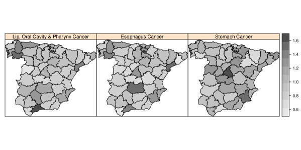
Figure 4: Standardized Mortality Ratio of lip, oral cavity and pharynx cancers, esophagus cancer and stomach cancer in Spain in 2013.

Figure 5 summarizes the estimates obtained with MCMC (Gibbs sampling with WinBUGS) and INLA within MCMC. In all plots, the solid lines represent the estimates of the posterior distribution using INLA within MCMC whilst the dashed lines is the estimate using MCMC. The top row shows the estimates of the posterior distribution of weights $\delta^{(d)}$ for the three diseases for which there is a very good agreement between both estimation methods. In the bottom line we can find the estimates of the common spatial effect, for which there is also good agreement between INLA within MCMC and MCMC.

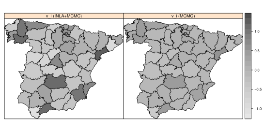
Figure 5: Summary of the posterior marginals of $\delta^{(d)}$ (top line) and the spatial common effect $v_{i}$ (bottom line). Solid lines represent estimates obtained with INLA within MCMC and the dashed line represents the marginals obtained with MCMC.

Finally, Figure 6 displays the marginal distributions of the disease specific intercepts $\alpha^{(d)}$ and precisions that appear in the model. These have been obtained by doing an average of the conditional marginals obtained at each step of the Metropolis-Hastings algorithm. In general, there is good agreement between our approach and MCMC.

Figure 6: Marginal distributions of the parameters in the model obtained by Bayesian model averaging the conditional marginals obtained at each step of the Metropolis-Hastings algorithm.

Although it is not shown here, we have observed a positive strong correlation between $\delta^{(1)}$ and $\delta^{(2)}$ We believe that this happens because of the similar spatial pattern that both diseases have. $\delta^{(3)}$ shows less correlation with the other two weighing parameters. This kind of multivariate inference has also been possible because we have been able to estimate the joint posterior distribution of $(\delta^{(1)},\delta^{(2)},\delta^{(3)})$ by fitting the model with INLA within MCMC.

6 Discussion

Gómez-Rubio and Rue [15] develop a novel approach to fit Bayesian models not implemented in the R-INLA by combining Metropolis-Hastings and INLA. In this paper we have exploited this method to show how to fit complex spatial models with several spatial components so that multivariate inference on a small ensemble of important parameters is feasible.

As seen in the examples presented in this paper, INLA within Metropolis can be used to fit complex spatial models with a simple implementation of the Metropolis-Hastings algorithm. This implementation is simpler compared to a full implementation of the model using several MCMC algorithms as sampling only involves a few parameters. Furthermore, convergence of the MCMC simulations is achieved in less iterations because the number of parameters that need to be simulated from is greatly reduced compared to fitting the model completely using MCMC. For large datasets, this should be an interesting alternative as INLA can fit conditional models faster than MCMC.

For cases in which the spatial model can be fitted completely with R-INLA, the approach presented in this paper is also appealing because it makes multivariate inference based on the joint posterior possible.

Bibliography

Bibliography

- Anselin [1988] Anselin, L. (1988). Spatial Econometrics: Methods and Models. Dordrecht: Kluwer.
- Besag et al. [1991] Besag, J., J. York, and A. Mollie (1991). Bayesian image restoration, with two applications in spatial statistics. Annals of the Institute of Statistical Mathematics 43(1), 1–59.
- Bivand and Piras [2015] Bivand, R. and G. Piras (2015). Comparing implementations of estimation methods for spatial econometrics. Journal of Statistical Software 63(1), 1–36.
- Bivand et al. [2014] Bivand, R. S., V. Gómez-Rubio, and H. Rue (2014). Approximate Bayesian inference for spatial econometrics models. Spatial Statistics 9, 146–165.
- Bivand et al. [2015] Bivand, R. S., V. Gómez-Rubio, and H. Rue (2015). Spatial data analysis with R-INLA with some extensions. Journal of Statistical Software 63(20), 1–31.
- Blangiardo and Cameletti [2015] Blangiardo, M. and M. Cameletti (2015). Spatial and Spatio-temporal Bayesian Models with R - INLA. John Wiley & Sons, Inc.
- Blangiardo et al. [2013] Blangiardo, M., M. Cameletti, G. Baio, and H. Rue (2013). Spatial and spatio-temporal models with R-INLA. Spatial and Spatio-Temporal Epidemiology 4, 33 – 49.
- Brooks et al. [2011] Brooks, S., A. Gelman, G. Jones, and X. Meng (Eds.) (2011). Handbook of Markov Chain Monte Carlo. Chapman & Hall/CRC Handbooks of Modern Statistical Methods. CRC Press.
- Cameletti et al. [2016] Cameletti, M., V. Gómez-Rubio, and M. Blangiardo (2016). Missing data analysis with the integrated nested laplace approximation. In preparation.
- Downing et al. [2008] Downing, A., D. Forman, M. S. Gilthorpe, K. L. Edwards, and S. O. Manda (2008). Joint disease mapping using six cancers in the yorkshire region of england. International Journal of Health Geographics 7(41), 1–14.
- Gilks et al. [1996] Gilks, W., W. Gilks, S. Richardson, and D. Spiegelhalter (1996). Markov Chain Monte Carlo in practice. Boca Raton, Florida: Chapman & Hall.
- Gómez-Rubio et al. [2014] Gómez-Rubio, V., R. S. Bivand, and H. Rue (2014). Spatial models using laplace approximation methods. In M. M. Fischer and P. Nijkamp (Eds.), Handbook of Regional Science, pp. 1401–1417. Berlin: Springer.
- Gómez-Rubio et al. [2016] Gómez-Rubio, V., R. S. Bivand, and H. Rue (2016). Estimating spatial econometrics models with integrated nested laplace approximation. In preparation.
- Gómez-Rubio et al. [2015] Gómez-Rubio, V., M. Cameletti, and F. Finazzi (2015). Analysis of massive marked point patterns with stochastic partial differential equations. Spatial Statistics B(14), 176–196.
- Gómez-Rubio and Rue [2016] Gómez-Rubio, V. and H. Rue (2016). Markov chain monte carlo with the integrated nested laplace approximation. In preparation.
- Gómez-Rubio et al. [2016] Gómez-Rubio, V., R. S. Bivand, and H. Rue (2016). Estimating spatial econometrics models with integrated nested laplace approximation. In preparation.
- Haining [2003] Haining, R. (2003). Spatial Data Analysis: Theory and Practice. Cambridge University Press.
- Hastings [1970] Hastings, W. K. (1970). Monte Carlo sampling methods using Markov chains and their applications. Biometrika 57, 97 – 109.
- Knorr-Held and Best [2001] Knorr-Held, L. and N. Best (2001). A shared component model for detecting joint and selective clustering of two diseases. Journal of the Royal Statistical Society, Series A 1(164), 73 – 85.
- Leroux et al. [1999] Leroux, B., X. Lei, and N. Breslow (1999). Estimation of disease rates in small areas: A new mixed model for spatial dependence. In M. Halloran and D. Berry (Eds.), Statistical Models in Epidemiology, the Environment and Clinical Trials, pp. 135–178. New York: Springer-Verlag.
- LeSage and Pace [2009] LeSage, J. and R. K. Pace (2009). Introduction to Spatial Econometrics. Chapman and Hall/CRC.
- Li et al. [2012] Li, Y., P. Brown, H. Rue, M. al-Maini, and P. Fortin (2012). Spatial modelling of Lupus incidence over 40 years with changes in census areas. Journal of the Royal Statistical Society, Series C 61, 99–115.
- Lindgren and Rue [2015] Lindgren, F. and H. Rue (2015). Bayesian spatial modelling with r-inla. Journal of Statistical Software 63(1), 1–25.
- Lindgren et al. [2011] Lindgren, F., H. Rue, and J. Lindstrom (2011). An explicit link between Gaussian fields and Gaussian Markov random fields: the stochastic partial differential equation approach. Journal of the Royal Statistical Society, Series B 73(Part 4), 423–498.
- Manski [1993] Manski, C. F. (1993). Identification of endogenous social effects: the reflection problem. Review of Economic Studies 60(3), 531–542.
- Martins et al. [2013] Martins, T. G., D. Simpson, F. Lindgren, and H. Rue (2013). Bayesian computing with INLA: New features. Computational Statistics & Data Analysis 67, 68–83.
- Metropolis et al. [1953] Metropolis, N., A. W. Rosenbluth, M. N. Rosenbluth, A. H. Teller, and E. Teller (1953). Equations of state calculations by fast computing machine. Journal of Chemical Physics 21, 1087 – 1091.
- Plummer [2016] Plummer, M. (2016). rjags: Bayesian Graphical Models using MCMC. R package version 4-6.
- R Core Team [2016] R Core Team (2016). R: A Language and Environment for Statistical Computing. Vienna, Austria: R Foundation for Statistical Computing.
- Rue and Held [2005] Rue, H. and L. Held (2005). Gaussian Markov Random Fields. Theory and Applications. Chapman & Hall/CRC.
- Rue et al. [2009] Rue, H., S. Martino, and N. Chopin (2009). Approximate Bayesian inference for latent Gaussian models by using integrated nested Laplace approximations. Journal of the Royal Statistical Society, Series B 71(Part 2), 319–392.
- Simpson et al. [2016] Simpson, D., J. B. Illian, F. Lindgren, S. H. Sørbye, and H. Rue (2016). Going off grid: computationally efficient inference for log-gaussian cox processes. Biometrika (To appear).
- Thomas et al. [2004] Thomas, A., N. Best, D. Lunn, R. Arnold, and D. Spiegelhalter (2004). GeoBUGS user manual.
- Ugarte et al. [2014] Ugarte, M. D., A. Adin, T. Goicoa, and A. F. Militino (2014). On fitting spatio-temporal disease mapping models using approximate bayesian inference. Statistical Methods in Medical Research 23(6), 507–530.