On the kinetic equation in Zakharov’s wave turbulence theory for capillary waves

Abstract

The wave turbulence equation is an effective kinetic equation that describes the dynamics of wave spectrum in weakly nonlinear and dispersive media. Such a kinetic model has been derived by physicists in the sixties, though the well-posedness theory remains open, due to the complexity of resonant interaction kernels. In this paper, we provide a global unique radial strong solution, the first such a result, to the wave turbulence equation for capillary waves.

Keyword: weak turbulence theory, capillary waves, water waves system, fluids mechanics

MSC: 35B05, 35B60, 82C40

1 Introduction

Over the last 60 years the theory of weak turbulence has been intensively developed. In weakly nonlinear and dispersive wave models, the weak turbulence kinetic equation can be formally derived, via the statistical approach, to describe the dynamics of resonant wave interactions. The model for slightly viscous capillary waves on the surface of a liquid reads as follows (cf. [30, 31, 41, 43])

$$\partial_{t}f+2\nu|k|^{2}f\ = \ Q[f]$$ (1.1)

in which $f(t,k)$ is the nonnegative wave density at wavenumber $k\in\mathbb{R}^{d}$, $d\geq 2$. Here, $\nu$ denotes the positive coefficient of fluid viscosity (strictly speaking, the model is derived under the assumption $\nu\sqrt{k}\ll 1$ so that the dispersion remains dominating the viscous dissipation; see [9] for more details on the addition of the viscous damping). The term $Q[f]$ denotes the integral collision operator, describing pure resonant three-wave interactions. The equation is a three-wave kinetic one, in which the collision operator is of the form

$$Q[f](k)\ =\ \iint_{\mathbb{R}^{2d}}\Big{[}R_{k,k_{1},k_{2}}[f]-R_{k_{1},k,k_{2}}[f]-R_{k_{2},k,k_{1}}[f]\Big{]}dk_{1}dk_{2}$$ (1.2)

with

$$R_{k,k_{1},k_{2}}[f]:=4\pi|V_{k,k_{1},k_{2}}|^{2}\delta(k-k_{1}-k_{2})\delta(\mathcal{E}_{k}-\mathcal{E}_{k_{1}}-\mathcal{E}_{k_{2}})(f_{1}f_{2}-ff_{1}-ff_{2})$$

with the short-hand notation $f=f(t,k)$ and $f_{j}=f(t,k_{j})$. The Dirac delta function $\delta(\cdot)$ is to ensure the following resonant conditions for the wavenumbers:

$$k=k_{1}+k_{2},\qquad\mathcal{E}_{k}=\mathcal{E}_{k_{1}}+\mathcal{E}_{k_{2}},$$ (1.3)

with $\mathcal{E}_{k}$ denoting the dispersion relation of the waves. The exact form of the collision kernel $V_{k,k_{1},k_{2}}$ will be recalled below.

According to the weak turbulence theory (cf. [43, 44, 23]), equation (1.1) in the absence of viscosity admits nontrivial equilibria $f_{\infty}$, called the Kolmogorov-Zakharov’s spectra:

$$f_{\infty}(k)\approx C|k|^{-\frac{17}{4}}.$$

Moreover, such a solution can be interpreted as a universal spectrum in the region of transparency. These solutions are the analogs of the familiar Kolmogorov energy spectrum prediction $C|k|^{-\frac{5}{3}}$ of hydrodynamic turbulence.

The derivation of the equation dated back to the 60’s, starting with the pioneering work of Hasselmann, Zakharov and collaborators (cf. [18, 19, 40, 41, 43]). Since then, a lot works have been done, trying to understand the equation (see [40, 23, 13, 17, 42, 41, 44, 7, 43, 28, 2, 30, 31, 12, 5, 15, 4, 16, 11, 34, 33, 25] and references therein). We refer to the books [27] for more discussions and references on the topic. Due to its complexity, the fundamental question on the global existence and uniqueness of solutions to the equation is still unsolved. In this paper, we give, for the first time, an answer to the fundamental question on the global existence and uniqueness of solutions to the equation, for the case where the solutions are radial.

In this paper, we develop new techniques, inspired by recent works on quantum kinetic theory. Let us mention that the kinetic wave equation (1.1) has a very similar structure with the quantum Boltzmann equation that describes the evolution of the excitations in a trapped Bose gas system, in which the temperature of the gas is below the Bose-Einstein condensate transition temperature (cf. [39, 45, 24, 21, 14, 22]). The collision operator that describes the interaction between excitations and condensates in the quantum Boltzmann equation reads

$$C[f](k)\ =\ \iint_{\mathbb{R}^{2d}}\Big{[}\bar{R}_{k,k_{1},k_{2}}[f]-\bar{R}_{k_{1},k,k_{2}}[f]-\bar{R}_{k_{2},k,k_{1}}[f]\Big{]}dk_{1}dk_{2}$$ (1.4)

with

$$\bar{R}_{k,k_{1},k_{2}}[f]:=|\bar{V}_{k,k_{1},k_{2}}|^{2}\delta(k-k_{1}-k_{2})\delta(\bar{\mathcal{E}}_{k}-\bar{\mathcal{E}}_{k_{1}}-\bar{\mathcal{E}}_{k_{2}})(f_{1}f_{2}-ff_{1}-ff_{2}-f)$$ (1.5)

and $|\bar{V}_{k,k_{1},k_{2}}|^{2}=\mathcal{C}^{*}|k||k_{1}||k_{2}|$, $\bar{\mathcal{E}}_{k}=\sqrt{\kappa_{1}|k|^{2}+\kappa_{2}|k|^{4}}$ for some positive constants $\mathcal{C}^{*},$ $\kappa_{1},$ $\kappa_{2}$. Recent progresses on quantum Boltzmann equations (cf. [10, 29, 36, 35, 1, 20, 32]) have opened some opportunities to tackle this open problem, the existence and uniqueness of solutions to (1.1).

We note that, in the absence of the linear term in (1.5) or the viscous damping in (1.1), singularities are likely to form. Indeed, [37] constructed a self-similar blowup solution to the quantum Boltzmann equation, when the linear term is dropped.

1.1 Main result

Throughout the paper, we consider the following generalized version of (1.1)

$$\partial_{t}f+2\nu(|k|^{2}+\varrho|k|^{4})f\ = \ Q[f]$$ (1.6)

for $\varrho\geq 0$. Solutions to the original model (1.1) will be obtained via the limit of $\varrho\to 0$.

The law of wave dispersion on the surface of infinitely deep liquid is of the form

$$\mathcal{E}_{k}=\sqrt{\sigma|k|^{3}}$$ (1.7)

for $\sigma$ the surface tension coefficient, and the collision kernel $V_{k,k_{1},k_{2}}$ is defined by

$$V_{k,k_{1},k_{2}}\ =\frac{1}{8\pi\sqrt{2\sigma}}\sqrt{\mathcal{E}_{k}\mathcal{E}_{k_{1}}\mathcal{E}_{k_{2}}}\Big{(}\frac{L_{k_{1},k_{2}}}{|k|\sqrt{|k_{1}||k_{2}|}}-\frac{L_{k,-k_{1}}}{|k_{2}|\sqrt{|k||k_{1}|}}-\frac{L_{k,-k_{2}}}{|k_{1}|\sqrt{|k||k_{2}|}}\Big{)}$$ (1.8)

with $L_{k_{1},k_{2}}=k_{1}\cdot k_{2}+|k_{1}||k_{2}|$; see [30, 31]. Without loss of generality, we assume the surface tension $\sigma=1$. In the scope of our paper, we only consider the case $d=2$ or $3$, which are relevant dimensions in the physical applications.

We shall construct global unique radial solutions to (1.6) in weighted $L^{1}$ spaces. Precisely, for $N>0$, let $L^{1}_{N}(\mathbb{R}^{d})$ be the function space consisting of $f(k)$ so that the norm

$$\|f\|_{L^{1}_{N}}:=\int_{\mathbb{R}^{d}}f(k)\mathcal{E}_{k}^{N}\;dk$$

is finite, with the dispersion relation $\mathcal{E}_{k}$ defined as in (1.7). In addition, for any $N>0$ and $\vartheta_{0}>0$, we introduce

$$\mathcal{S}_{N}:=\Big{\{}f\in L_{\frac{1}{3}}^{1}(\mathbb{R}^{d})\cap L_{N+3}^{1}(\mathbb{R}^{d})~{}:~{}f\geq 0,\quad f(k)=f(|k|),\qquad\|f\|_{L^{1}_{1}}+\|f\|_{L^{1}_{N+3}}\leq\vartheta_{0}\Big{\}}.$$

We shall construct solutions of (1.6) that remain $\mathcal{S}_{N}$, if initially so.

Our main result is as follows.

Theorem 1.1

Let $N>0$, and let $f_{0}(k)=f_{0}(|k|)\in\mathcal{S}_{N}\cap L^{2}(\mathbb{R}^{d})$, $d=2$ or $3$. Then for all $\varrho\geq 0$, the weak turbulence equation (1.6), with initial data $f(0,k)=f_{0}(k)$ and $\nu>0$, has a unique global solution $f(t,k)$ so that

$$0\leq f(t,k)=f(t,|k|)\in\mathcal{C}\big{(}[0,\infty);\mathcal{S}_{N}\cap L^{2}(\mathbb{R}^{d})\big{)}\cap\mathcal{C}^{1}\big{(}(0,\infty);L^{1}_{N}\big{)}.$$ (1.9)

Moreover, there holds the propagation of moments: for any $n\geq 1$, if $f_{0}\in L^{1}_{n}$, then there exists $C_{n}>0$ such that

$$\sup_{t\geq 0}\|f(t,\cdot)\|_{L^{1}_{n}}\leq C_{n}.$$ (1.10)

Remark 1.1

Notice that for the case where $\varrho>0$, we have a stronger result: we can remove the $L^{2}$ dependence on the initial condition, and the solution exists in $\mathcal{C}\big{(}[0,\infty);\mathcal{S}_{N}\cap L^{1}(\mathbb{R}^{d})\big{)}\cap\mathcal{C}^{1}\big{(}(0,\infty);L^{1}_{N}\big{)}$.

Let us mention that the classical Boltzmann equation describes the evolution of the density function of a dilute classical gas. After the collision, two particles with velocities $k_{1}$ and $k_{2}$ change their velocities into $k_{3}$ and $k_{4}$. Since the energy of the particles is of the form $\mathcal{E}_{k}=|k|^{2}$; the conservation of moment and energy then read

$$|k_{1}|^{2}+|k_{2}|^{2}=|k_{3}|^{2}+|k_{4}|^{2},\ \ \ k_{1}+k_{2}=k_{3}+k_{4}.$$

As a consequence, $k_{1}$, $k_{2}$, $k_{3}$, $k_{4}$ belong to the sphere centered at $\frac{k_{1}+k_{2}}{2}$ with radius $\frac{|k_{1}-k_{2}|}{2}$ and the classical Boltzmann collision operator can be expressed as a integration on a sphere (cf. [6, 38]).

Let us now turn to the collision operator of (1.6). As in the classical case, the collision operator involves surface integrals. Precisely, we introduce functions

$$H_{0}^{k}(w):=\mathcal{E}_{k-w}+\mathcal{E}_{w}-\mathcal{E}_{k},\ \ \ H_{1}^{k}(w):=\mathcal{E}_{k}+\mathcal{E}_{w}-\mathcal{E}_{k+w},$$ (1.11)

and the energy surfaces, dictated by the resonant conditions (1.3),

$$S_{k}: =\Big{\{}w\in\mathbb{R}^{d}~{}:~{}H^{0}_{k}(w)=0\Big{\}}$$ (1.12)

$$S^{\prime}_{k}: =\Big{\{}w\in\mathbb{R}^{d}~{}:~{}H^{1}_{k}(w)=0\Big{\}}$$

with $\mathcal{E}_{k}=\sqrt{\sigma}|k|^{3/2}$. The collision operator $Q[f]$ then reduces to

$$Q[f](k)=\int_{S_{k}}R_{k,k-k_{2},k_{2}}[f]\frac{d\sigma(k_{2})}{|\nabla H_{0}^{k}(k_{2})|}-2\int_{S^{\prime}_{k}}R_{k+k_{2},k,k_{2}}[f]\frac{d\sigma(k_{2})}{|\nabla H_{1}^{k}(k_{2})|}.$$ (1.13)

Difficulties arise. First, surfaces $S_{k}$ and $S_{k}^{\prime}$ are no longer a sphere as in the classical case, and the analysis on these surfaces can be tricky. More seriously, due to the lack of an integration over the whole space (compare with the classical Boltzmann equation), we are forced to bound surface integrals in term of (weighted) $L^{1}$ norms of solutions, a type of estimates that are in general false. In Section 2.2, we shall derive such estimates for radial functions.

By view of (1.3), the weak turbulence equation (1.6) conserves momentum and energy (in the absence of viscous damping), but does not conserve mass. As a consequence, one of the issues in dealing with (1.6) is that $L^{1}$ norms, say with weight $|k|^{n}$, of solutions do not close by itself, but are bounded by $L^{1}$ norms with a much higher-order weight. This is due to the high-order collision kernel. That is, roughly speaking, the kernel $|V_{k,k_{1},k_{2}}|^{2}$ is of order $9/2$ in $|k|$, which is much higher than the order of classical Boltzmann collision kernel (typically, smaller than one). This apparent loss of weights in $|k|$ gives the impression that solutions could blow up in finite time, even in the presence of viscous damping: $2\nu|k|^{2}f$, which gains precisely two order in $|k|$.

We end the introduction by giving the structure of the paper:

• We derive the momentum and energy identities and provide a careful study of the surface integrals on the energy manifolds.

• In Section 3, we provide an a priori estimate on the $L^{1}_{N}$ norm of the solution.

• An $L^{2}$ estimate on the solutions of (1.6) and the Hölder continuity of the collision operator will be established in Sections 4 and 5, respectively.

• The proof of Theorem 1.1 is given in Section 6.

2 Conservation laws and energy surfaces

2.1 Momentum and energy identity

In this section, we obtain the basic properties of strong solutions of (1.6).

Lemma 2.1

There holds

$$\int_{\mathbb{R}^{d}}Q[f](t,k)\varphi(k)\;dk\ = \ \iiint_{\mathbb{R}^{3d}}R_{k,k_{1},k_{2}}[f]\Big{[}\varphi(k)-\varphi(k_{1})-\varphi(k_{2})\Big{]}dkdk_{1}dk_{2}$$

for any test functions $\varphi$ so that the integrals make sense.

Proof  By definition, we compute

$$\int_{\mathbb{R}^{d}}Q[f](t,k)\varphi(k)\;dk\ = \ \iiint_{\mathbb{R}^{3d}}\Big{[}R_{k,k_{1},k_{2}}-R_{k_{1},k,k_{2}}-R_{k_{2},k,k_{1}}\Big{]}\varphi(k)dkdk_{1}dk_{2}.$$

By switching the variables $k\leftrightarrow k_{1}$, $k\leftrightarrow k_{2}$ in the first integral on the right, the lemma follows at once.  

As a direct consequence, we obtain the following corollary.

Corollary 2.1 (Momentum and energy identities)

Smooth solutions $f(t,k)$ of (1.6) satisfy

$$\frac{d}{dt}\int_{\mathbb{R}^{d}}f(t,k)kdk+2\nu\int_{\mathbb{R}^{d}}f(t,k)k(|k|^{2}+\varrho|k|^{4})dk=0$$ (2.1)

and

$$\frac{d}{dt}\int_{\mathbb{R}^{d}}f(t,k)\mathcal{E}_{k}dk+2\nu\int_{\mathbb{R}^{d}}f(t,k)\mathcal{E}_{k}(|k|^{2}+\varrho|k|^{4})dk=0$$ (2.2)

for all $t\geq 0$.

Proof  This follows from Lemma 2.1 by taking $\varphi(k)=k$ and $\varphi(k)=\mathcal{E}_{k}$, and using the resonant conditions (1.3).  

2.2 Energy surfaces

Our first step is to study the surface integrals. For sake of generality, we consider in this section the following power-law energy function

$$\mathcal{E}_{k}=\mathcal{E}(k)=|k|^{\gamma},\qquad 1<\gamma\leq 2.$$ (2.3)

In the case when $\gamma=1$, the surface $S_{k}$ degenerates into a straight line $S_{k}=\{\alpha k\}_{\alpha\in[0,1]}$, and the surface integral reduces to a line integral. Such an energy corresponds to the dispersion law of phonons, and has been studied in [1, 8, 10].

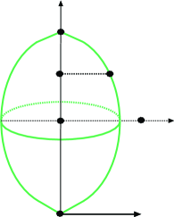
Figure 1: Sketched is the surface $S_{p}$, centered at $\frac{p}{2}$ and having $0$ and $p$ as its south and north poles, respectively.

Lemma 2.2 (Surface $S_{p}$)

Let $\gamma\in(1,2]$ and $S_{p}$ be defined as in (1.12)-(2.3). Then, for each $p$, $S_{p}=|p|S_{e_{p}}$, with $e_{p}=p/|p|$. In addition, there hold the following properties:

i. $\{0,p\}\subset S_{p}\subset\overline{B(\frac{p}{2},\frac{|p|}{2})}$.

ii. The surface $S_{p}$ is invariant under the rotation around $p$, and can be parametrized by

$$S_{p}=\Big{\{}w(\alpha,e_{q})=\alpha p+s(\alpha)e_{q}~{}:~{}\alpha\in[0,1],\quad|e_{q}|=1,\quad e_{q}\cdot p=0\Big{\}}$$

for some function $s(\alpha)$ that is smooth in $(0,1)$; see Figure 1. In the two dimensional case: $d=2$, $S_{p}$ is a curve parametrized by $\alpha\in[0,1]$.

iii. $s(\alpha)=s(1-\alpha)$, $s(0)=0$, and $s(\alpha)$ is strictly increasing and invertible on $(0,\frac{1}{2})$.

iv. There are universal constants $c_{0},C_{0}$ so that the surface area satisfies

$$c_{0}|p|^{d-\gamma}\leq\int_{S_{p}}\frac{d\sigma(w)}{|\nabla_{w}H_{0}^{p}(w)|}\leq C_{0}|p|^{d-\gamma},$$

uniformly in $p\in\mathbb{R}^{d}$.

v. There holds

$$\int_{S_{p}}F(|w|)\frac{d\sigma(w)}{|\nabla_{w}H_{0}^{p}(w)|}\leq C|p|^{d-\gamma-2}\int_{|w|\leq|p|}F(|w|)|w|^{2-d}dw.$$

Proof  Let $p\in\mathbb{R}^{d}\setminus\{0\}$. It is clear that $S_{p}=|p|S_{e_{p}}$, with $e_{p}=p/|p|$. Thus, it suffices to study the case when $|p|=1$. As for (i), it is clear that $\{0,p\}\subset S_{p}$. Next, since $a^{\gamma}+b^{\gamma}\leq(a+b)^{\gamma}$, we have for $w\in S_{p}$

$$1=\Big{(}|p-w|^{\gamma}+|w|^{\gamma}\Big{)}^{2/\gamma}\geq|p-w|^{2}+|w|^{2}.$$

This proves that $w\in\overline{B(\frac{p}{2},\frac{1}{2})}$. (i) follows.

As for (ii), we write $w=\alpha p+q$ for $q$ orthogonal to $p$. By orthogonality, $|w|$ and $|w-p|$ do not depend on the direction of $q$, and neither does $S_{p}$. That is, $S_{p}$ is invariant under the rotation around $p$. We set

$$w(\alpha,s)=\alpha p+se_{q}.$$

We shall prove the existence of a function $s=s(\alpha)$ for $\alpha\in(0,1)$, so that $w(\alpha,s(\alpha))\in S_{p}$. To this end, let

$$H_{0}^{p}(\alpha,s):=\mathcal{E}(p-w(\alpha,s))+\mathcal{E}(w(\alpha,s))-\mathcal{E}(p),$$

as in (1.11). Clearly, $H_{0}^{p}(\alpha,s)=0$ if and only if $w(\alpha,s)\in S_{p}$. Observe that $H_{0}^{p}(\alpha,0)<0$ (by convexity of $\mathcal{E}(p)$) and $H_{0}^{p}(\alpha,s)>0$ for sufficiently large $s$ (and hence large $|w(\alpha,s)|)$. The existence of a such $s(\alpha)$ follows. In addition, a direct computation yields

$$\nabla_{w}H_{0}^{p} =\frac{w-p}{|p-w|}\mathcal{E}^{\prime}(p-w)+\frac{w}{|w|}\mathcal{E}^{\prime}(w)$$ (2.4)

and hence $\partial_{s}H_{0}^{p}(\alpha,s)=e_{q}\cdot\nabla_{w}H_{0}^{p}$ is positive, since $\mathcal{E}^{\prime}(w)>0$ (for $w\not=0$). That is, $H_{0}^{p}(\alpha,s)$ is increasing in $s$ for each $\alpha$ and $s(\alpha)$ is uniquely determined, so that $H_{0}^{p}(\alpha,s(\alpha))=0$. The smoothness of $s(\alpha)$ follows from that of $\mathcal{E}(\cdot)$. This proves (ii).

Next, the symmetry stated in (iii) is clear from the definition of $S_{p}$, and it suffices to study $s(\alpha)$ for $\alpha\in(0,\frac{1}{2}]$. Observe that for $w_{\alpha}=w(\alpha,s(\alpha))\in S_{p}$, we have $0=F(\alpha,s(\alpha))$ and

$$0 =\partial_{\alpha}H_{0}^{p}+s^{\prime}(\alpha)\partial_{s}H_{0}^{p}=p\cdot\nabla_{w}H_{0}^{p}+s^{\prime}(\alpha)e_{q}\cdot\nabla_{w}H_{0}^{p}$$ (2.5)

$$=-\frac{\mathcal{E}^{\prime}(p-w_{\alpha})}{|p-w_{\alpha}|}+(s(\alpha)s^{\prime}(\alpha)+\alpha)\Big{[}\frac{\mathcal{E}^{\prime}(p-w_{\alpha})}{|p-w_{\alpha}|}+\frac{\mathcal{E}^{\prime}(w_{\alpha})}{|w_{\alpha}|}\Big{]}.$$

Setting $\mathcal{E}_{1}(w):=|w|^{\gamma-2}$, we have

$$s(\alpha)s^{\prime}(\alpha)=\frac{(1-\alpha)\mathcal{E}_{1}(p-w_{\alpha})-\alpha\mathcal{E}_{1}(w_{\alpha})}{\mathcal{E}_{1}(p-w_{\alpha})+\mathcal{E}_{1}(w_{\alpha})}.$$ (2.6)

Observe that the function in the numerator in (2.6) is decreasing in $\alpha$, and vanishes at $\alpha=\frac{1}{2}$. Hence, for $\alpha\in(0,\frac{1}{2})$, we have $s^{\prime}(\alpha)>0$, and hence $s(\alpha)$ is invertible, on $(0,\frac{1}{2})$. This yields (iii).

Next, we compute the surface area of $S_{p}$. Let us consider the case when $d\geq 3$; the case when $d=2$ is simpler, as the surface is parametrized solely by $\alpha\in[0,1]$. Writing $w(\alpha,\theta)=\alpha p+s(\alpha)e_{\theta}$, we have

$$d\sigma(w) =|\partial_{\alpha}w\times\partial_{\theta}w|d\alpha d\theta=\Big{|}(p+s^{\prime}(\alpha)e_{\theta})\times s(\alpha)\partial_{\theta}e_{\theta}\Big{|}d\alpha d\theta$$ (2.7)

$$=\sqrt{|p|^{2}|s(\alpha)|^{2}+\frac{1}{4}|\partial_{\alpha}(|s(\alpha)|^{2})|^{2}}d\alpha d\theta.$$

We deduce from (2.5) that

$$0 =\partial_{\alpha}w_{\alpha}\cdot\nabla_{w}H_{0}^{p}$$ (2.8)

$$=\frac{1}{2}\partial_{\alpha}|s(\alpha)|^{2}\left[\frac{\mathcal{E}^{\prime}(|p-w_{\alpha}|)}{|p-w_{\alpha}|}+\frac{\mathcal{E}^{\prime}(|w_{\alpha}|)}{|w_{\alpha}|}\right]+\alpha|p|^{2}\frac{\mathcal{E}^{\prime}(|w_{\alpha}|)}{|w_{\alpha}|}-(1-\alpha)|p|^{2}\frac{\mathcal{E}^{\prime}(|p-w_{\alpha}|)}{|p-w_{\alpha}|}.$$

It is straightforward that

$$\partial_{\alpha}|s(\alpha)|^{2} =2|p|^{2}\frac{\gamma\frac{\mathcal{E}^{\prime}(|w_{\alpha}|)}{|w_{\alpha}|}+(\alpha-1)\frac{\mathcal{E}^{\prime}(|p-w_{\alpha}|)}{|p-w_{\alpha}|}}{\frac{\mathcal{E}^{\prime}(|p-w_{\alpha}|)}{|p-w_{\alpha}|}+\frac{\mathcal{E}^{\prime}(w_{\alpha})}{|w_{\alpha}|}}.$$ (2.9)

Now, let us compute $|\nabla H_{0}^{p}|$ under the new parametrization

$$|\nabla H_{0}^{p}|^{2}\ = \ |p|^{2}\left[\alpha\frac{\mathcal{E}^{\prime}(|w_{\alpha}|)}{|w_{\alpha}|}+(\alpha-1)\frac{\mathcal{E}^{\prime}(|p-w_{\alpha}|)}{|p-w_{\alpha}|}\right]^{2}$$

$$\ +|s(\alpha)|^{2}\left[\frac{\mathcal{E}^{\prime}(|p-w_{\alpha}|)}{|p-w_{\alpha}|}+\frac{\mathcal{E}^{\prime}(|w_{\alpha}|)}{|w_{\alpha}|}\right]^{2},$$

which, in companion with (2.9), implies

$$|\nabla H_{0}^{p}|^{2}\ = \ \frac{\left|\partial_{\alpha}|s(\alpha)|^{2}\right|^{2}}{4|p|^{2}}\left[\frac{\mathcal{E}^{\prime}(|p-w_{\alpha}||)}{|p-w_{\alpha}||}+\frac{\mathcal{E}^{\prime}(|w_{\alpha}||)}{|w_{\alpha}||}\right]^{2}$$ (2.10)

$$\ +|s(\alpha)|^{2}\left[\frac{\mathcal{E}^{\prime}(|p-w_{\alpha}|)}{|p-w_{\alpha}|}+\frac{\mathcal{E}^{\prime}(|w_{\alpha}|)}{|w_{\alpha}|}\right]^{2},$$

We get the following representation of $|\nabla H_{0}^{p}|$

$$|\nabla H_{0}^{p}|\ = \ \frac{\sqrt{\frac{\left|\partial_{\alpha}|s(\alpha)|^{2}\right|^{2}}{4}+|\alpha|^{2}|p|^{2}}}{|p|}\left[\frac{\mathcal{E}^{\prime}(|p-w_{\alpha}|)}{|p-w_{\alpha}|}+\frac{\mathcal{E}^{\prime}(|w_{\alpha}|)}{|w_{\alpha}|}\right].$$ (2.11)

As for the surface integral of a radial function $\mathcal{G}(|w|)$, we introduce the radial variable $u=|W_{\alpha}|=\sqrt{\alpha^{2}|p|^{2}+|q_{\alpha}|^{2}}$. We compute $2udu=\partial_{\alpha}|W_{\alpha}|^{2}d\alpha$ and hence

$$\frac{d\sigma(w)}{|\nabla H_{0}^{p}|}=\frac{|p|}{2\left[\frac{\mathcal{E}^{\prime}(|p-w_{\alpha}|)}{|p-w_{\alpha}|}+\frac{\mathcal{E}^{\prime}(|w_{\alpha}|)}{|w_{\alpha}|}\right]\partial_{\alpha}|w_{\alpha}|^{2}}udud\theta,$$

which in combination with (2.8) yields

$$\frac{d\sigma(w)}{|\nabla H_{0}^{p}|}=\frac{|p-w_{\alpha}|}{\mathcal{E}^{\prime}(|p-w_{\alpha}|)|p|}dud\theta=\frac{u|p-w_{\alpha}|^{2-\gamma}}{|p|(\gamma-1)}dud\theta,$$

Since

$$\frac{u||p|+u|^{2-\gamma}}{|p|(\gamma-1)}\leq\frac{u|p-w_{\alpha}|^{2-\gamma}}{|p|(\gamma-1)}\leq\frac{u[|p|+u]^{2-\gamma}}{|p|(\gamma-1)},$$

upon noting that $d\sigma(S_{p})=|p|^{d-1}d\sigma(S_{e_{p}})$ and defining $v=\frac{u}{|p|}$, we obtain

$$\int_{S_{p}}\frac{d\sigma(w)}{|\nabla_{w}H_{0}^{p}|}\geq c_{1}|p|^{d-\gamma}\int_{0}^{1}v|1-v|^{2-\gamma}dv\geq c_{0}|p|^{d-\gamma},$$

and

$$\int_{S_{p}}\frac{d\sigma(w)}{|\nabla_{w}H_{0}^{p}|})\leq C_{1}|p|^{d-\gamma}\int_{0}^{1}v|1+v|^{2-\gamma}dv\leq C_{0}|p|^{d-\gamma},$$

for some $c_{0},c_{1},$ $C_{0},C_{1}$, depending only on $\gamma$ (in particular, independent of $p$). This proves (iv).

Finally, we check the surface integral of a radial function $f(|w|)$. It is clear that

$$\int_{S_{p}}f(|w|)\frac{d\sigma(w)}{|\nabla H_{0}^{p}|}\leq C|p|^{d-\gamma-2}\int_{0}^{|p|}f(u)udu.$$

The lemma follows by the spherical coordinates $dw=|w|^{d-1}d(|w|)d\sigma(\mathbb{S}^{d}).$  

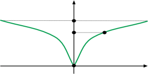
Figure 2: Sketched is the trace of $S^{\prime}_{p}$ on any two dimensional plane containing $p$.

Lemma 2.3 (Surface $S_{p}^{\prime}$)

Let $S_{p}^{\prime}$ be defined as in (1.12)-(2.3). Then, $S_{p}^{\prime}=|p|S^{\prime}_{e_{p}}$, with $e_{p}=p/|p|$. In addition, There is a positive constant $C_{0}$ so that

$$\int_{S_{p}^{\prime}}F(|w|)\;\frac{d\sigma(w)}{|\nabla_{w}H_{1}^{p}(w)|}\leq C_{0}|p|^{d-2-\gamma}\int_{0}^{\infty}F(|w|)(1+|w|/|p|)^{2-\gamma}|w|^{2-d}dw$$ (2.12)

uniformly in $p\in\mathbb{R}^{d}.$

Proof  It is clear that $S_{p}^{\prime}=|p|S_{e_{p}}^{\prime}$, in which the surface

$$S^{\prime}_{e_{p}}=\Big{\{}w(\alpha,\theta)=\alpha e_{p}+s(\alpha)e_{\theta}~{}:~{}\alpha\in[0,\alpha_{0}),~{}\theta\in[0,2\pi]\Big{\}}$$ (2.13)

for some monotonic function $s(\alpha)$ and some positive constant $\alpha_{0}$; see Figure 2. We stress that the parametrization $\alpha,s(\alpha)$ and $\theta$ are independent of $p$. As a consequence, the surface integral on $S^{\prime}_{e_{p}}$ is independent of $p$.

As in (2.7), we have

$$d\sigma(w)=\sqrt{|p|^{2}|s(\alpha)|^{2}+\frac{1}{4}|\partial_{\gamma}(|s(\alpha)|^{2})|^{2}}d\alpha d\theta$$

and hence, the surface is estimated by

$$\frac{d\sigma(w)}{|\nabla H_{1}^{p}(w)|} =\frac{\sqrt{|p|^{2}|s(\alpha)|^{2}+\frac{1}{4}|\partial_{\alpha}(|s(\alpha)|^{2})|^{2}}}{|\nabla H_{1}^{p}(|\alpha p+s(\alpha)|)|}d\alpha d\theta.$$

Let us introduce the variable $u=|w|=\sqrt{\alpha^{2}|p|^{2}+|s(\alpha)|^{2}}$. We compute

$$2udu=\partial_{\alpha}|w_{\alpha}|^{2}d\alpha$$

and hence

$$\frac{d\sigma(w)}{|\nabla H_{1}^{p}(w_{\alpha})|}\;=C\frac{\sqrt{|p|^{2}|s(\alpha)|^{2}+\frac{1}{4}|\partial_{\alpha}(|s(\alpha)|^{2})|^{2}}}{2\partial_{\alpha}|w_{\alpha}|^{2}|\nabla H_{1}^{p}(|\alpha p+s(\alpha)|)|}udud\theta.$$ (2.14)

We recall that $H_{1}^{p}(w_{\alpha})=0$ and hence

$$0=\partial_{\alpha}w_{\alpha}\cdot\nabla_{w}H_{1}^{p}=\frac{1}{2}\partial_{\alpha}|w_{\alpha}|^{2}\Big{[}\frac{\mathcal{E}^{\prime}(p+w_{\alpha})}{|p+w_{\alpha}|}-\frac{\mathcal{E}^{\prime}(w_{\alpha})}{|w_{\alpha}|}\Big{]}+|p|^{2}\frac{\mathcal{E}^{\prime}(p+w_{\alpha})}{|p+w_{\alpha}|}$$

which leads to

$$|p|^{2}\frac{\mathcal{E}^{\prime}(p+w_{\alpha})}{|p+w_{\alpha}|}=\frac{1}{2}\partial_{\alpha}|w_{\alpha}|^{2}\left[\frac{\mathcal{E}^{\prime}(w_{\alpha})}{|w_{\alpha}|}-\frac{\mathcal{E}^{\prime}(p+w_{\alpha})}{|p+w_{\alpha}|}\right],$$ (2.15)

and

$$\partial_{\alpha}|s(\alpha)|^{2}=2\frac{-\alpha|p|^{2}\frac{\mathcal{E}^{\prime}(|w_{\alpha}|)}{|w_{\alpha}|}+(1+\alpha)|p|^{2}\frac{\mathcal{E}^{\prime}(|p+w_{\alpha}|)}{|p+w_{\alpha}|}}{\left[\frac{\mathcal{E}^{\prime}(w_{\alpha})}{|w_{\alpha}|}-\frac{\mathcal{E}^{\prime}(p+w_{\alpha})}{|p+w_{\alpha}|}\right]}.$$ (2.16)

We deduce from (2.16) that

$$|\nabla H_{1}^{p}|^{2}\ = \ |p|^{2}\left[-\alpha\frac{\mathcal{E}^{\prime}(|w_{\alpha}|)}{|w_{\alpha}|}+(\alpha+1)\frac{\mathcal{E}^{\prime}(|p+w_{\alpha}|)}{|p+w_{\alpha}|}\right]^{2}\ +|s(\alpha)|^{2}\left[\frac{\mathcal{E}^{\prime}(|p+w_{\alpha}|)}{|p+w_{\alpha}|}-\frac{\mathcal{E}^{\prime}(|w_{\alpha}|)}{|w_{\alpha}|}\right]^{2}$$

$$= \ \frac{\left|\partial_{\gamma}|s(\alpha)|^{2}\right|^{2}}{4|p|^{2}}\left[\frac{\mathcal{E}^{\prime}(|p+w_{\alpha}|)}{|p+w_{\alpha}|}-\frac{\mathcal{E}^{\prime}(|w_{\alpha}|)}{|w_{\alpha}|}\right]^{2}\ +|s(\alpha)|^{2}\left[\frac{\mathcal{E}^{\prime}(|p+w_{\alpha}|)}{|p+w_{\alpha}|}-\frac{\mathcal{E}^{\prime}(|w_{\alpha}|)}{|w_{\alpha}|}\right]^{2},$$

which implies

$$\frac{d\sigma(w)}{|\nabla H_{1}^{p}(w)|}\;=C\frac{|p|}{\partial_{\alpha}|w_{\alpha}|^{2}\left[\frac{\mathcal{E}^{\prime}(|w_{\alpha}|)}{|w_{\alpha}|}-\frac{\mathcal{E}^{\prime}(|p+w_{\alpha}|)}{|p+w_{\alpha}|}\right]}udud\theta.$$

The above and (2.15) yield

$$\frac{d\sigma(w)}{|\nabla H_{1}^{p}(w)|}\;=C\frac{udu}{2|p|\frac{\mathcal{E}^{\prime}(|p+w|)}{|p+w|}}.$$

We the obtain

$$\int_{S_{p}^{1}}\frac{F(|w|)}{|\nabla H_{1}^{p}(w)|}\;d\sigma(w)=C|p|^{d-2-\gamma}\int_{0}^{\infty}F(u)(1+u/|p|)^{2-\gamma}du.$$

The lemma follows by the spherical coordinates $dw=|w|^{d-1}d(|w|)d\sigma(\mathbb{S}^{d}).$  

3 Weighted $L^{1}$ estimates

In this section, we shall derive uniform estimates on the weighted $L^{1}$ norm, where weights are $n^{th}$-order monomials of $\mathcal{E}_{k}$, which are defined by

$$\mathfrak{M}_{n}[g]=\int_{\mathbb{R}^{d}}\mathcal{E}^{n}_{k}g(k)dk$$ (3.1)

in which we recall the energy function $\mathcal{E}_{k}=|k|^{3/2}$. We stress that our estimates might depend on the positive coefficient of viscosity, but is independent of $\varrho$, in the equation; see (1.6).

3.1 Estimate of the collision operator

We first obtain the following estimate on the collision operator $Q[g]$.

Lemma 3.1

Let $N>1$. For any positive and radial function $g(p)=g(|p|)$, there exists a constant $C_{N}$, depending on $N$, such that the following holds

$$\int_{\mathbb{R}^{d}}Q[g](k)\mathcal{E}^{N}_{k}\;dk$$ (3.2)

$$\leq C_{N}\sum_{n=[N/2]}^{N-1}\Big{(}\mathfrak{M}_{n+\frac{7-2d}{3}}[g]\mathfrak{M}_{N-n+\frac{2d-1}{3}}[g]+\mathfrak{M}_{n+\frac{11-2d}{3}}[g]\mathfrak{M}_{N-n+\frac{2d-5}{3}}[g]\Big{)}.$$

Proof  It is sufficient to prove the lemma for $N$ to be natural numbers. By Lemma 2.1, we have

$$\int_{\mathbb{R}^{d}}Q[g](k)\mathcal{E}_{k}^{N}\;dk\ = \ \iiint_{\mathbb{R}^{3d}}R_{k,k_{1},k_{2}}[g]\Big{[}\mathcal{E}^{N}_{k}-\mathcal{E}^{N}_{k_{1}}-\mathcal{E}^{N}_{k_{2}}\Big{]}dkdk_{1}dk_{2}.$$

Using the resonant conditions $k=k_{1}+k_{2}$ and $\mathcal{E}_{k}=\mathcal{E}_{k_{1}}+\mathcal{E}_{k_{2}}$, dictated by the Dirac delta functions in $R_{k,k_{1},k_{2}}[g]$, we can write

$$\mathcal{E}_{k}^{N}-\mathcal{E}^{N}_{k_{1}}-\mathcal{E}^{N}_{k_{2}}=(\mathcal{E}_{k_{1}}+\mathcal{E}_{k_{2}})^{N}-\mathcal{E}^{N}_{k_{1}}-\mathcal{E}^{N}_{k_{2}}=\sum_{n=1}^{N-1}{{N}\choose{n}}\mathcal{E}^{n}_{k_{1}}\mathcal{E}^{N-n}_{k_{2}}.$$

Thus, we obtain

$$\int_{\mathbb{R}^{d}}Q[g](k)\mathcal{E}_{k}^{N}\;dk =\iint_{\mathbb{R}^{2d}}R_{k_{1}+k_{2},k_{1},k_{2}}[g]\sum_{n=1}^{N-1}{{N}\choose{n}}\mathcal{E}^{n}_{k_{1}}\mathcal{E}^{N-n}_{k_{2}}dk_{1}dk_{2}$$ (3.3)

$$=\iint_{\mathbb{R}^{2d}}R_{k_{1}+k_{2},k_{1},k_{2}}[g]\sum_{n=1}^{[N/2]-1}{{N}\choose{n}}\mathcal{E}^{n}_{k_{1}}\mathcal{E}^{N-n}_{k_{2}}dk_{1}dk_{2}$$

$$\quad+\iint_{\mathbb{R}^{2d}}R_{k_{1}+k_{2},k_{1},k_{2}}[g]\sum_{n=[N/2]}^{N-1}{{N}\choose{n}}\mathcal{E}^{n}_{k_{1}}\mathcal{E}^{N-n}_{k_{2}}dk_{1}dk_{2}$$

$$=:I_{1}+I_{2}.$$

Clearly, due to the symmetry of $k_{1}$ and $k_{2}$, it suffices to give estimates on $I_{2}$. Indeed, we write

$$I_{1} =\iint_{\mathbb{R}^{2d}}R_{k_{1}+k_{2},k_{1},k_{2}}[g]\sum_{n=N-[N/2]+1}^{N}{{N}\choose{N-n}}\mathcal{E}^{N-n}_{k_{1}}\mathcal{E}^{n}_{k_{2}}dk_{1}dk_{2},$$

which is in fact $I_{2}$. We now estimate $I_{2}$. Recall that

$$R_{k,k_{1},k_{2}}[g]=4\pi|V_{k,k_{1},k_{2}}|^{2}\delta(k-k_{1}-k_{2})\delta(\mathcal{E}_{k}-\mathcal{E}_{k_{1}}-\mathcal{E}_{k_{2}})(g_{1}g_{2}-gg_{1}-gg_{2})$$ (3.4)

and the energy surface $S_{k}^{\prime}$ is defined as in (1.12). Thus, using the nonnegativity of $g(k)$, we can drop the last two terms $gg_{1}+gg_{2}$ in (3.4), yielding

$$I_{2} \leq 4\pi\int_{\mathbb{R}^{d}}\int_{S_{k_{2}}^{\prime}}|V_{k_{1}+k_{2},k_{1},k_{2}}|^{2}g_{1}g_{2}\sum_{n=[N/2]}^{N-1}{{N}\choose{n}}\mathcal{E}^{n}_{k_{1}}\mathcal{E}^{N-n}_{k_{2}}\frac{d\sigma(k_{1})}{|\nabla H^{k_{2}}_{1}(k_{1})|}dk_{2},$$

in which $H_{1}^{k}$ is defined as in (1.11). Let us now estimate the collision kernel $V_{k_{1}+k_{2},k_{1},k_{2}}$, defined as in (1.8). We recall

$$V_{k,k_{1},k_{2}}\ =\frac{1}{8\pi\sqrt{2\sigma}}\sqrt{\mathcal{E}_{k}\mathcal{E}_{k_{1}}\mathcal{E}_{k_{2}}}\Big{(}\frac{L_{k_{1},k_{2}}}{|k|\sqrt{|k_{1}||k_{2}|}}-\frac{L_{k,-k_{1}}}{|k_{2}|\sqrt{|k||k_{1}|}}-\frac{L_{k,-k_{2}}}{|k_{1}|\sqrt{|k||k_{2}|}}\Big{)}$$

with $L_{k_{1},k_{2}}=k_{1}\cdot k_{2}+|k_{1}||k_{2}|$ and $\mathcal{E}_{k}=|k|^{3/2}$. It is clear that $|L_{k_{1},k_{2}}|\leq 2|k_{1}||k_{2}|$. In addition, the energy identity $\mathcal{E}_{k}=\mathcal{E}_{k_{1}}+\mathcal{E}_{k_{2}}$ in particular implies that $|k_{1}|\leq|k|$ and $|k_{2}|\leq|k|$, due to the monotonicity of $\mathcal{E}_{k}$. Hence, for $k=k_{1}+k_{2}$, we compute

$$0 \leq L_{k,-k_{1}}=|k||k_{1}|-k\cdot k_{1}=|k_{1}|(|k|-|k_{1}|)-k_{1}\cdot k_{2}\leq 2|k_{1}||k_{2}|.$$ (3.5)

The same bound holds for $L_{k,-k_{2}}$. This proves that

$$|V_{k,k_{1},k_{2}}|\leq C_{0}\sqrt{\mathcal{E}_{k}\mathcal{E}_{k_{1}}\mathcal{E}_{k_{2}}}\Big{(}\frac{\sqrt{|k_{1}||k_{2}|}}{|k|}+\frac{\sqrt{|k_{1}|}}{\sqrt{|k|}}+\frac{\sqrt{|k_{2}|}}{\sqrt{|k|}}\Big{)}$$

for some universal constant $C_{0}$. Using again $|k|\geq\max\{|k_{1}|,|k_{2}|\}$, we obtain

$$|V_{k,k_{1},k_{2}}|\leq C_{0}\sqrt{\mathcal{E}_{k}\mathcal{E}_{k_{1}}\mathcal{E}_{k_{2}}}$$ (3.6)

for all $(k,k_{1},k_{2})$ satisfying the resonant conditions $k=k_{1}+k_{2}$ and $\mathcal{E}_{k}=\mathcal{E}_{k_{1}}+\mathcal{E}_{k_{2}}$. Hence, we have

$$I_{2} \leq C_{0}\int_{\mathbb{R}^{d}}\int_{S_{k_{2}}^{\prime}}\mathcal{E}_{k_{1}}\mathcal{E}_{k_{2}}(\mathcal{E}_{k_{1}}+\mathcal{E}_{k_{2}})g_{1}g_{2}\sum_{n=[N/2]}^{N-1}{{N}\choose{n}}\mathcal{E}^{n}_{k_{1}}\mathcal{E}^{N-n}_{k_{2}}\frac{d\sigma(k_{1})}{|\nabla H^{k_{2}}_{1}(k_{1})|}dk_{2}$$

$$\leq C_{0}\sum_{n=[N/2]}^{N-1}{{N}\choose{n}}\int_{\mathbb{R}^{d}}g_{2}\mathcal{E}^{N-n+1}_{k_{2}}\Big{(}\int_{S_{k_{2}}^{\prime}}\mathcal{E}^{n+1}_{k_{2}}(\mathcal{E}_{k_{1}}+\mathcal{E}_{k_{2}})g_{1}\frac{d\sigma(k_{1})}{|\nabla H^{k_{2}}_{1}(k_{1})|}\Big{)}dk_{2}.$$

Next, applying Lemma 2.3, with $\gamma=3/2$, to the surface integral on $S_{k_{2}}^{\prime}$ and recalling that $g_{1}=g(|k_{1}|)$, we obtain

$$\int_{S_{k_{2}}^{\prime}}g_{1}\mathcal{E}^{n+1}_{k_{1}}(\mathcal{E}_{k_{1}}+\mathcal{E}_{k_{2}})\frac{d\sigma(k_{1})}{|\nabla H^{k_{2}}_{1}(k_{1})|}$$ (3.7)

$$\leq C_{0}\int_{\mathbb{R}^{d}}g(k)\mathcal{E}^{n+1}_{k_{1}}(\mathcal{E}_{k_{1}}+\mathcal{E}_{k_{2}})\mathcal{E}_{k_{2}}^{\frac{2(d-4)}{3}}(\mathcal{E}_{k_{1}}^{\frac{1}{3}}+\mathcal{E}_{k_{2}}^{\frac{1}{3}})\mathcal{E}_{k_{1}}^{\frac{2(2-d)}{3}}dk_{1}.$$

This proves

$$I_{2} \leq C_{N}\sum_{n=[N/2]}^{N-1}\Big{(}\mathfrak{M}_{n+1+\frac{4-2d}{3}}[g]\mathfrak{M}_{N-n+1+\frac{2d-4}{3}}[g]+\mathfrak{M}_{n+1+\frac{8-2d}{3}}[g]\mathfrak{M}_{N-n+1+\frac{2d-8}{3}}[g]\Big{)}.$$

This proves the lemma.  

Remark 3.1

We note that by writing $L_{k,-k_{1}}$ and $L_{k,-k_{2}}$ as in (3.5), the kernel $|V_{k,k_{1},k_{2}}|$ is radial in $k$.

3.2 Weighted $L^{1}_{N}$ $(N>1)$ estimates

Proposition 3.1

Let $N>1$. Suppose that $f_{0}(k)=f_{0}(|k|)$ is a nonnegative radial initial data satisfying

$$\int_{\mathbb{R}^{d}}f_{0}(k)(\mathcal{E}_{k}+\mathcal{E}_{k}^{N})\;dk<\infty.$$

Then, corresponding nonnegative radial solutions $f(t,k)=f(t,|k|)$ of (1.6), with $f(0,k)=f_{0}(k)$, satisfy

$$\sup_{t\geq 0}\int_{\mathbb{R}^{d}}f(t,k)\mathcal{E}_{k}^{N}\;dk\leq C_{N}$$ (3.8)

for some finite constant $C_{N}$ depending on the initial data and the viscosity.

We need the following simple lemma.

Lemma 3.2

For $M>n>p$, there holds

$$\mathfrak{M}_{n}[g]\leq\mathfrak{M}_{p}^{\frac{M-n}{M-p}}[g]\mathfrak{M}_{M}^{\frac{n-p}{M-p}}[g].$$ (3.9)

Proof  The lemma follows from the definition of $\mathfrak{M}_{n}$ and the following Hölder inequality

$$\int_{\mathbb{R}^{d}}g(k)\mathcal{E}_{k}^{n}dk \leq \left(\int_{\mathbb{R}^{d}}g(k)\mathcal{E}_{k}^{p}dk\right)^{\frac{M-n}{M-p}}\left(\int_{\mathbb{R}^{d}}g(k)\mathcal{E}_{k}^{M}dk\right)^{\frac{n-p}{M-p}}.$$

 
Proof [Proof of Proposition 3.1] Using $\varphi=\mathcal{E}_{k}^{N}$ as a test function in (1.6), we obtain

$$\frac{d}{dt}\int_{\mathbb{R}^{d}}f(t,k)\mathcal{E}^{N}_{k}dk+2\nu\int_{\mathbb{R}^{d}}(|k|^{2}+\varrho|k|^{4})f(t,k)\mathcal{E}_{k}^{N}\;dk=\int_{\mathbb{R}^{d}}Q[f](k)\mathcal{E}_{k}^{N}dk.$$

By using Proposition 3.1 and recalling the definition of $\mathfrak{M}_{M}$, the above yields

$$\frac{d}{dt}\mathfrak{M}_{N}[f(t)]+2\nu\mathfrak{M}_{N+\frac{4}{3}}[f(t)]\leq$$

$$\leq C_{N}\sum_{n=[N/2]}^{N-1}\Big{(}\mathfrak{M}_{n+\frac{7-2d}{3}}[f(t)]\mathfrak{M}_{N-n+\frac{2d-1}{3}}[f(t)]+\mathfrak{M}_{n+\frac{11-2d}{3}}[f(t)]\mathfrak{M}_{N-n+\frac{2d-5}{3}}[f(t)]\Big{)}.$$

Now using Lemma 3.2, with $p=7/3$ and $M=N$, we get

$$\sum_{n=[N/2]}^{N-1}\mathfrak{M}_{n+\frac{7-2d}{3}}[f(t)]\mathfrak{M}_{N-n+\frac{2d-1}{3}}[f(t)] \leq\sum_{n=[N/2]}^{N-1}\mathfrak{M}_{2}[f(t)]\mathfrak{M}_{N}[f(t)]$$

$$\leq C_{N}\mathfrak{M}_{2}[f(t)]\mathfrak{M}_{N}[f(t)]$$

and

$$\sum_{n=[N/2]}^{N-2}\mathfrak{M}_{n+\frac{7-2d}{3}}[f(t)]\mathfrak{M}_{N-n+\frac{2d-1}{3}}[f(t)] \leq\sum_{n=[N/2]}^{N-2}\mathfrak{M}_{2}[f(t)]\mathfrak{M}_{N}[f(t)]$$

$$\leq C_{N}\mathfrak{M}_{2}[f(t)]\mathfrak{M}_{N}[f(t)].$$

We obtain

$$\frac{d}{dt}\mathfrak{M}_{N}[f(t)]+\nu\mathfrak{M}_{N+\frac{4}{3}}[f(t)]\leq C_{N}\mathfrak{M}_{2}[f(t)]\mathfrak{M}_{N}[f(t)].$$ (3.10)

The uniform boundedness of $\mathfrak{M}_{N}[f(t)]$ follows from the standard Gronwall’s lemma, upon using the following energy inequality (see (2.2)):

$$\mathfrak{M}_{1}[f(t)]+\int_{0}^{t}\mathfrak{M}_{2}[f(s)]\;ds\leq\mathfrak{M}_{1}[f_{0}].$$

The proposition is proved.  

3.3 Weighted $L^{1}_{\frac{1}{3}}$ estimates

Proposition 3.2

Let $f_{0}(k)=f_{0}(|k|)$ be nonnegative and satisfy

$$\int_{\mathbb{R}^{d}}f_{0}(k)\mathcal{E}_{k}^{1/3}(1+\mathcal{E}_{k}^{5/3})\;dk<\infty.$$

Then, corresponding nonnegative radial solutions $f(t,k)=f(t,|k|)$ of (1.6), with $f(0,k)=f_{0}(k)$, satisfy

$$\int_{\mathbb{R}^{d}}f(t,k)\mathcal{E}_{k}^{\frac{1}{3}}\;dk\leq c_{0}e^{c_{1}t},\qquad\forall t\geq 0,$$ (3.11)

for some universal constants $c_{0}$, $c_{1}$ depending on the initial data and the viscosity.

Proof  By Proposition 3.1, the $L_{s}^{1}$-norm of $f$ is bounded for $s\in[1,\frac{7}{3}]$. Using $\mathcal{E}_{k}^{1/3}$ as a test function in (1.6), we obtain

$$\frac{d}{dt} \mathfrak{M}_{\frac{1}{3}}[f(t)]+2\nu\mathfrak{M}_{\frac{5}{3}}[f(t)]\leq\int_{\mathbb{R}^{d}}Q[f](k)\mathcal{E}_{k}^{\frac{1}{3}}dk.$$ (3.12)

We now divide the proof into two steps.

Step 1: Estimating the collision integral. We can estimate the right hand side of (3.12) as

$$\int_{\mathbb{R}^{d}}\mathcal{E}_{k}^{\frac{1}{3}}Q[f](k)dk \leq\iiint_{\mathbb{R}^{3d}}|R_{k,k_{1},k_{2}}[f]|\Big{(}\mathcal{E}_{k}^{\frac{1}{3}}+\mathcal{E}_{k_{1}}^{\frac{1}{3}}+\mathcal{E}_{k_{2}}^{\frac{1}{3}}\Big{)}\;dkdk_{1}dk_{2},$$

in which, recall

$$R_{k,k_{1},k_{2}}[g]=4\pi|V_{k,k_{1},k_{2}}|^{2}\delta(k-k_{1}-k_{2})\delta(\mathcal{E}_{k}-\mathcal{E}_{k_{1}}-\mathcal{E}_{k_{2}})(f_{1}f_{2}-ff_{1}-ff_{2}).$$

By the resonant conditions $k=k_{1}+k_{2}$ and $\mathcal{E}_{k}=\mathcal{E}_{k_{1}}+\mathcal{E}_{k_{2}}$, we the integrals can be re-expressed in terms of the surface integrals over $\mathbb{R}^{d}\times S_{k}$ and $\mathbb{R}^{d}\times S_{k_{1}}^{\prime}$, as follows

$$\int_{\mathbb{R}^{d}}\mathcal{E}_{k}^{\frac{1}{3}}Q[f](k)dk \leq C\int_{\mathbb{R}^{d}}\int_{S_{k_{1}}^{\prime}}|V_{k_{1}+k_{2},k_{1},k_{2}}|^{2}|f_{1}f_{2}|\Big{(}\mathcal{E}_{k_{1}+k_{2}}^{\frac{1}{3}}+\mathcal{E}_{k_{1}}^{\frac{1}{3}}+\mathcal{E}_{k_{2}}^{\frac{1}{3}}\Big{)}\;\frac{d\sigma(k_{2})}{|\nabla H_{1}^{k_{1}}(k_{2})|}dk_{1}$$

$$\quad+C\int_{\mathbb{R}^{d}}\int_{S_{k}}|V_{k,k-k_{2},k_{2}}|^{2}|ff_{2}|\Big{(}\mathcal{E}_{k}^{\frac{1}{3}}+\mathcal{E}_{k-k_{2}}^{\frac{1}{3}}+\mathcal{E}_{k_{2}}^{\frac{1}{3}}\Big{)}\;\frac{d\sigma(k_{2})}{|\nabla H_{0}^{k}(k_{2})|}dk$$

$$=:I_{1}+I_{2}.$$

Estimate on $I_{1}$. By the Cauchy-Schwarz inequality and the conservation law $\mathcal{E}_{k_{1}+k_{2}}=\mathcal{E}_{k_{1}}+\mathcal{E}_{k_{2}}$,

$$\mathcal{E}_{k_{1}+k_{2}}^{\frac{1}{3}}\leq C_{N}(\mathcal{E}_{k_{1}}^{\frac{1}{3}}+\mathcal{E}_{k_{2}}^{\frac{1}{3}})$$

which then leads to

$$I_{1} \leq C\int_{\mathbb{R}^{d}}\int_{S_{k_{2}}^{\prime}}|V_{k_{1}+k_{2},k_{1},k_{2}}|^{2}|f_{1}||f_{2}|(\mathcal{E}_{k_{1}}^{\frac{1}{3}}+\mathcal{E}_{k_{2}}^{\frac{1}{3}})\;\frac{d\sigma(k_{1})}{|\nabla H_{1}^{k_{2}}(k_{1})|}dk_{2}.$$

Let us note from (3.6) that $|V_{k,k_{1},k_{2}}|^{2}\leq C_{0}\mathcal{E}_{k}\mathcal{E}_{k_{1}}\mathcal{E}_{k_{2}}.$ By Lemma 2.3 and the same argument used for (3.7), $I_{1}$ can be bounded the following way

$$I_{1}\ \leq \int_{\mathbb{R}^{d}}\int_{S_{k_{2}}^{\prime}}|V_{k_{1}+k_{2},k_{1},k_{2}}|^{2}|f_{1}||f_{2}|(\mathcal{E}_{k_{1}}^{\frac{1}{3}}+\mathcal{E}_{k_{2}}^{\frac{1}{3}})\;\frac{d\sigma(k_{1})}{|\nabla H_{1}^{k_{2}}(k_{1})|}dk_{2}$$ (3.13)

$$\leq C\int_{\mathbb{R}^{d}}\int_{S_{k_{2}}^{\prime}}\mathcal{E}_{k_{1}}\mathcal{E}_{k_{2}}|f_{1}||f_{2}|(\mathcal{E}_{k_{1}}^{\frac{1}{3}}+\mathcal{E}_{k_{2}}^{\frac{1}{3}})(\mathcal{E}_{k_{1}}+\mathcal{E}_{k_{2}})\;\frac{d\sigma(k_{1})}{|\nabla H_{1}^{k_{2}}(k_{1})|}dk_{2}$$

$$\leq C\iint_{\mathbb{R}^{2d}}\mathcal{E}_{k_{1}}\mathcal{E}_{k_{2}}|f_{1}||f_{2}|(\mathcal{E}_{k_{1}}^{\frac{1}{3}}+\mathcal{E}_{k_{2}}^{\frac{1}{3}})(\mathcal{E}_{k_{1}}^{\frac{2d-4}{3}}\mathcal{E}_{k_{2}}^{\frac{4-2d}{3}}+\mathcal{E}_{k_{1}}^{\frac{2d-8}{3}}\mathcal{E}_{k_{2}}^{\frac{8-2d}{3}})\;dk_{1}dk_{2}$$

$$\leq C7\|f\|_{L^{1}_{\frac{1}{3}}}\|f\|_{L^{1}_{2}}.$$

Estimate on $I_{2}$. We turn to estimate $I_{2}$. Again, recalling $\mathcal{E}_{k}=\mathcal{E}_{k-k_{2}}+\mathcal{E}_{k_{2}}\geq\max\{\mathcal{E}_{k-k_{2}},\mathcal{E}_{k_{2}}\}$, we bound

$$I_{2} \leq C\int_{\mathbb{R}^{d}}\int_{S_{k}}|V_{k,k-k_{2},k_{2}}|^{2}|ff_{2}|\Big{(}\mathcal{E}_{k}^{\frac{1}{3}}+\mathcal{E}_{k-k_{2}}^{\frac{1}{3}}+\mathcal{E}_{k_{2}}^{\frac{1}{3}}\Big{)}\;\frac{d\sigma(k_{2})}{|\nabla H_{0}^{k}(k_{2})|}dk.$$

Notice that $|V_{k,k-k_{2},k_{2}}|^{2}\leq C_{0}\mathcal{E}_{k}\mathcal{E}_{k-k_{2}}\mathcal{E}_{k_{2}}\leq C_{0}\mathcal{E}_{k}^{2}\mathcal{E}_{k_{2}}$. By Lemma 2.2, the following holds true

$$\int_{\mathbb{R}^{d}}\int_{S_{k}}|V_{k,k-k_{2},k_{2}}|^{2}|f||f_{2}|\mathcal{E}_{k}^{\frac{1}{3}}\;\frac{d\sigma(k_{2})}{|\nabla H_{0}^{k}(k_{2})|}dk$$ (3.14)

$$\leq C_{0}\int_{\mathbb{R}^{d}}\int_{S_{k}}\mathcal{E}_{k}^{2}\mathcal{E}_{k_{2}}|f||f_{2}|\mathcal{E}_{k}^{\frac{1}{3}}\;\frac{d\sigma(k_{2})}{|\nabla H_{0}^{k}(k_{2})|}dk$$

$$\leq C_{0}\iint_{\mathbb{R}^{2d}}\mathcal{E}_{k_{2}}|k_{2}|^{2-d}|f||f_{2}|\mathcal{E}_{k}^{\frac{7}{3}}|k|^{d-\frac{7}{2}}\;dkdk_{2}$$

$$\leq C_{M}\|f\|_{L^{1}_{\frac{2d}{3}}}\|f\|_{L^{1}_{\frac{7-2d}{3}}}\leq C_{M}\|f\|_{L^{1}_{2}}\|f\|_{L^{1}_{\frac{1}{3}}}.$$

Combining (3.13)-(3.14) and using the fact that the $L_{s}^{1}$-norm of $f$ is bounded for $s\in[1,2]$, we obtain

$$\int_{\mathbb{R}^{d}}\mathcal{E}_{k}^{\frac{1}{3}}Q[f](k)dk \leq C^{*}\|f\|_{L^{1}_{\frac{1}{3}}}.$$ (3.15)

Step 2: Estimating the $L^{1}_{\frac{1}{3}}$-norm. Putting together the two estimates (3.12) and (3.15) yields

$$\frac{d}{dt} \mathfrak{M}_{\frac{1}{3}}[f(t)]+2\nu\mathfrak{M}_{\frac{5}{3}}[f(t)]\leq C^{*}\mathfrak{M}_{\frac{1}{3}}[f(t)],$$ (3.16)

which implies the bound on $\mathfrak{M}_{\frac{1}{3}}[f(t)]$.

The proof of the lemma is complete.  

4 $L^{2}$ estimates

Proposition 4.1

Suppose that $f_{0}(k)=f_{0}(|k|)$ is a nonnegative radial initial data with

$$\int_{\mathbb{R}^{d}}f_{0}(k)\mathcal{E}_{k}(1+\mathcal{E}_{k}^{{\frac{2d-4}{3}}})\;dk<\infty$$

and

$$\int_{\mathbb{R}^{d}}|f_{0}(k)|^{2}\;dk<\infty.$$

Then, corresponding nonnegative radial solutions $f(t,k)=f(t,|k|)$ of (1.6), with $f(0,k)=f_{0}(k)$, satisfy

$$\int_{\mathbb{R}^{d}}|f(t,k)|^{2}\;dk\leq c_{0}e^{c_{1}t}.$$ (4.1)

for some universal constants $c_{0}$, $c_{1}$ depending on the initial data and the viscosity.

Proof  Using $f$ as a test function in (1.6), we obtain the following identity

$$\frac{1}{2}\frac{d}{dt}\int_{\mathbb{R}^{d}}f^{2}dk\ +\ \nu\int_{\mathbb{R}^{d}}(|k|^{2}+\varrho|k|^{4})f^{2}dk\ =\ \int_{\mathbb{R}^{d}}Q[f]fdk.$$ (4.2)

As an application of Lemma 2.1, the right hand side of (4.2) could be expressed as

$$\int_{\mathbb{R}^{d}}Q[f]fdk =\ 4\pi\iiint_{\mathbb{R}^{3d}}|V_{k,k_{1},k_{2}}|^{2}\delta(k-k_{1}-k_{2})\delta(\mathcal{E}_{k}-\mathcal{E}_{k_{1}}-\mathcal{E}_{k_{2}})$$ (4.3)

$$\quad\times(f_{1}f_{2}-ff_{1}-ff_{2})(f-f_{1}-f_{2})dk_{1}dk_{2}dk.$$

By taking into account the positivity of $f$, the term inside the integral of (4.3) can be bounded by removing all the terms containing the negative sign, giving

$$(f_{1}f_{2}-ff_{1}-ff_{2})(f-f_{1}-f_{2}) \leq 3ff_{1}f_{2}\ +\ ff_{1}^{2}\ +\ ff_{2}^{2}$$

$$\leq\frac{5}{2}f(f_{1}^{2}\ +\ f_{2}^{2}).$$

Inserting the above inequality into (4.3) and using the symmetry in $k_{1}$ and $k_{2}$, we find

$$\int_{\mathbb{R}^{d}}Q[f]fdk \leq\ C\iiint_{\mathbb{R}^{3d}}|V_{k,k_{1},k_{2}}|^{2}\delta(k-k_{1}-k_{2})\delta(\mathcal{E}_{k}-\mathcal{E}_{k_{1}}-\mathcal{E}_{k_{2}})f(f_{1}^{2}\ +\ f_{2}^{2})dk_{1}dk_{2}dk$$

$$\leq\ C\iiint_{\mathbb{R}^{3d}}|V_{k,k_{1},k_{2}}|^{2}\delta(k-k_{1}-k_{2})\delta(\mathcal{E}_{k}-\mathcal{E}_{k_{1}}-\mathcal{E}_{k_{2}})ff_{2}^{2}dk_{1}dk_{2}dk.$$

Then, again using the definition of the Dirac functions $\delta(k-k_{1}-k_{2})$ and $\delta(\mathcal{E}_{k}-\mathcal{E}_{k_{1}}-\mathcal{E}_{k_{2}})$, we obtain

$$\int_{\mathbb{R}^{d}}Q[f]fdk\ \leq\ C\int_{\mathbb{R}^{d}}\int_{S_{k}}|V_{k,k_{1},k_{2}}|^{2}ff_{2}^{2}\;\frac{d\sigma(k_{2})}{|\nabla H_{0}^{k}(k_{2})|}dk.$$

Recall that $|V_{k,k_{1},k_{2}}|^{2}$ is bounded by $C\mathcal{E}_{k}\mathcal{E}_{k_{1}}\mathcal{E}_{k_{2}}$, and on the surface $S_{k}$, $\mathcal{E}_{k-k_{2}}\leq\mathcal{E}_{k}$ and $\mathcal{E}_{k_{2}}\leq\mathcal{E}_{k}$. This together with Lemma 2.2 yields

$$\int_{\mathbb{R}^{d}}Q[f]fdk \leq\ C\int_{\mathbb{R}^{d}}\int_{S_{k}}\mathcal{E}_{k}^{2}\mathcal{E}_{k_{2}}ff_{2}^{2}\;\frac{d\sigma(k_{2})}{|\nabla H_{0}^{k}(k_{2})|}dk.$$

$$\leq\ C\iint_{\mathbb{R}^{2d}}\mathcal{E}_{k}^{2}\mathcal{E}_{k_{2}}|k|^{-\frac{7}{2}+d}|k_{2}|^{2-d}ff_{2}^{2}dk_{2}dk$$

$$\leq\ C\Big{(}\int_{\mathbb{R}^{d}}\mathcal{E}_{k}^{\frac{2d-1}{3}}f\;dk\Big{)}\Big{(}\int_{\mathbb{R}^{d}}|k|^{\frac{7-2d}{3}}|f|^{2}\;dk\Big{)}.$$

Now, by interpolating the results of Proposition 3.1, the $L_{\frac{2d-1}{3}}^{1}$ norm of $f$ is bounded. Hence,

$$\int_{\mathbb{R}^{d}}Q[f]fdk\ \leq\ C\int_{\mathbb{R}^{d}}|k|^{\frac{1}{2}}f^{2}dk.$$ (4.4)

Putting this into (4.2) yields

$$\frac{d}{dt}\int_{\mathbb{R}^{d}}f^{2}dk\ \leq\ \int_{\mathbb{R}^{d}}\left(C|k|^{\frac{7-2d}{3}}-\nu|k|^{2}\right)f^{2}dk.$$ (4.5)

Let us note that the function $\rho(x)=Cx^{\frac{7-2d}{3}}-\nu x^{2}$, $d=2,3$, $x\in\mathbb{R}_{+}$ is bounded from above by some positive constant $C_{1}$ (depending on $\nu$). This proves

$$\frac{d}{dt}\int_{\mathbb{R}^{d}}f^{2}dk\ \leq\ C_{1}\int_{\mathbb{R}^{d}}f^{2}dk,$$ (4.6)

which yields the proposition.  

5 Holder estimates for $Q[f]$

In this section, we study the Hölder continuity of the collision operator $Q[f]$ with respect to weighted $L^{1}_{N}$ norm:

$$\|f\|_{L^{1}_{N}}=\int_{\mathbb{R}^{d}}f(k)\mathcal{E}_{k}^{N}\;dk.$$

Proposition 5.1

Let $M,N\geq 1$, and let $\mathcal{S}_{M}$ be any bounded subset of $L_{1}^{1}(\mathbb{R}^{d})\cap L^{1}_{N+3}(\mathbb{R}^{d})$, with $L^{1}_{1}$ and $L^{1}_{N+3}$ norms bounded by $M$. Then, there exists a constant $C_{M,N}$, depending on $M,N$, so that

$$\|Q[g]-Q[h]\|_{L^{1}_{N}}+\|Q[g]-Q[h]\|_{L^{1}_{\frac{1}{3}}}\leq C_{M,N}\Big{(}\|g-h\|_{L^{1}_{N}}+\|g-h\|_{L^{1}_{\frac{1}{3}}}\Big{)}^{\frac{1}{3}}$$ (5.1)

for all $g,h\in\mathcal{S}_{M}$.

We first prove the following lemma.

Lemma 5.1

Let $M,N>0$, and let $\mathcal{S}_{M}$ be any bounded subset of $L_{\frac{1}{3}}^{1}(\mathbb{R}^{d})\cap L^{1}_{N+2}(\mathbb{R}^{d})$, with $L^{1}_{\frac{1}{3}}$ and $L^{1}_{N+2}$ norms bounded by $M$. Then, there exists a constant $C_{M,N}$, depending on $M,N$, so that

$$\|Q[g]-Q[h]\|_{L^{1}_{N}}\leq C_{M,N}\Big{(}\|g-h\|_{L^{1}_{\frac{1}{3}}}+\|g-h\|_{L^{1}_{N+2}}\Big{)}$$ (5.2)

for all $g,h\in\mathcal{S}_{M}$.

Proof  By definition of the collision operator, we compute

$$Q[g]-Q[h]=\iint_{\mathbb{R}^{2d}}\Big{[}R_{k,k_{1},k_{2}}[g]-R_{k,k_{1},k_{2}}[h]-2(R_{k_{1},k,k_{2}}[g]-R_{k_{1},k,k_{2}}[h])\Big{]}dk_{1}dk_{2}$$

and hence

$$\|Q[g]-Q[h]\|_{L^{1}_{N}} =\int_{\mathbb{R}^{d}}\mathcal{E}_{k}^{N}|Q[g](k)-Q[h](k)|dk$$

$$\leq\iiint_{\mathbb{R}^{3d}}\mathcal{E}_{k}^{N}|R_{k,k_{1},k_{2}}[g]-R_{k,k_{1},k_{2}}[h]|\;dkdk_{1}dk_{2}$$

$$\quad+2\iiint_{\mathbb{R}^{3d}}\mathcal{E}_{k}^{N}|R_{k_{1},k,k_{2}}[g]-R_{k_{1},k,k_{2}}[h]|dkdk_{1}dk_{2}$$

$$=\iiint_{\mathbb{R}^{3d}}|R_{k,k_{1},k_{2}}[g]-R_{k,k_{1},k_{2}}[h]|\Big{(}\mathcal{E}_{k}^{N}+\mathcal{E}_{k_{1}}^{N}+\mathcal{E}_{k_{2}}^{N}\Big{)}\;dkdk_{1}dk_{2}.$$

Recall that

$$R_{k,k_{1},k_{2}}[g]=C|V_{k,k_{1},k_{2}}|^{2}\delta(k-k_{1}-k_{2})\delta(\mathcal{E}_{k}-\mathcal{E}_{k_{1}}-\mathcal{E}_{k_{2}})(g_{1}g_{2}-gg_{1}-gg_{2}).$$

Using the resonant conditions $k=k_{1}+k_{2}$ and $\mathcal{E}_{k}=\mathcal{E}_{k_{1}}+\mathcal{E}_{k_{2}}$, we write the triple integrals in term of the surface integrals over $\mathbb{R}^{d}\times S_{k}$ and $\mathbb{R}^{d}\times S_{k_{1}}^{\prime}$. It follows at once that

$$\|Q[g]-Q[h]\|_{L^{1}_{N}} \leq C\int_{\mathbb{R}^{d}}\int_{S_{k_{1}}^{\prime}}|V_{k_{1}+k_{2},k_{1},k_{2}}|^{2}|g_{1}g_{2}-h_{1}h_{2}|\Big{(}\mathcal{E}_{k_{1}+k_{2}}^{N}+\mathcal{E}_{k_{1}}^{N}+\mathcal{E}_{k_{2}}^{N}\Big{)}\;\frac{d\sigma(k_{2})}{|\nabla H_{1}^{k_{1}}(k_{2})|}dk_{1}$$

$$\quad+8\pi\int_{\mathbb{R}^{d}}\int_{S_{k}}|V_{k,k-k_{2},k_{2}}|^{2}|gg_{2}-hh_{2}|\Big{(}\mathcal{E}_{k}^{N}+\mathcal{E}_{k-k_{2}}^{N}+\mathcal{E}_{k_{2}}^{N}\Big{)}\;\frac{d\sigma(k_{2})}{|\nabla H_{0}^{k}(k_{2})|}dk$$

$$=:J_{1}+J_{2},$$

in which $H_{j}^{k}$ are defined as in (1.11).

Estimate on $J_{1}$. Using the triangle inequality and the conservation law $\mathcal{E}_{k_{1}+k_{2}}=\mathcal{E}_{k_{1}}+\mathcal{E}_{k_{2}}$, we have

$$\mathcal{E}_{k_{1}+k_{2}}^{N}\leq C_{N}(\mathcal{E}_{k_{1}}^{N}+\mathcal{E}_{k_{2}}^{N})$$

and

$$|g_{1}g_{2}-h_{1}h_{2}|\leq|g_{1}-h_{1}||g_{2}|+|h_{1}||g_{2}-h_{2}|.$$

Thus, we obtain

$$J_{1} \leq C_{N}\int_{\mathbb{R}^{d}}\int_{S_{k_{2}}^{\prime}}|V_{k_{1}+k_{2},k_{1},k_{2}}|^{2}|g_{1}-h_{1}||g_{2}|(\mathcal{E}_{k_{1}}^{N}+\mathcal{E}_{k_{2}}^{N})\;\frac{d\sigma(k_{1})}{|\nabla H_{1}^{k_{2}}(k_{1})|}dk_{2}$$ (5.3)

$$\quad+C_{N}\int_{\mathbb{R}^{d}}\int_{S_{k_{1}}^{\prime}}|V_{k_{1}+k_{2},k_{1},k_{2}}|^{2}|h_{1}||g_{2}-h_{2}|(\mathcal{E}_{k_{1}}^{N}+\mathcal{E}_{k_{2}}^{N})\;\frac{d\sigma(k_{2})}{|\nabla H_{1}^{k_{1}}(k_{2})|}dk_{1}.$$

Recall from (3.6) that $|V_{k,k_{1},k_{2}}|^{2}\leq C_{0}\mathcal{E}_{k}\mathcal{E}_{k_{1}}\mathcal{E}_{k_{2}}.$ Thus, together with Lemma 2.3 and the same argument used for (3.7), we estimate the first integral term in $J_{1}$, yielding

$$\int_{\mathbb{R}^{d}}\int_{S_{k_{2}}^{\prime}}|V_{k_{1}+k_{2},k_{1},k_{2}}|^{2}|g_{1}-h_{1}||g_{2}|(\mathcal{E}_{k_{1}}^{N}+\mathcal{E}_{k_{2}}^{N})\;\frac{d\sigma(k_{1})}{|\nabla H_{1}^{k_{2}}(k_{1})|}dk_{2}$$

$$\leq C_{0}\int_{\mathbb{R}^{d}}\int_{S_{k_{2}}^{\prime}}\mathcal{E}_{k_{1}}\mathcal{E}_{k_{2}}|g_{1}-h_{1}||g_{2}|(\mathcal{E}_{k_{1}}^{N}+\mathcal{E}_{k_{2}}^{N})(\mathcal{E}_{k_{1}}+\mathcal{E}_{k_{2}})\;\frac{d\sigma(k_{1})}{|\nabla H_{1}^{k_{2}}(k_{1})|}dk_{2}$$

$$\leq C_{0}\iint_{\mathbb{R}^{2d}}\mathcal{E}_{k_{1}}\mathcal{E}_{k_{2}}(\mathcal{E}_{k_{1}}^{\frac{2d-4}{3}}\mathcal{E}_{k_{2}}^{\frac{4-2d}{3}}+\mathcal{E}_{k_{1}}^{\frac{2d-8}{3}}\mathcal{E}_{k_{2}}^{\frac{8-2d}{3}})|g_{1}-h_{1}||g_{2}|(\mathcal{E}_{k_{1}}^{N}+\mathcal{E}_{k_{2}}^{N})\;dk_{1}dk_{2}$$

$$\leq C_{M}\Big{(}\|g-h\|_{L^{1}_{N+\frac{2d-1}{3}}}+\|g-h\|_{L^{1}_{\frac{7-2d}{3}}}\Big{)},$$

in which we have used the boundedness of $g$ in $L^{1}_{\frac{1}{3}}\cap L^{1}_{N+2}$. By symmetry, the same estimate holds for the second integral in $J_{1}$.

Estimate on $J_{2}$. We turn to estimate $J_{2}$. Again, using

$$|gg_{2}-hh_{2}|\leq|g-h||g_{2}|+|h||g_{2}-h_{2}|,$$

and recalling $\mathcal{E}_{k}=\mathcal{E}_{k-k_{2}}+\mathcal{E}_{k_{2}}\geq\max\{\mathcal{E}_{k-k_{2}},\mathcal{E}_{k_{2}}\}$, we estimate

$$J_{2} =C\int_{\mathbb{R}^{d}}\int_{S_{k}}|V_{k,k-k_{2},k_{2}}|^{2}|gg_{2}-hh_{2}|\Big{(}\mathcal{E}_{k}^{N}+\mathcal{E}_{k-k_{2}}^{N}+\mathcal{E}_{k_{2}}^{N}\Big{)}\;\frac{d\sigma(k_{2})}{|\nabla H_{0}^{k}(k_{2})|}dk$$ (5.4)

$$\leq C_{N}\int_{\mathbb{R}^{d}}\int_{S_{k}}|V_{k,k-k_{2},k_{2}}|^{2}|g-h||g_{2}|\mathcal{E}_{k}^{N}\;\frac{d\sigma(k_{2})}{|\nabla H_{0}^{k}(k_{2})|}dk$$

$$\quad+C_{N}\int_{\mathbb{R}^{d}}\int_{S_{k}}|V_{k,k-k_{2},k_{2}}|^{2}|h||g_{2}-h_{2}|\mathcal{E}_{k}^{N}\;\frac{d\sigma(k_{2})}{|\nabla H_{0}^{k}(k_{2})|}dk.$$

Recall that $|V_{k,k-k_{2},k_{2}}|^{2}\leq C_{0}\mathcal{E}_{k}\mathcal{E}_{k-k_{2}}\mathcal{E}_{k_{2}}\leq C_{0}\mathcal{E}_{k}^{2}\mathcal{E}_{k_{2}}$. Therefore, using Lemma 2.2 with $\gamma=3/2$, we estimate

$$\int_{\mathbb{R}^{d}}\int_{S_{k}}|V_{k,k-k_{2},k_{2}}|^{2}|g-h||g_{2}|\mathcal{E}_{k}^{N}\;\frac{d\sigma(k_{2})}{|\nabla H_{0}^{k}(k_{2})|}dk$$

$$\leq C_{0}\int_{\mathbb{R}^{d}}\int_{S_{k}}\mathcal{E}_{k}^{2}\mathcal{E}_{k_{2}}|g-h||g_{2}|\mathcal{E}_{k}^{N}\;\frac{d\sigma(k_{2})}{|\nabla H_{0}^{k}(k_{2})|}dk$$

$$\leq C_{0}\iint_{\mathbb{R}^{2d}}\mathcal{E}_{k_{2}}|k_{2}|^{2-d}|g-h||g_{2}||k|^{d-\frac{7}{2}}\mathcal{E}_{k}^{N+2}\;dkdk_{2}$$

$$\leq C_{M}\|g-h\|_{L^{1}_{N+\frac{2d-1}{3}}},$$

in which we have again used the boundedness of $g$ with respect to $L^{1}_{\frac{7-2d}{3}}$ norm.

We now estimate the second integral in $J_{2}$.

$$\int_{\mathbb{R}^{d}}\int_{S_{k}}|V_{k,k-k_{2},k_{2}}|^{2}|h||g_{2}-h_{2}|\mathcal{E}_{k}^{N}\;\frac{d\sigma(k_{2})}{|\nabla H_{0}^{k}(k_{2})|}dk$$

$$\leq C_{0}\int_{\mathbb{R}^{d}}\int_{S_{k}}\mathcal{E}_{k}^{2}\mathcal{E}_{k_{2}}|h||g_{2}-h_{2}|\mathcal{E}_{k}^{N}\;\frac{d\sigma(k_{2})}{|\nabla H_{0}^{k}(k_{2})|}dk$$

$$\leq C_{N}\|g-h\|_{L^{1}_{{\frac{7-2d}{3}}}}$$

in which again the boundedness of $h$ in $L^{1}_{N+\frac{2d-1}{3}}$ was used.

Combining, we obtain

$$\|Q[g]-Q[h]\|_{L^{1}_{N}}\leq C_{M,N}\Big{(}\|g-h\|_{L^{1}_{N+\frac{2d-1}{3}}}+\|g-h\|_{L^{1}_{\frac{7-2d}{3}}}\Big{)}.$$

Since $\mathcal{E}_{k}^{N+\frac{2d-1}{3}}+\mathcal{E}_{k}^{\frac{7-2d}{3}}\leq C(\mathcal{E}_{k}^{\frac{1}{3}}+\mathcal{E}_{k}^{N+2})$, the above reduces to

$$\|Q[g]-Q[h]\|_{L^{1}_{N}}\leq C_{M,N}\Big{(}\|g-h\|_{L^{1}_{\frac{1}{3}}}+\|g-h\|_{L^{1}_{N+2}}\Big{)}.$$ (5.5)

The proof of the lemma is complete.  

Proof [Proof of Proposition 5.1] The proposition now follows straightforwardly from the previous lemma. Indeed, we recall the interpolation inequality (see Lemma 3.2):

$$\|g\|_{L^{1}_{n}}\leq\|g\|_{L^{1}_{p}}^{\frac{q-n}{q-p}}\|g\|_{L^{1}_{q}}^{\frac{n-p}{q-p}}$$

for $q>n>p$. Together with the boundedness of $g,h$ in $L^{1}_{1}\cap L^{1}_{N+3}$, we obtain

$$\|g-h\|_{L^{1}_{N+2}} \leq\|g-h\|_{L^{1}_{N}}^{\frac{1}{3}}\|g-h\|_{L^{1}_{N+3}}^{\frac{2}{3}}\leq C_{M}\|g-h\|_{L^{1}_{N}}^{\frac{1}{3}}$$

Lemma 5.1 yields

$$\|Q[g]-Q[h]\|_{L^{1}_{N}}\leq C_{M,N}\Big{(}\|g-h\|_{L^{1}_{N}}+\|g-h\|_{L^{1}_{\frac{1}{3}}}\Big{)}^{\frac{1}{3}}$$

which holds for all $N>0$. In particular, the above holds for $\|Q[g]-Q[h]\|_{L^{1}_{\frac{1}{3}}}$. The proposition follows.  

6 Proof of Theorem 1.1

6.1 Case 1: $\varrho>0$

The proof of our main theorem, Theorem 1.1, for the case $\varrho>0$ uses the following abstract theorem, introduced in [1, 36] inspired by the previous works of [3, 26]. For sake of completeness, the proof of the abstract theorem will be given in the Appendix.

Theorem 6.1

Let $[0,T]$ be a time interval, $E:=(E,\|\cdot\|)$ be a Banach space, $\mathcal{S}$ be a bounded, convex and closed subset of $E$, and $Q:\mathcal{S}\rightarrow E$ be an operator satisfying the following properties:

• Let $\|\cdot\|_{*}$ be a different norm of $E$, satisfying $\|\cdot\|_{*}\leq C_{E}\|\cdot\|$ for some universal constant $C_{E}$, and the function

  $$|\cdot|_{*}:E \longrightarrow \mathbb{R}$$

  $$u \longrightarrow |u|_{*},$$

  satisfying

  $$|u+v|_{*}\leq|u|_{*}+|v|_{*},\mbox{ and }\ \ \ |\alpha u|_{*}=\alpha|u|_{*}$$

  for all $u$, $v$ in $E$ and $\alpha\in\mathbb{R}_{+}$.
  Moreover,

  $$|u|_{*}=\|u\|_{*},\forall u\in\mathcal{S},$$

  $$|u|_{*}\leq\|u\|_{*}\leq C_{E}\|u\|,\forall u\in E,$$

  and

  $$|Q[u]|_{*}\leq C_{*}(1+|u|_{*}),\forall u\in\mathcal{S},$$

  then

  $$\mathcal{S}\subset\overline{B_{*}\Big{(}O,(2R_{*}+1)e^{(C_{*}+1)T}\Big{)}}:=\overline{\Big{\{}u\in E\Big{|}\|u\|_{*}\leq(2R_{*}+1)e^{(C_{*}+1)T}\Big{\}}},$$

  for some positive constant $R_{*}\geq 1$.

• Sub-tangent condition

  $$\liminf_{h\rightarrow 0^{+}}h^{-1}\text{dist}\big{(}u+hQ[u],\,\mathcal{S}\big{)}=0,\qquad\forall\,u\in\mathcal{S}\cap B_{*}\Big{(}O,(2R_{*}+1)e^{(C_{*}+1)T}\Big{)}\,,$$

• Hölder continuity condition

  $$\big{\|}Q[u]-Q[v]\big{\|}\leq C\|u-v\|^{\beta},\quad\beta\in(0,1),\quad\forall\,u,v\in\mathcal{S}\,,$$

• one-side Lipschitz condition

  $$\big{[}Q[u]-Q[v],u-v\big{]}\leq C\|u-v\|,\qquad\forall\,u,v\in\mathcal{S}\,,$$

  where

  $$\big{[}\varphi,\phi\big{]}:=\lim_{h\rightarrow 0^{-}}h^{-1}\big{(}\|\phi+h\varphi\|-\|\phi\|\big{)}.$$

Then the equation

$$\partial_{t}u=Q[u]\mbox{ on }[0,T]\times E,~{}~{}~{}~{}u(0)=u_{0}\in\mathcal{S}\cap B_{*}(O,R_{*})$$ (6.1)

has a unique solution in $C^{1}((0,T),E)\cap C([0,T],\mathcal{S})$.

We shall apply Theorem 6.1 for (1.6), which reads

$$\partial_{t}f=\widetilde{Q}[f],\qquad\qquad\widetilde{Q}[f]:=Q[f]-2\nu(|k|^{2}+\varrho|k|^{4})f,$$

in which $\varrho>0$.

Fix an $N>1$. We choose the Banach space $E=L^{1}_{\frac{1}{3}}(\mathbb{R}^{d})\cap L^{1}_{N}\big{(}\mathbb{R}^{3}\big{)}$, endowed with the following norm

$$\|f\|_{E}:=\|f\|_{L^{1}_{\frac{1}{3}}}+\|f\|_{L^{1}_{N}}.$$

We define the function $|\cdot|_{*}$ to be

$$|f|_{*}=\int_{\mathbb{R}^{d}}f(p)\mathcal{E}_{k}^{\frac{1}{3}}dk.$$

Set

$$\|f\|_{*}=\|f\|_{L^{1}_{\frac{1}{3}}}.$$

By (3.15), it is clear that for all $f\geq 0$, $f\in E$, the following inequality holds true

$$|Q[f]|_{*}\leq C^{*}\left(1+\|f\|_{*}\right).$$ (6.2)

We then choose $C_{*}$ in Theorem 6.1 as $C^{*}$.

In addition, we take $\mathcal{S}_{\varrho}$ to be consisting of radial functions $f\in L^{1}_{\frac{1}{3}}(\mathbb{R}^{d})\cap L^{1}_{N+3}\big{(}\mathbb{R}^{3}\big{)}$ so that

• $f\geq 0$;

• $\|f\|_{L^{1}_{\frac{1}{3}}}\leq c_{0}$;

• $\|f\|_{L^{1}_{1}}\leq c_{1}$;

• $\|f\|_{L^{1}_{N+3}}\leq c_{2}$;

where

$${c}_{0}:=(2\mathcal{R}+1)e^{(C^{*}+1)T},$$ (6.3)

$\mathcal{R}$, $c_{1}$ are some positive constant and

$${c}_{2}=\frac{3\rho_{*}}{2},$$ (6.4)

with $\rho_{*}$ defined below in (6.6). Note that from (3.15), $C^{*}$ depends on $c_{1}$ and $c_{2}$. Clearly, $\mathcal{S}_{\varrho}$ is a bounded, convex and closed subset of $(E,\|\cdot\|_{E})$. Moreover for all $f$ in $\mathcal{S}_{\varrho}$, it is straightforward that $|f|_{*}=\|f\|_{*}$. By Proposition 3.1 and Remark 3.1, for $f_{0}\in\mathcal{S}_{\varrho}$, solutions to (1.6) are radial and remain in $\mathcal{S}_{\varrho}$. Thus, it suffices to verify the four conditions $(\mathfrak{A})$, $(\mathfrak{B})$, $(\mathfrak{C})$ and $(\mathfrak{D})$ of Theorem 6.1.

6.1.1 Condition $(\mathfrak{A})$

We choose the constant $R_{*}$ to be $\mathcal{R}$, then for all $u$ in $\mathcal{S}$, $\|u\|_{*}\leq(2{R}_{*}+1)e^{(C^{*}+1)T}$. Condition $(\mathfrak{A})$ is satisfied.

6.1.2 Condition $(\mathfrak{B})$

For the sake of simplicity, we denote $N+3$ by $N_{*}$. By using Proposition 3.1 and recalling the definition of $\mathfrak{M}_{M}$, for any $g$ that makes the integrals well-defined, we have

$$\widetilde{Q}[g]\leq-2\nu\varrho\mathfrak{M}_{N_{*}+2}[g]+C\sum_{n=[N_{*}/2]}^{N_{*}-1}\Big{(}\mathfrak{M}_{n+\frac{7-2d}{3}}[g]\mathfrak{M}_{N_{*}-n+\frac{2d-1}{3}}[g]+\mathfrak{M}_{n+\frac{11-2d}{3}}[g]\mathfrak{M}_{N_{*}-n+\frac{2d-5}{3}}[g]\Big{)}.$$

Now using Lemma 3.2, with $p=1$ and $M=N_{*}+1$, we get

$$\sum_{n=[N_{*}/2]}^{N_{*}-1}\Big{(}\mathfrak{M}_{n+\frac{7-2d}{3}}[g]\mathfrak{M}_{N_{*}-n+\frac{2d-1}{3}}[g]+\mathfrak{M}_{n+\frac{11-2d}{3}}[g]\mathfrak{M}_{N_{*}-n+\frac{2d-5}{3}}[g]\Big{)} \leq 2\nu\varrho\mathfrak{M}_{1}[g]\mathfrak{M}_{N_{*}+1}[g].$$

By assuming that $\mathfrak{M}_{1}[g]$ is bounded by $c_{1}$, we find

$$\int_{\mathbb{R}^{d}}\widetilde{Q}[f](k)\mathcal{E}_{k}^{N_{*}}dk\leq C\mathfrak{M}_{N_{*}+1}[g]-2\nu\varrho\mathfrak{M}_{N_{*}+2}[g].$$

Now, since $C|k|^{\frac{4}{3}}-\nu\varrho|k|^{2}$ is bounded for all $k$ by some positive constant $c$, we deduce that $C\mathfrak{M}_{N_{*}+1}[g]-\nu\varrho\mathfrak{M}_{N_{*}+2}[g]$ is also bounded by $C\mathfrak{M}_{N_{*}}[g]$. We then obtain the following estimate on $\widetilde{Q}$

$$\int_{\mathbb{R}^{d}}\widetilde{Q}[f](k)\mathcal{E}_{k}^{N}dk\leq C\mathfrak{M}_{N_{*}}[g]-\nu\varrho\mathfrak{M}_{N_{*}+2}[g].$$

Applying again the Holder’s inequality (6.1.3), we end up with

$$\mathfrak{M}_{N_{*}}[g]\leq\mathfrak{M}^{\frac{2}{N_{*}+1}}_{1}[g]\mathfrak{M}^{\frac{N_{*}-1}{N_{*}+1}}_{N_{*}+2}[g]\leq C\mathfrak{M}^{\frac{N_{*}-1}{N_{*}+1}}_{N_{*}+2}[g].$$

Combining the above two estimates yields

$$~{}~{}\int_{\mathbb{R}^{d}}\widetilde{Q}[f](k)\mathcal{E}_{k}^{N_{*}}dk\leq\mathcal{P}\big{[}\mathfrak{M}_{N_{*}}[g]]:=\ C_{1}\ \mathfrak{M}_{N_{*}}[g]\Big{(}1-C_{2}\mathfrak{M}^{\frac{2}{N_{*}-1}}_{N_{*}}[g]\Big{)}$$ (6.5)

where $C_{1},C_{2}$ are positive constants depending on ${c}_{1}$. We set

$$\rho_{*}=C_{2}^{-\frac{N_{*}-1}{2}}.$$ (6.6)

Note that the function $\mathcal{P}(\cdot)$ in (6.5) satisfies $\mathcal{P}(x)<0$ for $0<x<\rho_{*}$ and $\mathcal{P}(x)>0$ for $x>\rho_{*}$. In addition, we may take $C_{2}$ in (6.5) smaller, if needed, which allows $\rho_{*}$ and so $c_{2}$ in (6.4) to be arbitrarily large (but fixed).

Let $f$ be an arbitrary element of the set $\mathcal{S}_{\varrho}\cap B_{*}\Big{(}O,(2R_{*}+1)e^{(C_{*}+1)T}\Big{)}$. It suffices to prove the following claim: for all $\epsilon>0$, there exists $h_{*}$ depending on $f$ and $\epsilon$ such that

$$B_{E}(f+h\widetilde{Q}[f],h\epsilon)\cap\mathcal{S}_{\varrho}\not=\emptyset,\qquad 0<h<h_{*},$$ (6.7)

in which $B_{E}(f,R)$ denotes the ball in $(E,\|\cdot\|_{E})$ centered at $f$ and having radius $R$. For $R>0$, let $\chi_{R}(k)$ to be the characteristic function of the ball $B_{E}(0,R)$, and set

$$w_{R}:=f+h\widetilde{Q}[f_{R}],\qquad\quad f_{R}(k)=\chi_{R}(k)f(k),$$ (6.8)

recalling $\widetilde{Q}[g]=Q[g]-2\nu(|k|^{2}+\varrho|k|^{4})g$. We shall prove that for all $R>0$, there exists an $h_{R}$ so that $w_{R}$ belongs to $\mathcal{S}_{\varrho}$, for all $0<h\leq h_{R}$. In view of (5.5), it is clear that $w_{R}\in L^{1}_{1}\cap L^{1}_{N_{*}}(\mathbb{R}^{d})$. We now check the conditions (S1)-(S3).

Condition (S1). Note that one can write $Q[f]=Q^{\mathrm{gain}}[f]-Q^{\mathrm{loss}}[f]$, with $Q^{\mathrm{gain}}[f]\geq 0$ and $Q^{\mathrm{loss}}[f]=fQ_{-}[f]$. Since $f_{R}$ is compactly supported, it is clear that $Q_{-}[f_{R}]$ is bounded by a positive constant $C_{f}$, depending on $f,R,c_{1},$ and $c_{2}$. Hence,

$$w_{R} =f+h\Big{(}Q[f_{R}]-2\nu(|k|^{2}+\varrho|k|^{4})f_{R}\Big{)}$$

$$\geq f-hf_{R}\Big{(}C_{f}+2\nu R^{2}+\varrho R^{4}\Big{)}$$

which is nonnegative, for sufficiently small $h$; precisely, $h\leq h_{R}:=(C_{f}+2\nu R^{2}+\varrho R^{4})^{-1}$.

Condition (S2). Since

$$\|f\|_{*}<(2R_{*}+1)e^{(C_{*}+1)T},$$

and

$$\lim_{h\to 0}\|f-w_{R}\|_{*}=0,$$

we can choose $h_{*}$ small enough such that

$$\|w_{R}\|_{*}<(2R_{*}+1)e^{(C_{*}+1)T}.$$

Condition (S3). Using Lemma 2.1 with $\varphi(k)=\mathcal{E}_{k}$, we have

$$\int_{\mathbb{R}^{d}}\widetilde{Q}[f_{R}]\mathcal{E}_{k}\;dk\leq-2\nu\|f_{R}\|_{L^{1}_{\frac{7}{3}}}\leq 0.$$ (6.9)

Hence, since $f\in\mathcal{S}_{\varrho}$,

$$\int_{\mathbb{R}^{d}}w_{R}\mathcal{E}_{k}dk=\int_{\mathbb{R}^{d}}(f+h\widetilde{Q}[f_{R}])\mathcal{E}_{k}dk\leq\int_{\mathbb{R}^{d}}f\mathcal{E}_{k}dk\leq c_{1}.$$

Condition (S4). Now, we claim that $R$ and $h_{*}$ can be chosen, such that

$$\int_{\mathbb{R}^{d}}w_{R}\mathcal{E}_{k}^{N_{*}}dk<\frac{3\rho_{*}}{2}$$ (6.10)

with $\rho_{*}$ defined as in (6.6). In order to see this, we consider two cases. First, if

$$\int_{\mathbb{R}^{d}}f\mathcal{E}_{k}^{N_{*}}dk<\frac{3\rho_{*}}{2},$$

we deduce from the fact

$$\lim_{h\to 0}\int_{\mathbb{R}^{d}}|w_{R}-f|\mathcal{E}_{k}^{N_{*}}dk=\lim_{h\to 0}h\int_{\mathbb{R}^{d}}\widetilde{Q}[f_{R}]\mathcal{E}_{k}^{N_{*}}dk=0,$$

that we can choose $h_{*}$ small enough such that (6.10) holds. On the other hand, if we have

$$\int_{\mathbb{R}^{d}}f\mathcal{E}_{k}^{N_{*}}dk=\frac{3\rho_{*}}{2},$$

we can then choose $R$ large enough such that

$$\int_{\mathbb{R}^{d}}f_{R}\mathcal{E}_{k}^{N_{*}}dk>{\rho_{*}},$$

which implies, by (6.5) and (6.6), that

$$\int_{\mathbb{R}^{d}}\widetilde{Q}[f_{R}]\mathcal{E}^{N_{*}}_{k}<0.$$

The estimate (6.10) follows by definition of $w_{R}$.

To conclude, $w_{R}$ defined as in (6.8) belongs to $\mathcal{S}_{\varrho}$, for $0<h\leq h_{R}$ for sufficiently large $R$. In addition, by definition, we compute

$$\lim_{R\to\infty}\frac{1}{h}\|w_{R}-f-h\widetilde{Q}[f]\|_{E}=\lim_{R\to\infty}\|\widetilde{Q}[f]-\widetilde{Q}[f_{R}]\|_{E}=0,$$

thanks to the Holder property of $\widetilde{Q}[f]$ with respect to $\|\cdot\|_{E}$. This proves that for all $\epsilon>0$, there is a large $R_{\epsilon}$ so that $w_{R_{\varepsilon}}\in B_{E}(f+hQ[f],h\epsilon)$, for all $0<h\leq h_{R_{\varepsilon}}$. This proves the claim (6.7), and hence condition $(\mathfrak{B})$ is verified.

6.1.3 Condition $(\mathfrak{C})$

Condition $(\mathfrak{C})$ follows from Proposition 5.1.

6.1.4 Condition $(\mathfrak{D})$

By the Lebesgue’s dominated convergence theorem, we have that

$$\Big{[}\varphi,\phi\Big{]} =\lim_{h\rightarrow 0^{-}}h^{-1}\big{(}\|\phi+h\varphi\|_{E}-\|\phi\|_{E}\big{)}$$

$$=\lim_{h\rightarrow 0^{-}}h^{-1}\int_{\mathbb{R}^{d}}(|\phi+h\varphi|-|\phi|)(\mathcal{E}_{k}+\mathcal{E}_{k}^{N})\;dk$$

$$\leq\int_{\mathbb{R}^{d}}\varphi(k)\mathrm{sign}(\phi(k))(\mathcal{E}_{k}+\mathcal{E}_{k}^{N})dk.$$

Hence, recalling $\widetilde{Q}[f]=Q[f]-2\nu(|k|^{2}+\varrho|k|^{4})f$, we estimate

$$\big{[}\widetilde{Q}[f]-\widetilde{Q}[g],f-g\big{]} \leq\int_{\mathbb{R}^{d}}[\widetilde{Q}[f](k)-\widetilde{Q}[g](k)]\mathrm{sign}((f-g)(k))(\mathcal{E}_{k}^{\frac{1}{3}}+\mathcal{E}_{k}^{N})dk$$

$$\leq\|Q[f]-Q[g]\|_{E}-2\nu\|(|k|^{2}+\varrho|k|^{4})(f-g)\|_{E}.$$

Using Lemma 5.1 and recalling $\|\cdot\|_{E}=\|\cdot\|_{L^{1}_{\frac{1}{3}}}+\|\cdot\|_{L^{1}_{N}}$, we have

$$\|Q[f]-Q[g]\|_{E} \leq C_{N}\Big{(}\|f-g\|_{L^{1}_{\frac{1}{3}}}+\|f-g\|_{L^{1}_{N+2}}\Big{)}.$$

Since $C(|k|^{3}-\varrho|k|^{4})$ is always bounded for $\varrho>0$, we obtain

$$\big{[}\widetilde{Q}[f]-\widetilde{Q}[g],f-g\big{]} \leq C_{N}\|f-g\|_{E}.$$

The condition $(\mathfrak{C}$) follows. The proof of Theorem 1.1 is complete for $\varrho>0$.

6.2 Case 2: $\varrho=0$

Denote $f_{n}$ to be the unique solution to (1.6) for $\varrho=\frac{1}{n}$, starting with the same initial condition $f_{0}$ in $\cap_{1}^{\infty}\mathcal{S}_{n}$. Proposition 3.1 asserts that $f_{n}$ is uniformly bounded in $L^{\infty}(0,\infty,L^{1}_{N}(\mathbb{R}^{d}))$ for all $n$. Moreover, according to Proposition 4.1, $f_{n}$ is uniformly bounded in $L^{\infty}(0,T,L^{2}(\mathbb{R}^{d}))$ for all $n$. By the Dunford-Pettis theorem and Smulian’s theorem, the sequence $f_{n}$ is equicontinuous in $t$ and it converges up to a subsequence to a nonnegative to a function $f\geq 0$ in the weak $L^{1}$ sense. Recalling from (5.2) that $Q[f]$ is Lipschitz from $L^{1}_{\frac{1}{3}}\cap L^{1}_{N+2}$ to $L^{1}_{N}$, and $f_{n}$ converges weakly to $f$ in $L^{1}_{s}(\mathbb{R}^{d})$ for all $s\in[1,N+3]$. This implies that $Q[f_{n}]$ also converges to $Q[f]$ in the the weak $L^{1}$ sense. As a consequence, $f$ is a solution of (1.1).

Appendix A Appendix: Proof of Theorem 6.1

We recall below the proof of Theorem 6.1, which is Theorem 1.3 of [36], for the sake of completeness. The proof is divided into four parts.

Part 1: Fix a element $v$ of $\mathcal{S}$, due to the Hölder continuity property of $Q[u]$, we have

$$\|Q[u]\|\leq\|Q[v]\|+C\|u-v\|^{\beta},~{}~{}~{}~{}~{}\forall u\in\mathcal{S}.$$

According to our assumption, $\mathcal{S}$ is bounded by a constant $C_{S}$. We deduce from the above inequality that

$$\|Q[u]\|\leq\|Q[v]\|+C\left(\|u\|+\|v\|\right)^{\beta}\leq\|Q[v]\|+C\left(C_{S}+\|v\|\right)^{\beta}=:C_{Q},\ \forall u\in\mathcal{S}.$$

For an element $u$ be in $\mathcal{S}$, there exists $\xi_{u}>0$ such that for $0<\xi<\xi_{u}$, $u+\xi Q[u]\in{\mathcal{S}}$, which implies

$$B(u+\xi Q[u],\delta)\cap{\mathcal{S}}\backslash\{u+\xi Q[u]\}\neq{\O},$$

for $\delta$ small enough. Choose $\epsilon=2C((C_{Q}+1)\xi)^{\beta}$, then $\|Q[u]-Q[v]\|\leq\frac{\epsilon}{2}$ if $\|u-v\|\leq(C_{Q}+1)\xi$, by the Hölder continuity of $Q$. Let $z\in B\left(u+\xi Q[u],\frac{\epsilon\xi}{2}\right)\cap{\mathcal{S}}\backslash\{u+\xi Q[u]\}$ and define

$$t\mapsto\vartheta(t)=u+\frac{t(z-u)}{\xi},~{}~{}~{}~{}t\in[0,\xi].$$

Since $\mathcal{S}$ is convex, $\vartheta$ maps $[0,\xi]$ into $\mathcal{S}$. It is straightforward that

$$\|\vartheta(t)-u\|\leq\xi\|Q[u]\|+\frac{\epsilon\xi}{2}<(C_{Q}+1)\xi,$$

which implies

$$\|Q({\vartheta}(t))-Q[u]\|\leq\frac{\epsilon}{2},~{}~{}\forall t\in[0,\xi].$$

The above inequality and the fact that

$$\|\dot{\vartheta}(t)-Q[u]\|\leq\frac{\epsilon}{2},$$

leads to

$$\|\dot{\vartheta}(t)-Q({\vartheta}(t))\|\leq\epsilon,~{}~{}\forall t\in[0,\xi].$$ (A.1)

Part 2: Let $\vartheta$ be a solution to (A.1) on $[0,\tau]$. Inequality (A.1) leads to

$$\left|\frac{\vartheta(\tau)-\vartheta(0)}{\tau}-Q(\vartheta(0))\right|_{*}\leq C_{E}\epsilon,$$

which yields

$$|\vartheta(\tau)|_{*}\leq|\vartheta(0)|_{*}+\tau C_{*}(|\vartheta(0)|_{*}+1)+\tau C_{E}\epsilon.$$

Since we can assume that $C_{E}\epsilon<1$, we obtain

$$|\bar{\vartheta}(\tau)|_{*}\leq(|\bar{\vartheta}(0)|_{*}+1)e^{(C_{*}+1)\tau}-1.$$ (A.2)

Using the procedure of Part 1, we assume that $\bar{\vartheta}$ can be extended to the interval $[\tau,\tau+\tau^{\prime}]$.
The same arguments that lead to (A.2) imply

$$|\bar{\vartheta}(\tau+\tau^{\prime})|_{*}\leq\left((|\bar{\vartheta}(\tau)|_{*}+1)e^{(C_{*}+1)\tau^{\prime}}-1\right).$$

Combining the above inequality with (A.2) yields

$$\|\bar{\vartheta}(\tau+\tau^{\prime})\|_{*}=|\bar{\vartheta}(\tau+\tau^{\prime})|_{*}\ \leq ~{}~{}\left(|\bar{\vartheta}(0)|_{*}+1\right)\left(e^{(C_{*}+1)(\tau+\tau^{\prime})}-1\right)$$ (A.3)

$$\leq ~{}~{}(2R_{*}+1)e^{(C_{*}+1)(\tau+\tau^{\prime})},$$

where the last inequality follows from the fact that $R_{*}\geq 1$.

Part 3: From Part 1, there exists a solution $\vartheta$ to the equation (A.1) on an interval $[0,h]$. Now, we have the following procedure.

• Step 1: Suppose that we can construct the solution $\vartheta$ of (A.1) on $[0,\tau]$ $(\tau<T)$. Since $\vartheta(\tau)\in\mathcal{S}$, by the same process as in Part 1 and by (A.2) and (A.3), the solution $\vartheta$ could be extended to $[\tau,\tau+h_{\tau}]$ where $\tau+h_{\tau}\leq T,h_{\tau}\leq\tau$.

• Step 2: Suppose that we can construct the solution $\vartheta$ of (A.1) on a series of intervals $[0,\tau_{1}]$, $[\tau_{1},\tau_{2}]$, $\cdots$, $[\tau_{n},\tau_{n+1}]$, $\cdots$. Observe that the increasing sequence $\{\tau_{n}\}$ is bounded by $T$, the sequence has a limit, defined by $\tau.$ Recall that $Q({\vartheta})$ is bounded by $C_{Q}$ on $[\tau_{n},\tau_{n+1}]$ for all $n\in\mathbb{N},$ then $\dot{\vartheta}$ is bounded by $\epsilon+C_{Q}$ on $[0,\tau)$. As a consequence $\vartheta(\tau)$ can be defined as

  $$\vartheta(\tau)=\lim_{n\to\infty}\vartheta(\tau_{n}),\dot{\vartheta}(\tau)=\lim_{n\to\infty}\dot{\vartheta}(\tau_{n}),$$

  which, together with the fact that $\mathcal{S}$ is closed, implies that $\vartheta$ is a solution of (A.1) on $[0,\tau]$.

By Step 2, if the solution $\vartheta$ can be defined on $[0,T_{0})$, $T_{0}<T$, it could be extended to $[0,T_{0}]$. Now, we suppose that $[0,T_{0}]$ is the maximal closed interval that $\vartheta$ could be defined, by Step 1, $\vartheta$ could be extended to a larger interval $[T_{0},T_{0}+T_{h}]$, which means that $T=T_{0}$ and $\vartheta$ is defined on the whole interval $[0,T]$.

Part 4: Finally, let us consider a sequence of solution $\{u^{\epsilon}\}$ to (A.1) on $[0,T]$. We will prove that this is a Cauchy sequence. Let $\{u^{\epsilon}\}$ and $\{v^{\epsilon}\}$ be two sequences of solutions to (A.1) on $[0,T]$. We note that $u^{\epsilon}$ and $v^{\epsilon}$ are affine functions on $[0,T]$. Moreover by the one-side Lipschitz condition

$$\frac{d}{dt}\|u^{\epsilon}(t)-v^{\epsilon}(t)\| = \Big{[}u^{\epsilon}(t)-v^{\epsilon}(t),\dot{u}^{\epsilon}(t)-\dot{v}^{\epsilon}(t)\Big{]}$$

$$\leq \Big{[}u^{\epsilon}(t)-v^{\epsilon}(t),Q[u^{\epsilon}(t)]-Q[v^{\epsilon}(t)]\Big{]}+2\epsilon$$

$$\leq C\|u^{\epsilon}(t)-v^{\epsilon}(t)\|+2\epsilon,$$

for a.e. $t\in[0,T]$, which leads to

$$\|u^{\epsilon}(t)-v^{\epsilon}(t)\|\leq 2\epsilon\frac{e^{LT}}{L}.$$

By letting $\epsilon$ tend to $0$, $u^{\epsilon}\to u$ uniformly on $[0,T]$. It is straightforward that $u$ is a solution to (6.1).

Acknowledgements. TN’s research was supported in part by the NSF under grant DMS-1405728. M.-B. Tran has been supported by NSF Grant RNMS (Ki-Net) 1107291, ERC Advanced Grant DYCON. The authors would like to thank Professor Yves Pomeau for his constructive comments on the previous version of the paper. They would also like to express their gratitude to Professor Sergey Nazarenko for explaining to them the difference between the two works [30] and [41], which led to a major improvement of the earlier manuscript. They are also grateful to Professor Colm Connaughton and Professor Leslie M. Smith for the discussions.

References

- [1] R. Alonso, I. M. Gamba, and M.-B. Tran. The Cauchy problem for the quantum Boltzmann equation for bosons at very low temperature. Submitted.
- [2] A. M. Balk and S. V. Nazarenko. Physical realizability of anisotropic weak-turbulence kolmogorov spectra. Sov. Phys. JETP, 70:1031–1041, 1990.
- [3] A. Bressan. Notes on the Boltzmann equation. Lecture notes for a summer course, S.I.S.S.A. Trieste, 2005.
- [4] T. Buckmaster, P. Germain, Z. Hani, and J. Shatah. Analysis of the (CR) equation in higher dimensions. International Mathematics Research Notices Accepted, 2017.
- [5] T. Buckmaster, P. Germain, Z. Hani, and J. Shatah. Effective dynamics of the nonlinear schrödinger equation on large domains. Communications on Pure and Applied Mathematics Accepted, 2017.
- [6] T. Carleman. Sur la théorie de l’équation intégrodifférentielle de Boltzmann. Acta Math., 60(1):91–146, 1933.
- [7] C. Connaughton. Numerical solutions of the isotropic 3-wave kinetic equation. Physica D: Nonlinear Phenomena, 238(23):2282–2297, 2009.
- [8] G. Craciun and M.-B. Tran. A reaction network approach to the convergence to equilibrium of quantum Boltzmann equations for bose gases. arXiv:1608.05438v2.
- [9] F. Dias, A.I. Dyachenko, and V. E. Zakharov. Theory of weakly damped free-surface flows: A new formulation based on potential flow solutions. Physics Letters A, 372:1297–1302, 2008.
- [10] M. Escobedo and M.-B. Tran. Convergence to equilibrium of a linearized quantum Boltzmann equation for bosons at very low temperature. Kinetic and Related Models, 8(3):493—531, 2015.
- [11] M. Escobedo and J. J. L. Velázquez. On the theory of weak turbulence for the nonlinear Schrödinger equation. Mem. Amer. Math. Soc., 238(1124):v+107, 2015.
- [12] E. Faou, P. Germain, and Z. Hani. The weakly nonlinear large-box limit of the 2d cubic nonlinear schr’́odinger equation. Journal of the American Mathematical Society, 29(4):915–982, 2016.
- [13] I. M. Gamba, L. M. Smith, and M.-B. Tran. On the wave turbulence theory for stratified flows in the ocean. arXiv preprint arXiv:1709.08266, 2017.
- [14] C. Gardiner, P. Zoller, R. J. Ballagh, and M. J. Davis. Kinetics of Bose-Einstein condensation in a trap. Phys. Rev. Lett., 79:1793, 1997.
- [15] P. Germain, Z. Hani, and L. Thomann. On the continuous resonant equation for NLS, II: Statistical study. Analysis & PDE, 8(7):1733–1756, 2015.
- [16] P. Germain, Z. Hani, and L. Thomann. On the continuous resonant equation for NLS. I. Deterministic analysis. Journal de Mathématiques Pures et Appliquées, 105(1):131–163, 2016.
- [17] P. Germain, A. D. Ionescu, and M.-B. Tran. Optimal local well-posedness theory for the kinetic wave equation. arXiv preprint arXiv:1711.05587, 2017.
- [18] K. Hasselmann. On the non-linear energy transfer in a gravity-wave spectrum part 1. general theory. Journal of Fluid Mechanics, 12(04):481–500, 1962.
- [19] K. Hasselmann. On the spectral dissipation of ocean waves due to white capping. Boundary-Layer Meteorology, 6(1-2):107–127, 1974.
- [20] S. Jin and M.-B. Tran. Quantum hydrodynamic approximations to the finite temperature trapped Bose gases. Submitted.
- [21] C. Josserand and Y. Pomeau. Nonlinear aspects of the theory of bose-einstein condensates. Nonlinearity, 14(5):R25, 2001.
- [22] T. R. Kirkpatrick and J. R. Dorfman. Transport theory for a weakly interacting condensed Bose gas. Phys. Rev. A (3), 28(4):2576–2579, 1983.
- [23] A. O. Korotkevich, A. I. Dyachenko, and V. E. Zakharov. Numerical simulation of surface waves instability on a homogeneous grid. Phys. D, 321/322:51–66, 2016.
- [24] R. Lacaze, P. Lallemand, Y. Pomeau, and S. Rica. Dynamical formation of a Bose-Einstein condensate. Phys. D, 152/153:779–786, 2001. Advances in nonlinear mathematics and science.
- [25] V. S. Lvov, Y. Lvov, A. C. Newell, and V. Zakharov. Statistical description of acoustic turbulence. Physical Review E, 56(1):390, 1997.
- [26] R. H. Martin. Nonlinear operators and differential equations in Banach spaces. Pure and Applied Mathematics. Wiley-Interscience, 1976.
- [27] S. Nazarenko. Wave turbulence, volume 825 of Lecture Notes in Physics. Springer, Heidelberg, 2011.
- [28] A. C. Newell and B. Rumpf. Wave turbulence. Annual review of fluid mechanics, 43:59–78, 2011.
- [29] T. Nguyen and M.-B. Tran. Uniform in time lower bound for solutions to a quantum Boltzmann equation of bosons at low temperatures. submitted.
- [30] A. N. Pushkarev and V. E. Zakharov. Turbulence of capillary waves. Physical review letters, 76(18):3320, 1996.
- [31] A. N. Pushkarev and V. E. Zakharov. Turbulence of capillary waves: theory and numerical simulation. Physica D: Nonlinear Phenomena, 135(1):98–116, 2000.
- [32] L. E. Reichl and M.-B. Tran. A kinetic model for very low temperature dilute bose gases. arXiv preprint arXiv:1709.09982, 2017.
- [33] M. A. Sara. Contributions in fractional diffusive limit and wave turbulence in kinetic theory, university of cambridge. PhD Thesis under the supervision of Cément Mouhot, 2015.
- [34] L. M. Smith and F. Waleffe. Generation of slow large scales in forced rotating stratified turbulence. Journal of Fluid Mechanics, 451:145–168, 2002.
- [35] A. Soffer and M.-B. Tran. On coupling kinetic and schrodinger equations. Submitted.
- [36] A. Soffer and M.-B. Tran. On the dynamics of finite temperature trapped bose gases. Submitted.
- [37] H. Spohn. Kinetics of the bose-einstein condensation. Physica D, 239:627–634, 2010.
- [38] C. Villani. A review of mathematical topics in collisional kinetic theory. In Handbook of mathematical fluid dynamics, Vol. I, pages 71–305. North-Holland, Amsterdam, 2002.
- [39] S. M’etens Y. Pomeau, M.A. Brachet and S. Rica. Théorie cinétique d’un gaz de bose dilué avec condensat. C. R. Acad. Sci. Paris S’er. IIb M’ec. Phys. Astr., 327:791–798, 1999.
- [40] V. E. Zakharov. Weak turbulence in media with a decay spectrum. Journal of Applied Mechanics and Technical Physics, 6(4):22–24, 1965.
- [41] V. E. Zakharov. Stability of periodic waves of finite amplitude on the surface of a deep fluid. Journal of Applied Mechanics and Technical Physics, 9(2):190–194, 1968.
- [42] V. E. Zakharov. Statistical theory of gravity and capillary waves on the surface of a finite-depth fluid. European Journal of Mechanics-B/Fluids, 18(3):327–344, 1999.
- [43] V. E. Zakharov and N. N. Filonenko. Weak turbulence of capillary waves. Journal of applied mechanics and technical physics, 8(5):37–40, 1967.
- [44] V. E. Zakharov, V. S. L’vov, and G. Falkovich. Kolmogorov spectra of turbulence I: Wave turbulence. Springer Science & Business Media, 2012.
- [45] V. E. Zakharov and S. V. Nazarenko. Dynamics of the Bose-Einstein condensation. Phys. D, 201(3-4):203–211, 2005.