Nonuniversality of front fluctuations for compact colonies of nonmotile bacteria

Abstract

The front of a compact bacterial colony growing on a Petri dish is a paradigmatic instance of non-equilibrium fluctuations in the celebrated Eden, or Kardar-Parisi-Zhang (KPZ), universality class. While in many experiments the scaling exponents crucially differ from the expected KPZ values, the source of this disagreement has remained poorly understood. We have performed growth experiments with B. subtilis 168 and E. coli ATCC 25922 under conditions leading to compact colonies in the classically-alleged Eden regime, where individual motility is suppressed. Non-KPZ scaling is indeed observed for all accessible times, KPZ asymptotics being ruled out for our experiments due to the monotonic increase of front branching with time. Simulations of an effective model suggest the occurrence of transient non-universal scaling due to diffusive morphological instabilities, agreeing with expectations from detailed models of the relevant biological reaction-diffusion processes.

I Introduction

Active matter, i.e., the emergent behavior of a large number of agents that can produce mechanical forces via energy dissipation Ramaswamy (2010), is recently proving itself as an extremely rich context for non-equilibrium phenomena. Instances range from schools of fish or bird flocks, to vibrated granular rods or propelled nanoscale or colloidal particles, for all of which fluctuations play a conspicuous role in the collective dynamics Marchetti et al. (2013).

Bacterial systems Ben-Jacob et al. (2000) provide further instances of active matter, from microswimmer suspensions in which single cell motility plays a crucial role Sokolov et al. (2007); Zhang et al. (2010) to bacterial colonies, in which motility can be hampered Ben-Jacob et al. (1998); Matsushita et al. (2004); Bonachela et al. (2011). Actually, the fronts of bacterial colonies have long been held as textbook examples Vicsek (1992); Barabási and Stanley (1995); Meakin (1998) on how interactions among individuals lead to collective, highly-correlated behavior. For experiments frequently done using Bacillus subtilis or Escherichia coli, this ranges from the formation of characteristic patterns —like diffusion-limited aggregation (DLA) fractals, concentric rings, or dense-branched morphologies— to formation of disks or of compact, but rough, morphologies Fujikawa and Matsushita (1989); Vicsek et al. (1990); Wakita et al. (1997); Matsushita et al. (1998, 2004), all of which are also found in other, non-living, systems.

The simplest situation in which individual bacterial motility is fully suppressed by a high agar concentration on the supporting Petri dish has received particular attention, as it paradigmatically demonstrates a change from DLA branches to compact, Eden-like, clusters, for an increasing nutrient concentration Fujikawa and Matsushita (1989); Bonachela et al. (2011), akin to that found for many other diffusion-limited (DL) growth systems Nicoli et al. (2009a). This morphological transition has been recently shown to bear direct importance on the biological performance of the colony Nadell et al. (2010); Mitri et al. (2011); Nadell et al. (2013): branches enable the space segregation of cell lines which respond differently with respect to the production of enzymes needed for biofilm formation, enhancing the prevalence of cooperative cells. Biofilms are surface-attached communities hosting most living bacteria in nature, of paramount importance to medicine and technology, from infections to energy harvesting Costerton et al. (1995); Wilking et al. (2011).

Furthermore, front fluctuations of Eden clusters Eden (1961) are in the celebrated Kardar-Parisi-Zhang (KPZ) Kardar et al. (1986) universality class of kinetic roughening Barabási and Stanley (1995); Alves et al. (2011); Takeuchi (2012). Sparked by breakthroughs on exact solutions of the KPZ equation and related growth models, that have been experimentally validated (see Halpin-Healy and Takeuchi (2015) for a review), this class is recently being demonstrated as a paradigm for strong fluctuations in one dimension (1D), as found e.g. in non-linear oscillators Van Beijeren (2012), stochastic hydrodynamics Mendl and Spohn (2013), quantum liquids Kulkarni and Lamacraft (2013), or reaction-diffusion systems Nesic et al. (2014). Remarkably, in the low motility case, most experimental values found for the scaling exponents of compact Eden-like bacterial colonies do not coincide with the KPZ values Vicsek et al. (1990); Wakita et al. (1997); Bonachela et al. (2011). This fact has been reconciled with a putative Eden behavior via e.g. effective quenched disorder Bonachela et al. (2011), unexpectedly for a system which is succesfully described by continuum Lacasta et al. (1999); Mimura et al. (2000); Dockery and Klapper (2002); Kobayashi et al. (2004); Giverso et al. (2015, 2016) or discrete Nadell et al. (2010); Farrell et al. (2013, 2017) models with no source of quenched disorder.

In this article, we report colony growth experiments for B. subtilis and E. coli under suppressed-motility conditions Matsushita et al. (1998); Ràfols (1998) in the alleged Eden regime. We explain the non-KPZ kinetic roughening that we indeed observe as non-universal scaling behavior induced by the diffusive instabilities that occur. This is achieved by comparing our data with simulations of a continuum model that we formulate, indicating that these experimental conditions keep the system within a DL transient for all accessible times. Moreover, the increase of front branching with time for the experimental colonies prevents asymptotics from being in the KPZ universality class under our suppressed-motility conditions. Analogous non-universal behavior has been identified in other DL systems, like thin film growth by electrodeposition (ECD), by chemical vapor deposition (CVD) Castro et al. (2000); Nicoli et al. (2009a), or in coffee ring formation by evaporating colloidal suspensions Yunker et al. (2013a); Nicoli et al. (2013); Yunker et al. (2013b); Oliveira and Aarão Reis (2014).

The paper is organized as follows. Our experimental setup and methods are described in Sec. II, while a continuum model which we employ to rationalize our observations is described in Sec. III. This is followed by our experimental results, which are reported in Sec. IV. Further discussion is provided in Sec. V, which also contains our conclusions and an outlook on future work. Further technical details on error estimates are left to an appendix.

II Experimental Setup

We have grown colonies of B. subtilis 168 (BS) and E. coli ATCC 25922 (EC) on Petri dishes as in Matsushita et al. (1998); Ràfols (1998), in the high agar concentration (i.e., low motility) regime for different concentrations of nutrients. Specifically, we have kept a constant agar concentration $C_{a}=10$ g/l while considering different values of the nutrient concentration, $C_{n}=10,15$, or $20$ g/l, within the Eden-like region in the morphological space of Matsushita et al. (1998); Ràfols (1998). These conditions correspond to a value for the non-dimensional thickness $\delta$ of the active layer within the bacterial colony, where the nutrient concentration has non-negligible gradients Dockery and Klapper (2002); Nadell et al. (2010); Farrell et al. (2013); Giverso et al. (2016); Farrell et al. (2017), which is large enough for the colony to look compact on the accesible space-time scales.

For inoculating Petri dishes, bacteria were grown overnight in nutritive liquid medium [5 g/l NaCl (Merck, Germany), 3 g/l meat extract (Merck, Germany), 10 g/l bacto-peptone (Lab. Conda, Spain)] and the OD600 was measured. Cells were pelleted at 12 krpm in a microcentrifuge, and resuspended to 0.5 OD600 in minimal medium without bacto-peptone. Two replica Petri dishes were prepared following Ràfols (1998): a 3 mm thick agar plate in nutritive medium [5 g/l NaCl (Merck, Germany), 5 g/l K₂HPO₄ (Carlo Erba, Italy) and bacto-peptone (Lab. Conda, Spain)] inoculated at the center with 1 $\mu$l of the cell suspension was incubated at 35 ^∘C in a sealed humid chamber for up to 33 days, leading to growth of quasi-2D colonies. No swarming of bacteria has been detected.

Pictures were taken at different incubation times using a digital camera (Olympus SC30, Japan; 3.3 Mp) coupled to a stereo microscope (Olympus SZX10), or a digital camera (Nikon D5000, Japan; 12.3 Mp) for large enough colonies. These photographs were treated to extract the position of the colony front at each growth time, see Fig. 1.

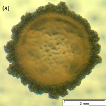
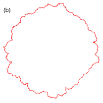
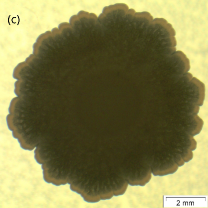
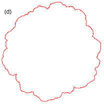
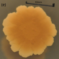
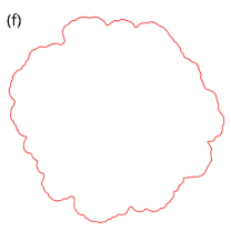
Figure 1: Experimental photographs of the bacterial colonies (left column, (a, c, e)) and profiles extracted using the procedure described in the text (right column, (b, d, f)). All these examples corresponds to B. subtilis with $C_{n}=20$ g/l. The growth times are: (a, b) 19 h, (c, d) 168 h, and (e, f) 792 h, top to bottom.

II.1 Extraction of front profiles

We next consider the protocol that we have followed in order to extract the position of the fronts of the bacterial colonies from the photographs. The analysis was semi-automatic. An algorithm was developed, which works in the majority of the cases without supervision. The images were digitized and subject to a constrast filter in order to highlight the interface. The resulting image can be regarded as a matrix with entries equal to $1$ inside the colony and equal to $0$ outside the colony. Then, a discretized continuous curve was obtained as follows. First, the geometric center of the colony bulk was estimated. Then we obtained the intensity curve along rays emanating from that point for different angles, $I_{\theta}(r)$. For each angle $\theta$, we obtained the distance $r(\theta)$ from the center, such that a certain threshold value of the total intensity was found below it. Mathematically,

$$\int_{0}^{r(\theta)}dr\,I_{\theta}(r)=\mu\int_{0}^{\infty}dr\,I_{\theta}(r),$$ (1)

where $\mu$ is the threshold parameter. In our present case, $\mu=0.99$ was employed, i.e., the radius $r(\theta)$ is defined as the first percentile of the intensity distribution. As an illustration, Fig. 1 shows a set of experimental photographs and their corresponding profiles. Note the compact form of the bacterial colony, delimited by a well-defined front that fluctuates around an average circular shape.

III Effective model

The evolution of the colony front can be rationalized through a kinetic continuum model for the dynamics of the front position. In this model the detailed dynamics of relevant physical fields (e.g., bacterial and nutrient densities) other than the position, $\vec{r}(t)$, of the front itself, is neglected. The model is tailored so as to capture purely the form and the dynamics of the front, in a similar way to many other instances of diffusion-limited growth, like thin solid films Bales et al. (1990); Ojeda et al. (2000); Castro et al. (2012) or combustion fronts Frankel and Sivashinsky (1995); Blinnikov and Sasorov (1996), in which this type of approach has proven useful. Specifically, we consider

$$\partial_{t}\vec{r}=\left(A_{0}+A_{1}K(\vec{r})+A_{a}\Theta_{a}(\vec{r})+A_{n}\eta\right)\vec{n},$$ (2)

where $\vec{r}$ is an interface point, $\vec{n}$ is the local exterior normal, $K(\vec{r})$ denotes the curvature of the interface at that point, $\Theta_{a}(\vec{r})$ is the local aperture angle and $\eta$ is a zero-average Gaussian uncorrelated space-time noise. Furthermore, $A_{0}$, $A_{1}$, $A_{a}$ and $A_{n}$ are parameters which quantify, respectively, the relative strengths of the average growth velocity of a planar front, surface tension, the dependence on the aperture angle, and fluctuations. Equation (2) is similar to continuum models earlier put forward in the context of growth of thin solid films limited by diffusive transport, see e.g. Meakin (1998). Note that, in contrast with many works in that field, Eq. (2) applies to interfaces with an arbitrary geometry, in particular with an average circular shape, and is not affected by small-slope, nor no-overhang approximations. In this sense, the model can be considered a stochastic generalization of a previous equation put forward in the context of combustion fronts Frankel and Sivashinsky (1995); Blinnikov and Sasorov (1996), for which transport also takes place by diffusion.

In our model, we assume that growth resources increase locally with the angle under which a given point $\vec{r}$ at the interface sees the exterior world, which we describe as the aperture angle, $\Theta_{a}(\vec{r})$, wich is illustrated by the sketch on Fig. 2 and further in Fig. 3. Intuitively, points inside cavities get less nutrient than those at local protuberances. As frequently done in the context of diffusion-limited growth, one may make an analogy Meakin (1998) to an ensemble of grass leaves which are striving to collect sunlight: taller leaves cast shadows on shorter ones, hindering growth of the latter. With this metaphor in mind, we consider this term to implement a shadowing effect, as frequently done in the context of DL growth Meakin (1998).

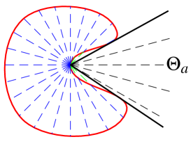
Figure 2: Given an interface (shown by the curved red solid line), and a point $\vec{r}$ on it, let us consider all the rays emanating from this point (dashed straight lines), and find out the fraction of rays that do not intersect the interface again (those delimited on the right side of the figure by the straight black solid lines). Such a fraction provides the local aperture angle, $\Theta_{a}(\vec{r})$.

Mathematically, the computation of the aperture angle is performed as follows. Let $\Gamma$ be the interface, with $\vec{r}_{0}$ and $\vec{r}$ being points on it. Let $A(\vec{r},\vec{r}_{0})$ be the angle under which $\vec{r}$ is seen from $\vec{r}_{0}$. Then, the aperture angle from point $\vec{r}_{0}$ is given by

$$\Theta_{a}(\vec{r}_{0})=2\pi-\left|\mbox{Range}_{\vec{r}\in\Gamma}\left(A(\vec{r},\vec{r}_{0})\right)\right|.$$ (3)

i.e. the measure of the range of function $A(\vec{r},\vec{r}_{0})$ when $\vec{r}$ takes values on $\Gamma$.

Equation (2) implements the basic mechanisms influencing growth dynamics: on average, the front tends to minimize its length and grows along the local normal direction, faster at those locations $\vec{r}$ which are more exposed [larger aperture angle $\Theta_{a}(\vec{r})$] to the external diffusive fluxes; moreover, the front position experiences stochastic fluctuations related with microscopic events (nutrient transport and consumption, as well as cell division and relocation). The choice of these mechanisms is supported by more detailed continuum models of bacterial colonies Dockery and Klapper (2002); Giverso et al. (2015, 2016) which find the front to be unconditionally unstable to perturbations. In particular, no quenched disorder is assumed.

In order to simulate Eq. (2), we have proceeded along the lines of Rodríguez-Laguna et al. (2011); Santalla et al. (2014): the interface is discretized in an adaptive way, adding and removing points dynamically in order to keep a constant spatial resolution. The normal vector and the local curvature are computed using concepts from discrete geometry. An important element of the simulation is that the interface is always a simple curve, although it can have overhangs: self-intersections are removed.

The evaluation of the aperture angle is the most costly part of the calculation to simulate Eq. (2), since it is a global measurement. We have devised the following algorithm in order to compute it. Given a point $P$ and a segment $P_{1}P_{2}$, we define the minimal angle-interval as the counterclockwise ordered pair $\alpha(P,P_{1}P_{2})\equiv(\alpha_{0},\alpha_{1})$ of angles, with respect to the horizontal, under which the segment is viewed from the point. If a segment is extended to a chain $P_{1}\cdots P_{n}$, we just compute the union of all angle-intervals. The aperture angle is the complementary of the measure of the final angle-interval.

In order to assess the type of morphological instability implied by the aperture term in Eq. (2), we have simulated it numerically by setting to zero all other terms in the equation. We have performed a linear stability analysis of the ensuing model by studying the rate of growth or decay in time for sinusoid-like perturbations of an overall circular shape (not shown). We have verified the expected unstable behavior: the amplitude of a small perturbation grows with a velocity proportional to the wave-number $k$ of the perturbation. In the case of a band geometry with periodic boundary conditions, this means that, according to Eq. (2),

$$\partial_{t}h_{k}(t)\simeq|k|\,h_{k}(t)+\cdots,$$ (4)

where $h_{k}(t)$ is the amplitude of a small sinusoidal perturbation of a flat profile with wave-vector $k$. This is indeed the well-known behavior of the aperture-angle term, as elucidated in other diffusion-limited systems Meakin (1998); Frankel and Sivashinsky (1995); Blinnikov and Sasorov (1996). The growth law Eq. (4) corresponds specifically to the destabilizing component of the classic Mullins-Sekerka instability, paradigmatic of diffusion-limited growth Vicsek (1992); Meakin (1998).

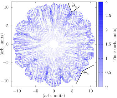
Figure 3: Interfaces from numerical simulations of Eq. (2) for $A_{0}=0$, $A_{1}=0.1$, $A_{a}=1$, $A_{n}=0.1$ and a circular initial condition. Sketches further illustrate the meaning of the local aperture angle $\Theta_{a}(\vec{r})$. The growth time for each profile can be read from the color bar on the right. Space and time units are arbitrary.

Figure 3 shows the time evolution of an initially circular interface described by Eq. (2), as obtained from numerical simulations for a representative choice of parameters. Once the interface perimeter grows large enough, the shadowing instability indeed sets in, reflecting the preferential growth at front protrusions, as compared with front troughs. In strong similarity with the experimental profile on the Fig. 1, the colony remains a compact aggregate for all $t$, with a front that fluctuates around an average circular shape.

IV Experimental Results

In this section we report our experimental results for BS and EC conlonies. Along with the various experimental properties studied, we additionally consider numerical simulations of Eq. (2) as aids to interpret the experimental results.

IV.1 Time evolution: Radius and global roughness

We first consider quantitatively the time evolution of our experimental BS and EC colonies through the average radius and global roughness of the colony fronts: After front extraction as described in Sec. II, each profile is a set of $N$ points on the plane, $\{x_{i},y_{i}\}_{i=1}^{N}$. This set is employed to obtain the radius, $R$, of the best fitting circle, using a minimization procedure to find the corresponding center $(x_{\rm C},y_{\rm C})$. The deviations from the fitting circle provide the global roughness or surface width,

$$W\equiv{\left<\frac{1}{N}\sum_{i=1}^{N}\left(\sqrt{(x_{i}-x_{\rm C})^{2}+(y_{i}-y_{\rm C})^{2}}-R\right)^{2}\right>}^{1/2},$$ (5)

where brackets denote averages over experimental realizations.

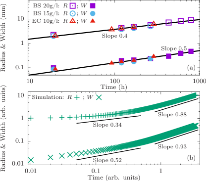
Figure 4: (a) Experimental radius $R$ (open symbols) and roughness $W$ (solid symbols) vs growth time. Purple and blue (red) symbols are for BS (EC), with $C_{n}$ as in the legend. Lines are fits to power laws, $R\sim t^{n}$ and $W\sim t^{\beta}$, with $n\approx 0.4$ and $\beta\approx 0.5$. (b) $+$ ($\times$) symbols are data for $R$ ($W$) from numerical simulations of Eq. (2) for parameters as in Fig. 3, averaged over 500 noise realizations. The lines represent power-laws $R\sim t^{n}$ and $W\sim t^{\beta}$ with different values of $n$ and $\beta$ for short and long times, as indicated. Units are arbitrary.

Both the radius and the global roughness of the experimental colony fronts depend on growth time. Results for $R(t)$ and $W(t)$ are provided in the top panel of Fig. 4. Data can be fit by power laws in both cases, $R(t)\sim t^{n}$ and $W(t)\sim t^{\beta}$, with $n\simeq 0.38$–$0.43$ and $\beta\simeq 0.47$–$0.52$ values which are similar for different nutrient concentration values and bacterial species. Usually, for experimental circular interfaces that display Eden/KPZ fluctuations Takeuchi and Sano (2010); Yunker et al. (2013a) —conspicuously including (Vero) cell aggregates Huergo et al. (2011)—, the average front velocity is constant, hence the average front position increases linearly with time. At variance with this, the radial growth rate we measure is sublinear, i.e., $n<1$. On the other hand, $W$ follows power-law behavior with time as in standard kinetic roughening systems. Taking into account that uncorrelated surface growth (so-called random deposition, RD) is characterized by $\beta_{\rm RD}=0.5$ Barabási and Stanley (1995), our relatively large experimental $\beta$ values are suggestive of uncorrelated, or possibly unstable growth wherein front fluctuations are amplified and grow even faster than in mere RD Vicsek (1992); Barabási and Stanley (1995); Meakin (1998). As noted in Bonachela et al. (2011), to date no other experimental work on bacterial colony growth provides information on the time evolution of $R(t)$ or $W(t)$ under our working conditions, in spite of the fact that universality classes are defined by two independent exponents Vicsek (1992); Barabási and Stanley (1995); Meakin (1998), one of them related with time-dependent behavior.

For the sake of comparison, the bottom panel of Fig. 4 shows the average radius and global roughness obtained from numerical simulations of our model, Eq. (2). Apparently in contrast with the experiment, for each magnitude two different regimes can be distinguished, one for short times and a different one for long times, within which the power laws are characterized by different exponent values. Note that the numerical values of the exponents which are closest to those of the experiments correspond to the model short-time regime. Actually, taking e.g. BS colonies with $C_{n}=20$ g/l as a representative case, we can make a more detailed comparison between the experimental behavior of $W(t)$ and $R(t)$ with that predicted by Eq. (2).

IV.1.1 Simulations in physical units

The experimental data for the evolution of the global roughness agree closely with the early time behavior of the simulations; these were performed for several sets of parameter values, with very similar results. The specific choice given in Fig. 3 (namely, $A_{0}=0$, $A_{1}=0.1$, $A_{a}=1$ and $A_{n}=0.1$) turned out to be the most relevant one to our experimental system. Of course, the units for these constants are arbitrary in principle. However, we can convert them into physical units through detailed comparison with the experimental data, as follows.

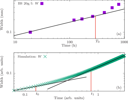
Figure 5: (a) Magnified view of the global roughness of a BS bacterial colony studied in Fig. 4. The time marked as $T_{0}$ indicates a change in the power-law behavior. (b) Magnified view of the roughness from numerical simulations of Eq. (2) using parameters as in Fig. 4. Time $t_{0}$ corresponds to the initial change in scaling behavior. Time $t_{1}$, signalling the beginning of asymptotic, long-time behavior, is also indicated.

In Fig. 5(a) we show the roughness of the interface, $W(t)$, for the same B. subtilis experiments with $C_{n}=20$ g/l considered in Fig. 4, but in a magnified view. A certain time $T_{0}=297$ hour (h) can be identified which marks a change in the power-law behavior of the data, at which the global roughness is $W_{0}=0.25$ mm. The experiment ends at time $T_{e}=801$ h, when $W_{e}=0.47$ mm. Thus, we have $W_{e}/W_{0}=1.9$ and $T_{e}/T_{0}=2.7$. The physical occurrence of $T_{0}$ can be confirmed by in other measurable quantitites, such as the average front velocity, see Fig. 6.

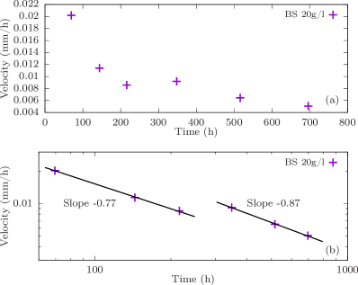
Figure 6: Average front speed as a function of time for BS experiments using $C_{n}=20$ g/l in linear (a) and doubly-logarithmic (b) displays. The data group themselves into two scaling regimes, approximately separated at $T_{0}=297$ h.

The front speed is estimated by comparing consecutive measurements of the radius and using a finite-differences approach. The two panels show the same data, the only difference between them being that the bottom one is shown in logarithmic scale. We can see how the data divide into two sequences of points with slightly different scaling behavior, with the division approximately corresponding to $T_{0}=297$ h.

Coming back to the simulations of Eq. (2), Fig. 5(b) indicates a change in the scaling behavior of the global roughness at time $t_{0}=0.14$ [T], with a roughness of $w_{0}=0.044$ [L], where [L] and [T] are length and time units, respectively. Thus, the end of the experiment should correspond to a roughness $w_{e}=0.044$ [L] $\times 1.9=0.084$ [L], which takes place at $t_{e}\sim 0.44$ [T]. We make this time correspond to $T_{e}=801$ h. Thus, the numerical conversion from arbitrary time units to hours is $801$ h$/0.44$ [T] $\approx 1800$ h/[T]. The same reasoning can be performed with the length unit and we obtain a conversion factor of $0.47$ mm$/0.044$ [L] $\approx 11$ mm/[L]. Alternative procedures can be designed to obtain the conversion factors, and they all provide similar results. At any rate, using the indicated conversion factors we can estimate the physical values of the equation parameters in physical units, namely, $A_{0}=0$ mm/h, $A_{1}=0.067$ mm²/h, $A_{a}=6.1\cdot 10^{-3}$ mm/h, $A_{n}=0.086$ mm^3/2/h^1/2. Experimental data are compared with simulations for this parameter choice in Fig. 7.

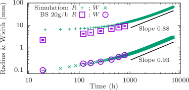
Figure 7: Evolution of the radius and global roughness predicted by Eq. (2) with physical parameters $A_{0}=0$ mm/h, $A_{1}=0.067$ mm²/h, $A_{a}=6.1\cdot 10^{-3}$ mm/h, $A_{n}=0.086$ mm^3/2/h^1/2. Squares (circles) are experimental radius (roughness) for BS with $C_{n}=20$ g/l; error bars are of the same size as symbols or smaller, see appendix A.

With respect to $W(t)$, agreement is reached for essentially the full duration of the experiments. For times longer than approximately $800$ hours (which remain beyond our experimental setup), Eq. (2) predicts almost linear increase with time for $W(t)$ and $R(t)$. The agreement between experimental and simulation data is slightly worse in the case of $R(t)$, for which the initial condition plays a stronger role in the continuum model. Nevertheless, agreement also becomes quantitative for $t>100$ hours. Note, the time $t_{1}$ required for the onset of long-time, asymptotic behavior in the experiments can be assessed from the numerical simulation of Eq. (2), see the bottom panel of Fig. 5. We estimate $t_{1}=0.8$, which approximately corresponds to $1440$ hours. Overall, Fig. 7 suggests that the scaling behavior reached in the experiments is preasymptotic, clear-cut asymptotics occurring for $t>t_{1}$, approximately twice our longest experimental growth time.

IV.2 Geometrical properties: Local roughness and radial correlations

Further non-trivial properties of the experimental colonies involve the spaial dependence of front fluctuations. We can characterize them quantitatively by considering the so-called local roughness, $w(\ell)$, which evaluates interface deviations from an average position, within observation windows of size $\ell$ Vicsek (1992); Barabási and Stanley (1995); Meakin (1998). We proceed as is customary for systems with an overall circular symmetry Meakin (1998); Santalla et al. (2014): Namely, each point on the front is converted to polar coordinates emanating from the geometric center, $(x_{i},y_{i})\to(\theta_{i},r_{i})$, whereby $\theta_{i}$ ($r_{i}$) is considered a new independent (dependent) variable. Given an initial point $\vec{r}_{0}$ and a length scale $\ell$, we consider the set of points within a circle centered at $\vec{r}_{0}$ with radius $\ell$. Then, we make a fit to the straight line which minimizes the deviations. The mean-square distance of the front positions to that fitting line provides the local roughness $w(\ell)$. Results for our experimental BS and EC colonies are displayed in Fig. 8.

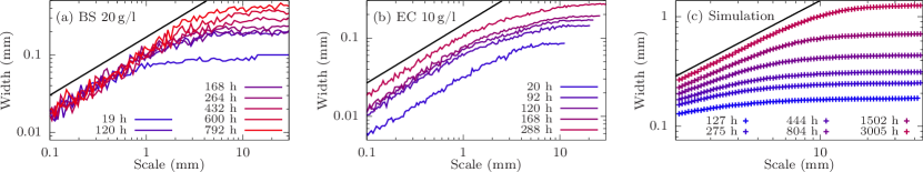
Figure 8: Experimental length-scale dependence of the local roughness of BS (a) and EC (b) colony fronts for different times and $C_{n}$ as indicated in the legends. (c) Same observable for numerical simulations of Eq. (2) as in Fig. 3. All straight lines represent $w(\ell)\sim\ell^{0.75}$.

An approximate power-law dependence, $w(\ell)\sim\ell^{\alpha}$, holds at intermediate scales above 100 $\mu$m, and up to $3$ mm for the most favorable cases, with $\alpha\simeq 0.75$. For the sake of comparison, we recall that a one-dimensional interface provided by the world-line of an uncorrelated random walk features $\alpha_{\rm RW}=1/2$ Vicsek (1992); Barabási and Stanley (1995); Meakin (1998). Our experimental value for $\alpha$ is in the same range as those found earlier for similar bacterial colony experiments Vicsek et al. (1990); Wakita et al. (1997); Bonachela et al. (2011) and is also similar to values measured in other DL systems, like 1D ECD Pastor and Rubio (1996); Huo and Schwarzacher (2001) or 2D thin films grown by CVD under low sticking conditions Ojeda et al. (2000); Zhao et al. (2000). In these contexts, such large $\alpha$ are known not to correspond to any well-defined universality class of kinetic roughening Castro et al. (2000); Nicoli et al. (2009a); Castro et al. (2012), but to merely reflect the large surface slopes that ensue, due to diffusive instabilities. Such instabilities are actually well-known to correlate with front branching Vicsek (1992); Barabási and Stanley (1995); Meakin (1998), which in our experiments can be assessed through the behavior of the autocorrelation of the radial interface fluctuations as a function of the angular distance,

$$C(\Delta\theta,t)=\langle[r(\theta,t)-R(t)][r(\theta+\Delta\theta,t)-R(t)]\rangle.$$ (6)

As seen in Fig. 9, and in spite of the compactness of the colonies, $C(\Delta\theta,t)$ vanishes approximately at the same angular distance for different times, indicating fronts that develop well-defined branches. Moreover, the importance of such branching increases monotonically along the experimental time evolution. Such a behavior is analogous to the result of detailed continuum models of bacterial colony growth put forward in Giverso et al. (2015, 2016), which predict unconditional instability of the colony front to perturbations for a variety of relaxation mechanisms that include both, chemotactic and volumetric expansions. In application of the analysis in Giverso et al. (2015, 2016) to our data, Fig. 10 shows the time evolution of the area/perimeter ratio for the experimental colonies, compared to the $R(t)/2$ value that would correspond to a perfectly circular front in each case; clearly the actual perimeter grows too fast with time relative to the enclosed area, as compared with expectations for an ideally circular front. Such a behavior is inconsistent in particular with the occurrence of Eden behavior at long times Vicsek (1992); Barabási and Stanley (1995); Meakin (1998).

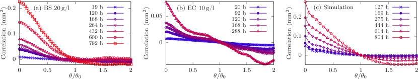
Figure 9: Left to right: Autocorrelation function of experimental radial fluctuations vs angular distance rescaled by $\theta_{0}$, for BS (a), EC (b), and simulations (c) of Eq. (2) with parameters as in Fig. 3, where $\theta_{0}=30^{\circ},60^{\circ}$, and $15^{\circ}$, respectively. Times and $C_{n}$ are as given in the legends.

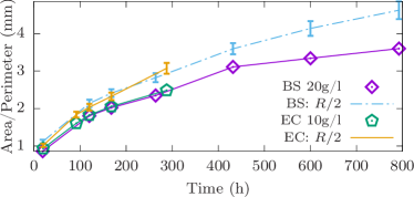
Figure 10: Experimental area/perimeter ratio vs time. Symbols are direct measurements for conditions described in the legend; lines show $R(t)/2$ as obtained from Fig. 4 for the corresponding sets of data.

The geometrical properties of the front observed in the experiments are very similarly found also in the simulations of Eq. (2). Figure 8 shows the dependence of the simulated local roughness with length scale for different times, readily compared with the experimental data in the same figure. Indeed, for small scales the model yields $w(\ell)\sim\ell^{\alpha}$, with $\alpha$ increasing with time up to 0.75, very close to the experimental value. Comparison between the model and the experiments improves with increasing times, as typical length-scales also increase. Note, these simulation data include the long-time, asymptotic regime identified for the model in Fig. 4. Finally, the behavior in simulations of the radial autocorrelation function $C(\Delta\theta,t)$ also supports our interpretation on branching at the interface: Figure 9 indeed shows the selection of a precise correlation angle value $\theta_{0}$, analogous to the experimental morphologies.

V Discussion and Conclusions

Summarizing our experimental observations for both BS and EC colonies in the suppressed-motility conditions Wakita et al. (1997); Matsushita et al. (1998); Ràfols (1998) which are in the classically alleged Eden regime, we obtain branched interfaces with scaling exponents $\beta\simeq 0.5$ and $\alpha\simeq 0.75$, which unambiguously differ from Eden/KPZ behavior, characterized by non-branched interfaces, $\beta_{\rm KPZ}=1/3$, and $\alpha_{\rm KPZ}=1/2$ Vicsek (1992); Barabási and Stanley (1995); Meakin (1998). Our experimental data are also inconsistent with quenched noise effects which, e.g., allegedly induce $\beta=0.61,\alpha=0.68$ in agent-based simulations of bacterial colonies Bonachela et al. (2011), or with the so-called quenched KPZ (qKPZ) equation Barabási and Stanley (1995). Unconditioned by any comparison to models, the fact that our experimental colony profiles become increasingly branched during all accessible times (Figs. 9 and 10) moreover suggests that the observed scaling is preasymptotic behavior for a system whose asymptotics is not Eden, and we speculate that this could also be the case for other, classical, experiments Vicsek et al. (1990); Wakita et al. (1997) performed under conditions which are similar to ours.

Given the semi-quantitative agreement between our experiments and simulations of the effective model, Eq. (2), we can consider the latter in order to predict what would be the actual asymptotic behavior of the former. Indeed, Eq. (2) predicts a long-time behavior with $\beta=0.93$ (Fig. 4) and $\alpha=0.75$ (Fig. 8). Actually, a small-slope approximation of Eq. (2) yields dimension-independent exponents $\alpha=\beta=1$ Nicoli et al. (2009a, b) —recently measured in CVD under DL conditions Castro et al. (2012)—, which are definitely non-KPZ and are expected to characterize Eq. (2) at long times. Note, for interfaces with $\alpha\gtrsim 1$, local measurements using $w(\ell)$ are known to underestimate the correct value of the roughness exponent Castro et al. (2000), explaining our $\alpha=0.75$ value. Parameter conditions in our experiments would make such a long-time regime hardly accessible, requiring growth times at least twice the longest time that we have been able to reach, as estimated in Sec. IV.1.1. On the other hand, the preasymptotic ($t<800$ h) behavior in Eq. (2) —during which $W(t)$ evolves as in our experiments— is dominated by the diffusive (shadowing) instabilities that induce branching of the front and large exponent values. In such a case, and as shown for other DL systems Nicoli et al. (2009a); Castro et al. (2000, 2012), the exponent values are non-universal and may depend on parameter values and even on the specific space/time ranges in which power-law fits are attempted.

In conclusion, bacterial colonies where individual motility is suppressed form compact aggregates whose front morphology can still be dominated by diffusive instabilities. For our experimental conditions, similar to those in Wakita et al. (1997); Matsushita et al. (1998); Ràfols (1998), preasymptotic scaling seems to occur at the accessed times, which in any case is not in the Eden/KPZ universality class. There is no need to invoke quenched disorder to account for this discrepancy. Rather, the shadowing instability induces large front fluctuations with non-universal scaling. This behavior is strongly reminiscent of many other experimental systems Pastor and Rubio (1996); Ojeda et al. (2000); Zhao et al. (2000); Huo and Schwarzacher (2001); Yunker et al. (2013a) in which transport-induced instabilities induce effective scaling. In some of these cases Yunker et al. (2013a) the observed kinetic roughening properties have also been associated with the qKPZ universality class, due to accidental similarities in the values of the scaling exponents Nicoli et al. (2013); Yunker et al. (2013b); Oliveira and Aarão Reis (2014). Note, attributing a set of scaling exponents to a well-defined, asymptotic, universality class like qKPZ, or to non-universal preasymptotic behavior as we are presently advocating for, are conceptually very different interpretations.

Non-KPZ exponents due to diffusive instabilities are also predicted by agent-based simulations Farrell et al. (2013, 2017) for small values of the active layer thickness $\delta$. However, for sufficiently large $\delta$ very compact colonies with extremely flat fronts are found Farrell et al. (2013, 2017). While this seemingly questions the prevalence of diffusive instabilities, continuum models Giverso et al. (2015, 2016) analytically predict such flat front conditions to be a finite-size effect. Thus, parameter conditions select a typical length-scale $\ell_{0}$ for the instabilities, which is well defined for any value of $\delta$. As standard in pattern formation Cross and Greenside (2009), the correlation length along the front (initially a few cell sizes across) needs to increase up to $\ell_{0}$ for the instability to set in. If $\ell_{0}$ is very large (in band geometry, for systems smaller than $\ell_{0}$), the front may effectively be flat. In circular geometries, for sufficiently (perhaps, exceedingly) long times, the instability will still occur.

We should still note that additional systems exist, which are closely related to the ones we study, and for which Eden/KPZ scaling does occur. For instance, bacterial colonies for which individual motility is non-negligible Wakita et al. (1997) yield a roughness exponent compatible with the 1D KPZ value. Also, aggregates of non-cancerous (Vero) or cancerous (HeLa) primate cells display unambiguous KPZ Huergo et al. (2011), and even qKPZ Huergo et al. (2014); Muzzio et al. (2016), scaling, as is the case with fungal growth López and Jensen (2002). Experimentally, KPZ scaling also applies to fluctuating frontiers between different genetic strains in range expansion of E. coli Hallatschek et al. (2007), although deviations from Eden behavior can also occur Kuhr et al. (2011); Reiter et al. (2014). In general, individual cell motility seems to play a relevant role, to the extent that instabilities associated with nutrient transport can eventually be superseded. Indeed, the Eden model Eden (1961) will at any rate stand as the prime example for reaction-limited growth Vicsek (1992); Barabási and Stanley (1995); Meakin (1998), where nutrient transport is, effectively, infinitely fast and irrelevant to front fluctuations.

Appendix A Some error estimates

For each bacterial species and nutrient concentration we have only one sample available. Therefore, the error bars on the measurements of the radius and the roughness can not be estimated via statistical error between different samples. An alternative approach is to consider that measurements performed on different parts of the interface constitute a suitable statistical ensemble from which we can estimate the magnitude of the desired fluctuations. Thus, the global roughness itself provides an estimate for the uncertainty in the measurement of the radius.

The estimate of the fluctuations of the roughness is more involved. Our approach is to divide the interface into patches of size $\ell$ and measure the estimate for each of them, $W_{i}(\ell)$. Then, for each size $\ell$ we can determine the deviation of those measures,

$$\sigma^{2}_{W}(\ell)=\left\langle W^{2}(\ell)\right\rangle-\left\langle W(\ell)\right\rangle^{2}.$$ (7)

Naturally, this deviation will depend on the measurement scale $\ell$. We have thus chosen the worst case to determine our estimate for the error in the roughness, namely,

$$\sigma^{2}_{W}=\max_{\ell}\sigma^{2}_{W}(\ell).$$ (8)

This is how the error bars are estimated in Fig. 7. The behavior of $\sigma_{W}(\ell)$ for the fronts of BS colonies grown with $C_{n}=20$ g/l is shown as an illustration in Fig. 11.

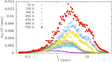
Figure 11: Scale dependence of the estimate for the error in the global roughness obtained using Eq. (7), when applied to the profiles of our BS sample grown with $C_{n}=20$ g/l. The actual estimate is provided by the maximum of each curve.

References

- Ramaswamy (2010) S. Ramaswamy, Ann. Rev. Condens. Matter Phys 1, 323 (2010).
- Marchetti et al. (2013) M. C. Marchetti, J. F. Joanny, S. Ramaswamy, T. B. Liverpool, J. Prost, M. Rao, and R. A. Simha, Rev. Mod. Phys. 85, 1143 (2013).
- Ben-Jacob et al. (2000) E. Ben-Jacob, I. Cohen, and H. Levine, Adv. Phys. 49, 395 (2000).
- Sokolov et al. (2007) A. Sokolov, I. S. Aranson, J. O. Kessler, and R. E. Goldstein, Phys. Rev. Lett. 98, 158102 (2007).
- Zhang et al. (2010) H. P. Zhang, A. Be’er, E.-L. Florin, and H. L. Swinney, Proc. Natl. Acad. U.S.A. 107, 13626 (2010).
- Ben-Jacob et al. (1998) E. Ben-Jacob, I. Cohen, and D. L. Gutnick, Ann. Rev. Microbiol. 52, 779 (1998).
- Matsushita et al. (2004) M. Matsushita, F. Hiramatsu, N. Kobayashi, T. Ozawa, Y. Yamazaki, and T. Matsuyama, Biofilms 1, 305 (2004).
- Bonachela et al. (2011) J. A. Bonachela, C. D. Nadell, J. B. Xavier, and S. A. Levin, J. Stat. Phys. 144, 303 (2011).
- Vicsek (1992) T. Vicsek, Fractal growth phenomena (World Scientific, Singapore, 1992).
- Barabási and Stanley (1995) A.-L. Barabási and H. E. Stanley, Fractal concepts in surface growth (Cambridge University Press, New York, 1995).
- Meakin (1998) P. Meakin, Fractals, scaling and growth far from equilibrium (Cambridge University Press, Cambridge, UK, 1998).
- Fujikawa and Matsushita (1989) H. Fujikawa and M. Matsushita, J. Phys. Soc. Jpn. 58, 3875 (1989).
- Vicsek et al. (1990) T. Vicsek, M. Cserzö, and V. K. Horváth, Physica A 167, 315 (1990).
- Wakita et al. (1997) J. I. Wakita, H. Itoh, T. Matsuyama, and M. Matsushita, J. Phys. Soc. Jpn. 66, 67 (1997).
- Matsushita et al. (1998) M. Matsushita, J. Wakita, H. Itoh, I. Ràfols, T. Matsuyama, H. Sakaguchi, and M. Mimura, Physica A 249, 517 (1998).
- Nicoli et al. (2009a) M. Nicoli, M. Castro, and R. Cuerno, J. Stat. Mech.: Theor. Exp. , P02036 (2009a).
- Nadell et al. (2010) C. D. Nadell, K. R. Foster, and J. B. Xavier, PLoS Comp. Biol. 6, e1000716 (2010).
- Mitri et al. (2011) S. Mitri, J. B. Xavier, and K. R. Foster, Proc. Natl. Acad. U.S.A. 108, 10839 (2011).
- Nadell et al. (2013) C. D. Nadell, V. Bucci, K. Drescher, S. A. Levin, B. L. Bassler, and J. B. Xavier, Proc. Roy. Soc. B 280, 20122770 (2013).
- Costerton et al. (1995) J. W. Costerton, Z. Lewandowski, D. E. Caldwell, D. R. Korber, and H. M. Lappin-Scott, Ann. Rev. Microbiol. 49, 711 (1995).
- Wilking et al. (2011) J. N. Wilking, T. E. Angelini, A. Seminara, M. P. Brenner, and D. A. Weitz, MRS Bulletin 36, 385 (2011).
- Eden (1961) M. Eden, in Proceedings of the 4th. Berkeley Symposium on Mathematical Statistics and Probability, Vol. 4, edited by J. Neyman (U. California Press, Berkeley, 1961) pp. 223–239.
- Kardar et al. (1986) M. Kardar, G. Parisi, and Y.-C. Zhang, Phys. Rev. Lett. 56, 889 (1986).
- Alves et al. (2011) S. G. Alves, T. J. Oliveira, and S. C. Ferreira, EPL 96, 48003 (2011).
- Takeuchi (2012) K. A. Takeuchi, J. Stat. Mech.: Theor. Exp. , P05007 (2012).
- Halpin-Healy and Takeuchi (2015) T. Halpin-Healy and K. A. Takeuchi, J. Stat. Phys. 160, 794 (2015).
- Van Beijeren (2012) H. Van Beijeren, Phys. Rev. Lett. 108, 180601 (2012).
- Mendl and Spohn (2013) C. B. Mendl and H. Spohn, Phys. Rev. Lett. 111, 230601 (2013).
- Kulkarni and Lamacraft (2013) M. Kulkarni and A. Lamacraft, Phys. Rev. A 88, 021603(R) (2013).
- Nesic et al. (2014) S. Nesic, R. Cuerno, and E. Moro, Phys. Rev. Lett. 113, 180602 (2014).
- Lacasta et al. (1999) M. Lacasta, I. R. Cantalapiedra, C. E. Auguet, A. Peñaranda, and L. Ramírez-Piscina, Phys. Rev. E 59, 7036 (1999).
- Mimura et al. (2000) M. Mimura, H. Sakaguchi, and M. Matsushita, Physica A 282, 283 (2000).
- Dockery and Klapper (2002) J. Dockery and I. Klapper, SIAM J. Appl. Math. 62, 853 (2002).
- Kobayashi et al. (2004) N. Kobayashi, O. Moriyama, S. Kitsunezaki, Y. Yamazaki, and M. Matsushita, J. Phys. Soc. Jpn. 73, 2112 (2004).
- Giverso et al. (2015) C. Giverso, M. Verani, and P. Ciarletta, J. Roy. Soc. Interface 12, 20141290 (2015).
- Giverso et al. (2016) C. Giverso, M. Verani, and P. Ciarletta, Biomech. Model. Mechanobiol. 15, 643 (2016).
- Farrell et al. (2013) F. D. C. Farrell, O. Hallatschek, D. Marenduzzo, and B. Waclaw, Phys. Rev. Lett. 111, 168101 (2013).
- Farrell et al. (2017) F. D. Farrell, M. Gralka, O. Hallatschek, and B. Waclaw, J. Roy. Soc. Interface 14, 20170073 (2017).
- Ràfols (1998) I. Ràfols, Formation of concentric rings in bacterial colonies, Master’s thesis, Chuo University (1998).
- Castro et al. (2000) M. Castro, R. Cuerno, A. Sánchez, and F. Domínguez-Adame, Phys. Rev. E 62, 161 (2000).
- Yunker et al. (2013a) P. J. Yunker, M. A. Lohr, T. Still, A. Borodin, D. J. Durian, and A. G. Yodh, Phys. Rev. Lett. 110, 035501 (2013a).
- Nicoli et al. (2013) M. Nicoli, R. Cuerno, and M. Castro, Phys. Rev. Lett. 111, 209601 (2013).
- Yunker et al. (2013b) P. J. Yunker, M. A. Lohr, T. Still, A. Borodin, D. J. Durian, and A. G. Yodh, Phys. Rev. Lett. 111, 209602 (2013b).
- Oliveira and Aarão Reis (2014) T. J. Oliveira and F. D. A. Aarão Reis, J. Stat. Mech.: Theory Exp. , P09006 (2014).
- Bales et al. (1990) G. S. Bales, R. Bruinsma, E. A. Eklund, R. P. U. Karunasiri, J. Rudnick, and A. Zangwill, Science 249, 264 (1990).
- Ojeda et al. (2000) F. Ojeda, R. Cuerno, R. Salvarezza, and L. Vázquez, Phys. Rev. Lett. 84, 3125 (2000).
- Castro et al. (2012) M. Castro, R. Cuerno, M. Nicoli, L. Vázquez, and J. G. Buijnsters, New J. Phys. 14, 103039 (2012).
- Frankel and Sivashinsky (1995) M. L. Frankel and G. I. Sivashinsky, Phys. Rev. E 52, 6154 (1995).
- Blinnikov and Sasorov (1996) S. I. Blinnikov and P. V. Sasorov, Phys. Rev. E 53, 4827 (1996).
- Rodríguez-Laguna et al. (2011) J. Rodríguez-Laguna, S. N. Santalla, and R. Cuerno, J. Stat. Mech.: Theory Exp. , P05032 (2011).
- Santalla et al. (2014) S. N. Santalla, J. Rodríguez-Laguna, and R. Cuerno, Phys. Rev. E 89, 010401(R) (2014).
- Takeuchi and Sano (2010) K. A. Takeuchi and M. Sano, Phys. Rev. Lett. 104, 230601 (2010).
- Huergo et al. (2011) M. A. C. Huergo, M. Pasquale, P. González, A. Bolzán, and A. Arvia, Phys. Rev. E 84, 021917 (2011).
- Pastor and Rubio (1996) J. M. Pastor and M. A. Rubio, Phys. Rev. Lett. 76, 1848 (1996).
- Huo and Schwarzacher (2001) S. Huo and W. Schwarzacher, Phys. Rev. Lett. 86, 256 (2001).
- Zhao et al. (2000) Y. P. Zhao, J. B. Fortin, G. Bonvallet, G. C. Wang, and T. M. Lu, Phys. Rev. Lett. 85, 3229 (2000).
- Nicoli et al. (2009b) M. Nicoli, R. Cuerno, and M. Castro, Phys. Rev. Lett. 102, 256102 (2009b).
- Cross and Greenside (2009) M. Cross and H. Greenside, Pattern formation and dynamics in nonequilibrium systems (Cambridge University Press, 2009).
- Huergo et al. (2014) M. A. C. Huergo, N. E. Muzzio, M. A. Pasquale, P. H. P. González, A. E. Bolzán, and A. J. Arvia, Phys. Rev. E 90, 022706 (2014).
- Muzzio et al. (2016) N. E. Muzzio, M. A. Pasquale, M. A. C. Huergo, A. E. Bolzán, P. H. González, and A. J. Arvia, J. Biol. Phys. 42, 477 (2016).
- López and Jensen (2002) J. M. López and H. J. Jensen, Phys. Rev. E 65, 21903 (2002).
- Hallatschek et al. (2007) O. Hallatschek, P. Hersen, S. Ramanathan, and D. R. Nelson, Proc. Natl. Acad. U.S.A. 104, 19926 (2007).
- Kuhr et al. (2011) J. T. Kuhr, M. Leisner, and E. Frey, New J. Phys. 13, 113013 (2011).
- Reiter et al. (2014) M. Reiter, S. Rulands, and E. Frey, Phys. Rev. Lett.ç 112, 148103 (2014).