For this, we use two different experimental arrangements, which respectively use as the substrate an inclined plane or the inner surface of a slowly rotating hollow horizontal cylinder.

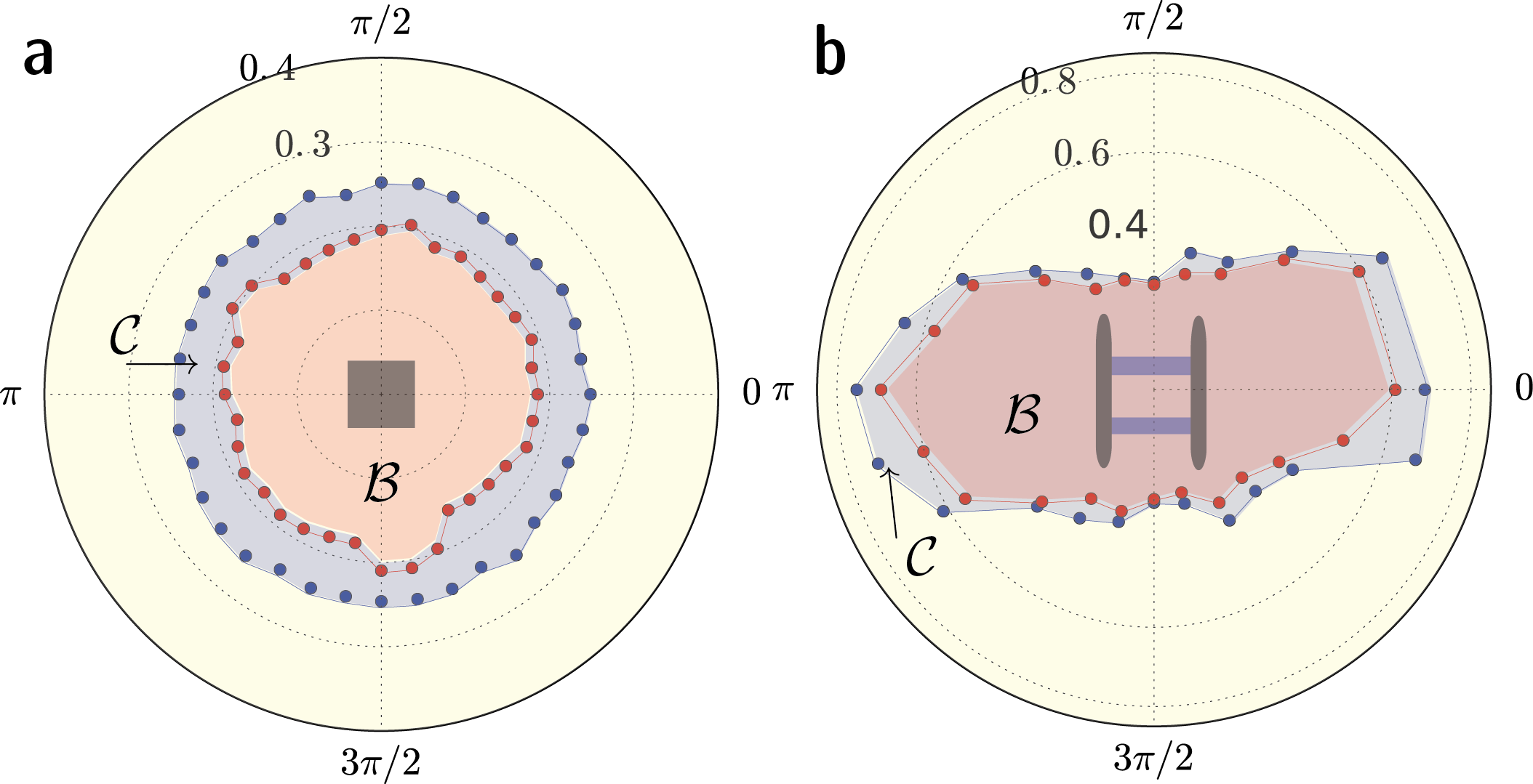
Figure 7: (a) The figure shows the empirically plotted regions $\mathcal{C}$ (blue) and $\mathcal{B}$ (red) of $\mathcal{A}(=\mathcal{B}\cup\mathcal{C})$ for a square plastic block (sides $=90\,\mbox{mm}$, height $=10\,\mbox{mm}$). In spite of the absence of circular symmetry in the block, the regions are approximately circular, showing that corner and edge effects are negligible in this case. (b) The figure shows the motion onset curve $\partial\mathcal{A}$ (blue),the subregion $\mathcal{C}$ (blue) and $\mathcal{B}$ (red) of $\mathcal{A}(=\mathcal{B}\cup\mathcal{C})$ for a sledge placed on a neoprene sheet. The sledge is made by gluing surgical blades to opposite sides of a square plastic block (length $=90\,\mbox{mm}$, height $=10\,\mbox{mm}$). In both these figures, the data points in blue are shown to be just inside the schematic plots of the corresponding regions, while the data points in red are just outside the region $\mathcal{B}$.

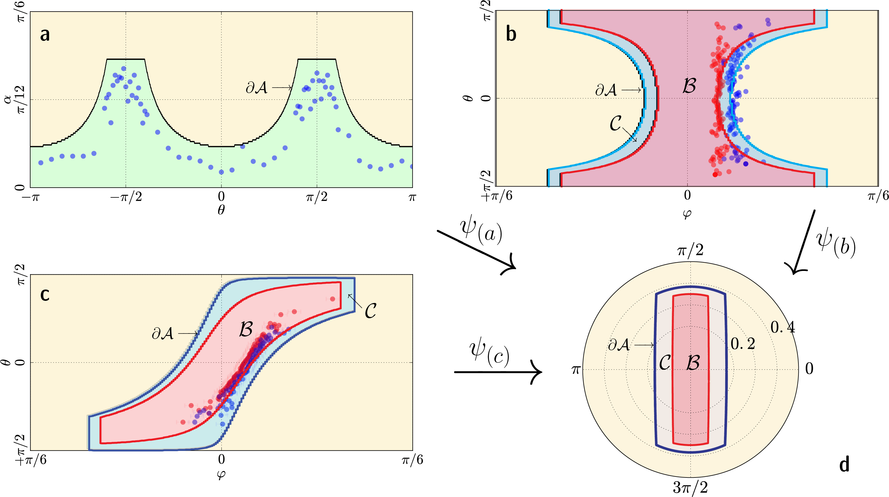
Figure 8: Classifying maps for frictional experiments with dumbbell: The panels (a), (b) and (c) show the plots for the onset curved for a dumbbell in terms of the control parameters for three different experimental arrangements. These onset curves are the pull backs under the respective classifying maps $\psi_{a}$, $\psi_{b}$ and $\psi_{c}$ of the universal onset curve in the phase space $E_{2}$ associated with a dumbbell on a glass substrate, shown in panel (d) with polar coordinates $(\bm{r},\bm{\theta})$. Inclined plane apparatus: The figure in panel (a) shows the region $\mathcal{A}$ plotted for a dumbbell placed on an inclined plane, in terms of the control parameters $\alpha$ and $\theta$. The map $\psi_{(a)}$ is given by $\bm{r}=\tan\alpha$ and $\bm{\theta}=\theta$. Horizontal cylinder apparatus: The figure in panel (b) shows the regions $\mathcal{A}$ and $\mathcal{B}$ plotted for a dumbbell placed on the inner surface of a horizontal cylinder apparatus, in terms of the control parameters $\varphi$ and $\theta$. The map $\psi_{(b)}$ is given by $\bm{r}=\tan\varphi$ and $\bm{\theta}=\theta$. Tilted cylinder apparatus: The figure in panel (c) shows the regions $\mathcal{A}$ and $\mathcal{B}$ plotted for a dumbbell placed on the inner surface of a tilted cylinder apparatus in terms of the control parameters $\varphi$ and $\theta$. The tilt of the cylinder from the horizontal is fixed at $\alpha=7^{\circ}$. The map $\psi_{(c)}$ is given by $\bm{r}=\sqrt{(\cos\alpha\sin\varphi)^{2}+\sin^{2}\alpha}/(\cos\alpha\cos\varphi)$ and $\bm{\theta}=\arccos\left((\sin\varphi\cos\theta-\tan\alpha\sin\theta)/(|\sqrt{\sin^{2}\varphi+\tan^{2}\alpha}|)\right)$. In (a), the plotted data points in blue are inside $\mathcal{A}$, while in (b) and (c), the blue points are inside $\mathcal{A}$ while the red points are inside $\mathcal{B}$. To plot $\mathcal{A}$ we used $\mu_{r}^{stat}=0.12$ and $\mu_{s}^{stat}=0.40$. Similarly, to plot $\mathcal{B}$ we used $\mu_{r}^{dyn}=0.08$ and $\mu_{s}^{dyn}=0.36$.

When the substrate is an inclined plane, the forces $F$ and $N$ are supplied by gravity, with $\lvert F\rvert/\lvert N\rvert=\tan\alpha$ where $\alpha$ is the inclination of the plane. We assume that we are in the realm of moderate $|N|$ even when the plane is horizontal so that $|N|$ is at its maximum. We note that $\alpha=0$ corresponds to a horizontal plane, and $\alpha=\pi/2$ corresponds to a vertical plane. Therefore, $\theta_{obj}$ is the angle between the chosen fiducial vector on the object and the downward direction on the inclined plane. We vary $\theta_{obj}$ by rotating the object around an axis perpendicular to the substrate. The height of the object is kept small compared to its lateral dimensions whenever we want the toppling torque produced by $F$ to be negligible. If one needs to test a non-isotropic substrate using this apparatus, this is possible by holding the angle $\theta_{sub}$ to be constant as $\alpha$ is slowly varied, and then repeating the experiment for a new value of $\theta_{sub}$. The angle of inclination $\alpha$ of the plane is mechanically increased slowly, at the rate of approximately $50$ degree per hour, starting with $\alpha=0$. For different chosen values of $\theta_{obj}$, note was made of the value of $\alpha$ at which the object began to move. This gave various data points with polar coordinates $(r,\theta)=(\tan\alpha,\,\theta_{obj})$ in $\mathcal{A}$, close to its boundary $\partial\mathcal{A}$ (the onset curve), which enabled a schematic plot of the region $\mathcal{A}$.

This arrangement is used to plot the region $\mathcal{A}$ in $E_{2}$ (with coordinates $(\lvert F\rvert/\lvert N\rvert,\theta_{obj})$ as described above), for different objects. If the object placed on the inclined plane is a circular disk and moreover the substrate is isotropic, it is clear by symmetry that the region $\mathcal{A}$ is the circular disk centred at the origin $r=0$ of $E_{2}$ with radius $\mu_{stat}$, and the onset curve $\partial\mathcal{A}$ is its boundary circle $r=\mu_{stat}$. If the object is not circular, there is no a priori reason for the onset curve to be a circle as above, and the actual shape of it must be measured experimentally.

The Figures LABEL:fig:sledge and 7 show the observations and the plotted onset curves for (1) a paper sledge on a grit paper, (2) a paper curled on one side on grit paper, (3) a plastic square block placed on a glass plate, (4) a sledge with metallic blades placed on a neoprene sheet and (5) a dumbbell placed on an glass plate. To minimize the toppling torque on the non-rolling objects (cases (1) to (4) above), their height was kept small compared to their lateral dimensions.

To plot the region $\mathcal{B}$, the plane was first kept inclined at various fixed values of the angle $\alpha$ at which the object remained stationary, and then a small burst of mechanical noise was imparted to the assembly, and its effect was observed. Note was made of whether the resulting motion of the object was transient or was a sustained movement. These observations approximately gave the boundary $\partial\mathcal{B}$ and so led to a schematic plot of region $\mathcal{B}$ (see Fig.   7). This experiment was done for a square block and a metal sledge. (The paper sledge and the plastic dumbbell, being too light, were not convenient for the administration of a mechanical burst, as they often got thrown off by the noise.)

The second experimental arrangement, namely, a rotating hollow horizontal cylinder, was used to plot the regions $\mathcal{A}$ and $\mathcal{B}$ and the onset curve $\partial\mathcal{A}$ for a dumbbell. In this experiment a hollow glass cylinder (radius$\,=125\mbox{mm}$) whose axis is horizontal is rotated very slowly around its axis (at an angular velocity $\approx 0.01\,\mbox{radians/sec}$). A dumbbell made of plastic (radius of the balls$\,=3\,\mbox{mm}$, length of the dumbbell$\,=23\,\mbox{mm}$) is placed at different angles (values of $\theta_{obj}$) at the lowermost point on the interior surface of the cylinder, and its subsequent motion is observed. As the radius of the cylinder is much larger than the size of the object placed on its surface, the surface can be regarded as approximately flat at the scale of the object. In any experiment with the cylinder apparatus, care must be taken that the nature of contact between the object and the cylindrical surface is similar to that between the object and a flat surface, which is possible for rolling objects such as balls or dumbbells.

Some of the advantages of using the cylinder apparatus over using an inclined plane are the following. (i) The slope of the cylinder continuously changes from $0$ to $\pm\infty$. This makes it possible to test the frictional behaviour of an object placed on the cylinder for all values of the slope of the substrate. (ii) At the lowest part of the horizontal cylinder (along the line $\varphi=0$) any stationary object defines a point in the region $\mathcal{B}$, as it remains stationary even after a small disturbance. The slow rotation of the cylinder, which has a very low noise level, enables us to slowly transport (without imparting a significant amount of linear momentum) a small object placed at $\varphi=0$ to a region with a higher slope while being stationary w.r.t. the substrate, from where it begins to move down. This allows the determination of the boundary $\partial\mathcal{A}$. (iii) As the object moves down, the slope of the substrate goes to zero, and the object comes to a stop. The point where it comes to rest is in the region $\mathcal{B}$, but not precisely on the boundary $\partial\mathcal{B}$, because of the downward momentum of the moving object. Similarly, the presence of the mechanical noise of rotation allows the object to penetrate a bit into $\mathcal{B}$ instead of stopping just at its boundary. These effects being stochastic, observing the points where it stops thus enables an approximate conservative determination of the boundary $\partial\mathcal{B}$ of region $\mathcal{B}$. So instead of a sharp boundary, as expected from the existence of the velocity gap mentioned earlier, we get a fuzzy boundary in the experiment. (iv) The rotation of the cylinder does not change the geometry of the experimental setup. The gentle rotation allows us to put bounds on the regions $\mathcal{A}$ and $\mathcal{B}$ without resorting to a sudden burst of mechanical noise (as in the inclined plane experiment where it is more difficult to control and has a pronounced destabilizing effect on an object which can roll, such as a dumbbell).

The limitation of a cylindrical substrate is that while we can put balls or dumbbells on it, where the nature of the contact is very similar to that for a flat substrate, we cannot put blocks with flat faces on a cylindrical substrate without drastically altering the nature of the contact. Given the advantages and disadvantages of each, one or both the experimental set ups were deployed as were appropriate.

Results and discussion

1. Square block in the Coulomb scenario. When a square block is placed on an inclined plane, the experiment gives the expected results in the Coulomb scenario when the block has a low height (to minimize the toppling torque, which would have accentuated the edge effect by putting extra pressure along the leading edge) and has rounded edges or has a sufficiently large size (so that the ratio of the perimeter to area is small, making edge effects negligible). The regions $\mathcal{A}$ and $\mathcal{B}$ are measured to be concentric circular disks centred at the origin and the onset curve $\partial\mathcal{A}$ is a circle, in spite of the lack of rotational symmetry in the shape of the block. In fact, this property of anisotropy of the frictional response will hold for any shaped block of large enough size whose perimeter is not too jagged, so that the ratio of edge length to area is small. This can be seen from Fig. 9, which explains why the frictional response remains isotropic in terms of a reconstruction of the shape via conjoined square blocks which can be chosen to have any given common orientation.

2. Curled paper sheet, and paper sledge, on a grit surface. The experiments described in Fig. LABEL:fig:sledge are realizations of the thought experiments. The flat end of the paper shows greater resistance to onset of motion as compared to the curled edge, which is a manifestation of the edge effect, as expected. As expected from the thought experiment, the paper sledge on the grit paper moves most easily in the direction of its long axis, and with greatest difficulty in the sideways direction.

3. Viscoelastic version of edge effect. A variation on the above experiment is where the sledge is made by gluing surgical blades to the opposite sides of a plastic block is placed on a deformable substrate made from neoprene (see Fig. 7(b)). These materials are not in the domain of the thought experiment, which was with cobblestone materials. However, deformations of a viscoelastic substrate and their propagation lead to corner and edge effects much like those discussed in the thought experiment. This follows from the dependence of the reaction force of a viscoelastic material on the deformation rate persson1998theory, and the fact that the deformation is confined to a band around the edge with width equal to the characteristic length scale $s$ associated with the mechanical deformation of the body or the substrate. In this set up, the edge effect becomes prominent when the ratio of the area

of the contact region between the body and the substrate to the perimeter of the region of contact (this ratio has the dimension of length) is of the smaller than the length scale $s$. Conversely, if the ratio edge length ×sarea of contact goes to zero, then the Coulomb scenario will get restored provided that the time rate of change of force is kept small (no sudden jerks are applied) to keep the viscous reaction negligible. An edge effect of the above kind was indeed shown by the metallic sledge on the neoprene substrate (see Fig. 7(b)).

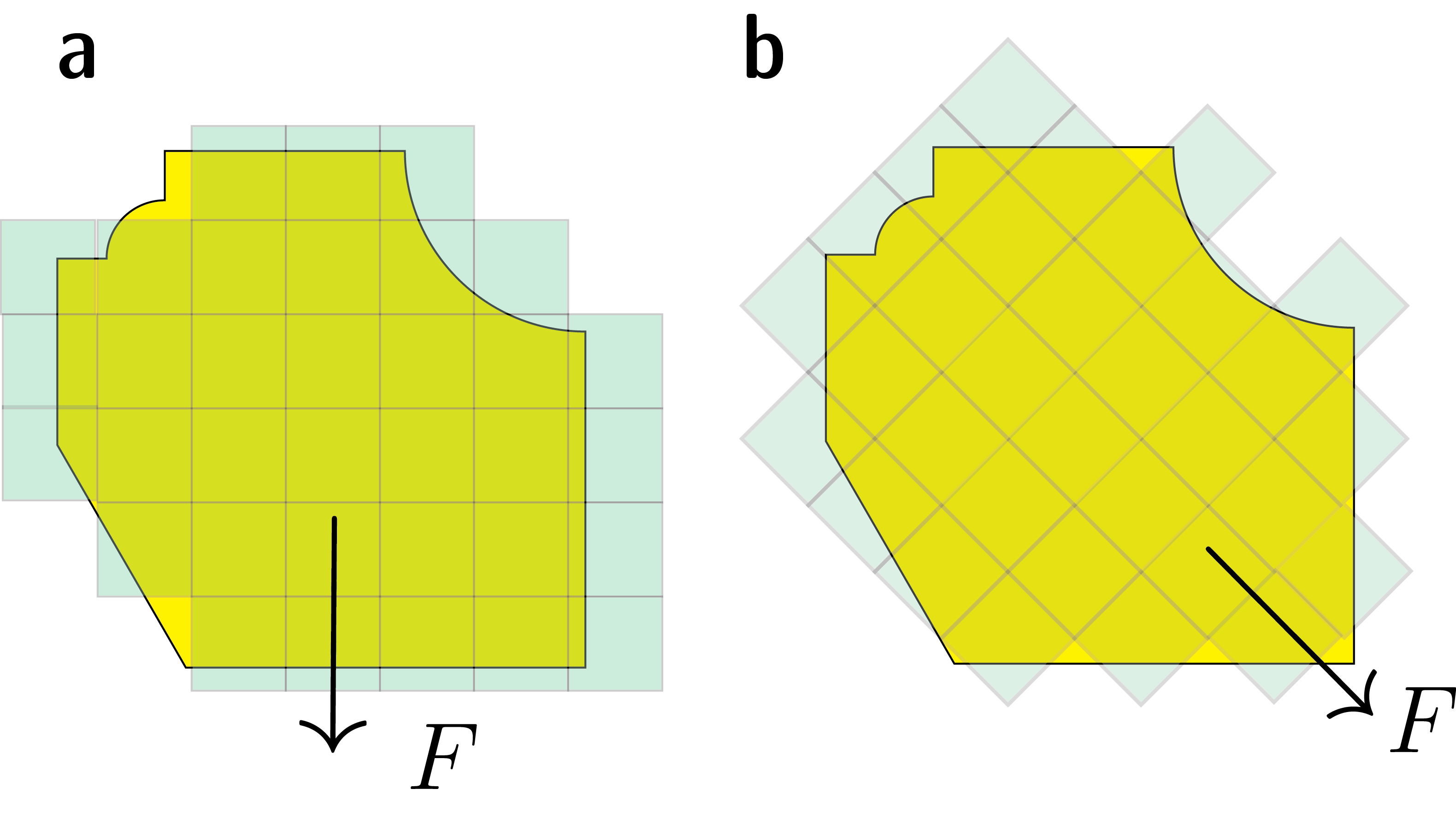
Figure 9: Isotropy of frictional response. The figure show a flat, irregularly shaped, yellow object, with piecewise smooth outer boundary, for which we assume that the ratio of the area of the object to the perimeter of the object is small, and whose boundary is not ‘too jagged’. A tangent force $F$ is applied in two different directions in parts (a) and (b) of the figure. Let the object be approximated by a union of squares joined together, oriented according to the direction of the applied force. As the size of the squares is made arbitrarily small, the area of object gets approximated by the total area of the squares to any desired precision. At the same time, the outer perimeter of the assembly of squares approximates the perimeter of the block within a factor of $\sqrt{2}$ (a factor which comes from the worst case scenario of approximating an edge at an angle of $45^{\circ}$ to the direction of $F$). Hence if the ratio of the area of the object to the perimeter of the object is small, then the ratio of the total area of the assembly of squares to the outer perimeter of the assembly of squares is again small. The imaginary edges of the squares which are glued to each other have no physical existence, and hence they have no effect on the friction. This implies that the two assemblies of squares, and hence the object, have the same frictional response in (a) and (b).

5. Dumbbell. A dumbbell, made by joining two balls, can roll under a torque. In this case, the regions $\mathcal{A}$ and $\mathcal{B}$ in $E_{2}$ are determined by four constants $\mu^{stat}_{s},\,\mu^{stat}_{r},\,\mu^{dyn}_{s},\,\mu^{dyn}_{r}$, with $0<\mu^{dyn}_{r}<\mu^{stat}_{r}\ll\mu^{dyn}_{s}<\mu^{stat}_{s}$. The definition and significance of these constants is explained in the Appendix A of Ghosh et al. (2016). The region $\mathcal{A}$ can be described as follows. Let $\epsilon^{stat}=\arcsin(\mu^{stat}_{r}/\mu^{stat}_{s})$. A point $(r,\theta)\in E_{2}$ with $\pi/2-\epsilon\leq\theta_{obj}\leq\pi/2+\epsilon$ or $\pi/2+\epsilon\leq\theta_{obj}\leq 3\pi/2-\epsilon$ lies in $\mathcal{A}$ if $r|\cos\theta|\leq\mu^{stat}_{r}$. A point $(r,\theta)\in E_{2}$ with $\pi/2-\epsilon\leq\theta_{obj}\leq\pi/2+\epsilon$ or $3\pi/2-\epsilon\leq\theta_{obj}\leq 3\pi/2+\epsilon$ lies in $\mathcal{A}$ if $r\leq\mu^{stat}_{s}$. The theoretical expectation for the shape of the region $\mathcal{B}$ is given by replacing the static coefficients by their dynamic counterparts, and correspondingly replacing the constant $\epsilon^{stat}$. The experimental plots of $\mathcal{A}$ (made with an inclined plane as well as a rotating cylinder) and the plot of $\mathcal{B}$ (made with a rotating cylinder), are consistent with the above for moderate values of $\theta$. On the other hand, a moving dumbbell for which $\theta$ is close to $\pm\pi/2$ (which therefore slides more than it rolls) tends to change its value of $\theta_{obj}$ towards $0$ or $\pi$ as it slows down because of the torque produced by differential normal and tangent forces on the two balls as well as due to mechanical irregularities. Consequently, our experimental plots of the regions $\mathcal{A}$ and $\mathcal{B}$ in Fig. 8 are not closed when $\theta$ is close to $\pm\pi/2$). Noise (produced by the apparatus which raises the plane or rotates the cylinder) is constantly present in the experiments, so a dumbbell begins to move when it is somewhere within the region $\mathcal{C}$, instead of starting from a point of $\partial\mathcal{A}$. The momentum of the moving dumbbell leads to its stopping somewhere inside the region $\mathcal{B}$, instead of stopping exactly on crossing $\partial\mathcal{B}$.

Universal property of the phase spaces of friction

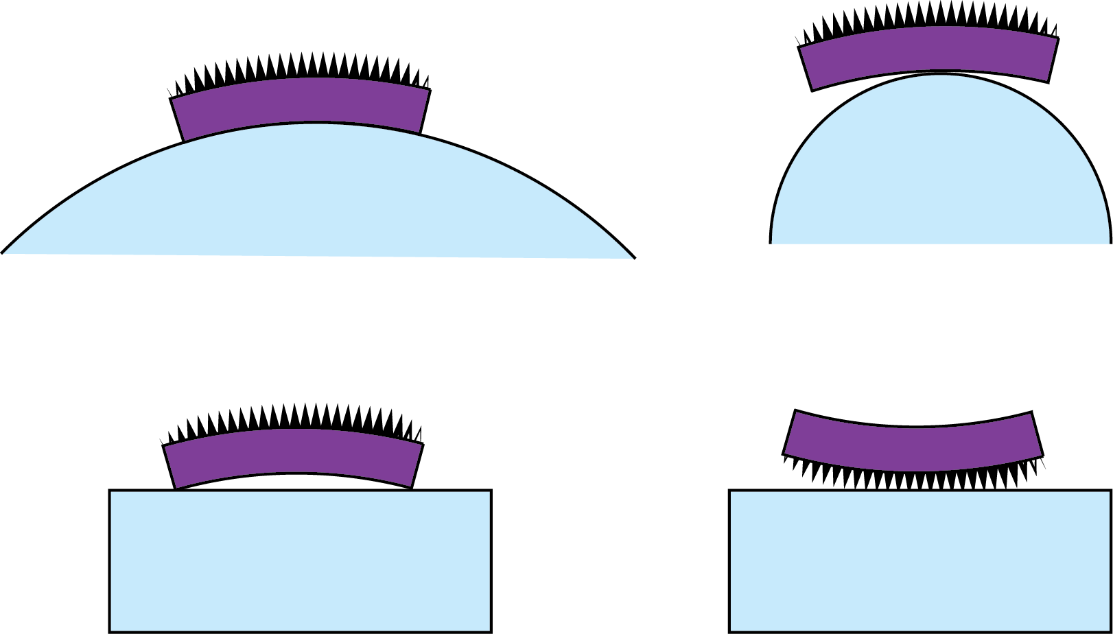
Figure 10: Examples of different natures of contact. The four panels of this figure schematically show an object $O$ coloured purple resting on different substrates made from the same material $M$ coloured blue, such that the nature of contact is different in each panel. Therefore, there will be four different phase spaces $(X,\mathcal{A},\mathcal{B})$ for these arrangements, in which the underlying space $X$ will be the same but the $\mathcal{A}$’s and $\mathcal{B}$’s will change.

Consider any experimental arrangement, in which a chosen object $O$ is pressed against a surface made with material $M$, with a normal force $N$ and subjected to a tangent force $F$, which may depend on the configuration of the object (its position and placement on the surface). We do not need to assume that the surface is flat, but we must require that the nature of the contact between the object and the surface is of a chosen sort (the Fig. 10 explicates with an example the concept of the ‘nature of the contact’). Suppose that the surface is homogeneous, but not necessarily isotropic. If it is not isotropic, let a unit tangent vector field $V$ on the surface encode the possible directionality of the substrate (no such $V$ is to be given if the surface is isotropic). Let there be fixed a fiducial vector on the object. Then from the control parameter space $S$ of the object, we get a classifying map $\psi:S\to X_{4}$ to the phase space $X_{4}$ which sends a point of $S$ to the data $(\lvert N\rvert,\lvert F\rvert/\lvert N\rvert,\theta_{obj},\phi)$ for the configuration given by that point. If the surface is isotropic, we instead consider a map to $Y_{3}$. If we leave out $\lvert N\rvert$ we get a map to $X_{3}$, etc. The phase spaces, together with their regions $\mathcal{A}$ and $\mathcal{B}$, have the universal property that under the classifying map $\psi$, the inverse images of $\mathcal{A}$ and $\mathcal{B}$ are the corresponding empirically determinable regions in the control parameter space $S$, where the object is in the stuck phase, and in the strongly stuck phase, respectively.

Examples of the above for three different experiments with a dumbbell are given in Fig. 8. In other words, once we know by experimenting (say, by using an inclined plane) the regions $\mathcal{A}$ and $\mathcal{B}$ in the phase space, the corresponding regions $\mathcal{A}$ and $\mathcal{B}$ in any other experimental set-up (whose control parameter space is $S$) can just be read off from the regions in the phase space by using the classifying map $\psi:S\to X$ without once again performing the experiments in the new arrangement. Thus, we can get the regions $\mathcal{A}$ and $\mathcal{B}$ for any experimental arrangement from the universal regions $\mathcal{A}$ and $\mathcal{B}$ in phase space, by simply determining the classifying map to the appropriate space. This is what is meant by the universal property of these spaces $X_{4}$ etc. as phase spaces of friction.

When the object $O$ and the material $M$ (and the nature of contact) are altered, we will get new regions $\mathcal{A}^{\prime}$ and $\mathcal{B}^{\prime}$ even if $X$ remains the same, giving a new phase space $(X,\mathcal{A}^{\prime},\mathcal{B}^{\prime})$.

It is possible to extend the construction of phase spaces of friction together with their universal subregions, which will have a universal property, to experiments with composite objects, where the object has multiple parts which are joined by hinges, springs, etc. We can also increase the dimension of $X$ to incorporate the effect of ageing of contact, as well as to incorporate a continuously variable nature contact. Also note that the classifying map $\psi:S\to X$ to the phase space $X$ preserves the symmetries of the experimental set-up, that is, symmetries of $S$, and so it descends to a map $\overline{\psi}:S/G\to X$ on the quotient space $S/G$ of $S$ by the group $G$ of all symmetries of the experimental set-up. This was used above for the experiment with an inclined plane (where there is an action of $G=\mathbb{R}^{2}$ by translation) and for a cylinder (where there is an action of $G=\mathbb{R}$ by translation along the axis), and what we have actually depicted in Fig. 8 are the respective maps $\overline{\psi}:S/G\to X$.

References

- Miguel and Rubi (2006) C. Miguel and M. Rubi, Jamming, yielding, and irreversible deformation in condensed matter, Vol. 688 (Springer, 2006).
- Blatter et al. (1994) G. Blatter, M. V. Feigel’man, V. B. Geshkenbein, A. I. Larkin, and V. M. Vinokur, Reviews of Modern Physics 66, 1125 (1994).
- Van Hecke (2009) M. Van Hecke, Journal of Physics: Condensed Matter 22, 033101 (2009).
- Reichhardt and Reichhardt (2016) C. Reichhardt and C. O. Reichhardt, Reports on Progress in Physics 80, 026501 (2016).
- Kumar et al. (2013) D. Kumar, S. Bhattacharya, and S. Ghosh, Soft Matter 9, 6618 (2013).
- Tomlinson (1929) G. Tomlinson, The London, Edinburgh, and Dublin philosophical magazine and journal of science 7, 905 (1929).
- McClelland and Glosli (1992) G. M. McClelland and J. N. Glosli, in Fundamentals of friction: macroscopic and microscopic processes (Springer, 1992) pp. 405–425.
- Weiss and Elmer (1996) M. Weiss and F.-J. Elmer, Physical review B 53, 7539 (1996).
- Caroli and Nozieres (1996) C. Caroli and P. Nozieres, in Physics of sliding friction (Springer, 1996) pp. 27–49.
- Bowden and Tabor (2001) F. P. Bowden and D. Tabor, The friction and lubrication of solids, Vol. 1 (Oxford university press, 2001).
- Greenwood and Williamson (1966) J. Greenwood and J. Williamson, in Proceedings of the Royal Society of London A: Mathematical, Physical and Engineering Sciences, Vol. 295 (The Royal Society, 1966) pp. 300–319.
- Woydt and Wäsche (2010) M. Woydt and R. Wäsche, Wear 268, 1542 (2010).
- Rabinowicz (1958) E. Rabinowicz, Proceedings of the Physical Society 71, 668 (1958).
- Pabst et al. (2009) S. Pabst, B. Thomaszewski, and W. Strasser, in Proceedings of the 2009 ACM SIGGRAPH/Eurographics Symposium on Computer Animation (ACM, 2009) pp. 149–154.
- Yu et al. (2014) C. Yu, H. Yu, G. Liu, W. Chen, B. He, and Q. J. Wang, Tribology Letters 53, 145 (2014).
- Yu and Wang (2012) C. Yu and Q. J. Wang, Scientific reports 2, 988 (2012).
- Sharma et al. (2008) P. Sharma, S. Ghosh, and S. Bhattacharya, Nature Physics 4, 960 (2008).
- Ruina (1983) A. Ruina, Journal of Geophysical Research: Solid Earth 88, 10359 (1983).
- Persson (1997) B. Persson, Sliding friction: physical principles and applications (Springer Science & Business Media, 1997).
- Ghosh et al. (2016) S. Ghosh, A. Merin, S. Bhattacharya, and N. Nitsure, arXiv preprint arXiv:1605.04438 (2016).
- Homola et al. (1990) A. M. Homola, J. N. Israelachvili, P. M. McGuiggan, and M. L. Gee, Wear 136, 65 (1990).
- Nilsson et al. (2009) D. Nilsson, P.