Variational Principle for Stars with a Phase Transition

Institute for Theoretical and Experimental Physics, ul. Bolshaya Cheremushkinskaya 25, Moscow, 117218 Russia¹
Novosibirsk State University, ul. Pirogova 2, Novosibirsk, 630090 Russia²
‘‘Kurchatov Institute’’ National Research Center, pl. Kurchatova 1, Moscow, 123182 Russia³

The variational principle for stars with a phase transition has been investigated. The term outside the integral in the expression for the second variation of the total energy of a star is shown to be obtained by passage to the limit from the integration over the region of mixed states in the star. The form of the trial functions ensuring this passage has been found. All of the results have been generalized to the case where general relativity is applicable. The known criteria for the dynamical stability of a star when a new phase appears at its center are shown to follow automatically from the variational principle. Numerical calculations of hydrostatically equilibrium models for hybrid stars with a phase transition have been performed. The form of the trial functions for the second variation of the total energy of a star that describes almost exactly the stability boundaries of such stellar models is proposed.

Keywords: stability of stars, phase transition, variational principle.

 
^∗ e-mail: $<$yudin@itep.ru$>$

INTRODUCTION

The necessity of estimating the stability of a stellar configuration often arises in various problems of astrophysics. The variational principle (VP) allows one to obtain not only the hydrostatic equilibrium equations for a star from the condition for its total energy, the sum of its gravitational and internal energies, being extremal, but also the condition for the dynamical stability of this equilibrium that ensures a minimum of the total energy (see Zel’dovich and Novikov 1967). In this case, the stability condition is written as the requirement that the second variation of the integral of the total energy be positive for the entire set of trial functions describing the various perturbation modes. However, in the case of a limited number of trial functions used, the VP gives a necessary but not sufficient condition for the stability of a star: if the star is stable for a given perturbation (a given form of the trial function), then this by no means guarantees its absolute stability. As experience shows, for practical purposes it is sometimes sufficient to check the stability of a star to the simplest perturbations; in particular, a good approximation for a star without phase transitions is the investigation of its stability with respect to homogeneous deformation along the radius $r$: $\delta r\sim r$. This leads to a well-known stability condition for the adiabatic index $\gamma$ averaged over the star: $\langle\gamma\rangle>4/3$, where the averaging is over the mass coordinate with weight $P/\rho$, while $P$ and $\rho$ are the pressure and density in the matter, respectively. Thus, the variational principle is an efficient method for a practical estimation of the stability of stars.

THE VARIATIONAL PRINCIPLE IN THE NONRELATIVISTIC REGION

Let us first consider the simplest phase transition (PT): a Maxwellian PT (a typical example is the liquid–gas transition in homogeneous matter). In this case, the phase equilibrium conditions lead to the equality $\left(\frac{\partial P}{\partial\rho}\right)_{\!\!T}=0$ in the phase coexistence region. Let also, for simplicity, the temperature $T=0$. Under these conditions there is no region of mixed states in the star, the phases are strictly spatially separated, and a density jump occurs at the the phase boundary. The variational principle for a star with such a phase transition was obtained within the framework of Newtonian gravity by Bisnovatyi-Kogan et al. (1975) (see also Bisnovatyi-Kogan 1989):

$$\mathbf{V}=\mathbf{V}_{\mathrm{I}}+\mathbf{V}_{\mathrm{O}}=\int\limits_{0}^{M}\left[P\gamma\rho\left(\frac{d\varphi}{dm}\right)^{2}-\frac{4\beta}{9}\frac{m\varphi^{2}}{\upsilon^{7/3}}\right]dm+\frac{\beta m_{*}}{3\upsilon_{*}^{4/3}}\frac{(\varphi_{1}-\varphi_{2})^{2}}{\frac{1}{\rho_{1}}-\frac{1}{\rho_{2}}}>0,$$ (1)

where $\beta=G(4\pi/3)^{1/3}$ and $\upsilon=4\pi r^{3}/3$. It is convenient to use the quantity $\upsilon$ rather than directly $r$ due to the relation $dm=\rho d\upsilon$. The integration in (1) is over the mass coordinate $m$ in a hydrostatically equilibrium star, $M$ is the total mass of the star, $\varphi=\varphi(m)$ is the trial function (different at different phases, the phases are numbered from the stellar surface) that describes some perturbation $\delta\upsilon=\varepsilon\varphi(m)$, $\varepsilon$ is an infinitesimal quantity. As can be seen from (1), in the presence of a phase transition $\mathbf{V}$ is the sum of two parts: the integral $\mathbf{V}_{\mathrm{I}}$ and outside the integral $\mathbf{V}_{\mathrm{O}}$. The term outside the integral contains the mass coordinate $m_{*}$ and the volume $\upsilon_{*}$ at the density jump from $\rho_{1}$ to $\rho_{2}$, $\rho_{1}<\rho_{2}$. If there are several phase transitions, then each one has its own corresponding term outside the integral of the same form.

The Phase Transition at the Stellar Center

It follows from the condition for the variations $\delta r,\ \delta\rho$, etc. being bounded that for the central phase (this is phase 2 in the case of one PT) $\varphi_{2}(0)=0$. In this case, the trial functions are not continuous at the phase boundaries; therefore, if the PT occurs near the stellar center, then the contribution to $\mathbf{V}$ from phase 1 under the condition $\varphi_{1}(m_{*})\neq 0$ is decisive. Indeed, the term outside the integral at $m_{*}\approx\rho_{\mathrm{2}}\upsilon_{*}$, where $\rho_{2}\approx\rho_{\mathrm{c}}$ is the density at the stellar center, tends to

$$\frac{\rho_{\mathrm{2}}}{3\upsilon_{*}^{1/3}}\frac{\varphi_{1}^{2}(0)}{\frac{1}{\rho_{1}}{-}\frac{1}{\rho_{2}}}$$ (2)

and diverges as $1/\upsilon_{*}^{1/3}$ when $\upsilon_{*}\rightarrow 0$. The second term, which after the integration is also of order $O(1/\upsilon_{*}^{1/3})$, is decisive in the integral. Let us transform the expression for $\mathbf{V}_{\mathrm{I}}$ so as to gather all divergences outside the integral. For this purpose, let us integrate the second term in $\mathbf{V}_{\mathrm{I}}$ twice by parts. We will then obtain $\mathbf{V}=\widetilde{\mathbf{V}}_{\mathrm{I}}+\widetilde{\mathbf{V}}_{\mathrm{O}}$, where we separated out the new integral part

$$\widetilde{\mathbf{V}}_{\mathrm{I}}=\int\limits_{0}^{M}\left[P\gamma\rho\left(\frac{d\varphi}{dm}\right)^{2}-\frac{\beta m}{3\upsilon^{4/3}}\!\!\left\{\frac{d(\rho\varphi^{2})}{dm}+\frac{3\upsilon}{m}\frac{d(\rho^{2}\varphi^{2})}{dm}\right\}\right]dm,$$ (3)

and the part outside the integral:

$$\widetilde{\mathbf{V}}_{\mathrm{O}}=\frac{\beta}{3\upsilon_{*}^{4/3}}\!\left\{m_{*}\frac{(\varphi_{1}\rho_{1}{-}\varphi_{2}\rho_{2})^{2}}{\rho_{2}-\rho_{1}}+3\upsilon_{*}\left[(\varphi_{2}\rho_{2})^{2}{-}(\varphi_{1}\rho_{1})^{2}\right]\right\}.$$ (4)

As before, if there are several PTs, then each one has its own corresponding contribution to $\mathbf{V}$ of form (4). Let now the PT occurs near the center. Then, $\widetilde{\mathbf{V}}_{\mathrm{I}}=O(1)$ and $\widetilde{\mathbf{V}}_{\mathrm{O}}=O(1/\upsilon_{*}^{1/3})$. Given that $\varphi_{2}\rightarrow 0$, $\varphi_{1}=O(1)$, and $m_{*}\approx\rho_{2}\upsilon_{*}$, we will obtain the stability condition in a well-known form (see Lighthill 1950):

$$\frac{\rho_{2}}{\rho_{1}}<\frac{3}{2}.$$ (5)

The Origin of the Term Outside the Integral

The variational principle expressed by Eq. (1) is applicable only for stars in which the phases are separated spatially and have a well-defined boundary at which the term outside the integral is calculated. However, what to do in the case where the phase coexistence region is present in the star and, consequently, the density graph has the pattern of a smoothed step or an even smoother transition? This can be true both for the Maxwellian description of the PT, in the case where the star has a nonzero temperature whose gradient ensures a hydrostatic equilibrium of the phase coexistence region, and for the Gibbs description, when $\left(\frac{\partial P}{\partial\rho}\right)_{\!\!T}>0$ even at $T=0$. In this case, the condition for positivity of the second variation of the star’s energy, from which the variational principle follows, gives only the integral part of Eq. (1). Let us trace how the term outside the integral appears when passing to the limit of a strict spatial phase separation (see the Appendix in Bisnovatyi-Kogan et al. (1975)).

Thus, let we have a stellar configuration with a comparatively narrow phase coexistence zone. We will consider the Maxwellian description of the PT and assume the zone of mixed states to be described by an isentrope. This assumption is quite natural: first, due to the possible action of convection and, second, due to the presumed narrowness of the spatial region under consideration. We will then obtain the limit of cold matter by letting the entropy $S$ approach zero. Let us separate out the contribution to $\mathbf{V}$ from the zone of mixed states. The contribution from the second term in the integrand in (1), in view of its boundedness, approaches zero when $S\rightarrow 0$ and $\triangle m\rightarrow 0$, where $\triangle m$ is the width of the domain of integration in the star. Therefore, we can write

$$\triangle\mathbf{V}\approx\int\limits_{\mathrm{mix}}P\gamma\rho\left(\frac{d\varphi}{dm}\right)^{2}dm,$$ (6)

where the integral is taken over the phase coexistence region.

Let us now consider the behavior of the parameters of matter on the isentrope in the region of mixed states. The phase equilibrium conditions are reduced to the equality of their pressures and chemical potentials:

$$\left\{\begin{aligned} P_{1}&=P_{2},\\ \mu_{1}&=\mu_{2},\end{aligned}\right.$$ (7)

where the index numbers the phases. The entropy and density are expressed via the mixing parameter $0\leq\chi\leq 1$ (equal to the mass fraction of the phases) as

$$S =\chi S_{1}+(1{-}\chi)S_{2},$$ (8)

$$\sigma =\chi\sigma_{1}+(1{-}\chi)\sigma_{2}.$$

Here, for convenience, we have introduced a quantity $\sigma\equiv 1/\rho$ that, to within a factor, has the meaning of volume per unit baryonic charge. For the changes in these quantities on the isentrope we have

$$\delta S =(S_{1}-S_{2})\delta\chi+\left[\chi\left(\frac{\partial S_{1}}{\partial T}\right)_{\!\!\mathrm{pt}}+(1{-}\chi)\left(\frac{\partial S_{2}}{\partial T}\right)_{\!\!\mathrm{pt}}\right]\delta T=0,$$ (9)

$$\delta\sigma =(\sigma_{1}-\sigma_{2})\delta\chi+\left[\chi\left(\frac{\partial\sigma_{1}}{\partial T}\right)_{\!\!\mathrm{pt}}+(1{-}\chi)\left(\frac{\partial\sigma_{2}}{\partial T}\right)_{\!\!\mathrm{pt}}\right]\delta T.$$ (10)

In these expressions the first and second terms describe, respectively, the change due to the redistribution of matter between the phases and due to the change in phase equilibrium conditions. Here, we have also introduced the notation for the differential operator

$$\left(\frac{\partial}{\partial T}\right)_{\!\!\mathrm{pt}}\equiv\left(\frac{\partial}{\partial T}\right)_{\!\!P}+\left(\frac{\partial P}{\partial T}\right)_{\!\!\mathrm{pt}}\left(\frac{\partial}{\partial P}\right)_{\!\!T}.$$ (11)

The quantity $\left(\frac{\partial P}{\partial T}\right)_{\!\!\mathrm{pt}}$ is found directly from the equilibrium conditions (7) (the Clayperon–Clausius formula):

$$\left(\frac{\partial P}{\partial T}\right)_{\!\!\mathrm{pt}}=\frac{S_{1}-S_{2}}{\sigma_{1}-\sigma_{2}}.$$ (12)

Combining Eqs. (9), (10) and (12), we obtain

$$P\rho\gamma=-\left(\frac{\partial P}{\partial\sigma}\right)_{\!\!S}=\frac{\left(\frac{\partial P}{\partial T}\right)_{\!\!\mathrm{pt}}^{2}}{\chi S_{\mathrm{T1}}+(1{-}\chi)S_{\mathrm{T2}}}.$$ (13)

As can be seen, the quantity $S_{\mathrm{T}}$ introduced here,

$$S_{\mathrm{T}}\equiv\left(\frac{\partial S}{\partial T}\right)_{\!\!\mathrm{pt}}-\left(\frac{\partial\sigma}{\partial T}\right)_{\!\!\mathrm{pt}}\left(\frac{\partial P}{\partial T}\right)_{\!\!\mathrm{pt}}=\left(\frac{\partial S}{\partial T}\right)_{\!\!\rho}-\left(\frac{\partial\sigma}{\partial P}\right)_{\!\!T}\left[\left(\frac{\partial P}{\partial T}\right)_{\!\!\rho}-\left(\frac{\partial P}{\partial T}\right)_{\!\!\mathrm{pt}}\right]^{2},$$ (14)

is strictly positive due to the thermodynamic inequalities

$$\left(\frac{\partial S}{\partial T}\right)_{\!\!\rho}\geq 0,\quad\left(\frac{\partial P}{\partial\sigma}\right)_{\!\!T}\leq 0.$$ (15)

The hydrostatic equilibrium equation for a star

$$\frac{dP}{dm}=\left(\frac{\partial P}{\partial T}\right)_{\!\!\mathrm{pt}}\frac{dT}{dm}=-\frac{\beta m}{3\upsilon^{4/3}},$$ (16)

gives a relation between $T$ and $m$, while Eq. (9) gives a relation between $T$ and $\chi$:

$$\left(\frac{\partial T}{\partial\chi}\right)_{\!\!S}=-\frac{S_{1}-S_{2}}{\chi\left(\frac{\partial S_{1}}{\partial T}\right)_{\!\!\mathrm{pt}}+(1{-}\chi)\left(\frac{\partial S_{2}}{\partial T}\right)_{\!\!\mathrm{pt}}}.$$ (17)

Gathering now Eqs. (13), (16), and (17), given (12), we obtain

$$\triangle\mathbf{V}=\int\limits_{0}^{1}\left(\frac{\partial\varphi}{\partial\chi}\right)_{\!\!}^{\!\!2}\left[\frac{\chi\left(\frac{\partial S_{1}}{\partial T}\right)_{\!\!\mathrm{pt}}+(1{-}\chi)\left(\frac{\partial S_{2}}{\partial T}\right)_{\!\!\mathrm{pt}}}{\chi S_{\mathrm{T1}}+(1{-}\chi)S_{\mathrm{T2}}}\right]\frac{\beta m\ d\chi}{3\upsilon^{4/3}(\sigma_{1}{-}\sigma_{2})}.$$ (18)

$S_{\mathrm{T}}\rightarrow\left(\frac{\partial S}{\partial T}\right)_{\!\!\mathrm{pt}}$ when $T\rightarrow 0$, and the expression in square brackets in (18) tends to unity, while all the remaining quantities, except the term with $\varphi$, can be taken outside the integral sign, because they are almost constant in the domain of integration due to its narrowness. Only the expression

$$\int\limits_{0}^{1}\left(\frac{d\varphi}{d\chi}\right)^{2}d\chi.$$ (19)

remains under the integral. At fixed values of the trial function $\varphi_{1}$ and $\varphi_{2}$ at the phase boundaries, as is easy to show, the minimum of the integral (of interest to us) is ensured by the linear function $\varphi=\varphi_{1}\chi+\varphi_{2}(1{-}\chi)$, while the integral (19) itself is equal to $(\varphi_{1}{-}\varphi_{2})^{2}$, i.e., $\triangle\mathbf{V}$ from (6) turns into the term outside the integral $\mathbf{V}_{\mathrm{O}}$ from (1). Thus, the first term in the integral of the variational principle when $T\rightarrow 0$ plays the role of a delta function and, despite the narrowing of the domain of integration $\triangle m\rightarrow 0$, gives rise to a finite term outside the integral.

THE VARIATIONAL PRINCIPLE IN GENERAL RELATIVITY

Let us write the stellar equilibrium equations (the Tolman–Oppenheimer–Volkoff equations) in general relativity (GR):

$$\frac{dP}{dr} =-\frac{Gm(\epsilon+P)}{r^{2}c^{2}}\frac{1+\frac{4\pi Pr^{3}}{mc^{2}}}{1-\frac{2Gm}{rc^{2}}},$$ (20)

$$\frac{dm}{dr} =4\pi r^{2}\frac{\epsilon}{c^{2}}.$$ (21)

Here, $\epsilon$ is the energy of matter per unit volume (including the rest energy). The condition for the stability of a star is written in GR via the variational principle as (see Wheeler et al. 1967; Bisnovatyi-Kogan 1968)

$$\mathbf{V}=4\pi e^{-\Phi(R)}\int\limits_{0}^{R}e^{\Phi(r)}\left[I_{1}+I_{2}+I_{3}\right]dr\geq 0,$$ (22)

where

$$\Phi(\widetilde{r})=\int\limits_{0}^{\widetilde{r}}\frac{P+\epsilon}{1-\frac{2Gm}{rc^{2}}}\frac{4\pi Gr}{c^{4}}dr.$$ (23)

The terms under the integral are

$$I_{1} =\gamma P\left[2\delta r+r\frac{d\delta r}{dr}-\frac{Gm}{rc^{2}}\frac{1+\frac{4\pi r^{3}P}{mc^{2}}}{1-\frac{2Gm}{rc^{2}}}\delta r\right]^{2},$$ (24)

$$I_{2} =-\frac{P+\epsilon}{\left(1-\frac{2Gm}{rc^{2}}\right)^{2}}\left(1+\frac{4\pi r^{3}P}{mc^{2}}\right)^{2}\left(\frac{Gm}{rc^{2}}\right)^{2}\delta r^{2},$$

$$I_{3} =-\frac{P+\epsilon}{\left(1-\frac{2Gm}{rc^{2}}\right)}\left(1+\frac{2\pi r^{3}P}{mc^{2}}\right)\frac{4Gm}{rc^{2}}\delta r^{2}.$$

As above, let us introduce a variable $\upsilon=4\pi r^{3}/3$, $\delta\upsilon=\varepsilon\varphi(m)$ (recall that $\varepsilon$ is an infinitesimal), and dimensionless combinations

$$p\equiv\frac{P}{\epsilon},\quad q\equiv\frac{4\pi r^{3}P}{mc^{2}},\quad\tau\equiv\frac{Gm}{rc^{2}}.$$ (25)

Passing to the integration over the mass coordinate, we then obtain

$$\Phi(\widetilde{m})=\int\limits_{0}^{\widetilde{m}}\frac{\tau(1+p)}{(1-2\tau)}\frac{dm}{m}.$$ (26)

The variational integral takes the form

$$\mathbf{V}=e^{-\Phi(M)}\int\limits_{0}^{M}e^{\Phi(m)}\left[\widetilde{I}_{1}+\widetilde{I}_{2}+\widetilde{I}_{3}\right]dm,$$ (27)

where

$$\widetilde{I}_{1} =\gamma P\frac{\epsilon}{c^{2}}\left[\frac{d\varphi}{dm}-\frac{p\tau(1+q)}{q(1-2\tau)}\frac{\varphi}{m}\right]^{2},$$ (28)

$$\widetilde{I}_{2}+\widetilde{I}_{3} =-P\frac{\epsilon}{c^{2}}\left[4+2q+\frac{\tau}{1{-}2\tau}(1+q)^{2}\right]\frac{\tau p(1+p)}{1-2\tau}\left(\frac{\varphi}{mq}\right)^{2}.$$ (29)

It is easy to see that in the nonrelativistic case, $q\ll 1$, $p\ll 1$ and $\tau\ll 1$, these expressions give the Newtonian limit (1).

The Term Outside the Integral in GR

Let us find the form of the term outside the integral in GR. As in the Newtonian case, it arises from the integral over the zone of mixed states in the limit $T\rightarrow 0$. In this case,

$$\triangle\mathbf{V}\approx e^{-\Phi(M)}\int\limits_{\mathrm{mix}}e^{\Phi(m)}\gamma P\frac{\epsilon}{c^{2}}\left(\frac{d\varphi}{dm}\right)^{2}dm.$$ (30)

Repeating the reasoning that led us to Eq. (18), with the only difference that the equilibrium equations are now given by the relativistic expressions (20)–(21), we will obtain

$$\triangle\mathbf{V}\approx e^{-\Phi(M)}\int\limits_{0}^{1}\frac{e^{\Phi(m)}}{\left(\frac{\partial\sigma}{\partial\chi}\right)_{\!\!S}}\frac{P+\epsilon}{\rho c^{2}}\left(\frac{d\varphi}{d\chi}\right)^{2}\frac{Gm}{4\pi r^{4}}\frac{1+\frac{4\pi r^{3}P}{mc^{2}}}{1-\frac{2Gm}{rc^{2}}}d\chi.$$ (31)

Recall that $\sigma\equiv 1/\rho$. For $T\rightarrow 0$

$$\left(\frac{\partial\sigma}{\partial\chi}\right)_{\!\!S}\approx\frac{1}{\rho_{1}}-\frac{1}{\rho_{2}},$$ (32)

while $\frac{P+\epsilon}{\rho}$ coincides, to within a factor, with the chemical potential of matter (see Eq. (44) below) and, hence, is continuous at the phase transition. Therefore,

$$\frac{P+\epsilon}{\rho\left(\frac{\partial\sigma}{\partial\chi}\right)_{\!\!S}}=\frac{1}{\frac{1}{P+\epsilon_{1}}-\frac{1}{P+\epsilon_{2}}}.$$ (33)

All of the slowly changing factors can now be taken outside the integral sign. Repeating the reasoning of the Newtonian case, we again conclude that the trial function depends linearly on the mixing parameter in the phase coexistence region. Finally, for the term outside the integral $\mathbf{V}_{\mathrm{O}}=\triangle\mathbf{V}$ in GR we have

$$\mathbf{V}_{\mathrm{O}}=\frac{Gm_{*}}{4\pi r_{*}^{4}}\frac{(\varphi_{1}-\varphi_{2})^{2}}{\left[\frac{c^{2}}{P_{*}+\epsilon_{1}}-\frac{c^{2}}{P_{*}+\epsilon_{2}}\right]}\frac{1+\frac{4\pi r_{*}^{3}P_{*}}{m_{*}c^{2}}}{1-\frac{2Gm_{*}}{r_{*}c^{2}}}e^{\Phi(m_{*})-\Phi(M)},$$ (34)

where, as above, the symbol $*$ denotes the PT position. As it must be, we obtain the term outside the integral from (1) in the Newtonian limit. Using the dimensionless parameters (25) introduced above, this expression can also be written as

$$\mathbf{V}_{\mathrm{O}}=\frac{P_{*}^{2}}{m_{*}c^{2}}\frac{(\varphi_{1}-\varphi_{2})^{2}}{\left[\frac{p_{1}}{1+p_{1}}-\frac{p_{2}}{1+p_{2}}\right]}\frac{\tau_{*}(1+q_{*})}{q_{*}(1-2\tau_{*})}e^{\Phi(m_{*})-\Phi(M)}.$$ (35)

The Stability Condition at the PT at the Stellar Center

Let us derive the dynamical stability condition at the PT occurring near the stellar center from the variational principle. According to (34), the term outside the integral diverges as $1/r_{*}$ when $r_{*}\rightarrow 0$, because $\varphi_{2}\rightarrow 0$ and $\varphi_{1}\rightarrow\mathrm{const}\neq 0$. The term $I_{3}$ makes a similar contribution in the integral. Near the center we can write

$$m\approx\frac{4\pi}{3c^{2}}\left[\epsilon_{2}r_{*}^{3}+\epsilon_{1}\left(r^{3}-r_{*}^{3}\right)\right].$$ (36)

Retaining only the divergent terms, we will then obtain

$$\mathbf{V}_{\mathrm{I}}\approx-\frac{G\varphi_{1}^{2}}{3c^{4}r_{*}}(\epsilon_{1}+P_{*})(\epsilon_{2}+3\epsilon_{1}+6P_{*})e^{-\Phi(M)}.$$ (37)

The term outside the integral in the same approximation is

$$\mathbf{V}_{\mathrm{O}}\approx\frac{G\varphi_{1}^{2}}{3c^{4}r_{*}}\frac{\epsilon_{2}+3P_{*}}{\left[\frac{1}{P_{*}+\epsilon_{1}}-\frac{1}{P_{*}+\epsilon_{2}}\right]}e^{-\Phi(M)}.$$ (38)

The stability condition $\mathbf{V}=\mathbf{V}_{\mathrm{I}}+\mathbf{V}_{\mathrm{O}}>0$ then immediately leads to the following relation first derived by Seidov (1971):

$$\frac{\epsilon_{2}}{\epsilon_{1}}<\frac{3}{2}\left(1+\frac{P_{*}}{\epsilon_{1}}\right),$$ (39)

which is a generalization of (5) to the case of GR.

AN EXAMPLE OF APPLYING THE VP

Before turning to the results of our numerical calculations, let us consider a curious example of applying the variational principle. For simplicity, we will work within the framework of Newtonian gravity (the description in GR is similar). Consider the case of weak splitting of one PT into two smaller PTs (see Fig. 1, the splitting size is exaggerated for clarity).

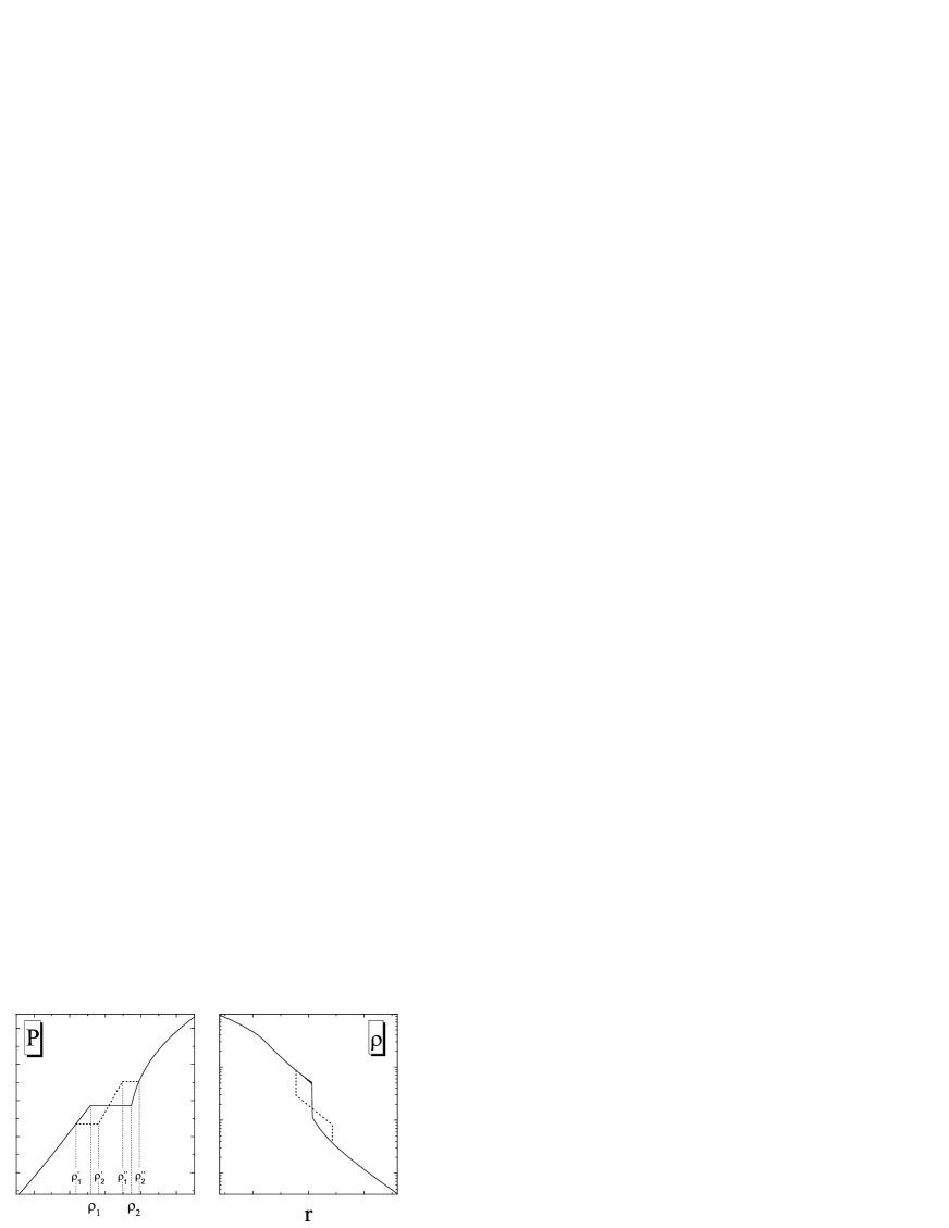
Fig. 1: Left: dependence $P(\rho)$ for one PT (solid curve) and two PTs (dashed curve line). Right: the same for the behavior of $\rho(r)$ in the star.

Let the old values of the PT beginning and end be, as previously, $\rho_{1}$ and $\rho_{2}$, while the new values be $\rho^{\prime}_{1}$, $\rho^{\prime}_{2}$ and $\rho^{\prime\prime}_{1}$, $\rho^{\prime\prime}_{2}$, respectively, with $\rho^{\prime}_{1}\leq\rho_{1}$, $\rho^{\prime\prime}_{2}\geq\rho_{2}$ and $\rho^{\prime}_{2}\leq\rho^{\prime\prime}_{1}$. If the splitting is weak, i.e., $\rho^{\prime}_{1}\approx\rho_{1}$ and $\rho^{\prime\prime}_{2}\approx\rho_{2}$, then the stellar structure changes weakly, while the regions of the density jumps remain at virtually the same values $m_{*}$ and $\upsilon_{*}$. This means that in Eq. (1) for $\mathbf{V}$ the integral part $\mathbf{V}_{\mathrm{I}}$ remains virtually without any changes. Omitting the common factor $\frac{\beta m_{*}}{3\upsilon_{*}^{4/3}}$, let us write the term outside the integral $\mathbf{V^{\prime}}_{\mathrm{\!O}}$ for the case of two PTs:

$$\mathbf{V^{\prime}}_{\mathrm{\!O}}\propto\frac{(\varphi_{1}{-}\varphi_{3})^{2}}{\frac{1}{\rho_{1}}-\frac{1}{\rho_{2}^{\prime}}}+\frac{(\varphi_{3}{-}\varphi_{2})^{2}}{\frac{1}{\rho_{1}^{\prime\prime}}-\frac{1}{\rho_{2}}}\geq\frac{(\varphi_{1}{-}\varphi_{2})^{2}}{\frac{1}{\rho_{1}}-\frac{1}{\rho_{2}}},$$ (40)

where we set $\rho^{\prime}_{1}=\rho_{1}$ and $\rho^{\prime\prime}_{2}=\rho_{2}$ and assume that the third phase is between the first and second ones. The last inequality in (40) implies that we always have $\mathbf{V^{\prime}}_{\mathrm{\!O}}>\mathbf{V}_{\mathrm{O}}$ for the case under consideration and, hence, weak splitting of one PT into two smaller PTs increases the stability margin for the star. This fact can have important consequences when considering the stability of hybrid stars, i.e., stars containing ‘‘exotic’’ phases inside: quarks etc. It may well be that the transition to quark matter can occur not immediately but through a sequence of multi-quark states (see, e.g., Krivoruchenko et al. (2011) and references therein). According to what has been said above, this possibility, if it is realized in nature, can additionally contribute to the stability of hybrid stars.

THE CHOICE OF BASIS FUNCTIONS

To begin with, we need to choose a form of the trial function. In doing so, we want to make sure that our algorithm of using the variational principle is universal and would be suitable both in the case of a sharp boundary between the phases in the star (Maxwellian PT) and in the case of a ‘‘smoothed’’ (Gibbs) PT, where the phases gradually pass into one another and the region of mixed states is clearly present in the star. In the most general case, knowing only the equation of state for matter (i.e., the dependence $P(\rho)$ etc.) without any information about its phase composition must be sufficient for us. Thus, we need the functions common to all phases in the star.

We will seek the trial function $\varphi=\varphi(m)$ as an expansion in terms of basis function $g_{i}(m)$:

$$\varphi(m)=\sum\limits_{i=1}^{N_{\mathrm{g}}}\alpha_{i}g_{i}(m),$$ (41)

where $N_{\mathrm{g}}$ is the number of basis functions. When this expression is substituted into the variational principle, we obtain a stability condition in the form

$$\sum\limits_{i,j=1}^{N_{\mathrm{g}}}M_{ij}\alpha_{i}\alpha_{j}\geq 0,$$ (42)

where the element of the matrix $M_{ij}$ contains both the contributions from the integrals from $\mathbf{V}_{\mathrm{I}}$ with the functions $g_{i}$ and $g_{j}$ and the contributions from the term outside the integral $\mathbf{V}_{\mathrm{O}}$ (where it is present). Consequently, the stability condition is reduced to the requirement that this quadratic (in coefficients $\alpha_{i}$) form be positive definite, which is known to be equivalent to the condition for positivity of all principal minors of the matrix $M_{ij}$.

Our main task is now to find the minimal set of basis functions $g_{i}$ that would describe best the stability of stellar configurations with PTs. Undoubtedly, the list of such functions must include the ‘‘classical’’ function $g_{1}=\upsilon$ that works excellently for stars without PTs. As follows from the previously considered method of deriving the term outside the integral in the VP, the basis function that plays the role of a delta function in the limit $T\rightarrow 0$ must be linear in $\chi$ in the region of mixed states. In addition to the quantities from (8), they also include the internal energy per unit mass $E$:

$$E=\chi E_{1}+(1{-}\chi)E_{2},$$ (43)

which is related to the previously used energy per unit volume $\epsilon$ by the relation $\epsilon=\rho E$ The pressure $P$ and chemical potential $\mu$ experience no jump at the PT, while the entropy becomes zero for cold configurations. This means that we have two possibilities: the basis function must include $E$ or $\sigma=1/\rho$. The relation between all of the functions listed above is clearly illustrated by the basic thermodynamic identity

$$E+\frac{P}{\rho}=TS+\frac{Y\mu}{\mbox{$m_{\mathrm{u}}$}},$$ (44)

where $m_{\mathrm{u}}$ is the atomic mass unit, and $Y$ is the dimensionless concentration. It follows from the condition for the variations at the stellar center being bounded that the basis functions must become zero there, i.e., for example, $E$ must enter into the expression for the trial function as a combination $E{-}E_{\mathrm{c}}$, where $E_{\mathrm{c}}$ is its central value. Besides, the basis function with $\sigma=1/\rho$ must contain the factor removing the singularity on the stellar surface, for example, must be $(M{-}m)/\rho$, where $M$ is the total mass of the star, or $P/\rho-P_{\mathrm{c}}/\rho_{\mathrm{c}}$ etc. In addition, as has already been noted, the basis function can include some smoothly changing factor.

RESULTS OF CALCULATIONS

After some numerical experiments, we chose the following main set of basis functions:

$$\{g_{1},g_{2},g_{3}\}=\left\{\upsilon,\frac{M-m}{\rho}-\frac{M}{\rho_{\mathrm{c}}},E-E_{\mathrm{c}}\right\},$$ (45)

with all of the above reservations. However, this choice is only an example. Here, we set the goal only to demonstrate the efficiency of the variational principle. The question about the choice of a minimal set of optimal trial functions needs to be investigated further.

The Newtonian Case

In the nonrelativistic case, the VP is expressed by Eq. (1). To demonstrate how the VP works, we chose the simplest case of a PT between two polytropes. Polytrope 1 had an index $n_{1}=\frac{1}{\gamma_{1}-1}=3/2$, i.e., $\gamma_{1}=5/3$. The index of the second polytrope $n_{2}=\frac{1}{\gamma_{2}-1}$ was varied. It is easy to show that the phase equilibrium conditions (7) in this case lead to the following relation between the density jump at the PT $\lambda=\rho_{2}/\rho_{1}$ and the adiabatic indices:

$$\lambda=\frac{\gamma_{2}(\gamma_{1}-1)}{\gamma_{1}(\gamma_{2}-1)}.$$ (46)

Thus, a fixed value of $\lambda$ corresponds to each value of $\gamma_{2}$. This makes it possible to compute a one–parameter sequence of models for hydrostatically equilibrium stars with various central densities $\rho_{c}$ and to separate the dynamically stable models from the unstable ones. For the bipolytropic models with $\gamma_{1}=5/3$ and various values of $\gamma_{2}$ considered here, the computed boundary between the stable and unstable models is indicated by the thick solid curve in 2, which is a diagram: the density jump $\lambda$ is along the horizontal axis, and the ratio of the central pressure $P_{c}$ to the pressure at the phase transition $P_{*}$ is along the vertical axis.

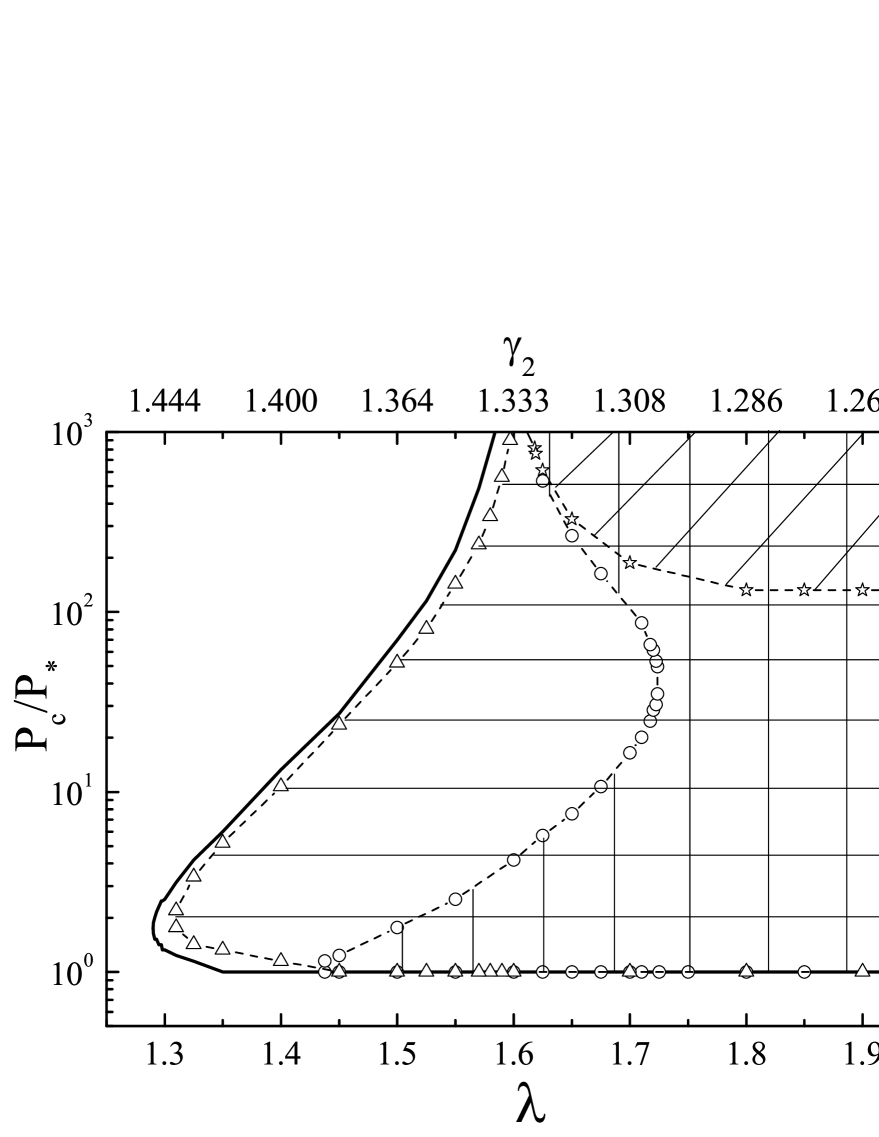
Fig. 2: The $\left(\frac{P_{\mathrm{c}}}{P_{*}},\lambda\right)$ diagram computed within the framework of Newtonian gravity. The curves with symbols indicate the stability boundaries. The oblique, vertical, and horizontal hatching indicates the instability zone according to the variational principle with one, two, and three basis functions, respectively. The real instability region is bounded by the thick solid curve. The values of $\gamma_{2}$ corresponding to given $\lambda$ are shown at the top.

The values of $\gamma_{2}$ from Eq. (46) corresponding to given $\lambda$ are shown on the upper axis. The stable and unstable models are located to the left and the right of the solid curve, respectively. The stability here was determined by investigating the behavior of the mass–central density $(M{-}\rho_{\mathrm{c}})$ and mass–radius $(M{-}R)$ curves (see Wheeler et al. 1967). We will move over the figure from the bottom upward at fixed $\lambda$. For example, at $\lambda=1.4$ the instability begins immediately when a new phase appears at $P/P_{*}=1$ and continues up to $P/P_{*}\approx 13$, whereupon the stellar configurations again become stable. At $\lambda\geq 1.6$ all hybrid configurations are unstable. Thus, there are several selected density jumps in the figure: at $\lambda\lesssim 1.29$ all configurations are stable. The value $\lambda=1.5$ was selected according to criterion (5), while $\lambda>1.6$ correspond, according to (46), to an adiabatic index of the central phase $\gamma_{2}<4/3$.

A digression should be made here: as can be seen from the figure, our bipolytropic stars lose their stability with the appearance of a new phase at the center at $\lambda\approx 1.35$ rather than $\lambda=3/2$, according to criterion (5). However, the contradiction here is apparent: at $\lambda>3/2$ the loss of stability is guaranteed. In contrast, at $\lambda<3/2$ the stability will also depend on the ‘‘stiffness’’ of the equation of state for matter: the ‘‘stiffer’’ it is, the greater $\lambda$ (up to the limit $\lambda=3/2$) is needed to destabilize the star when a new phase appears at its center. At the same time, a star with $\gamma=4/3$ at the stability boundary can be destabilized by an arbitrarily small PT.

Let us now consider the application of the variational principle. The results of our calculation with one (first) basis function from set (45) are indicated by the dashed curve with stars. According to the VP, only the configurations in the upper right corner of the figure are unstable (the instability region is marked by the oblique hatching). Such a behavior is quite understandable: the ‘‘classical’’ basis function $\varphi=\upsilon$ does not ‘‘respond’’ to a density jump and, in fact, predicts a stability according to the criterion $\langle\gamma\rangle>4/3$. Therefore, an instability in the VP with one basis function is possible only at $\lambda>1.6$ and a sufficiently large core of the second phase.

Let us now consider the calculation with two basis functions (the first and second ones from set (45)). The results are indicated by the curve with circles. As can be seen, the results have improved significantly, but they are still far from the correct ones. For example, the instability begins only at $\lambda\approx 1.44$ (the instability region is marked by the vertical hatching). Interestingly, the calculation with the first and third basis functions from set (45) gives an even poorer result. Only the calculation with all three basis functions simultaneously (indicated by the curve with triangles, the instability region is marked by the horizontal hatching) is close to the real state of affairs.

The Calculations in GR

In the range of applicability of GR we will consider two cases as an example. In both cases, we will use the equation of state from Yudin et al. (2013) designed to qualitatively model the phase transition from hadronic matter to quark matter at densities exceeding the nuclear density $\rho_{\mathrm{n}}\approx 2.6\times 10^{14}~{}\mbox{g}\cdot\mbox{cm}^{-3}$ by several times. Cold $(T=0)$ matter corresponds to the first case, the phase transition is Maxwellian, and the VP includes both the integral part, Eq. (27), and the term outside the integral (35). In the second case, we consider the stability of isentropes, i.e., stars with a constant (and comparatively large) entropy per unit baryonic charge in the matter. Despite the fact that the PT is still described as a Maxwellian one, as a result of the presence of a finite temperature gradient in the matter, the region of mixed states is present in the star, the boundary between the phases is blurred, and the VP contains only the integral part (27).

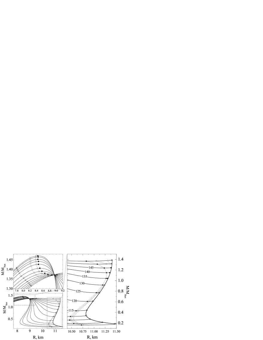
Fig. 3: Mass–radius $(M{-}R)$ relation for hybrid stars at $S_{\mathrm{k}}=0$. Each curve corresponds to its own equation of state for the quark phase. The values of the bag constant B are indicated by the numbers (in units of $\mbox{MeV}\cdot\mbox{fm}^{-3}$) near several curves. The bottom right panel shows a general view of the $(M{-}R)$ plane; the top left and right panels show magnified fragments. For the remaining explanations see the text.

An example of the calculation for the first case is shown in Fig. 3. The solid curves in this figure indicate the mass–radius $(M{-}R)$ relations for hybrid stars. Each curve corresponds to its own equation of state for the quark phase (the equations of state for the hadronic phase are identical). The values of the bag constant $B$ are indicated by the numbers (in units of $\mbox{MeV}\cdot\mbox{fm}^{-3}$) near several curves. The bottom left panel shows a general view of the $(M{-}R)$, plane; the top left and right panels show magnified fragments. Moving along the curve from right to left corresponds to an increase in the central density of the star. At the instant a new phase appears at the stellar center, the mass–radius curve abruptly (almost horizontally) goes to the left of the common envelope representing the $(M{-}R)$ relation for purely hadronic matter. Different densities at which quarks appear correspond to different values of the parameter $B$; the greater the value of $B$, the higher the density at which quark matter appears. Such a hybrid star initially becomes unstable until the core of the new phase becomes large enough and until the mass–radius curve passes through the minimum marked by the filled square. The stable branches of hybrid stars begin from the points of minimum, which reach the maximum while passing through the ‘‘singular point’’ (i.e., the place of intersection of the ‘‘bundle’’ of $(M{-}R)$ curves corresponding to different $B$; for an explanation of this peculiarity, see Yudin et al. 2014). These maxima correspond to the last stable configurations of hybrid stars (the black filled squares in the upper left part of Fig. 3). As the density at the stellar center increases further, there are no other stable configurations, and the star inevitably collapses into a black hole.

Let us now consider how the variational principle works in this situation. To begin with, we will take the first, ‘‘classical’’ function from our set $g_{1}=\upsilon$. For it the boundaries of the regions separating the stable and unstable models are indicated by the empty stars. Since this function is continuous at the PT, the variational principle for it contains only the integral term. The VP with this function completely ‘‘misses’’ the first instability zone shown on an enlarged scale in the right part of the figure corresponding to the region between the solid filled squares. However, the VP with this trial function shows the onset of instability with a noticeable delay (the stars in the upper left part of the figure) in the region of high densities as well. For the model of a star composed of purely hadronic matter, i.e., without any PT, this trial function predicts the onset of instability with a remarkable accuracy: the relative errors in the mass and radius are $\sim 0.01$ and $0.04\%$, respectively.

Let us now consider the VP with two functions (open circles) and with the complete set of three functions (triangles) in Fig. 3. As can be seen, the result has improved significantly, the first instability zone is now resolved, the instability zone beyond the maxima of the $(M{-}R)$ curves is also considerably closer to reality, with the results for the complete set of functions being much better than those for the set with two functions. The almost horizontal segments of the mass–radius curves, i.e., the regions in close proximity to the smooth extrema of the curves, are the only noticeable discrepancy. This is quite natural: the almost horizontal segment corresponds to an indifferent (or nearly indifferent) stellar equilibrium with respect to perturbations. The border between stability and instability here is very thin. Thus, we have shown that the VP with the basis functions of the specified form is actually capable of predicting the stability/instability of hybrid stars with a good accuracy. However, we would like to recall that this calculation is only an example.

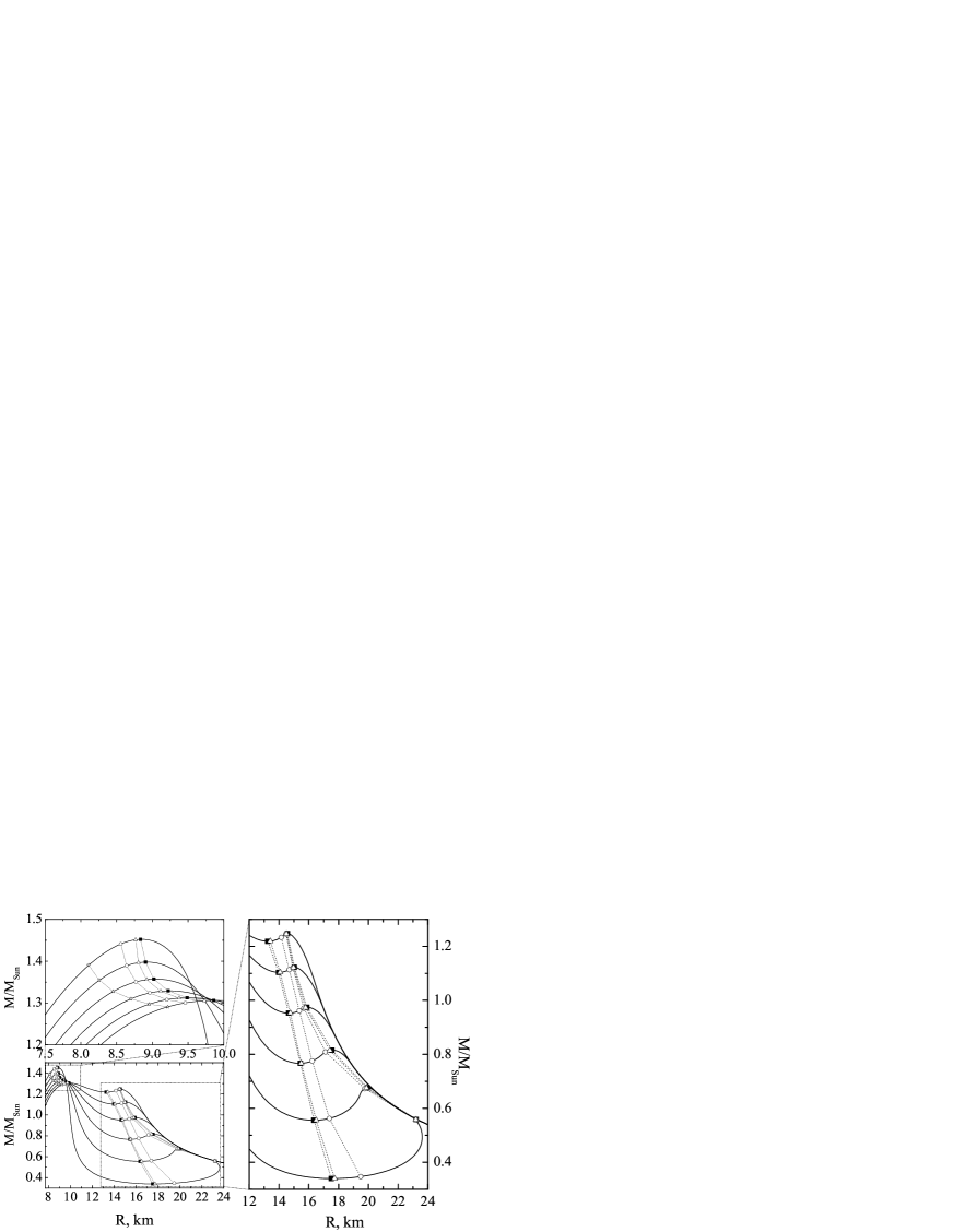
Fig. 4: Same as Fig. 3 for $S_{\mathrm{k}}=2$.

Let us now turn to the second case. Here, we consider hot isentropic stellar configurations with dimensionless entropy $S_{\mathrm{k}}=2$. The results are shown in Fig. 4, where the designations are the same as those in Fig. 3. Recall that the VP here works without the term outside the integral. As can be seen, the situation is generally similar to the previously considered case: the VP with one ‘‘classical’’ trial function completely misses the first instability zone at relatively low densities and shows the second one with a noticeable delay. Note that the situation with the stability when a new phase appears here is different from the case of $S_{\mathrm{k}}=0$: now the stability of a hybrid stellar configuration is lost only when the core of the new phase will grow to some size rather than immediately when it appears. On the whole, however, the results of the work of the VP with two and especially three basis functions are very close to the correct description of the stability.

CONCLUSIONS

Let us summarize what has been done in this paper. We began with the variational principle for stars with a phase transition that was first obtained by Bisnovatyi-Kogan et al. (1975). First we demonstrated that the well-known criterion for the onset of dynamical instability at PT at the stellar center $\lambda>3/2$ directly follows from it. We then showed that the term outside the integral of the VP naturally arises from the ordinary integral of the variational principle when using trial functions linear in mixing parameter in the region of mixed states. These results were then generalized to the relativistic case, with the form of the term outside the integral in GR having been obtained for the first time. Here, we obtained the generalization of the criterion $\lambda>3/2$ to the case of GR first found by Seidov (1971) by a different method directly from the VP.

As a demonstration of the fruitfulness of using the variational principle, we considered the problem of weak splitting of one PT into two smaller PTs and showed that such splitting increases the stability margin for the star. It would be also interesting to investigate the case of arbitrarily strong splitting. We are planning to do this in the immediate future.

Finally, we numerically studied the stability of hybrid stars within the framework of Newtonian gravity and in GR. First, we showed that using one ‘‘classical’’ basis function $\delta r\propto r$ is quite insufficient to describe the stability of stars with PT (although without PT it works excellently in both nonrelativistic and relativistic cases). Our natural desire would then be to restrict ourselves to a set of two basis functions the second of which would belong to the class of functions linear in mixing parameter in the region of mixed states that we found. However, it turned out that only three basis functions, two of which belong to the above-mentioned class, describe well the stability of hybrid stars. Since, as has already been said, each basis function multiplied by a smooth function that does not become zero at the stellar center can also serve as a basis one, we cannot be sure that we actually found the minimal set. We only demonstrated the fundamental efficiency of the variational principle in the case of hybrid stars. The problem of searching for the minimal set of basis functions and their optimal form requires an additional study.

REFERENCES

1. G.S. Bisnovatyi-Kogan, Astrophysics 4, 79 (1968).
2. G.S. Bisnovatyi-Kogan, Physical Questions of the Theory of Stellar Evolution, (Nauka, Moscow, 1989) [in Russian].
3. G.S. Bisnovatyi-Kogan, S.I. Blinnikov, and E.E. Shnol’, Sov. Astron. 19, 559 (1976).
4. B. Harrison, K. Thorne, M. Wakano, and J. Wheeler, Gravitation Theory and Gravitational Collapse, (Univ. Chicago Press, Chicago, 1965).
5. M.I. Krivoruchenko, D.K. Nadyozhin, T.L. Razinkova, Yu.A. Simonov, M.A. Trusov, A.V. Yudin, Phys. At. Nucl. 74, 371 (2011).
6. M.J. Lighthill, Mon. Not. R. Astron. Soc. 110, 339 (1950).
7. Z.F. Seidov, Sov. Astron. 15, 347 (1971).
8. A.V. Yudin, T.L. Razinkova, and D.K. Nadyozhin, Astron. Lett. 39, 161 (2013).
9. A.V. Yudin, T.L. Razinkova, D.K. Nadyozhin, and A.D. Dolgov, Astron. Lett. 40, 201 (2014).
10. Ya.B. Zel’dovich and I.D. Novikov, Relativistic Astrophysics, (Nauka, Moscow, 1967; Univ. Chicago Press, Chicago, 1971).