de Haas-van Alphen oscillations with non-parabolic dispersions

Abstract

de Haas-van Alphen oscillation spectrum of two-dimensional systems is studied for general power law energy dispersion, yielding a Fermi surface area of the form $S(E)\propto E^{\alpha}$ for a given energy $E$. The case $\alpha=1$ stands for the parabolic energy dispersion. It is demonstrated that the periodicity of the magnetic oscillations in inverse field can depend notably on the temperature. We evaluated analytically the Fourier spectrum of these oscillations to evidence the frequency shift and smearing of the main peak structure as the temperature increases.

1 Introduction

Due to their parabolic energy dispersion, most metallic systems, including organic conductors, heavy fermions, give way to de Haas-van Alphen (dHvA) oscillations periodic in inverse magnetic field $B$, with a periodicity proportional to the Fermi surface area supporting the cyclotronic trajectory of the quasiparticle. When only one band is involved, the Fourier spectrum is composed of a series of peaks with a fundamental frequency and its harmonics. The precise amplitude of these peaks is given by the Lifshitz-Kosevich (LK) formula [1, 2, 3, 4, 5], originally derived for three dimensional metals with parabolic band structures (for which the Fermi surface area grows or decreases linearly with energy). It also holds for strongly two-dimensional band structures where metallic layers are separated from each other by insulating layers, as it is the case of the organic metals $\theta$-(ET)₄CoBr₄(C₆H₄Cl₂) [6] or $\theta$-(ET)₄ZnBr₄(C₆H₄Cl₂) [7], albeit oscillation of the chemical potential in magnetic field must be taken into account for these non-compensated metals.

In contrast, deviation to parabolic energy dispersion, namely in presence of a curvature $S^{\prime\prime}(E)\neq 0$ when the Fermi surface area grows non-linearly with the energy, leads to an additional Onsager phase in the oscillations that is dependent on the magnetic field $B$ and the temperature $T$. In the limit where the ratio $B/T$ is either large or small, this phase is proportional to $T^{2}/B$  [8], which yields, in the considered field ranges, a temperature dependent frequency. Notably, this behavior should be observed in the case of Dirac fermions, the energy dispersion of which is linear with the momentum [9] and liable to yield non-parabolic deviations. Indeed, the energy curvature of the Fermi surface area is proportional in this case to $S^{\prime\prime}(E)=2\pi/(hv_{F})^{2}$ where $v_{F}\simeq 10^{6}$m/s is the Fermi velocity.

It must be pointed out that the observed frequency changes and (or) phase shifts of the oscillations can also be attributed to other physical effects which have to be treated separately. For example, spin-orbit coupling leads to a splitting of the Fermi surface, hence of the dHvA frequency with a magnitude proportional to $B^{2}$ and to the effective mass [10]. Such splitting has been considered in data relevant to e.g. bilayer underdoped high-T_c cuprates [11]. Phase shift is observed in the presence of magnetic breakdown when the Fermi surface is composed of several bands between which the quasiparticles can tunnel, leading to giant orbits. In this case, the field-dependent phase is linked to the probability of tunneling [12, 13, 14]. It depends on the ratio between the breakdown field and the field itself, but not the temperature. Its origin comes from a linearization of the Fermi surface near the tunneling region for which the quantum wavefunctions can be solved. This problem is similar to the Zener effect [15] but in a magnetic field. Such phase has been observed and studied in the organic compound $\theta$-(BEDT-TTF)₄CoBr₄(C₆H₄Cl₂) where the breakdown field is close to 35 T [16]. To end with examples, strong deviation from parabolicity is observed within the tight-binding model in two dimensions where the band gap closes at half-filling, yielding non LK behavior of the oscillation amplitude [17].

In this paper, we focus on special cases of power law spectrum dependence of the Fermi surface area $S(E)\propto E^{\alpha}>0$, where the exponent $\alpha$ is taken as a control parameter, either negative or positive, standing respectively for hole or electron-type quasiparticles. In section 2, magnetization is evaluated from an exact resummation of the grand potential in the quasi-classical limit of small fields, and the result is given by Eq. (6), which is a general formula from which dHvA oscillations can be analyzed. In section 3, we apply our analysis to power law dispersion, where exact integrals can be performed. Both cases $\alpha<0$ and $\alpha>0$ are studied and the peak structure of the temperature-dependent Fourier transform is discussed. In particular, calculations are made for $\alpha<0$ and $\alpha\geq 1$, relevant to hole-type quasiparticles and electron-type Dirac fermions, respectively. In the last section 4, we provide a low-temperature expression of magnetization in the general case.

2 Expansion of the grand potential

Let us consider a band structure in a two-dimensional system, yielding a closed surface area in the Brillouin zone equal to $S(E)=\oint_{E}k_{y}\mathrm{d}k_{x}/4\pi^{2}$ at constant energy $E$. In the parabolic case $S(E)=E$ and for Dirac fermions $S(E)=E^{2}$. The quantization of Landau levels is given by the Bohr-Sommerfeld rule $S(E_{n})=b(n+\gamma)$, with the reduced field $b=eB/h$ in inverse area units where $-e$ is the electron charge. Indeed, for typical elementary cell areas, $b$ is small and a semi-classical analysis can be applied. We want to study in the next section 3 the oscillations of the magnetization for the class of surfaces with a power law dependence $S(E)=E^{\alpha}$, where $\alpha=1$ stands for a parabolic surface.

To be more rigorous with the units, we should consider the physical coefficient of proportionality $k_{\alpha}$ between $S(E)$ and $E^{\alpha}$ (with units $[k_{\alpha}]=L^{-2}E^{-\alpha}$ where $L$ is a length and $E$ an energy) but for simplicity we will ignore it. It can be restored at the end of the computations by rescaling $b\rightarrow b/k_{\alpha}$ (with $[b]=L^{-2}$ and $[b/k_{\alpha}]=E^{\alpha}$), and frequency $F\rightarrow F/k_{\alpha}$ (with $[F]=L^{-2}$ and $[F/k_{\alpha}]=E^{\alpha}$) accordingly. For example, the surface areas for the free fermions and Dirac fermions in real units are respectively given by

$$S(E)=m^{*}E/(2\pi\hbar^{2}),\;S(E)=\pi E^{2}/(2\pi\hbar v_{F})^{2}$$ (1)

where $m^{*}$ is the effective mass of the quasiparticle. The temperature $T$ will be expressed in units of $\mu/k_{B}$ in the numerical applications further below, where $\mu$ is the chemical potential. More specifically, the fundamental frequency $F_{0}$ of the oscillation spectrum is equal to $F_{0}=hS(\mu)/e=(h/e)k_{\alpha}\mu^{\alpha}$ in Tesla, since $h/e$ is a quantum flux and $S(\mu)$ is the area of the cyclotronic trajectory in the Brillouin zone (inverse square length). The reduced temperature $t$ can then be expressed as $t=k_{B}T/\mu=k_{B}(k_{\alpha}h/e)^{1/\alpha}T/F_{0}^{1/\alpha}$, with $T$ expressed in Kelvin and $F_{0}$ in Tesla. For $\alpha=1$, one finds that $t=0.745T(m^{*}/m_{e})/F_{0}$, and when $\alpha=2$, one has instead $t=2375.2T/(v_{F}F_{0}^{1/2})$.

In this section, we will give the expression of the oscillatory part of the grand potential in the more general case, not restricted to the power law class, and the main result is given by Eq. (6). We first consider the oscillating part of the grand potential obtained from the Poisson formula for an arbitrary discrete Landau spectrum [18]

$$\frac{\Omega_{osc}}{A}= -\frac{2b}{\beta}{\rm Re}\sum_{p=1}^{\infty}\int_{0}^{\infty}\mathrm{d}n\log\left[1+{\rm e}^{\beta(\mu-E_{n})}\right]{\rm e}^{2i\pi pn}$$

$$= -\frac{2b}{\beta}{\rm Re}\sum_{p=1}^{\infty}I_{p}$$ (2)

where $\beta=(k_{B}T)^{-1}$ and $A$ is the sample area. Following the analysis leading to the LK result, we perform an integration by parts of the partial quantities $I_{p}$

$$I_{p}= -\frac{1}{2i\pi p}\log[1+{\rm e}^{\beta(\mu-E_{0})}]-\frac{\beta}{(2i\pi p)^{2}}E_{0}^{\prime}\phi_{0}$$

$$+\frac{\beta^{2}}{(2i\pi p)^{2}}\int_{0}^{\infty}\mathrm{d}n{\rm e}^{2i\pi pn}E_{n}^{\prime 2}\phi_{n}^{\prime}-\frac{\beta}{(2i\pi p)^{2}}\int_{0}^{\infty}\mathrm{d}n{\rm e}^{2i\pi pn}E_{n}^{\prime\prime}\phi_{n}$$ (3)

where we have defined $\phi_{n}=\phi(\beta[\mu-E_{n}])$ and $\phi(x)=(1+{\rm e}^{-x})^{-1}$. In the LK theory, i.e. for a parabolic band, the last term is zero since $E_{n}^{\prime\prime}=0$. And the function $\beta\phi_{n}^{\prime}$ behaves like a Dirac distribution in the low temperature limit around the Fermi energy . The LK approximation is relying on computing this integral in the complex plane in the low temperature limit when $-\beta\mu\rightarrow-\infty$, after a change of variable $n(E)\rightarrow E$ is performed. The poles of the function $\phi^{\prime}$ considered for applying the residue theorem are located on the upper plane. After performing a resummation over the poles as a geometrical series, one obtains an expression for the thermal amplitude that decays exponentially with the temperature. The first term on the right hand side of Eq. (3) is a pure imaginary number, and despite the divergence of the sum over $p$, it does not contribute to the real part of $I_{p}$ and can be discarded in the following. In the general non-parabolic case, we can perform an additional integration by parts on the last term in order to single out the function $\beta\phi_{n}^{\prime}$

$$I_{p}= -\frac{\beta}{(2i\pi p)^{2}}E_{0}^{\prime}\phi_{0}+\frac{\beta}{(2i\pi p)^{3}}E_{0}^{\prime\prime}\phi_{0}+\frac{\beta^{2}}{(2i\pi p)^{2}}\int_{0}^{\infty}\mathrm{d}n{\rm e}^{2i\pi pn}E_{n}^{\prime 2}\phi_{n}^{\prime}$$

$$- \frac{\beta^{2}}{(2i\pi p)^{3}}\int_{0}^{\infty}\mathrm{d}n{\rm e}^{2i\pi pn}E_{n}^{\prime}E_{n}^{\prime\prime}\phi_{n}^{\prime}+\frac{\beta}{(2i\pi p)^{3}}\int_{0}^{\infty}\mathrm{d}n{\rm e}^{2i\pi pn}E_{n}^{\prime\prime\prime}\phi_{n}$$ (4)

The last integral whose integrand is proportional to $\phi_{n}$ can be furthermore integrated by parts, and this process can be repeated indefinitely. One obtains a formal series as the result of all the consecutive partial integrations which is expressed as

$$I_{p}= \beta\sum_{k=1}^{\infty}\frac{(-1)^{k}}{(2i\pi p)^{k+1}}E_{0}^{(k)}\phi_{0}+\beta^{2}\int_{0}^{\infty}\mathrm{d}n{\rm e}^{2i\pi pn}E_{n}^{\prime}\phi_{n}^{\prime}\sum_{k=1}^{\infty}\frac{(-1)^{k+1}}{(2i\pi p)^{k+1}}E_{n}^{(k)}$$ (5)

This series can be resummed and put into a single integral using the formula $\sum_{k=0}^{\infty}(-x)^{k}f^{(k)}(n)=\int_{0}^{\infty}\mathrm{d}u{\rm e}^{-u}f(n-ux)$. One easily obtains a compact form for the partial quantities $I_{p}$ as the sum of two terms

$$I_{p}= \frac{\beta\phi_{0}}{2i\pi p}\int_{0}^{\infty}\mathrm{d}u{\rm e}^{-u}\left[E_{-u/(2i\pi p)}-E_{0}\right]$$

$$-\frac{\beta^{2}}{2i\pi p} \int_{0}^{\infty}\mathrm{d}n{\rm e}^{2i\pi pn}E_{n}^{\prime}\phi_{n}^{\prime}\int_{0}^{\infty}\mathrm{d}u{\rm e}^{-u}\left[E_{n-u/(2i\pi p)}-E_{n}\right]$$ (6)

This expression encompasses all the deviations from parabolicity without linearization and is the main formula of this work from which we can deduce physical implications of any specific dispersion $E_{n}$ on the dHvA oscillatory Fourier spectrum. The simplest example is provided by the parabolic dispersion, $E_{n}=b(n+\gamma)$ with $\gamma=1/2$, for which the integral over $u$ in Eq. (6) can be easily performed. In this case, it is convenient to change the variable $n\rightarrow n(E)=E/b-\gamma$ to obtain

$$I_{p}=-\frac{\beta b\phi_{0}}{(2i\pi p)^{2}}+\frac{\beta^{2}b}{(2i\pi p)^{2}}\int_{0}^{\infty}\mathrm{d}E{\rm e}^{2i\pi p(E/b-\gamma)}\phi^{\prime}(\beta[\mu-E])$$

Then the integral of the previous expression can be computed after the rescaling of the energy $2\pi x=\beta(E-\mu)$

$$\int_{0}^{\infty}\mathrm{d}E{\rm e}^{2i\pi p(E/b-\gamma)}\phi^{\prime}(\beta[\mu-E])={\rm e}^{2i\pi p\mu/b-2i\pi p\gamma}\int_{-\beta\mu/2\pi}^{\infty}\frac{\pi\mathrm{d}x}{2\beta}\frac{{\rm e}^{4i\pi^{2}px/(\beta b)}}{\cosh^{2}(\pi x)}$$ (7)

At low temperature, it is usual to replace the lower bound $-\beta\mu/2\pi$ by $-\infty$. Then the residue theorem can be applied in the upper plane, where the zeroes of function $\cosh(\pi x)$, which are the poles of the integrand, are given by $x_{n}=i(n+1/2)$, $n\geq 0$. After the resummation over the $x_{n}$, one obtains a temperature dependent damping amplitude $R$ defined by

$$\int_{-\infty}^{\infty}\frac{\pi\mathrm{d}x}{2}\frac{{\rm e}^{4i\pi^{2}px/(\beta b)}}{\cosh^{2}(\pi x)}=R\left(\frac{2\pi^{2}p}{\beta b}\right),\;R(x)=\frac{x}{\sinh(x)}$$ (8)

Then, the dominant part of the grand potential is given by

$$\frac{\Omega_{osc}}{A}\simeq\sum_{p=1}^{\infty}\frac{b^{2}}{2\pi^{2}p^{2}}R\left(\frac{2\pi^{2}p}{\beta b}\right)\cos\left(2\pi p\frac{\mu}{b}-2\pi p\gamma\right)$$ (9)

The oscillating part of the magnetization is defined by $m_{osc}=-A^{-1}\partial\Omega_{osc}/\partial b$, or, with a good approximation

$$m_{osc}(b)\simeq-\sum_{p=1}^{\infty}\frac{\mu}{\pi p}R\left(\frac{2\pi^{2}p}{\beta b}\right)\sin\left(2\pi p\frac{\mu}{b}-2\pi p\gamma\right)$$ (10)

which is the LK formula. After restoring the correct units $b\rightarrow b/k_{1}=2\pi\hbar^{2}b/m^{*}=\hbar\omega_{c}$, with cyclotron frequency $\omega_{c}=eB/m^{*}$, one finds that the fundamental frequency is equal to $F_{0}=m^{*}\mu/(\hbar e)$. Now the thermal damping amplitude $R$ is usually written as $R(2\pi^{2}pk_{B}T/\hbar\omega_{c})=R(u_{0}(m^{*}/m_{e})pT/B)$, with $u_{0}=2\pi^{2}k_{B}m_{e}/\hbar e=14.7$ T/K for an electron of mass $m_{e}$. This thermal factor is essential in determining the quasi-particle mass $m^{*}$ from the temperature dependence of the Fourier amplitude of each harmonic $pF_{0}$.

3 Surfaces with a power law dependence

In this section we consider the general case of a power law dependence of the area $S(E)=E^{\alpha}$. When $\alpha$ is negative the surface is a hole-type surface, with a negative geometrical mass $S^{\prime}(E)<0$, whereas when $\alpha>0$ the surface is an electronic band with a positive mass. Eq. (6) can be rewritten, after discarding the first term which is assumed to be small, as

$$I_{p}= -\frac{\beta^{2}}{2i\pi p}\int_{0}^{\infty}\mathrm{d}EE{\rm e}^{2i\pi p(E^{\alpha}/b-\gamma)}\phi^{\prime}(\beta[\mu-E])$$

$$\times \int_{0}^{\infty}\mathrm{d}u{\rm e}^{-u}\left[\left(1-\frac{bu}{2i\pi pE^{\alpha}}\right)^{1/\alpha}-1\right]$$ (11)

Magnetization, defined by $m_{osc}=-A^{-1}\partial\Omega_{osc}/\partial b$, is dominated by the derivative of the exponential phase ${\rm e}^{2i\pi pE^{\alpha}/b}$, which gives a main contribution in $1/b^{2}$, and after a change of variable $bu/pE^{\alpha}\rightarrow u$, one obtains the expression

$$m_{osc}(b)\simeq\frac{2}{b^{2}}{\rm Re}\sum_{p\geq 1}p{\rm e}^{-2i\pi p\gamma}\int_{0}^{\infty}\mathrm{d}EE^{1+2\alpha}{\rm e}^{2i\pi pE^{\alpha}/b}$$

$$\times\beta\phi^{\prime}(\beta[\mu-E])\int_{0}^{\infty}\mathrm{d}u{\rm e}^{-pE^{\alpha}u/b}\left[\left(1-\frac{u}{2i\pi}\right)^{1/\alpha}-1\right]$$ (12)

In the parabolic case $\alpha=1$, one easily finds

$$m_{osc}(b)\simeq-2{\rm Re}\sum_{p\geq 1}\frac{1}{2i\pi p}\int_{0}^{\infty}\mathrm{d}EE{\rm e}^{2i\pi p(E/b-\gamma)}\beta\phi^{\prime}(\beta[\mu-E])$$ (13)

We want to study the general Fourier spectrum $A(F)$ of the magnetization with respect to the inverse field $x=1/b$, where $x$ is taken by extension from $-\infty$ to $+\infty$, and from which $m_{osc}(b)={\rm Re}\int_{-\infty}^{\infty}\mathrm{d}FA(F){\rm e}^{2i\pi F/b}$. In the parabolic case the amplitude can be computed exactly since the integral over $x$ involves only a Dirac function

$$A(F)= -\sum_{p\geq 1}\frac{1}{i\pi p}\int_{-\infty}^{\infty}\mathrm{d}x\int_{0}^{\infty}\mathrm{d}EE{\rm e}^{2i\pi(pE-F)x-2i\pi p\gamma}\beta\phi^{\prime}(\beta[\mu-E])$$

$$= -2F\sum_{p\geq 1}\frac{e^{-2i\pi p\gamma}}{2i\pi p^{3}}\beta\phi^{\prime}(\beta[\mu-F/p])\theta(F)$$ (14)

Here $\theta$ is the Heaviside function. The amplitude $A(F)$ is peaked at frequencies $F=p\mu$ as expected. $A(F)$ is purely imaginary in the case where $\gamma=1/2$. In the LK theory, the factor $F$ in front of Eq. (14) is replaced by the saddle point solution $p\mu$.

3.1 Hole-type quasiparticles ($\alpha<0$)

In this section, we focus on the case $\alpha<0$ with the aim to evaluate the Fourier transform of the magnetization Eq. (12). It is useful to consider the following formula representation of the last integral over $u$ in Eq. (12) when $\alpha<0$ for complex $z$ with positive real and imaginary parts

$$\int_{0}^{\infty}\mathrm{d}u{\rm e}^{-zu}\left[(1-\frac{u}{2i\pi})^{1/\alpha}-1\right]= -z^{-1}-2i\pi{\rm e}^{-2i\pi z}\int_{1}^{\infty}\mathrm{d}uu^{1/\alpha}{\rm e}^{2i\pi zu}$$

$$= -z^{-1}-2i\pi{\rm e}^{-2i\pi z}E_{-1/\alpha}(-2i\pi z)$$ (15)

where $E_{n}(z)=\int_{1}^{\infty}\mathrm{d}uu^{-n}{\rm e}^{-zu}$ are the exponential integral. This representation is only valid for $\alpha<0$ otherwise the integral on the right hand side would diverge at large argument. Magnetization can then be written as

$$m_{osc}(b)= -\frac{2}{b}{\rm Re}\sum_{p\geq 1}{\rm e}^{-2i\pi p\gamma}\int_{0}^{\infty}\mathrm{d}EE^{1+\alpha}\beta\phi^{\prime}(\beta[\mu-E])$$

$$\times\left[{\rm e}^{2i\pi pE^{\alpha}/b}+\frac{2i\pi pE^{\alpha}}{b}\int_{1}^{\infty}\mathrm{d}uu^{1/\alpha}{\rm e}^{2i\pi pE^{\alpha}u/b}\right]$$

$$= -\frac{2}{b}{\rm Re}\sum_{p\geq 1}{\rm e}^{-2i\pi p\gamma}\int_{0}^{\infty}\mathrm{d}EE^{1+\alpha}\beta\phi^{\prime}(\beta[\mu-E])$$ (16)

$$\times\left[{\rm e}^{2i\pi pE^{\alpha}/b}+\frac{2i\pi pE^{\alpha}}{b}E_{-1/\alpha}(-2i\pi pE^{\alpha}/b)\right]$$

The integral over $E$ is convergent near the origin only if $-1<\alpha<0$ due to the presence of a term proportional to $E^{1+2\alpha}$ in the expression. Otherwise a cut-off should be introduced when $E$ is small, for which the Fermi surface area $S(E)$ diverges strongly. The Fourier amplitude $A(F)$ can now be evaluated from Eq. (16) after performing different integrations over the variables $x=1/b$ and $u$ respectively

$$A(F)=\frac{i}{\pi\alpha}\frac{\partial}{\partial F}\sum_{p\geq 1}\frac{{\rm e}^{-2i\pi p\gamma}}{p^{1/\alpha}}F^{1/\alpha-1}\int_{(F/p)^{1/\alpha}}^{\infty}\mathrm{d}EE^{\alpha}\beta\phi^{\prime}(\beta[\mu-E])\theta(F)$$ (17)

$A(F)$ is a pure imaginary number when $\gamma=1/2$ or $\gamma=0$. We have plotted the imaginary part $-\Im A(F)$ in Fig. 1(b), for several values of temperatures, and compared it with the parabolic case Fig. 1(a) from Eq. (14). The dominant peak structure is centered at harmonics $F=p/\mu$ but, contrary to the parabolic case, the peaks are moving to lower values as the temperature increases. In the parabolic case the deviation is present although less pronounced. It is due to the presence of the factor $F$ in front of Eq. (14), which is considered as constant and equal to $\mu$ in the LK theory. But the deviation is too small to be observed at temperatures where the amplitude is not negligibly small. In any case, this approximation is valid for the temperature range explored in experiments. In short, as the temperature increases, the frequency of the Fourier components decreases and increases, for electron and hole type quasiparticles, respectively, the frequency variation being more pronounced for hole type quasiparticles.

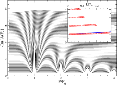
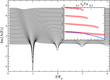
(a) (b)

Figure 1: Plot of the Fourier amplitude $-\Im\{A(F)\}$ for the cases $\alpha=1$ (a) and $\alpha=-1$ (b), respectively, and for temperatures ranging from t=0.01 up to t=0.3, where $t=k_{B}T/\mu$. Here we have taken $\gamma=0$ in both cases for simplicity, otherwise the peaks take alternative signs. In the insets is represented the temperature dependence of the extrema. For electron-type particles, the peaks are moving to the right as the temperature increases, whereas for hole-type they move to the opposite direction. Solid blue lines are the low temperature approximation of the first harmonics given by Eq. (27). Curves are obtained from the numerical resolution of Eq. (22) and Eq. (17) respectively, and the positions of the extrema are found numerically.

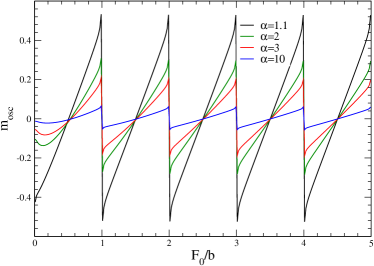
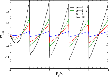
(a) (b)

Figure 2: Plot of the magnetization at zero temperature for different values of $\alpha$ as a function of the inverse field $F_{0}/b$.

3.2 Electron-type quasiparticles ($\alpha>1$)

In this section, we consider the Fourier amplitude of Eq. (12) when $\alpha\geq 1$. For other cases $0<\alpha<1$ the techniques developed below can be applied as well with some modifications. We would like to get a representation of the last integral on the right hand side of Eq. (12) still in terms of exponential integrals such as in Eq. (15). Indeed, the exponential integral on the right hand side of Eq. (15) is not finite for imaginary argument and $\alpha>0$ as seen before. However we can use a differentiation

$$\int_{0}^{\infty}\mathrm{d}u{\rm e}^{-zu}\left(1-\frac{u}{2i\pi}\right)^{1/\alpha}=\frac{{\rm e}^{-2i\pi z}}{2i\pi}\frac{\partial}{\partial z}\left[\int_{0}^{\infty}\mathrm{d}u{\rm e}^{-z(u-2i\pi)}\left(1-\frac{u}{2i\pi}\right)^{1/\alpha-1}\right]$$ (18)

Since $1/\alpha-1$ is negative for $\alpha>1$, we can apply Eq. (15) to have a useful representation for the integral after the differentiation operator. In particular, we can write the last integral of Eq. (12) as

$$\int_{0}^{\infty}\mathrm{d}u{\rm e}^{-pE^{\alpha}u/b}\left(1-\frac{u}{2i\pi}\right)^{1/\alpha}= \frac{b{\rm e}^{-2i\pi pE^{\alpha}/b}}{2i\pi pE^{\alpha}}\frac{\partial}{\partial\lambda}\int_{0}^{\infty}\mathrm{d}u{\rm e}^{-pE^{\alpha}(u-2i\pi)/b}\left(1-\frac{u}{2i\pi}\right)^{1/\alpha-1}\Big{|}_{\lambda=1}$$

$$= -\frac{b{\rm e}^{-2i\pi pE^{\alpha}/b}}{pE^{\alpha}}\frac{\partial}{\partial\lambda}\int_{1}^{\infty}\frac{\mathrm{d}u}{u^{1-1/\alpha}}{\rm e}^{2i\pi pE^{\alpha}\lambda u/b}\Big{|}_{\lambda=1}$$

$$= -\frac{b{\rm e}^{-2i\pi pE^{\alpha}/b}}{pE^{\alpha}}\frac{\partial}{\partial\lambda}\int_{\lambda}^{\infty}\frac{\lambda^{-1/\alpha}\mathrm{d}u}{u^{1-1/\alpha}}{\rm e}^{2i\pi pE^{\alpha}u/b}\Big{|}_{\lambda=1}$$

$$= \frac{b{\rm e}^{-2i\pi pE^{\alpha}/b}}{pE^{\alpha}}\left[{\rm e}^{2i\pi pE^{\alpha}/b}+\frac{1}{\alpha}\int_{1}^{\infty}\frac{\mathrm{d}u}{u^{1-1/\alpha}}{\rm e}^{2i\pi pE^{\alpha}u/b}\right]$$ (19)

From this representation, one can express the magnetization as

$$m_{osc}(b)= \frac{2}{\alpha b}{\rm Re}\sum_{p\geq 1}{\rm e}^{-2i\pi p\gamma}\int_{0}^{\infty}\mathrm{d}EE^{1+\alpha}\beta\phi^{\prime}(\beta[\mu-E])\int_{1}^{\infty}\frac{\mathrm{d}u{\rm e}^{2i\pi pE^{\alpha}u/b}}{u^{1-1/\alpha}}$$ (20)

Then we can write the Fourier amplitude of Eq. (12) as

$$A(F)= \frac{2}{\alpha}\sum_{p\geq 1}\int_{-\infty}^{\infty}\mathrm{d}xx{\rm e}^{-2i\pi p\gamma-2i\pi Fx}\int_{0}^{\infty}\mathrm{d}EE^{1+\alpha}\beta\phi^{\prime}(\beta[\mu-E])\int_{1}^{\infty}\frac{\mathrm{d}u{\rm e}^{2i\pi pE^{\alpha}ux}}{u^{1-1/\alpha}}$$

$$= \frac{i}{\pi\alpha}\frac{\partial}{\partial F}\sum_{p\geq 1}{\rm e}^{-2i\pi p\gamma}\int_{0}^{\infty}\mathrm{d}EE^{1+\alpha}\beta\phi^{\prime}(\beta[\mu-E])\int_{1}^{\infty}\frac{\mathrm{d}u}{u^{1-1/\alpha}}\delta(F-pE^{\alpha}u)$$ (21)

After integration over $u$ one finally obtains the simple expression

$$A(F)= \frac{i}{\pi\alpha}\frac{\partial}{\partial F}\sum_{p\geq 1}\frac{{\rm e}^{-2i\pi p\gamma}}{p^{1/\alpha}}F^{1/\alpha-1}\int_{0}^{(F/p)^{1/\alpha}}\mathrm{d}EE^{\alpha}\beta\phi^{\prime}(\beta[\mu-E])\theta(F)$$ (22)

This expression is the same as Eq. (17) except for the interval integration. We recover in particular the result Eq. (14) in the parabolic case $\alpha=1$ by simple differentiation of the integral since the term $F^{1/\alpha-1}=1$. For Dirac fermions, $\alpha=2$ and $\gamma=0$, we can check the formula Eq. (22) with direct computation of the Fourier transform of Eq. (12):

$$A(F)= \frac{1+i}{2}\sum_{p\geq 1}\frac{1}{\sqrt{p}}\int_{0}^{\infty}\mathrm{d}EE^{2}\beta\phi^{\prime}(\beta[\mu-E])$$

$$\times \int_{-\infty}^{\infty}\mathrm{d}x\sqrt{x}{\rm e}^{-2i\pi Fx}{\rm erfc}\left(\sqrt{\pi pE^{2}x}(1-i)\right)$$ (23)

The integration over $x$ seems not easy to perform at first, but the erfc function is related to the integral function of argument $1/2$ by ${\rm erfc}(z)=z\pi^{-1/2}E_{1/2}(z^{2})$

$$A(F)= \sum_{p\geq 1}\int_{0}^{\infty}\mathrm{d}EE^{3}\beta\phi^{\prime}(\beta[\mu-E])\int_{-\infty}^{\infty}\mathrm{d}xx{\rm e}^{-2i\pi Fx}E_{-1/2}(-2i\pi pE^{2}x)$$ (24)

Then we use the integral representation of function $E_{1/2}$ which allows to perform the integration over $x$. This leads to the same result as Eq. (22) given by

$$A(F)= \frac{1}{4i\pi}\sum_{p\geq 1}\frac{\theta(F)}{\sqrt{p}}\Big{[}F^{-3/2}\int_{0}^{\sqrt{F/p}}\mathrm{d}EE^{2}\beta\phi^{\prime}(\beta[\mu-E])-p^{-3/2}\beta\phi^{\prime}(\beta[\mu-\sqrt{F/p}])\Big{]}$$ (25)

The amplitudes $A(F)$ in Eq. (17) and Eq. (22) are both pure imaginary, and the magnetization is given by $m_{osc}(b)=-\int_{0}^{\infty}\Im\{A(F)\}\sin(2\pi F/b)$. In Fig. 2 we have represented the magnetization for different values of $\alpha$, positive and negative respectively. As $\alpha$ increases, the amplitude of the oscillations decreases. This is due to the $\alpha$-dependence of the effective mass that we defined by

$$m^{*}=2\pi\hbar^{2}\partial S(\mu)/\partial\mu=2\pi\hbar^{2}k_{\alpha}\alpha\mu^{\alpha-1}$$ (26)

The ratio of the effective mass to the dominant frequency (in restored units of the square of inverse length) is directly proportional to $\alpha$, since $m^{*}/F_{0}=2\pi\hbar^{2}\alpha/\mu$, and the absolute value of $m^{*}$ ($m^{*}$ is negative in the case of $\alpha<0$) increases as $\alpha$ increases when $F_{0}$ is kept fixed. This accounts for the behavior of the oscillations reported in Fig. 2 whose amplitude become smaller as $\alpha$ increases. The maximum amplitude is obtained for the parabolic case.

3.3 Temperature dependence of the dominant frequency

Here we consider the low temperature limit of the previous expressions  Eq. (17) and Eq. (22), and evaluate the value of the dominant frequency for $p=1$. At zero temperature, this corresponds to $F_{0}=\mu^{\alpha}$, or to the first extremum of $A(F)$. We can perform an expansion around this value, by assuming the parameter $\Delta=(F^{1/\alpha}-\mu)/2T$ to be small, $\Delta=O(T)$, and extremizing the first harmonic term as function of $\Delta$. For both cases, $\alpha$ negative and positive, one finds the following expansion

$$F_{0}\simeq\mu^{\alpha}\left\{1+2\alpha(3-2\alpha)\frac{(k_{B}T)^{2}}{\mu^{2}}\right\}$$ (27)

The coefficient in front of $(T/\mu)^{2}$ is always negative for $\alpha<0$ and $\alpha>3/2$, and positive in the interval $0<\alpha<3/2$. This can be compared to the fundamental frequency $F_{0}$ deduced from the numerical resolutions of Eqs. 14 and 17 reported in the insets of Fig. 1, where solid blue lines are low temperature approximations given by  Eq. (27) for $\alpha=1$, with the slope $2\alpha(3-2\alpha)=2$, and $\alpha=-1$, with the slope $2\alpha(3-2\alpha)=-10$. Accordingly, the temperature dependence is steeper for $\alpha$=-1, while for $\alpha=(3-\sqrt{17})/4\simeq-0.28$ the slope ($-2$) is opposite to the one for the parabolic case.

4 Low temperature expansion

In this section, we consider the temperature behavior of the magnetization in the low temperature limit $\beta\gg 1$. It is useful to consider the Fourier transform of the function $\beta\phi^{\prime}$

$$\beta\phi^{\prime}(\beta[\mu-E])= \frac{\beta}{4\cosh^{2}\left(\makebox{\small$\frac{1}{2}$}\beta[E-\mu]\right)}=\beta\int_{-\infty}^{\infty}\frac{\mathrm{d}g}{2\pi}R(\pi g){\rm e}^{i\beta g(E-\mu)}$$ (28)

which is convenient for a stationary phase approximation since the phase $\beta gE$ of the exponential argument is large. Considering the case $\alpha>1$, the magnetization Eq. (20) includes a triple integral over $g$, $u$ and $E$

$$m_{osc}(b)= \frac{2}{\alpha b}{\rm Re}\sum_{p\geq 1}{\rm e}^{-2i\pi p\gamma}\int_{1}^{\infty}\frac{\mathrm{d}u}{u^{1-1/\alpha}}\int_{-\infty}^{\infty}\frac{\beta\mathrm{d}g}{2\pi}R(\pi g)$$

$$\times \int_{0}^{\infty}\mathrm{d}EE^{1+\alpha}{\rm e}^{2i\pi pE^{\alpha}u/b+ig\beta(\mu-E)}$$ (29)

We then apply the phase approximation to the argument function $\varphi(E,g)=2i\pi pE^{\alpha}u/b+ig\beta(\mu-E)$ for which the stationary solutions $\partial_{E}\varphi(E,g)=\partial_{g}\varphi(E,g)=0$ are given by $E^{*}=\mu$ and $g^{*}=2\pi p\alpha u\mu^{\alpha-1}/\beta b$. One obtains a temperature dependence of the magnetization in the general case as

$$m_{osc}(b)\simeq \frac{2\mu^{1+\alpha}}{\alpha b}{\rm Re}\sum_{p\geq 1}{\rm e}^{-2i\pi p\gamma}\int_{1}^{\infty}\frac{\mathrm{d}u}{u^{1-1/\alpha}}R\left(\frac{2\pi^{2}p\mu^{\alpha-1}u}{\beta b}\right){\rm e}^{2i\pi p\mu^{\alpha}u/b}$$ (30)

which is valid only for $\alpha>1$. For negative values of $\alpha<0$, the same analysis leads to the following approximation

$$m_{osc}(b)\simeq -\frac{2\mu^{1+\alpha}}{b}{\rm Re}\sum_{p\geq 1}{\rm e}^{-2i\pi p\gamma}\left[R\left(\frac{2\pi^{2}p\mu^{\alpha-1}}{\beta b}\right){\rm e}^{2i\pi p\mu^{\alpha}/b}\right.$$

$$\left.+\frac{2i\pi p\mu^{\alpha}}{b}\int_{1}^{\infty}\frac{\mathrm{d}u}{u^{-1/\alpha}}R\left(\frac{2\pi^{2}p\mu^{\alpha-1}u}{\beta b}\right){\rm e}^{2i\pi p\mu^{\alpha}u/b}\right].$$ (31)

The physical values of the temperature for which the oscillations can be seen are bounded by the limit $\hbar\omega_{c}=k_{B}T$, or $\beta b=1$ in the reduced units. This corresponds to the limit where the thermal energy is equal to the Landau gap.

5 Discussion and Conclusion

The dHvA Fourier spectrum was analyzed for a class of Fermi surfaces whose area grows like $E^{\alpha}$, by performing exact integrations of the oscillatory part of the grand potential harmonics. This is relevant in particular for Dirac spectrum for which $\alpha=2$. All the deviations from parabolicity in the LK theory, which consists in a linearization of the Fermi surface, are incorporated in the main formula Eq. (6), from which the grand potential and the Fourier spectrum are calculated. The theory is not restricted to power law surfaces but can be extended to other type of energy dependence, for example in the case of singular surfaces with a strongly curvature dependence and where LK formula is not applicable. We can in particular extend the usual definition of the effective mass $m^{*}=2\pi\hbar^{2}\partial S(\mu)/\partial\mu$ to all $\alpha$. In Eq. (1), $\alpha=1$ corresponds to the effective mass of the quasiparticle, and in the second case the Dirac mass is given by $m^{*}=\mu/v_{F}^{2}$, which is simply the Einstein relation. As $\alpha$ increases, the effective mass increases as well, and the nature of the surface changes as well, which results in a reduction of the amplitude of the oscillations as reported in Fig. 2, irrespective of the temperature. The peaks of the Fourier spectrum are localized near the harmonics of the dominant frequency $F_{0}=\mu^{\alpha}$, and are temperature-dependent. Whereas the dominant frequency of hole-type spectrum decreases as the temperature decreases, it increases for electron-type spectrum, provided $\alpha$ is in the interval $0<\alpha<3/2$. Therefore, temperature dependence of the dominant frequency should also probe the nature of the quasiparticles in the more general case. Electron-phonon interactions lead usually to an enhancement of the effective mass entering the LK damping factor which formula remains unchanged in the parabolic case [19]. In general, the self-energy $\Sigma(E)$ for interactions needs to be incorporated in the quantization of the surface $S(E)\rightarrow S(E-\Sigma(E))$. At low temperature, below the Debye frequency, the self-energy can be approximated with a constant imaginary part, and we expect the effective mass to be renormalized in Eq. (26) by the same coefficient. Another question would be to determine how the amplitudes depend on the spin through the Landé factor, and how the usual spin-zero effect is affected. Indeed, a strong dependence of the amplitudes on the field direction is observed in experiments, while spin-orbit coupling only leads to a frequency splitting dependent on the field only, and not on temperature [10]. The spin-orbit coupling is treated as a field expansion of the dominant frequency around the extremal area. The dominant part of the extremal area is considered within a parabolic band model in this approach. The nature of the spin-zero effect is therefore a question which needs to be addressed in view of the temperature expansions Eq. (30) and Eq. (31). Finally highly anisotropic materials [20] could be investigated since they possibly may lead to non-parabolic behavior of the FS, due to the strong departure from its spherical shape in 3D compounds.

Appendix A Cosine Fourier transform

It is relevant to consider the cosine Fourier transform of the magnetization relatively to the inverse field when this one is taken positive $x=1/b>0$

$$A(F)= 4\sum_{p\geq 1}p\int_{0}^{\infty}x^{2}\cos(2\pi Fx)\mathrm{d}x$$

$$\times \int_{0}^{\infty}\mathrm{d}EE^{1+2\alpha}{\rm e}^{2i\pi p(E^{\alpha}x-\gamma)}\beta\phi^{\prime}(\beta[\mu-E])$$

$$\times\int_{0}^{\infty}\mathrm{d}u{\rm e}^{-puE^{\alpha}x}\left[\left(1-\frac{u}{2i\pi}\right)^{1/\alpha}-1\right]$$ (32)

from which amplitude the magnetization can be expressed as $m_{osc}=2{\rm Re}\int_{0}^{\infty}\mathrm{d}FA(F)\cos(2\pi F/b)$. After integration over $x$, one obtains

$$A(F)=4\sum_{\sigma=\pm 1}\sum_{p\geq 1}\int_{0}^{\infty}\mathrm{d}E\frac{E^{1-\alpha}}{p^{2}}{\rm e}^{-2i\pi p\gamma}\beta\phi^{\prime}(\beta[\mu-E])$$

$$\times\int_{0}^{\infty}\mathrm{d}u\left[u+2i\pi\left(\frac{\sigma F}{pE^{\alpha}}-1\right)\right]^{-3}\left[\left(1-\frac{u}{2i\pi}\right)^{1/\alpha}-1\right]$$ (33)

The dependence in $F$ appears only in the product $F/pE^{\alpha}$ in the last integrand and $A(-F)=A(F)$. In the parabolic case $\alpha=1$, the amplitude is given by

$$A(F)= \frac{1}{\pi^{2}}\sum_{p\geq 1}(-1)^{p}\int_{0}^{\infty}\mathrm{d}E\beta\phi^{\prime}(\beta[\mu-E])\frac{E^{2}}{F^{2}-(pE)^{2}}$$

$$= \frac{1}{\pi^{2}}\int_{0}^{\infty}\mathrm{d}EE^{2}\beta\phi^{\prime}(\beta[\mu-E])\frac{\pi F/E-\sin(F/E)}{2F^{2}\sin(\pi F/E)}$$ (34)

The poles of this function are located at $F=\pm pE$, and the integration over $F$ gives

$$m_{osc} =2{\rm Re}\int_{0}^{\infty}\mathrm{d}FA(F)\cos(2\pi F/b)$$

$$= {\rm Re}\frac{1}{\pi^{2}}\sum_{p\geq 1}(-1)^{p}\int_{0}^{\infty}E^{2}\mathrm{d}E\beta\phi^{\prime}(\beta[\mu-E])\int_{-\infty}^{\infty}\mathrm{d}F\frac{{\rm e}^{2i\pi F/b}}{F^{2}-(pE)^{2}}$$

$$= {\rm Re}\frac{1}{2\pi^{2}}\sum_{p\geq 1}\frac{(-1)^{p}}{p}\int_{0}^{\infty}E\mathrm{d}E\beta\phi^{\prime}(\beta[\mu-E])\int_{-\infty}^{\infty}\mathrm{d}F{\rm e}^{2i\pi F/b}\left(\frac{1}{F-pE}-\frac{1}{F+pE}\right)$$

$$= -\frac{1}{\pi}\sum_{p\geq 1}\frac{(-1)^{p}}{p}\int_{0}^{\infty}E\mathrm{d}E\beta\phi^{\prime}(\beta[\mu-E])\sin(2\pi pE/b)$$ (35)

This formula just corresponds to Eq. (10) derived in section 2.

References

References

- [1] A. A. Abrikosov. Fundamentals of the theory of metals. North-Holland, Amsterdam, 1988.
- [2] J.M. Ziman. Principles of the Theory of Solids. Cambridge Univ. Press, 1972.
- [3] A.M. Kosevich and I.M. Lifschitz. Zh. Eks. Teor. Fiz., 29:743–747, 1955.
- [4] A.M. Kosevich and I.M. Lifschitz. The de Haas-van Alphen Effect in Thin Metal Layers. Sov. Phys. JETP, 2:636, 1956.
- [5] Laura M. Roth. Semiclassical theory of magnetic energy levels and magnetic susceptibility of bloch electrons. Phys. Rev., 145:434–448, May 1966.
- [6] A. Audouard, J.-Y. Fortin, D. Vignolles, R. B. Lyubovskii, L. Drigo, F. Duc, G. V. Shilov, G. Ballon, E. I. Zhilyaeva, R. N. Lyubovskaya, and E. Canadell. EPL (Europhysics Letters), 97(5):57003, 2012.
- [7] A. Audouard, J.-Y. Fortin, D. Vignolles, R.B. Lyubovskii, L. Drigo, G.V. Shilov, F. Duc, E.I. Zhilyaeva, R.N. Lyubovskaya, and E. Canadell. Non-lifshitz-kosevich field- and temperature-dependent amplitude of quantum oscillations in the quasi-two dimensional metal -(et)4znbr4(c6h4cl2). J. Phys.: Condensed Matter, 27(31):315601, 2015.
- [8] Jean-Yves Fortin and Alain Audouard. Effect of electronic band dispersion curvature on de haas-van alphen oscillations. Eur. Phys. J. B, 88(9):225, september 2015.
- [9] J. W. McClure. Diamagnetism of graphite. Phys. Rev., 104:666–671, Nov 1956.
- [10] V. P. Mineev and K. V. Samokhin. de haas-van alphen effect in metals without an inversion center. Phys. Rev. B, 72:212504, 2005.
- [11] Suchitra E. Sebastian, N. Harrison, F. F. Balakirev, M. M. Altarawneh, P. A. Goddard, Ruixing Liang, D. A. Bonn, W. N. Hardy, and G. G. Lonzarich. Normal-state nodal electronic structure in underdoped high-tc copper oxides. Nature, 511(7507):61–64, jul 2014.
- [12] L. M. Falicov and Henryk Stachowiak. Phys. Rev., 147(2):505–515, Jul 1966.
- [13] A. A. Slutskin and A. M. Kadigrobov. Soviet Physics-Solid State, 9:138, 1967.
- [14] A.A. Slutskin. Dynamics of conduction electrons under magnetic breakdown conditions. Sov. Phys. JETP, 26(2):474–482, 1968.
- [15] B T Torosov and N V Vitanov. Exactly soluble two-state quantum models with linear couplings. Journal of Physics A: Mathematical and Theoretical, 41(15):155309, 2008.
- [16] Alain Audouard, Jean-Yves Fortin, David Vignolles, Rustem B. Lyubovskii, Elena I. Zhilyaeva, Rimma N. Lyubovskaya, and Enric Canadell. Onsager phase factor of quantum oscillations in the organic metal -(bedt-ttf)4cobr4(c6h4cl2). Synthetic Metals, 171(0):51–55, 2013.
- [17] Y. Tan and T. Ziman. Novel de haas-van alphen oscillation at half filling. In Z. Fisk, L. Gorkov, D. Meltzer, and R. Schrieffer, editors, Proceedings of the Physical Phenomena At High Magnetic Fields-II Conference, pages 110–115. World Scientific, Singapore, 1996.
- [18] L. D. Landau, E. M. Lifshitz, and L. P. Pitaevskii. Statistical Physics, Part 2 (Course of Theoretical Physics, Volume 9). Butterworth-Heinemann, 1980.
- [19] D. Shoenberg. Magnetic Oscillations in Metals, chapter A6, page 500. Cambridge University Press, Cambridge, England, 1984.
- [20] R. G. Goodrich, D. Browne, R. Kurtz, D. P. Young, J. F. DiTusa, P. W. Adams, and D. Hall. de haas-van alphen measurements of the electronic structure of . Phys. Rev. B, 69:125114, Mar 2004.