On Complexity for $F(R)$ and Critical Gravity

Mohsen Alishahiha^a, Amin Faraji Astaneh^b, Ali Naseh^b and Mohammad Hassan Vahidinia^a

^a School of Physics, ^b School of Particles and Accelerators,
Institute for Research in Fundamental Sciences (IPM)
P.O. Box 19395-5531, Tehran, Iran

E-mails: alishah,faraji,naseh,vahidinia@ipm.ir

Using “complexity=action” proposal we study complexity growth of certain gravitational theories containing higher derivative terms. These include critical gravity in diverse dimensions. One observes that the complexity growth for neutral black holes saturates the proposed bound when the results are written in terms of physical quantities of the model. We will also study effects of shock wave to the complexity growth where we find that the presence of massive spin-2 mode slows down the rate of growth.

1 Introduction

In a gravitational theory a black hole solution may be thought of a thermodynamical system whose free energy is given by the finite part of the on-shell action[1]. Although to find the causal structure, symmetries and Hawking temperature of the black hole the explicit form of the solution is enough, for evaluating the entropy, energy or other charge of the solution the explicit form of the action is needed. This, in turns, shows the importance of the on-shell action.

Actually the AdS/CFT correspondence[2] instructs us to evaluate the bulk action on a given solution in order to calculate the boundary partition function for a given boundary metric. This quantity has divergences due to the infinite volume of AdS. It is then natural to regularize the volume by adding certain diffeomorphism invariant counter terms which are given in terms of curvature invariants made out of the induced metric on the boundary [3]. These divergences are typically power law, though in even boundary dimensions (odd bulk dimension) there are in addition logarithmic divergent terms representing the conformal anomaly [3] (see also [4]).

Using the definition of free energy as on-shell action evaluated on a given solution over the whole space time it is natural to introduce the notion of reduced free energy as on-shell action evaluated over a certain subregion of space time. Indeed, motivated by holographic complexity for subregion[5] (see also [6]) a distinguished subregion may be given by a part of space time enclosed by the minimal surface appearing in the computation of holographic entanglement entropy [7]. In particular if one evaluates on-shell action in the volume of an AdS geometry enclosed by the minimal surface appearing in the computation of entanglement entropy for a sphere one finds[8]

$$I_{\rm sphere}=-\frac{\tau}{2\pi\ell}S_{\rm EE},$$ (1.1)

where $S_{\rm EE}$ is the holographic entanglement entropy for a sphere with the radius $\ell$ and $\tau$ is a cut off of the time coordinate.

More recently in the context of complexity [9, 10] it is proposed that on-shell action evaluated on a certain subregion of the bulk space time may be related to the complexity of holographic boundary state. In this proposal known as “complexity=action” (CA) the quantum computational complexity of a holographic state is given by the on-shell action evaluated on a bulk region known as the “Wheeler-De Witt” patch [11, 12]

$${\cal C}(\Sigma)=\frac{I_{WDW}}{\pi\hbar}.$$ (1.2)

Here the Wheeler-De Witt patch (WDW) is defined by domain of dependence of any Cauchy surface in the bulk whose intersection with the asymptotically boundary is the time slice $\Sigma$. It is conjectured that there is a bound on complexity growth [12]

$$\frac{d{\cal C}}{dt}\leq\frac{2M}{\pi\hbar},$$ (1.3)

that may be thought of as the Lloyd’s bound on the quantum complexity[13]. Here $M$ is the mass of the black hole. For uncharged black holes the bound is saturated. It is then important to verify whether the proposed expression for complexity respects the bound.

The main challenge to compute the on-shell action on the Wheeler-de Witt patch is to compute the contribution of boundary terms. Indeed the computation of the on-shell action on the Wheeler-De Witt patch requires new boundary terms defined on the null boundaries as well as on different intersections of boundaries. For Einstein gravity these boundary terms are found in [14] (see also[15, 16]), though for a generic gravitational theory it is still an open question.

The aim of this paper is to study CA complexity for theories with higher derivative terms. Of course, as we have already mentioned, the main challenge is to write the boundary terms. Indeed for a generic theory even the corresponding Gibbons-Hawking terms are not known. Therefore in this paper we will consider certain higher derivatives terms whose Gibbons-Hawking boundary terms on time like boundary are known. More precisely, we shall consider two models: a gravitational theory whose action is given by a smooth function of Ricci scalar ($F(R)$-gravity) and, critical gravity whose action is given by certain combination of Ricci and Ricci scalar squared[17, 18].

Since for these models the corresponding boundary terms on the null boundary are not known, in what follows we use the approach of [11, 12] to compute late time behavior of the complexity growth. Of course a priori it is not guaranteed that the approach of [11, 12] would also work for actions with higher derivative terms. Nonetheless with the results we have found we are encouraged to follow the procedure for the models under consideration. Indeed in both cases one observes that for uncharged black hole the complexity growth saturates the bound and therefore respects the Lloyd bound.

The paper is organized as follows. In the next section, we will study the complexity growth for $F(R)$ gravity. In this model we only consider static uncharged black holes. In section three we will compute the complexity growth for static and shock wave solutions of critical gravity. The last section is devoted to discussions where we will also explore possibilities of extending “complexity=volume” for theories with higher derivative terms.

2 CA for $F(R$) gravity

In this section we study CA proposal of complexity for an $F(R)$ gravity. The corresponding action containing Gibbons-Hawking term is given by (see for example [20])

$$I=\frac{1}{16\pi G}\int_{\mathcal{M}}d^{d+2}x\sqrt{-g}\;F(R)+\frac{1}{8\pi G}\int_{\partial\mathcal{M}}d^{d+1}x\;\sqrt{-\gamma}\;F^{\prime}(R)K,$$ (2.1)

where $F^{\prime}(R)=\frac{\partial F(R)}{\partial R}$. The equations of motion derived from the above action are

$$F^{\prime}(R)R_{\mu\nu}-\frac{1}{2}F(R)g_{\mu\nu}-(\nabla_{\mu}\nabla_{\nu}-g_{\mu\nu}\square)F^{\prime}(R)=0.$$ (2.2)

In general it is hard to solve these equations to find a solution, nonetheless one may look for solutions satisfying $R_{\mu\nu}=-\frac{d+1}{\ell^{2}}g_{\mu\nu}$. These solutions also include the AdS-Schwarzschild metric. Indeed plugging this ansatz into the equations of motion one finds

$$F^{\prime}(R_{0})=-\frac{\ell^{2}}{2(d+1)}F(R_{0}),\;\;\;\;\;\;\;\;\;\;R_{0}=-\frac{(d+1)(d+2)}{\ell^{2}},$$ (2.3)

that can be solved to find $\ell$. Although one could write the corresponding solution, in what follows we do not need the explicit form of the metric. Moreover, in general ground, assuming to have a horizon at $r=r_{h}$ the ADM mass of the corresponding solution is given by [20]

$$M_{F}=\frac{\Omega_{d}d}{16\pi G\ell^{2}}(\ell^{2}+r_{h}^{2})F^{\prime}(R)r_{h}^{d-1}.$$ (2.4)

To evaluate the on-shell action for the above solution on the WDW patch, besides the generalized Gibbons-Hawking terms given above one also needs certain boundary terms for time like and null boundaries that in general it is very hard to find them. We note, however, as far as the late time behavior of the complexity growth is concerned one may circumvent this major challenge following the approach considered in [12]. Actually to follow this procedure we are encouraged by the fact that for Einstein gravities the results match exactly to those obtained using the rigorous method of[15] where all boundary terms have been also taken into account. Although a priori it is not clear that this should also work for higher derivative terms, as we will see the results we get are consistent with what expected.

To proceed we note that a WDW patch in the bulk is bounded between four light sheets and to evaluate the complexity growth one needs two nearby WDW patches and the complexity growth is proportional to difference between on-shell action computed over these two WDW patches. More precisely, as it is argued in [12], at late time the only region which lies between two horizons contributes to this difference (see Fig 1).

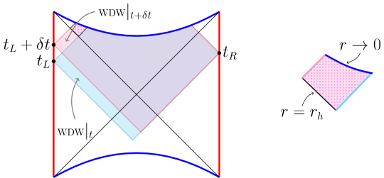
Figure 1: Two nearby Wheeler-de Witt patches at $t$ and $t+\delta t$ and the part that contributes to the late time behavior of complexity growth. This figure is drawn from Fig 2 of [12].

Therefore, we only need to consider the bulk action between two horizons, i.e.

$$\delta I_{\mathcal{M}} = I_{\mathcal{M}}\left[\text{WDW}|_{t+\delta t}\right]-I_{\mathcal{M}}\left[\text{WDW}|_{t}\right]$$ (2.5)

$$= \frac{1}{16\pi G}\int_{r\to 0}^{r_{h}}\int_{t}^{t+\delta t}\int_{S^{d}}\;\mathcal{L}_{F(R)}\;d\Omega_{d}\,dt\,dr\;\ \ \ \text{(at late time)}$$

$$= \frac{1}{16\pi G}\int_{r\to 0}^{r_{h}}\int_{t}^{t+\delta t}\int_{S^{d}}\;r^{d}\;F(R)\;d\Omega_{d}\,dt\,dr=\frac{\Omega_{d}F(R)}{16\pi G(d+1)}r_{h}^{d+1}\,\delta t\,.$$

On the other hand from the generalized Gibbons-Hawking term evaluated at the horizon and singularity one finds

$$\delta I_{\partial\mathcal{M}} = \frac{1}{8\pi G}\int_{t}^{t+\delta t}\int_{\Omega^{d}}dt\,d\Omega_{d}\;\left[-\sqrt{f}\;\partial_{r}\left(r^{d}\sqrt{f}\right)F^{\prime}(R)\right]\Big{|}_{r_{h}}$$ (2.6)

$$- \frac{1}{8\pi G}\int_{t}^{t+\delta t}\int_{\Omega_{d}}dt\,d\Omega_{d}\;\;\left[-\sqrt{f}\;\partial_{r}\left(r^{d}\sqrt{f}\right)F^{\prime}(R)\right]\Big{|}_{r\to 0}$$

$$= \frac{\Omega_{d}}{8\pi G}\left(d\,r_{h}^{d-1}+\frac{(d+1)r_{h}^{d+1}}{\ell^{2}}\right)F^{\prime}(R)\,\delta t$$

$$= -\frac{\Omega_{d}F(R)}{16\pi G(d+1)}((d+1)r_{h}^{2}+d\,\ell^{2})r_{h}^{d-1}\delta t.$$

Putting these expressions together one arrives at

$$\delta(I_{\cal M}+I_{\partial{\cal M}})=-\frac{\Omega_{d}F(R)d}{16\pi G(d+1)}(r_{h}^{2}+\ell^{2})r_{h}^{d-1}\delta t,$$ (2.7)

from which one can read the complexity growth for the eternal AdS-Schwarzschild black hole as follows

$${\dot{\cal C}}=\frac{dI}{dt}=2M_{F}$$ (2.8)

that, interestingly enough, saturates the complexity growth bound. Note that to find the above expression we have used the definition of the ADM mass given by (2.4).

3 CA for Critical Gravity

In this section we will study the complexity growth for yet another interesting theory containing higher derivative terms. The model we will be considering is “critical gravity” whose action is given by [17]

$$I=\frac{1}{16\pi G}\int_{\mathcal{M}}d^{d+2}x\sqrt{-g}\left[R-2\Lambda-\frac{1}{m^{2}}\left(R^{\mu\nu}R_{\mu\nu}-\frac{d+2}{4(d+1)}R^{2}\right)\right],$$ (3.1)

where $m$ is a dimensionful parameter. This model admits several solutions including AdS and AdS black holes with radius $\ell$. It is known that at the critical point where $m^{2}=\frac{d^{2}}{2\ell^{2}}$ the model degenerates yielding to a log-gravity [18].

It is useful to use an auxiliary field $f_{\mu\nu}$ to recast the action (3.1) into the following form

$$I=\frac{1}{16\pi G}\int_{\mathcal{M}}d^{d+2}x\sqrt{-g}\left[R-2\Lambda+f^{\mu\nu}G_{\mu\nu}+\frac{m^{2}}{4}\left(f^{\mu\nu}f_{\mu\nu}-f^{2}\right)\right],$$ (3.2)

where $G_{\mu\nu}$ is the Einstein tensor and the auxiliary field $f_{\mu\nu}$ is given by

$$f_{\mu\nu}=-\frac{2}{m^{2}}\left(R_{\mu\nu}-\frac{1}{2(d+1)}Rg_{\mu\nu}\right).$$ (3.3)

In this notation the generalized Gibbons-Hawking terms that make the variational principle for Dirichlet boundary condition well posed are[21]

$$I_{GGH}=\frac{1}{16\pi G}\int_{\partial\mathcal{M}}d^{d+1}x\sqrt{-\gamma}\left(-2K-\hat{f}^{ij}K_{ij}+\hat{f}K\right).$$ (3.4)

Here $K_{ij}$ is the extrinsic curvature of the boundary, $K$ is trace of the extrinsic curvature and the auxiliary field ${\hat{f}}^{ij}$ is defined as follows

$$\hat{f}^{ij}=f^{ij}+2h^{(i}N^{j)}+sN^{i}N^{j},$$ (3.5)

where the quantities appearing in this equation are defined via ADM decomposition of the metric

$$ds^{2}=N^{2}dr^{2}+\gamma_{ij}(dx^{i}+N^{i}dr)(dx^{j}+N^{j}dr),$$ (3.6)

and

$$f^{\mu\nu}=\left(\begin{array}[]{cc}s&h^{i}\\ h^{i}&f^{ij}\\ \end{array}\right)\,.$$ (3.9)

Note also that $\hat{f}=\gamma_{ij}\hat{f}^{ij}$. With this notation in what follows we will compute holographic complexity for this model using CA proposal.

3.1 Stationary solutions

In this subsection we would like to investigate the CA proposal of complexity for the critical gravity. As we have already mentioned in order to compute the complexity the main challenge is to find the contribution of the boundary terms. In what follows we will use the approach of [12] to calculate the late time growth of complexity.

To start, let us consider three dimensional case (known as NMG model[22])where one could have a rotating BTZ black hole whose metric may be given by

$$ds^{2}=\frac{dr^{2}}{f(r)}-f(r)dt^{2}+r^{2}\left(d\phi-\frac{8GJ}{2r^{2}}dt\right)^{2},\;\;\;\;\;\;\;\;f(r)=\frac{r^{2}}{\ell^{2}}-8GM+\frac{(8GJ)^{2}}{4r^{2}}.$$ (3.10)

The parameters $M$ and $J$ can be expressed in terms of the outer and inner horizon radii, $r_{+},r_{-}$ that are solutions of the equation $f(r)=0$. More explicitly, one has

$$f(r)=\frac{(r^{2}-r_{+}^{2})(r^{2}-r_{-}^{2})}{r^{2}\ell^{2}},\hskip 14.22636pt8GM=\frac{r_{+}^{2}+r_{-}^{2}}{\ell^{2}},\hskip 14.22636pt8GJ=\frac{2r_{+}r_{-}}{\ell}.$$ (3.11)

It is however important to note that $M$ and $J$ are the parameters of the solution and not the physical quantities. Indeed the ADM mass and angular momentum of the solution that depend on the explicit form of action are given by[21]

$$M_{\rm NMG}=M\left(1-\frac{1}{2\ell^{2}m^{2}}\right),\hskip 14.22636ptJ_{\rm NMG}=J\left(1-\frac{1}{2\ell^{2}m^{2}}\right).$$ (3.12)

To compute the complexity growth one needs to consider difference between on-shell action evaluated over two nearby WDW patches depicted in the Fig 2.

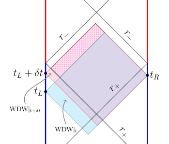
Figure 2: Two nearby Wheeler-de Witt patches for BTZ black hole at $t$ and $t+\delta t$ and the part that contributes to the late time behavior of complexity growth.This figure is drawn from Fig 4 of [12].

At the late time the only region which lies between two horizons contributes to this difference. Therefore one gets

$$\delta I_{\mathcal{M}} = I_{\mathcal{M}}\left[\text{WDW}|_{t+\delta t}\right]-I_{\mathcal{M}}\left[\text{WDW}|_{t}\right]$$ (3.13)

$$= \frac{1}{16\pi G}\int_{r_{-}}^{r_{+}}\int_{t}^{t+\delta t}\int_{0}^{2\pi}\;\mathcal{L}_{\rm NMG}\;d\phi\,dt\,dr\;\ \ \ \text{(at late time)}$$

$$= -\frac{2\pi\delta t}{16\pi G}\int_{r_{-}}^{r_{+}}\frac{4r}{\ell^{2}}\left(1-\frac{1}{2\ell^{2}m^{2}}\right)dr=-\frac{(r_{+}^{2}-r_{-}^{2})}{4G\ell^{2}}\left(1-\frac{1}{2\ell^{2}m^{2}}\right)\delta t.$$

The contribution of the generalized Gibbons-Hawking terms (3.4) are also given by

$$\delta I_{\partial\mathcal{M}} = \frac{1}{16\pi G}\int_{t}^{t+\delta t}\int_{0}^{2\pi}dt\,d\phi\;\left[\frac{-2}{\ell^{2}}(r_{+}^{2}+r_{-}^{2}-2r^{2})\left(1-\frac{1}{2\ell^{2}m^{2}}\right)\right]\Big{|}_{r_{+}}$$ (3.14)

$$-\frac{1}{16\pi G}\int_{t}^{t+\delta t}\int_{0}^{2\pi}dt\,d\phi\;\left[\frac{-2}{\ell^{2}}(r_{+}^{2}+r_{-}^{2}-2r^{2})\left(1-\frac{1}{2\ell^{2}m^{2}}\right)\right]\Big{|}_{r_{-}}$$

$$= \frac{(r_{+}^{2}-r_{-}^{2})}{2G\ell^{2}}\left(1-\frac{1}{2\ell^{2}m^{2}}\right){\delta t}.$$

Therefore, one arrives at

$$\frac{dI}{dt}\equiv\frac{dI_{\mathcal{M}}}{dt}+\frac{dI_{\partial\mathcal{M}}}{dt}=\frac{(r_{+}^{2}-r_{-}^{2})}{4G\ell^{2}}\left(1-\frac{1}{2\ell^{2}m^{2}}\right),$$ (3.15)

which is the total rate of growth of the action. By making use of equations (3.11) and (3.12) the above expression reads

$${\dot{\cal C}}=\frac{dI}{dt}=2\sqrt{M^{2}-\frac{J^{2}}{\ell^{2}}}\left(1-\frac{1}{2\ell^{2}m^{2}}\right)=2\sqrt{M_{\rm NMG}^{2}-\frac{J_{\rm NMG}^{2}}{\ell^{2}}},$$ (3.16)

thats is consistent with results of [12].

Encouraged by this result let us consider higher dimensional critical gravity. It is easy to see that the equations of motion obtained from the action (3.1) admits the AdS-Schwarzschild black hole whose metric is given by

$$ds^{2}=\frac{dr^{2}}{f(r)}-f(r)dt^{2}+r^{2}d\Omega^{2}_{d},\;\;\;\;\;\;\;\;\;\;f(r)=\frac{r^{2}}{\ell^{2}}+1-\frac{8\pi}{d\,\Omega_{d}}\frac{2GM}{r^{d-1}}.$$ (3.17)

where $M$ is a parameter of the solution (not the physical mass) and the radius $\ell$ satisfies the following equation

$$\frac{2\Lambda}{d(d+1)}\ell^{4}+\ell^{2}-\frac{d(d-2)}{4m^{2}}=0.$$ (3.18)

Once again we would like to calculate the on-shell action over difference of two WDW patches corresponding to two states at the late time. Doing so one finds

$$\delta I_{\mathcal{M}} = I_{\mathcal{M}}\left[\text{WDW}|_{t+\delta t}\right]-I_{\mathcal{M}}\left[\text{WDW}|_{t}\right]$$ (3.19)

$$= \frac{1}{16\pi G}\int_{r\to 0}^{r_{h}}\int_{t}^{t+\delta t}\int_{S^{d}}\;\mathcal{L}_{\rm CG}\;d\Omega_{d}\,dt\,dr\;\ \ \ \text{(at late time)}$$

$$= \frac{\Omega_{d}\,\delta t}{16\pi G}\int_{r\to 0}^{r_{h}}r^{d}\left(-2\frac{d+1}{\ell^{2}}\right)\left(1-\frac{d^{2}}{2\ell^{2}m^{2}}\right)dr=-\frac{\Omega_{d}r_{h}^{d+1}}{8\pi G\ell^{2}}\left(1-\frac{d^{2}}{2\ell^{2}m^{2}}\right)\delta t.$$

In addition, the contribution of the generalized Gibbons-Hawking terms are

$$\delta I_{\partial\mathcal{M}} = \frac{1}{16\pi G}\int_{t}^{t+\delta t}\int_{S^{d}}dt\,d\Omega_{d}\;\left[-2\sqrt{f}\;\partial_{r}\left(r^{d}\sqrt{f}\right)\left(1-\frac{d^{2}}{2\ell^{2}m^{2}}\right)\right]\Big{|}_{r_{h}}$$ (3.20)

$$-\frac{1}{16\pi G}\int_{t}^{t+\delta t}\int_{S^{d}}dt\,d\Omega_{d}\;\;\left[-2\sqrt{f}\;\partial_{r}\left(r^{d}\sqrt{f}\right)\left(1-\frac{d^{2}}{2\ell^{2}m^{2}}\right)\right]\Big{|}_{r\to 0}$$

$$= \frac{\Omega_{d}}{8\pi G}\left(d\,r_{h}^{d-1}+\frac{(d+1)r_{h}^{d+1}}{\ell^{2}}\right)\left(1-\frac{d^{2}}{2\ell^{2}m^{2}}\right)\delta t.$$

Here we have considered the contribution of the generalized Gibbons-Hawking terms at the horizon $r_{h}$ and the singularity $r\to 0$. Taking bulk and boundary contributions into account one arrives at

$${\dot{\cal C}}=\frac{dI}{dt}\equiv\frac{dI_{\mathcal{M}}}{dt}+\frac{dI_{\partial\mathcal{M}}}{dt}=2M\left(1-\frac{d^{2}}{2\ell^{2}m^{2}}\right)=2M_{\rm HD}\,.$$ (3.21)

Here to write the final expression we have used the relation between the parameter $M$ and the physical mass $M_{\rm HD}$ of the critical gravity[17]. Interestingly enough this is also consistent with the general expectation of [12].

Note that at the critical point, $m^{2}=\frac{d^{2}}{2\ell^{2}}$ where the model develops a log gravity, the rate of growth vanishes. Actually at this point one has to redo the computation from the first step with a logarithmic solution that is a time-dependent solution.

3.2 Localized Shock wave solutions

In this subsection in order to arrive at a deeper understanding of the effects of higher derivatives terms in the growth of complexity we will study complexity growth in a black hole perturbed by a shock wave. To proceed, following [12] we will consider the evaluation of thermofield double state perturbed by a single precursor as follows

$$e^{-iH_{L}t_{L}}e^{-iH_{R}t_{R}}W_{x}(t_{w})\mid\text{TFD}\hskip 1.42262pt\rangle.$$ (3.22)

$H_{L}$ and $H_{R}$ are Hamiltonians of the left and right boundary, respectively and

$$W_{x}(t_{w})=e^{-iHt_{w}}W_{x}e^{iHt_{w}},$$ (3.23)

with $W_{x}$ being a simple operator acting on the left boundary. For $t_{w}=0$, the precursor operator is a local operator in the thermal scale, though it becomes nonlocal by increasing the time $|t_{w}|>0$. In our notations the shock wave emerges at the left boundary at $t_{w}<0$ and we are interested in the region where $t_{L},t_{R}>0$. The geometry dual to the state (3.22) can be described by a shock wave solution whose metric in the Kruskal coordinates may be given as follows[24]

$$ds^{2}=-2A(uv)dudv+B(uv)d\Omega^{2}_{d}+2A(uv)h(x)\delta(u)du^{2},$$ (3.24)

(3.25)

$$A(uv)=-\frac{2}{uv}\;\frac{f(r)}{f^{2}(r_{H})},\;\;\;\;\;\;\;\;\;\;B(uv)=r^{2},$$ (3.26)

where $f(r)$ is given in (3.17) and the Kruskal coordinates in terms of the Schwarzschild coordinates are given by

$$u=\exp[\frac{2\pi}{\beta}(r_{\ast}(r)-t)],\hskip 14.22636ptv=-\exp[\frac{2\pi}{\beta}(r_{\ast}(r)+t)],\hskip 14.22636pt\beta=\frac{4\pi\ell^{2}}{(d+1)r_{h}+(d-1)\frac{\ell^{2}}{r_{h}}},$$ (3.27)

with $dr_{\ast}=dr/f(r)$. The shock wave strength $h(x)$ may be found from the equations of motion when the back reaction of the local operator $W_{x}$ is also taken into account. For Einstein gravity the shock wave was studied in [24]. The Kruskal diagram of the geometry (3.24) is shown in Fig.3 (see Fig 8 of [12]).

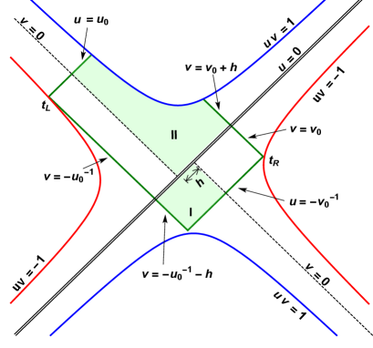
Figure 3: Kruskal diagram of one-shock geometries. The double black line along $u=0$ is the shock wave. The green lines show the boundary of WDW patch. The green shaded region is the intersection of WDW and the black hole interior. In this figure a small shift $h(x)$ with $h(x)<v_{0}$ is drown. For a large shift $h(x)$ with $h(x)>v_{0}$ the boundary of WDW intersect the past singularity $uv=1$. This figure is drown from Fig 8 of [12].

As it is clear from the figure, one recognizes two distinctive cases depending on the size of the shift $h(x)$. Actually for a small shift where $u_{0}^{-1}+h(x)<v_{0}$ the boundary of WDW does not intersect the past singularity leading to a diamond shape ( region $I$ in the Fig 3). On the other hand for large shift where $u_{0}^{-1}+h(x)\geq v_{0}$ the past singularity is also intersected by the WDW patch leading to a five-sided region similar to region $II$ drown in Fig 3. In the latter case both regions above and below $u=0$ axis are five-sided regions bounded by two edges of WDW patch, two horizons and a singularity. As it was argued in [12] due to the fact that we are interested in large $t_{R}>0$, where $v_{0}^{-1}$ is exponentially small, the contribution to the action comes from five-sided regions and that of diamond vanishes. It is worth mentioning that in the Kruskal coordinates one has

$$u_{0}=\exp[\frac{2\pi}{\beta}t_{L}],\hskip 28.45274ptv_{0}=\exp[\frac{2\pi}{\beta}t_{R}].$$ (3.28)

Let us now consider the growth of complexity for a shock wave in the critical gravity. To proceed we need to find a shock wave solution in a black hole solution of the critical gravity. We note however that following [12] in order to avoid difficulties of having a spatially compact boundary, one may consider the planar-AdS black hole geometry.

In critical gravity the planer shock wave has been studied in [25] where it was shown that due to higher derivative terms there are two butterfly velocities and

$$h(x)\sim e^{\frac{2\pi}{\beta}(\mid t_{w}\mid-t_{\ast}-\frac{\mid x\mid}{v_{B}^{(1)}})}-\frac{v_{B}^{(2)}}{v_{B}^{(1)}}e^{\frac{2\pi}{\beta}(\mid t_{w}\mid-t_{\ast}-\frac{\mid x\mid}{v_{B}^{(2)}})},$$ (3.29)

where $\lambda_{L}=\frac{2\pi}{\beta}$ is the Lyapunov exponent, $t_{\ast}$ is the scrambling time, and the butterfly velocities are given by

$$v_{B}^{(1)}=\sqrt{\frac{d+1}{2d}},\hskip 28.45274ptv_{B}^{(2)}=\sqrt{\frac{d+1}{2d}}\frac{1}{\sqrt{1+\frac{2\ell^{2}}{d(d+1)}M^{2}}},$$ (3.30)

with $M^{2}=\frac{2m^{2}\ell^{2}-d^{2}}{2\ell^{2}}$ being the mass of spin-2 massive mode. From these expression it is clear that $v_{B}^{(1)}>v_{B}^{(2)}$.

In what follows we would like to compute the on-shell action of the critical gravity for a shock wave solution whose shift $h(x)$ is given by (3.29). To do so we will consider both small and large shift cases.

As we have already mentioned for small shift the WDW patch consists of two parts: one five-sided and a diamond. Since ince $v_{0}^{-1}=\exp[-\frac{2\pi}{\beta}t_{R}]\ll 1$, the diamond region is exponentially small and has a vanishing contribution to the action and therefore one only needs to compute the contribution of the five-sided region. The corresponding contribution contains both the bulk and boundary parts. Taking into account that we are in the small shift region where $h(x)<v_{0}$ one finds

$$I_{\mathcal{M}}=-\frac{L^{d}r_{h}^{d+1}}{8\pi G\ell^{2}}\left(1-\frac{d^{2}}{2\ell^{2}m^{2}}\right)\frac{\beta}{2\pi}\log{u_{0}v_{0}},$$ (3.31)

and

$$I_{\partial\mathcal{M}}=-\left[\frac{L^{d}}{8\pi G}\left(d\,r^{d-1}+\frac{(d+1)r^{d+1}}{\ell^{2}}\right)\left(1-\frac{d^{2}}{2\ell^{2}m^{2}}\right)\right]^{r_{h}}_{0}\frac{\beta}{2\pi}\log{u_{0}v_{0}}.$$ (3.32)

Note that the generalized Gibbons-Hawking terms are computed at the singularity and at the horizon. Here $L^{d}$ is spatial volume of the internal space. Putting everything together one arrives at

$$I=2M_{\text{HD}}(t_{L}+t_{R}).$$ (3.33)

To get this expression we have used the equation (3.28) and the definition of physical mass in critical gravity. It is exactly the same form we have for the Einstein gravity except with inserting the proper mass of the model. This expression might be understood from the fact that at small shift the explicit form of $h(x)$ does not play an essential role. In other words it means that for large $t_{R}$, we have evolved the state to a region where the back-reaction of perturbation (precursor operator) is negligible and the complexity is simply given by time evolution of TFD state.

Let us now consider the big shift where $h(x)>v_{0}$. In this case we have to deal with a WDW patch consisting of two parts in the shape of the five-sided region and therefore both parts contribute to the on-shell action. The contribution of the upper five-sided region (taking onto account bulk and boundary terms) is

$$I_{\text{upper}}=\frac{L^{d-1}}{8\pi G}\left(dr_{h}^{d-1}+\frac{dr_{h}^{d+1}}{\ell^{2}}\right)\left(1-\frac{d^{2}}{2\ell^{2}m^{2}}\right)\frac{\beta}{2\pi}\int dx\hskip 2.84526pt\log[u_{0}h(x)],$$ (3.34)

while that of lower one is

$$I_{\text{lower}}=\frac{L^{d-1}}{8\pi G}\left(dr_{h}^{d-1}+\frac{dr_{h}^{d+1}}{\ell^{2}}\right)\left(1-\frac{d^{2}}{2\ell^{2}m^{2}}\right)\frac{\beta}{2\pi}\int dx\hskip 2.84526pt\log[v_{0}^{-1}h(x)].$$ (3.35)

To find the above expression we have used that fact at $h(x)>v_{0}$ and $u_{0}^{-1}\ll 1$. Moreover the overall factor $L^{d-1}$ in both expressions comes from the fact that the corresponding shock wave (3.29) is localized in one transverse direction. From equations (3.34) and(3.35) one arrives at

$$I=\frac{L^{d-1}}{8\pi G}\left(dr_{h}^{d-1}+\frac{dr_{h}^{d+1}}{\ell^{2}}\right)\left(1-\frac{d^{2}}{2\ell^{2}m^{2}}\right)\frac{\beta}{2\pi}\int dx\hskip 2.84526pt\log[u_{0}v_{0}^{-1}h^{2}(x)].$$ (3.36)

On the other hand by making use of equations (3.29) and (3.28), the integrand part of the above equation may be simplified as follows

$$\frac{\beta}{2\pi}\log[u_{0}v_{0}^{-1}h^{2}(x)]=(t_{L}+t_{R})+2\left(|t_{w}|-t_{\ast}-t_{R}-\frac{|x|}{v_{B}^{(1)}}\right)+2\hskip 2.84526pt\frac{\beta}{2\pi}\log\left[1-\frac{v_{B}^{(2)}}{v_{B}^{(1)}}e^{-\frac{2\pi}{\beta}(\frac{1}{v_{B}^{(2)}}-\frac{1}{v_{B}^{(1)}})|x|}\right].$$ (3.37)

It is now easy to perform the integration over $x$ to get the following expression for the on-shell action

$$I = 2M_{\text{HD}}\left(t_{L}+t_{R}\right)+4\tilde{M}L^{d-1}\frac{v_{B}^{(1)}}{2}\bigg{(}\mid t_{w}\mid-t_{\ast}-t_{R}\bigg{)}^{2}$$ (3.39)

$$-4\tilde{M}L^{d-1}\frac{\beta^{2}}{4\pi^{2}}\frac{v_{B}^{(1)}v_{B}^{(2)}}{(v_{B}^{(1)}-v_{B}^{(2)})}\left[{\rm Li}_{2}\left(\frac{v_{B}^{(2)}}{v_{B}^{(1)}}\right)-{\rm Li}_{2}\left(\frac{v_{B}^{(2)}}{v_{B}^{(1)}}e^{\frac{-2\pi(v_{B}^{(1)}-v_{B}^{(2)})(\mid t_{w}\mid-t_{\ast}-t_{R})}{v_{B}^{(2)}\beta}}\right)\right],$$

where $\tilde{M}$ is the spatial energy density of the corresponding black hole and ${\rm Li}_{2}(x)$ is the dilogarithm function. It is worth noting that to find the above expression we have used the fact that we are in the big shift approximation where $h(x)>v_{0}$ we have

$$e^{\frac{2\pi}{\beta}\big{(}\mid t_{w}\mid-t_{\ast}-t_{R}\big{)}}\left(1-\frac{v_{B}^{(2)}}{v_{B}^{(1)}}e^{-\frac{2\pi}{\beta}\left(\frac{1}{v_{B}^{(2)}}-\frac{1}{v_{B}^{(1)}}\right)\mid x\mid}\right)>1,$$ (3.40)

and the integration over direction $x$ has been performed in the range of $0\leq x\leq v_{B}^{(1)}(|t_{w}|-t_{\ast}-t_{R})$. Actually one observes that the first two terms in equation (3.39) are the same as those in Einstein gravity [12], though the last term is the effect of higher derivative terms that slows down the rate of complexity growth.

4 Discussions

In this paper using “complexity=action” proposal, we have studied complexity of black hole solutions in some certain gravitational theories. In this proposal the complexity of a holographic state is given by the on-shell action evaluated on the Wheeler-De Witt patch. The main challenge to evaluate the on-shell action is to find the contribution of boundary terms defined on different time like or null boundaries or on intersection of these boundaries.

Although for the Einstein gravity these null boundary terms have been recently obtained in [15], for a general higher derivative action such boundary terms are not known. Indeed it is worth mentioning that even the standard Gibbons-Hawking terms for general action have not fully understood yet. In order to circumvent this issue, following [12] we will compute the rate of complexity growth in which the generalized Gibbons-Hawking boundary terms are enough. Of course we have considered certain gravitational theories with higher order terms whose generalized Gibbons-Hawking terms are known. These include $F(R)$-gravity and critical gravity in diverse dimensions. Encouraged by the results of [16] we would expect that the final results are independent of the missing null boundary terms of our models.

We have shown that for the neutral black hole solution the complexity growth saturates the proposed bound when the results are written in terms of physical quantities of the model under consideration

$${\dot{\cal C}}=2M,$$ (4.1)

where $M$ is the physical mass (ADM mass ) of the corresponding black hole (see also [26] for massive gravity). It was important to note that in higher derivative gravities the parameter that explicitly appears in the solution is not necessarily the physical mass of the solution.

We have also studied the effect of a single shock wave in the growth of complexity in the critical gravity. Due to the presence of higher derivative terms in the action the shock wave in the critical gravity propagates with two different butterfly velocities. We have seen that the complexity growth are affected by both velocities. Although the effect of massless mode is similar to that of Einstein gravity the effect of massive mode slows down the rate of complexity growth. Since we do not have a good understanding of complexity in the field theory dual, it might be hard to confirm this behavior from field theory point of view. Therefore our results should be treated as a prediction for the holographic complexity.

We could have also studied complexity growth for a shock wave in $F(R)$ gravity. We note, however, that since the model has only massless gravity mode, the situation would qualitatively be similar to that of Einstein gravity. This might be understood from the fact that $F(R)$ gravity may be map to an Einstein gravity coupled to a scaler field. In this case one gets only one butterfly velocity which comes from the gravitational part that could affect the growth.

As a final remark we would like to recall that there is another proposal for complexity known as “complexity=volume” or in short CV proposal [10, 28, 29, 30]. It is also expected [5] that in the presence of higher derivative terms one needs to extend the notion of volume to a new quantity. The situation is similar to thermal and entanglement entropies where the area must be replaced by certain functional to be evaluated on the horizon and RT curve, respectively (see e.g. [31]). As for complexity we would also like to have a new functional to be evaluated on a co-dimension one hypersurface. Although it is not clear to us whether the CV proposal fulfills all requirements to be identified with complexity, since in the cases we have been considering in the previous sections we would expect that CV and CA proposal would qualitatively match, in what follows we shall suggest two possibilities that are consistent with our results presented in the previous sections.

Motivated by Wald formula for entropy one may consider an expression which has a Wald-like form. To be precise consider a co-dimension one time slice whose normal vector is given by $n_{\mu}^{1}$. Then let us foliate the co-dimension one hypersurface alone the radial coordinate parametrized by the normal vector $n_{\mu}^{2}$. Having two normal vector one may construct a binormal anti-symmetric 2-tensor by which we can compute Wald integrand as follows

$$\frac{\partial\mathcal{L}}{\partial R_{\mu\nu\alpha\beta}}\epsilon_{\mu\nu}\epsilon_{\alpha\beta}.$$ (4.2)

Now the natural proposal for CV complexity is[5]

$$C_{V}=-\frac{1}{\ell}\int_{\cal B}\frac{\partial\mathcal{L}}{\partial R_{\mu\nu\alpha\beta}}\epsilon_{\mu\nu}\epsilon_{\alpha\beta},$$ (4.3)

where $\ell$ is a length scale in the bulk gravity and ${\cal B}$ is a co-dimension one maximal time slice. Using the explicit expressions of Ricci and scalar curvature for Black hole solutions in the critical gravity (3.17) one gets

$$\frac{\partial\mathcal{L}_{\text{HD}}}{\partial R_{\mu\nu\alpha\beta}}\epsilon_{\mu\nu}\epsilon_{\alpha\beta}=-2\left(1-\frac{d^{2}}{2\ell^{2}m^{2}}\right).$$ (4.4)

Plugging this expression in the equation (4.3) one finds the CV complexity for the critical gravity which is consistent with our results found in the previous section.

On the other hand in the context of the entanglement equilibrium the authors of [32] has found an expression for volume that kept fixed while varying the entanglement entropy. Based on this result the authors have proposed an expression for CV complexity which is given as follows. Let us denote the normal vector to the time slice hypersurface by $n^{\mu}$ and define the following functional for given Lagrangian

$$\frac{\partial\mathcal{L}}{\partial R_{\mu\nu\alpha\beta}}\left(a\hskip 2.84526ptn_{\mu}n_{\beta}h_{\nu\alpha}+b\hskip 2.84526pth_{\mu\beta}h_{\nu\alpha}\right)+c,$$ (4.5)

where $a,\,b$ and $c$ are three arbitrary constants. Then the generalized CV complexity may be defined as follows

$$C_{V}=-\frac{1}{\ell}\int_{\cal B}\left[\frac{\partial\mathcal{L}}{\partial R_{\mu\nu\alpha\beta}}\left(a\hskip 2.84526ptn_{\mu}n_{\beta}h_{\nu\alpha}+b\hskip 2.84526pth_{\mu\beta}h_{\nu\alpha}\right)+c\right],$$ (4.6)

where as before $\ell$ is a length scale in the bulk gravity and ${\cal B}$ is a co-dimension one maximal time slice. Since the complexity in terms of volume may be defined up to an overall factor of order one, we may set $a=1$. It is an easy excesses to evaluate the above functional for the black hole solution (3.17) in critical gravity. Doing so one arrives at

$$\frac{\partial\mathcal{L}_{\text{HD}}}{\partial R_{\mu\nu\alpha\beta}}\left(\hskip 2.84526ptn_{\mu}n_{\beta}h_{\nu\alpha}+b\hskip 2.84526pth_{\mu\beta}h_{\nu\alpha}\right)+c=\frac{d+1}{2}(1-d\,b)\left(1-\frac{d^{2}}{2\ell^{2}m^{2}}\right)+c.$$ (4.7)

It is then clear that to get a consistent result one should set $c=0$ and $b=\frac{d+5}{d(d+1)}$. Since in this definition the generalized volume is ambiguous up to an overall factor of order one, different $a$ and $b$ may also be chosen, though it seems that the constant $c$ should always be set to zero.

Definitely it would be interesting to further explore properties of the above proposals for the generalized volume and to their connection with holographic complexity.

References

- [1] G. W. Gibbons and S. W. Hawking, “Action integrals and partition functions in quantum gravity,” Phys. Rev. D 15, 2752 (1977)
- [2] J. M. Maldacena, “The Large N limit of superconformal field theories and supergravity,” Int. J. Theor. Phys. 38, 1113 (1999) [Adv. Theor. Math. Phys. 2, 231 (1998)] doi:10.1023/A:1026654312961 [hep-th/9711200].
- [3] M. Henningson and K. Skenderis, “The Holographic Weyl anomaly,” JHEP 9807, 023 (1998) doi:10.1088/1126-6708/1998/07/023 [hep-th/9806087].
- [4] C. R. Graham and E. Witten, “Conformal anomaly of submanifold observables in AdS / CFT correspondence,” Nucl. Phys. B 546, 52 (1999) doi:10.1016/S0550-3213(99)00055-3 [hep-th/9901021].
- [5] M. Alishahiha, “Holographic Complexity,” Phys. Rev. D 92, no. 12, 126009 (2015) doi:10.1103/PhysRevD.92.126009 [arXiv:1509.06614 [hep-th]]. Talk given at “Recent Trends in String Theory and Related Topics 23-30 May, 2016” http://physics.ipm.ac.ir/conferences/stringtheory/note/M.Alishahaiha.pdf
- [6] O. Ben-Ami and D. Carmi, “On Volumes of Subregions in Holography and Complexity,” JHEP 1611, 129 (2016) doi:10.1007/JHEP11(2016)129 [arXiv:1609.02514 [hep-th]].
- [7] S. Ryu and T. Takayanagi, “Holographic derivation of entanglement entropy from AdS/CFT,” Phys. Rev. Lett. 96, 181602 (2006) [hep-th/0603001].
- [8] M. Alishahiha, unpublished.
- [9] L. Susskind, “Computational Complexity and Black Hole Horizons,” Fortsch. Phys. 64, 24 (2016) doi:10.1002/prop.201500092 [arXiv:1403.5695 [hep-th], arXiv:1402.5674 [hep-th]].
- [10] D. Stanford and L. Susskind, “Complexity and Shock Wave Geometries,” Phys. Rev. D 90, no. 12, 126007 (2014) doi:10.1103/PhysRevD.90.126007 [arXiv:1406.2678 [hep-th]].
- [11] A. R. Brown, D. A. Roberts, L. Susskind, B. Swingle and Y. Zhao, “Holographic Complexity Equals Bulk Action?,” Phys. Rev. Lett. 116, no. 19, 191301 (2016) doi:10.1103/PhysRevLett.116.191301 [arXiv:1509.07876 [hep-th]].
- [12] A. R. Brown, D. A. Roberts, L. Susskind, B. Swingle and Y. Zhao, “Complexity, action, and black holes,” Phys. Rev. D 93, no. 8, 086006 (2016) doi:10.1103/PhysRevD.93.086006 [arXiv:1512.04993 [hep-th]].
- [13] S. Lloyd, “Ultimate physical limits to computation,” Nature 406 (2000) 1047, [arXiv:quant-ph/9908043]
- [14] K. Parattu, S. Chakraborty, B. R. Majhi and T. Padmanabhan, “A Boundary Term for the Gravitational Action with Null Boundaries,” Gen. Rel. Grav. 48, no. 7, 94 (2016) doi:10.1007/s10714-016-2093-7 [arXiv:1501.01053 [gr-qc]].
- [15] L. Lehner, R. C. Myers, E. Poisson and R. D. Sorkin, “Gravitational action with null boundaries,” Phys. Rev. D 94 (2016) no.8, 084046 doi:10.1103/PhysRevD.94.084046 [arXiv:1609.00207 [hep-th]].
- [16] S. Chapman, H. Marrochio and R. C. Myers, “Complexity of Formation in Holography,” arXiv:1610.08063 [hep-th].
- [17] H. Lu and C. N. Pope, “Critical Gravity in Four Dimensions,” Phys. Rev. Lett. 106, 181302 (2011). doi:10.1103/PhysRevLett.106.181302
- [18] M. Alishahiha and R. Fareghbal, “D-Dimensional Log Gravity,” Phys. Rev. D 83, 084052 (2011) doi:10.1103/PhysRevD.83.084052 [arXiv:1101.5891 [hep-th]].
- [19] R. G. Cai, S. M. Ruan, S. J. Wang, R. Q. Yang and R. H. Peng, “Action growth for AdS black holes,” JHEP 1609, 161 (2016) doi:10.1007/JHEP09(2016)161 [arXiv:1606.08307 [gr-qc]].
- [20] E. Dyer and K. Hinterbichler, “Boundary Terms, Variational Principles and Higher Derivative Modified Gravity,” Phys. Rev. D 79, 024028 (2009) doi:10.1103/PhysRevD.79.024028 [arXiv:0809.4033 [gr-qc]].
- [21] O. Hohm and E. Tonni, “A boundary stress tensor for higher-derivative gravity in AdS and Lifshitz backgrounds,” JHEP 1004, 093 (2010). doi:10.1007/JHEP04(2010)093 [arXiv:1001.3598 [hep-th]].
- [22] E. A. Bergshoeff, O. Hohm and P. K. Townsend, “Massive Gravity in Three Dimensions,” Phys. Rev. Lett. 102, 201301 (2009) doi:10.1103/PhysRevLett.102.201301 [arXiv:0901.1766 [hep-th]].
- [23] G. Anastasiou and R. Olea, “From conformal to Einstein Gravity,” Phys. Rev. D 94, no. 8, 086008 (2016) doi:10.1103/PhysRevD.94.086008 [arXiv:1608.07826 [hep-th]].
- [24] D. A. Roberts, D. Stanford and L. Susskind, “Localized shocks,” JHEP 1503, 051 (2015). doi:10.1007/JHEP03(2015)051 [arXiv:1409.8180 [hep-th]].
- [25] M. Alishahiha, A. Davody, A. Naseh and S. F. Taghavi, “On Butterfly effect in Higher Derivative Gravities,” JHEP 1611, 032 (2016). doi:10.1007/JHEP11(2016)032 [arXiv:1610.02890 [hep-th]].
- [26] W. J. Pan and Y. C. Huang, “Holographic complexity and action growth in massive gravities,” arXiv:1612.03627 [hep-th].
- [27] R. Q. Yang, “Strong energy condition and the fastest computers,” arXiv:1610.05090 [gr-qc].
- [28] M. Miyaji, T. Numasawa, N. Shiba, T. Takayanagi and K. Watanabe, “Distance between Quantum States and Gauge-Gravity Duality,” Phys. Rev. Lett. 115, no. 26, 261602 (2015) doi:10.1103/PhysRevLett.115.261602 [arXiv:1507.07555 [hep-th]].
- [29] J. Couch, W. Fischler and P. H. Nguyen, “Noether charge, black hole volume and complexity,” arXiv:1610.02038 [hep-th].
- [30] D. Carmi, R. C. Myers and P. Rath, “Comments on Holographic Complexity,” arXiv:1612.00433 [hep-th].
- [31] X. Dong, “Holographic Entanglement Entropy for General Higher Derivative Gravity,” JHEP 1401, 044 (2014) doi:10.1007/JHEP01(2014)044 [arXiv:1310.5713 [hep-th]].
- [32] P. Bueno, V. S. Min, A. J. Speranza and M. R. Visser, “Entanglement equilibrium for higher order gravity,” arXiv:1612.04374 [hep-th].