Reversible temperature exchange upon thermal contact

Abstract

According to a well-known principle of thermodynamics, the transfer of heat between two bodies is reversible when their temperatures are infinitesimally close. As we demonstrate, a little-known alternative exists: two bodies with temperatures different by an arbitrary amount can completely exchange their temperatures in a reversible way if split into infinitesimal parts that are brought into thermal contact sequentially.

I Introduction

This story dates back almost 30 years, when one of us, a high school teacher, found a curious note in an obscure Soviet book about a fascinating phenomenon.Mak He called the subject to the attention of his students, the other author being among them. As intriguing as the problem appeared, its complete solution eluded us for many years. And while we clearly cannot take credit of inventors of the main principle here—after all this principle has been used for decades in commercial heat exchangersexchanger —the present analysis of the problem, to our best understanding, is novel and in any case not commonly known to physics instructors.

It is hard to come up with a more basic thermodynamic question, or one that even those who have never studied physics might feel confident to answer. Consider equal amounts of icy cold ($0\,\degree\text{C}$) and steaming hot ($100\,\degree\text{C}$) water. One needs to cool the hot water as much as possible by bringing it in thermal contact with the cold water, but without actually mixing them. Heat losses to the environment are neglected.

Simply bringing the two waters into direct thermal contact would obviously result in the final temperature of $50\,\degree\text{C}$ for both, as long as the specific heat of water is assumed to be independent of temperature.capacity If, however, one first splits the cold water into two equal amounts and then brings them in contact with the entire amount of hot water one after another, the result is different. Indeed, after the first contact the hot water will cool down to

$$100\,\degree\text{C}\times\frac{2}{3}=66.67\,\degree\text{C}.$$ (1)

After the second contact, the temperature of the hot water will be

$$66.67\,\degree\text{C}\times\frac{2}{3}=44.44\,\degree\text{C},$$ (2)

which is well below the middle value of $50\,\degree\text{C}$. Correspondingly, the temperatures of the two parts of the (initially) cold water will be $66.67\,\degree\text{C}$ and $44.44\,\degree\text{C}$. Upon the subsequent mixing, they reach the final equilibrium temperature of $55.56\,\degree\text{C}$, which together with the final temperature of the formerly hot water, $44.44\,\degree\text{C}$, adds up to $100\,\degree\text{C}$.

One does not have to stop at splitting the cold water into merely two halves. Suppose that it is separated into $N$ equal parts and then, as before, each part is brought into contact with the whole body of the hot water. After the first contact the hot water will cool down to

$$\frac{t_{0}}{1+1/N},\hskip 14.22636ptt_{0}=100\,\degree\text{C}.$$ (3)

After the second contact its temperature will go down a bit more to

$$\frac{t_{0}}{\left(1+{1}/{N}\right)^{2}}.$$ (4)

After all $N$ cold parts have been used, the final temperature of the hot water will be

$$\frac{t_{0}}{\left(1+{1}/{N}\right)^{N}}.$$ (5)

In the limit of infinitely fine splitting, $N\to\infty$, the ultimate temperature will be

$$t_{0}/e=36.79\,\degree\text{C}.$$ (6)

Finally, all parts of the “cold” water are mixed together and, according to the conservation of energy, their final temperature must be $t_{0}(1-1/e)=63.21\,\degree\text{C}$, considerably warmer than the “hot” water. While the temperature of the latter is the same as the temperature of a human body, the “cold” water is too hot for a human to stand. But can one do even better?

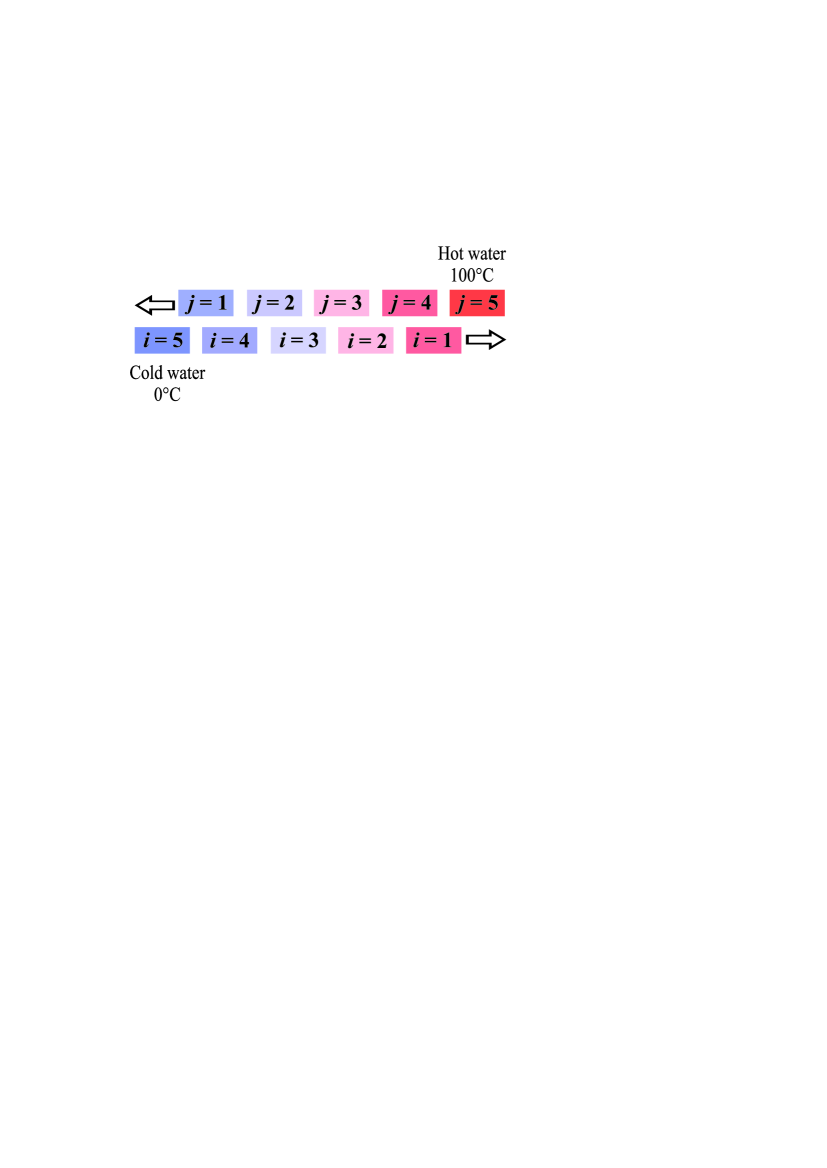
Figure 1: Schematic illustration of the heat exchange process: cold and hot waters are split into $N$ equal parts and brought into contact sequentially with one another, like oncoming trains passing. At each stop the water parts are allowed full thermal equilibration.

One should not stop at splitting only the cold water. Suppose that both the cold water and the hot water are split into two equal parts and the first cold part is brought into thermal contact with both hot parts in sequence; see Fig. 1 for the basic principle. The first cold part is then set aside and the remaining half of the cold water is brought in contact with the two parts of hot water, now somewhat cooled down by the passage of the first half of the cold water. To describe the entire process, it is convenient to construct the matrix shown in Fig. 2. The element $t_{ij}$ represents the equilibrium temperature established after the $i$th part of the cold water is brought in thermal contact with the $j$th part of the hot water. For example, after the first cold part makes contact with the first hot part, their common temperature is $t_{11}=(0\,\degree\text{C}+100\,\degree\text{C})/2=50\,\degree\text{C}$. After the same cold part is brought into contact with the second hot part, their eventual equilibrium temperature is $t_{12}=(50\,\degree\text{C}+100\,\degree\text{C})/2=75\,\degree\text{C}$.

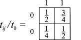
Figure 2: The matrix elements $t_{ij}$ show the temperature of the $i$th part of the cold water after it makes thermal contact with the $j$th part of the hot water, when both are split into $N=2$ parts.

When the second cold part moves through the sequence of hot parts, the initial temperatures of those hot parts are equal to the equilibrium temperatures achieved after their previous heat exchanges, given by the elements of the previous row. One can, therefore, determine the general rule for the construction of the temperature matrix:

$$t_{ij}=\frac{1}{2}\Bigl{(}t_{i-1,j}+t_{i,j-1}\Bigr{)}.$$ (7)

We can extend this recurrence relation to include even the first row and the first column by introducing the “zero” row and “zero” column,

$$t_{0j}=t_{0},\hskip 14.22636ptt_{i0}=0\,\degree\text{C},$$ (8)

which represent the initial temperatures of the hot and cold parts, respectively.

The final temperature of the (initially) cold water, after all $N^{2}$ thermal exchanges are completed, is given by the average of the entries in the last column; and the final temperature of the (initially) hot water is given by the average of the entries in the last row:

$$t_{\rm cold}(N)=\frac{1}{N}\sum_{i=1}^{N}t_{iN},\hskip 14.22636ptt_{\rm hot}(N)=\frac{1}{N}\sum_{j=1}^{N}t_{Nj}.$$ (9)

Taking the average of the last row in Fig. 2, one finds the final temperature of the hot water to be, $t_{\rm hot}(2)=(75\,\degree\text{C}+50\,\degree\text{C})/2=37.5\,\degree\text{C}$. Thus, by splitting both waters into just two parts we have done almost as well as by splitting only one into infinitely many parts.

We can do significantly better by making $N=3$ splits. In that case the matrix of temperature elements is shown in Fig. 3 and the final temperature is $t_{\rm hot}(3)=t_{0}(1/8+5/16+1/2)/3=31.25\,\degree\text{C}$.

Figure 3: The elements of the temperature matrix for $N=3$ parts.

The natural question is this: what is the lowest temperature that the hot water can be cooled down to if the number of splittings is increased indefinitely, $N\to\infty$? In Sec. II we demonstrate that in this limit a complete temperature inversion occurs, and that with a very good accuracy the ultimate temperature obeys the simple formula

$$t_{\rm hot}(N)\approx\frac{t_{0}}{\sqrt{\pi N}}.$$ (10)

This result raises the next question: how is it possible that the outcome of clearly irreversible heat exchanges between bodies with different temperatures is nonetheless a reversible process? Indeed, the simplest definition of a reversible process in thermodynamics is that the process changes direction upon an infinitesimal change of the conditions.LL For example, the heat exchange between two bodies with temperatures that differ by an infinitesimal amount is reversible. More rigorously, a process is reversible if the net change of the entropy of all bodies involved is zero,LL ; Sam ; Rec ; Bat $\Delta S=0$. Correspondingly, when the bodies brought in thermal contact have a non-infinitesimal temperature difference, the net entropy change is nonzero and thus the process is irreversible.

The thermal exchange with an infinite number of parts ($N\to\infty$) described in this paper represents a distinct type of reversible process. Note that a reversible process facilitated by an infinite number of thermal baths is well studied in the existing literature.Gal ; Gup ; McL ; Hei ; Tho ; Mir ; Cra ; Ana ; Ana1 We emphasize, however, that the scenario described here is quite different: the reversibility does not rely on the presence of any auxiliary bodies as there are no thermal baths involved.

In the following section we calculate the final temperatures of the hot and cold waters for arbitrary $N$. In Sec. III we treat the continuum limit, $N\to\infty$, directly. We then address the question of the net entropy change in Sec. IV.

II The case of arbitrary $N$

The recurrence relations (7) together with the “boundary conditions” (8) determine the whole matrix $t_{ij}$ for an arbitrary number $N$ of rows and columns. Some general properties of this matrix become clear from the simpler cases of $N=2$ and 3 considered above. We observe that the diagonal elements all equal $t_{0}/2$ and that any element and its transpose add up to $t_{0}$:

$$t_{ij}+t_{ji}=t_{0},\hskip 14.22636ptt_{ii}=t_{0}/2.$$ (11)

The same properties (11) remain valid for any size of the matrix, as illustrated by Fig. 4 for $N=6$.

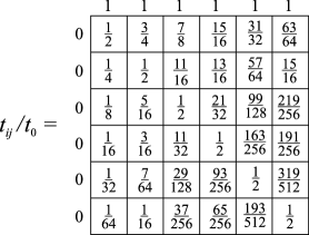
Figure 4: The elements of the temperature matrix $t_{ij}$ for $N=6$ parts.

Let us find the value of an element $t_{ij}$ for arbitrary $i$ and $j$. According to the recurrence relation (7), any element is determined by its neighbors that are immediately above and immediately to the left. An element $t_{ij}$ therefore ultimately “acquires” its value from those and only those initial elements $t_{0k}$ that have $k\leq j$. Each such element $t_{0k}$ contributes into $t_{ij}$ the amount

$$\frac{t_{0}}{2^{i+j-k}}\times\frac{(i+j-k-1)!}{(i-1)!(j-k)!}.$$ (12)

In the first factor of this expression the exponent $i+j-k$ is equal to the number of steps it takes to reach the position $ij$ starting from the position $0k$, provided that (i) only steps down or to the right are allowed, and (ii) each step connects two adjacent elements; see Fig. 5. Any step decreases the weight of the element $t_{0k}$ by a factor of $1/2$. The second factor in Eq. (12) is the number of distinct paths connecting the elements $t_{0k}$ and $t_{ij}$, given by the standard combinatorics formula for the total number of possible combinations of $i-1$ vertical steps and $j-k$ horizontal steps. Note that the number of different vertical steps is only $i-1$ rather than $i$. This is because the very first step from the element $t_{0k}$ can be taken only in the downward direction.

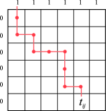
Figure 5: To determine the contribution of the element $t_{0k}$ into the element $t_{ij}$ one has to find all possible paths connecting the two elements as long as only steps down or to the right are allowed.

Summing the contributions (12) for all possible $0<k\leq j$, we obtain

$$t_{ij}=\frac{t_{0}}{2^{i+j}(i-1)!}\sum_{k=1}^{j}2^{k}\frac{(i+j-k-1)!}{(j-k)!}.$$ (13)

The final temperatures can now be found from Eqs. (9). To avoid interrupting the narrative, we move this technical step to the appendix and present here only the result,

$$t_{\rm hot}(N)=t_{0}\frac{(2N)!}{4^{N}(N!)^{2}}.$$ (14)

For a large number of splittings, $N\gg 1$, this expression can be further simplified with the help of Stirling’s approximation for the factorials,

$$N!=\sqrt{2\pi N}\,(N/e)^{N},$$ (15)

leading to the approximation (10). The curves in Fig. 6 show the accuracy of this approximation: already for $N=5$ the expression (10) overestimates the exact result (14) by only about $2\%$.

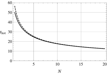
Figure 6: The solid line shows the exact $t_{\rm hot}(N)$ given by Eq. (14). The dashed line demonstrates an excellent accuracy of the approximation (10) for $N\gtrsim 5$.

We emphasize that while the final temperature of the hot water tends to zero asymptotically for $N\to\infty$, it approaches zero rather slowly. For example, it takes splitting into $N=128$ parts to cool the water to below $5\,\degree\text{C}$. At least in principle, however, we can reverse the hot and cold temperatures to any desired degree by choosing a sufficiently large $N$. (Of course, in a realistic system thermal losses to the environment would limit the efficiency of the heat exchange.)

III The continuous limit, $N\to\infty$

The complete exchange of temperatures in the limit $N\to\infty$ can also be derived from a continuum approach. As the size of the fraction $1/N$ tends to zero, the matrix element $t_{ij}$ can be viewed as a progressively smoother function of $x=i/N$ and $y=j/N$, which vary from $0$ to $1$, so that instead of a discrete matrix we have a function of two variables,

$$t_{ij}=t_{xN,yN}\equiv t_{N}(x,y),$$ (16)

which becomes continuous in the limit $N\to\infty$. In this limit the final temperature can be written as an integral:

$$t_{\rm hot}=\frac{1}{N}\sum_{j=0}^{N}t_{N}(1,j/N)\to\int\limits_{0}^{1}dy\,t_{\infty}(1,y).$$ (17)

Similarly, the final temperature of the cold water is $t_{\rm cold}=\int_{0}^{1}\,dx\,t_{\infty}(x,1).$

The function $t_{\infty}(x,y)$ can now be found from a differential equation derived from the continuum limit of the recursion relation (7). In the new notations for the function $t_{N}(x,y)$ the recursion relations are

$$t_{N}(x,y)=\frac{1}{2}\Bigl{(}t_{N}(x-{1}/{N},y)+t_{N}(x,y-{1}/{N})\Bigr{)}.$$ (18)

In the large-$N$ limit the temperature function can be expanded to the linear order in $1/N$:

$$t_{N}(x-1/N,y)=t_{N}(x,y)-\frac{1}{N}\frac{\partial t_{N}(x,y)}{\partial x}+O(1/N^{2}),$$ (19)

and similarly for the second term in Eq. (18). Disregarding the terms of the second and higher orders in $1/N$, which vanish in the leading approximation, we derive from Eq. (18) the partial differential equation

$$\frac{\partial t_{\infty}(x,y)}{\partial x}+\frac{\partial t_{\infty}(x,y)}{\partial y}=0.$$ (20)

The expressions (8) serve as the boundary conditions for this equation; in the continuous notations they become

$$t_{\infty}(0,y)=t_{0},\hskip 14.22636ptt_{\infty}(x,0)=0.$$ (21)

In order to solve Eq. (20), we first notice that any function of the difference of the two arguments satisfies it identically:

$$t_{\infty}(x,y)=f(x-y).$$ (22)

Second, from the basic theory of differential equations it is known that a general solution of a linear partial differential equation contains one and only one arbitrary function (similarly to how an ordinary linear differential equation contains one arbitrary constant).

It is now clear that both the equation and its boundary conditions will be satisfied by a solution proportional to the Heaviside step function,

$$t_{\infty}(x,y)=t_{0}\Theta(x-y),\hskip 14.22636pt\Theta(z)=\left\{\begin{array}[]{ll}1,&z>0,\\ 0,&z<0.\end{array}\right.$$ (23)

Note that this solution is not well defined at coincident arguments. In this somewhat special case we need to impose manually that $t_{\infty}(1/2,1/2)=t_{0}/2$, to reflect the corresponding property of the diagonal matrix elements for any finite $N$. This behavior is reminiscent of the Fermi-Dirac distribution, which is step-like at zero temperature but whose value is $1/2$ right at the chemical potential for any nonzero temperature.LL

From the step-like character of the solution (23) the complete temperature reversal becomes quite obvious: the ultimate temperature of the hot water is $t_{\rm hot}(\infty)=t_{0}\int_{0}^{1}dy\,\Theta(0-y)=0$.

IV What about the Second Law of thermodynamics?

The complete reversal of temperatures in the $N\to\infty$ limit is a surprising result that seems paradoxical at first glance. Indeed, the return of the closed system to the initial state—essentially the outcome in our case—is a signature of a reversible process. But thermal equilibration between objects with temperatures that differ by a non-infinitesimal amount is expected to be irreversible. Clearly that is not what happens here, even though the difference in temperatures is large.

The paradox is resolved if one notices that the conventional reasoning applies only to large bodies. When the objects themselves are infinitesimal, reversibility turns out to be possible even for nonzero differences in temperatures.

To illustrate this, let us look at what happens to the entropy of the system. We denote by $C_{0}$ the heat capacity of the whole amount of each water. When the temperature of the water (cold or hot) changes from some initial $T_{i}$ to a final $T_{f}$, its entropy changes by LL

$$\Delta S=C_{0}\int_{T_{i}}^{T_{f}}\frac{dT}{T}=\frac{C_{0}}{N}\ln{\frac{T_{f}}{T_{i}}}.$$ (24)

We emphasize that $T$ denotes the thermodynamic temperature, $T=T_{0}+t$, with $T_{0}=273$ K in our case.

The initial temperatures of the hot and cold waters are $T_{0}+t_{0}$ and $T_{0}$, respectively. At the end of the heat exchange, the temperature of the “hot” water will go down to $T_{0}+t_{\rm hot}$ while the “cold” water’s will rise to $T_{0}+t_{0}-t_{\rm hot}$. The total increase of the system’s entropy will thus be

$$\Delta S_{\rm tot}=C_{0}\left(\ln\frac{T_{0}+t_{\rm hot}}{T_{0}}+\ln\frac{T_{0}+t_{0}-t_{\rm hot}}{T_{0}+t_{0}}\right).$$ (25)

Because for large $N$ the value $t_{\rm hot}(N)\ll T_{0}$, one can expand the arguments of the logarithms using $\ln(1+x)\approx x$, and then simplify the result with the help of Eq. (10):

$$\Delta S_{\rm tot}(N)\approx C_{0}\left(\frac{t_{\rm hot}(N)}{T_{0}}-\frac{t_{\rm hot}(N)}{T_{0}+t_{0}}\right)$$

$$= \frac{C_{0}t_{0}}{T_{0}(T_{0}+t_{0})}t_{\rm hot}(N)\approx\frac{C_{0}}{\sqrt{\pi N}}\frac{t_{0}^{2}}{T_{0}(T_{0}+t_{0})}.$$ (26)

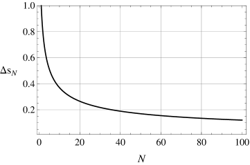
Figure 7: The total entropy change for $N$ splittings, relative to the entropy produced when the waters are brought into contact without splittling, $\Delta s_{N}=\Delta S_{\rm tot}(N)/\Delta S_{\rm tot}(1)$, as determined by Eq. (25).

Figure 7 illustrates the how the net increase in entropy, Eq. (25), depends on $N$. The total change in entropy vanishes in inverse proportion to the square root of the number of parts. Note that Eq. (IV) proves reversibility in the limit of large $N$ in a strict mathematical senseTho : for any pre-assigned $\Delta\tilde{S}$, no matter how small, there is a number $\tilde{N}$ such that for $N>\tilde{N}$ the entropy increase will be less than the pre-assigned value: $\Delta S(N)<\Delta\tilde{S}$.

It is instructive to interpret Eq. (IV) in qualitative terms. When the first element of cold water equilibrates with the first element of hot water, the temperature difference is large and the entropy increases by the maximum amount, $\sim C_{0}/N$. The resulting warming of cold water and cooling of hot water ensures that, as further elements are brought into contact, the temperature differences decrease. This makes subsequent contacts less “efficient” producers of entropy. As formula (25) suggests, by the order of magnitude, roughly $\sim\sqrt{N}$ contacts generate the maximum entropy, $\sim C_{0}/N$, meaning that the total entropy increase is of the order $\sim C_{0}/\sqrt{N}$, and vanishes in the limit of large $N$.

V Conclusions

A complete temperature reversal occurs when two bodies are split into infinitesimally small parts and brought in thermal contact sequentially. This example illustrates a type of reversible process that is less familiar than the well-known scenario. In that scenario one allows the bodies to have arbitrary size but imposes the condition that their temperatures differ by an infinitesimal amount. In the current illustration, to the contrary, the temperature differences can be arbitrary, but the bodies must be split into infinitesimal parts.

Needless to say, the analysis of this paper is subject to the usual thermodynamic restrictions. First, we have assumed that it is possible to neglect thermal losses to other bodies and to the environment (via thermal radiation, for example). Second, by “infinitesimal” parts we mean amounts of the material that are still large enough to contain many microscopic particles; the parts are thus infinitesimal only in the usual thermodynamic sense.

On the other hand, the assumption of the temperature-independent specific heat of water, while convenient, is not crucial. Even when this requirement is relaxed, the complete temperature reversal still occurs. Instead of the recurrence condition (7), one has to satisfy the condition of energy conservation. More exactly, if the heat exchange occurs at a constant pressure $P$, one has to require the conservation of the enthalpy $H(T,P)$ before and after each thermal contact:

$$2H(T_{ij},P)=H(T_{i-1\,j},P)+H(T_{i\,j-1},P).$$ (27)

Repeating now the arguments for the limit of $N\to\infty$ developed at the end of the previous section, we obtain the continuous version of Eq. (27):

$$\frac{\partial H(T,P)}{\partial T}\left(\frac{\partial T_{\infty}(x,y)}{\partial x}+\frac{\partial T_{\infty}(x,y)}{\partial y}\right)=0.$$ (28)

The derivative $\partial H/\partial T$ is the entropy, which is never zero for any nonzero $T$. As a result, the temperature function $T(x,y)$ satisfies exactly the same equation as in the case of constant specific heat. Correspondingly, this equation has the same solution (23) leading to the same conclusion of complete temperature reversal.

From a practical standpoint, the principle discussed in this paper can be realized when heat is transferred between two fluids through a dividing wall that prevents them from mixing—a design known as a recuperator or direct-transfer heat exchanger.exchanger One obvious factor limiting the efficiency of such an exchanger is the heat flow between different parts of each liquid, which results in “premature” thermalization, excluded in our idealized scheme.

*

Appendix A Derivation of Eq. (14)

To prove our final result (14) for an arbitrary number of parts $N$, we rewrite Eq. (13) in a slightly simpler form by replacing the summation variable $k$ with the new index $l=j-k$:

$$t_{ij}=\frac{t_{0}}{2^{i}(i-1)!}\sum_{l=0}^{j-1}\frac{(i+l-1)!}{2^{l}l!}.$$ (29)

A helpful identity follows from this formula and the second of the properties (11). Substituting $i=j=N+1$ into Eq. (29), we obtain that for any $N$,

$$\sum_{l=0}^{N}\frac{(N+l)!}{2^{l}\,l!}=2^{N}N!.$$ (30)

Having determined all elements of the matrix $t_{ij}$, we can now calculate the final temperature $t_{\rm hot}(N)$. As explained in the main text, it is given by the average of the first $N$ elements of $N$th row (see Eq. (9)),

$$t_{\rm hot}(N)=\frac{t_{0}}{2^{N}N!}\sum_{j=1}^{N}\sum_{l=0}^{j-1}\frac{(N+l-1)!}{2^{l}l!}.$$ (31)

Because the expression inside the summations depends on $l$ but not on $j$, it is convenient to perform the summation over $j$ first. To do so, we replace

$$\sum_{j=1}^{N}\sum_{l=0}^{j-1}\to\sum_{l=0}^{N-1}\sum_{j=l+1}^{N}.$$ (32)

The meaning of the change of the order of the summations is illustrated in Fig. 8. It is quite analogous to the reversal of the order of multiple integrations in standard calculus.

The $j$ summation now simply yields the total number of terms in the sum, $N-l$:

$$t_{\rm hot}(N)=\frac{t_{0}}{2^{N}N!}\sum_{l=0}^{N-1}\frac{(N-l)(N+l-1)!}{2^{l}l!}.$$ (33)

Now we must evaluate the remaining sum over $l$, which we abbreviate as $s_{N}$. The first step is to separate the two terms in the difference $N-l$:

$$s_{N}= \sum_{l=0}^{N-1}\frac{(N-l)(N+l-1)!}{2^{l}l!}$$

$$= N\sum_{l=0}^{N-1}\frac{(N+l-1)!}{2^{l}l!}-\sum_{l=1}^{N-1}\frac{(N+l-1)!}{2^{l}(l-1)!}.$$ (34)

Note that in the last term the summation begins at $l=1$, because of the (canceled) factor of $l$ in the numerator. The first term on the right-hand side of Eq. (A) is of the form of the sum in the relation (30) and is equal to $2^{N-1}N!$, while the last term in Eq. (A) can be brought into a similar form by the substitution $l=k+1$:

$$s_{N}=2^{N-1}N!-\frac{1}{2}\sum_{k=0}^{N-2}\frac{(N+k)!}{2^{k}k!}.$$ (35)

The remaining sum has almost the same form as the sum in the relation (30), except it lacks the two largest terms. Those terms can be subtracted explicitly:

$$s_{N}=2^{N-1}N!-\frac{1}{2}\left(2^{N}N!-\frac{(2N)!}{2^{N}N!}-\frac{(2N-1)!}{2^{N-1}(N-1)!}\right).$$ (36)

The first term inside the parenthesis cancels with the term outside, while the remaining two terms are easily verified to be equal to each other. Therefore, we obtain

$$s_{N}=\frac{(2N)!}{2^{N}N!}.$$ (37)

Replacing the sum in Eq. (33) with this expression, we obtain our main result (14).

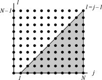
Figure 8: The summation in Eq. (31) is performed over the points belonging to the shaded triangle. It can be done in two equivalent ways, with the summations over $l$ or $j$ performed first, as prescribed by Eq. (32).

In principle, this should complete our solution. The only remaining concern is the validity of relation (30), which we obtained in an essentially “empirical” way, by observing that all diagonal components of the temperature matrix are equal to $1/2$. We now prove this relation rigorously.Raikh

Consider the sum

$$Z_{N}=\sum_{l=0}^{N}\frac{(N+l)!}{2^{l}l!},$$ (38)

and let us express the value $Z_{N+1}$ via $Z_{N}$:

$$Z_{N+1} = \sum_{l=0}^{N+1}\frac{(N+l+1)!}{2^{l}l!}=\sum_{l=0}^{N+1}\frac{(N+l+1)(N+l)!}{2^{l}l!}$$ (39)

$$= (N+1)\sum_{l=0}^{N+1}\frac{(N+l)!}{2^{l}l!}+\sum_{l=1}^{N+1}\frac{(N+l)!}{2^{l}(l-1)!}.$$

In the first sum we note that all the terms with the exception of the last one with $l=N+1$ combine into $Z_{N}$. In the second sum we replace $l=k+1$:

$$Z_{N+1}=(N+1)\left(Z_{N}+\frac{(2N+1)!}{2^{N+1}(N+1)!}\right)$$

$$+\frac{1}{2}\sum_{k=0}^{N}\frac{(N+k+1)!}{2^{k}k!}.$$ (40)

The last sum almost adds up to $Z_{N+1}$, but this time it lacks the $k=N+1$ term, which can then be explicitly subtracted from $Z_{N+1}$:

$$Z_{N+1}= (N+1)\left(Z_{N}+\frac{(2N+1)!}{2^{N+1}(N+1)!}\right)$$

$$+\frac{1}{2}\left(Z_{N+1}-\frac{(2N+2)!}{2^{N}(N+1)!}\right).$$ (41)

The two terms with the factorials exactly cancel each other. The remaining terms yield the identity

$$Z_{N+1}=2(N+1)Z_{N}.$$ (42)

Together with the initial condition $Z_{0}=1$, this recurrence relation gives $Z_{N}=2^{N}N!$, thus proving Eq. (30).

References

- (1) P. V. Makovetskiy, Look at the Root! (Nauka, Moscow, 1984).
- (2) R. K. Shah and D. P. Sekulić, Fundamentals of Heat Exchanger Design (Wiley, Hoboken, 2003).
- (3) The heat capacity of water at ambient pressure varies by less than 1%: it decreases (in J g-1 K-1) from 4.218 at to 4.178 at and then increases again to 4.216 at ; N. S. Osborne, H. F. Stimson, and D. C. Ginnings, “Measurements of Heat Capacity and Heat of Vaporization of Water in the Range to ”, J. Res. Nat. Bur. Stand. 23, 197–260 (1939).
- (4) L. D. Landau and E. M. Lifshitz, Statistical Physics (Butterworth-Heinemann, Oxford, 1980).
- (5) M. Samiullah, “What is a reversible process?,” Am. J. Phys. 75 (7), 608–609 (2007).
- (6) R. Rechtman, “An adiabatic reversible process,” Am. J. Phys. 56 (12), 1104–1105 (1988).
- (7) R. Battino, S. E. Wood, and A. G. Williamson, “On the importance of ideality,” J. Chem. Educ. 78 (10), 1364 (2001).
- (8) M. G. Calkin and D. Kiang, “Entropy change and reversibility,” Am. J. Phys. 51 (1), 78–79 (1983).
- (9) V. K. Gupta, G. Shanker, and N. K. Sharma, “Reversibility and step processes: an experiment for the undergraduate laboratory,” Am. J. Phys. 52 (10), 945–947 (1984).
- (10) W. L. McLean, “Irreversibility in step processes: some comments,” Am. J. Phys. 53 (8), 780–781 (1985).
- (11) F. Heinrich, “Entropy change when charging a capacitor: a demonstration experiment,” Am. J. Phys. 54 (8), 742–744 (1986).
- (12) E. N. Miranda, “When an irreversible cooling (or heating) becomes reversible,” Eur. J. Phys. 21 (3), 239–243 (2000).
- (13) N. C. Craig and E. A. Gislason, “First law of thermodynamics: irreversible and reversible processes,” J. Chem. Educ. 79 (2), 193–200 (2002).
- (14) J. Anacleto, J. M. Ferreira, and A. A. Soares, “When an adiabatic irreversible expansion or compression becomes reversible,” Eur. J. Phys. 30 (3), 487–495 (2009).
- (15) J. Anacleto and J. M. Ferreira, “Minimizing the generation of entropy: which sequence of reservoirs to choose,” Eur. J. Phys. 31 (1), L1–L4 (2010).
- (16) J. S. Thomsen and H. C. Bers, “The reversible process: A zero-entropy production limit,” Am. J. Phys. 64 (5), 580–583 (1996).
- (17) M. Raikh, private communication.