Reduced Modeling of Unknown Trajectories

Abstract

This paper deals with model order reduction of parametrical dynamical systems. We consider the specific setup where the distribution of the system’s trajectories is unknown but the following two sources of information are available: (i) some “rough” prior knowledge on the system’s realisations; (ii) a set of “incomplete” observations of the system’s trajectories. We propose a Bayesian methodological framework to build reduced-order models (ROMs) by exploiting these two sources of information. We emphasise that complementing the prior knowledge with the collected data provably enhances the knowledge of the distribution of the system’s trajectories. We then propose an implementation of the proposed methodology based on Monte-Carlo methods. In this context, we show that standard ROM learning techniques, such e.g., Proper Orthogonal Decomposition or Dynamic Mode Decomposition, can be revisited and recast within the probabilistic framework considered in this paper. We illustrate the performance of the proposed approach by numerical results obtained for a standard geophysical model.

1 Introduction

In many fields of Sciences, one is interested in studying the spatio-temporal evolution of a state variable characterised by a differential equation. Numerical discretisation in space and time leads to parameterised high-dimensional systems of equations of the form:

$$\left\{\begin{aligned} &x_{t}=f_{t}(x_{t-1},\theta),\\ &x_{1}=g({\theta}),\end{aligned}\right.\vspace{-0.cm}$$ (1)

where $x_{t}\in\mathds{R}^{n}$ is the state variable, ${\theta}\in\Theta$ denotes some parameters and $f_{t}:\mathds{R}^{n}\times\Theta\to\mathds{R}^{n}$, $g:\Theta\to\mathds{R}^{n}$. Because (1) may correspond to very high-dimensional systems, computing a trajectory $\{x_{t}\}_{t=1}^{T}$ may lead to unacceptable computational burdens in some applications.

As a response to this bottleneck, reduced-order models (ROMs) aim at providing “good” approximations of the trajectories of (1) (in some particular regimes of interest) via strategies only requiring significantly-reduced computational resources. Among the most familiar reduction techniques, let us mention Galerkin projection using proper orthogonal decomposition (POD) 9780511622700 or reduced basis Quarteroni2011Certified , low-rank dynamic mode decomposition (DMD) Chen12 ; HeasHerzet16 ; Jovanovic12 , second-order nonlinear operator approximation peherstorfer2016data , balanced truncation Antoulas2005Overview or Taylor expansion ZAMM:ZAMM19830630105 .

All the techniques mentioned above presuppose (explicitly or implicitly) the knowledge of the trajectories that the ROM should accurately approximate. In many contributions, such a knowledge is characterised by the (so-called) solution manifold defined as

$$\mathcal{M}=\{\mathbf{x}=(x_{1}\cdots x_{T})\in\mathds{R}^{n\times T}:\mbox{$\mathbf{x}$ obeys \eqref{eq:model_init} for some $\theta\in\Theta$}\},$$ (2)

see e.g., 2015arXiv150206797C . In this paper, we consider a slightly more general setting by assuming that the set of trajectories to reduce are specified by a probability density on $\mathbf{x}$, say $p_{\mathbf{X}}$. Unlike the standard formulation (2), density $p_{\mathbf{X}}$ then provides information on both the set of trajectories of interest (which corresponds to $p_{\mathbf{X}}\neq 0$) and their probability of occurence.

Unfortunately, in practice a precise knowledge of $p_{\mathbf{X}}$ is usually not available. In this paper, we thus address the following question: how to build a good ROM for the trajectories specified by $p_{\mathbf{X}}$ when only a rough knowledge of latter density is available but some partial observations of the trajectories are available? More specifically, we will assume that we have the following two sources of information at our disposal in the ROM construction process:

• a surrogate density $\tilde{p}_{\mathbf{X}}$: this density gathers all the information the practitioners may have about the system of interest. This density is very general in the sense it can be of any form and it does not need to satisfy any particular constraints. For example, one may know that the trajectories of interest obey (1) for some parameters included in the set $\tilde{\Theta}$. However, the true parameter set $\Theta$ and the distribution of $\theta$ over this set may be unknown. In this case, the surrogate density $\tilde{p}_{\mathbf{X}}$ could for example be defined via (1) by using a uniform distribution on $\theta$ over $\tilde{\Theta}$.

• incomplete observations on the target trajectories: we assumed that “incomplete” observations of the trajectories are available; these observations, say ${\mathbf{y}}$, are supposed to obey a known conditional model $p_{\mathbf{Y}|\mathbf{X}}$. The term “incomplete” refers to the fact a realisation $\mathbf{x}$ of $p_{\mathbf{X}}$ cannot be unequivocally recovered from its observation $\mathbf{y}$ by inverting the observation model. This situation occurs for instance when only a subset of components of $\mathbf{x}$ are observed or when the observations are corrupted by some noise. As an applicative example, in geophysics, meteorological sensors only provide low-resolution and noisy observations of the atmosphere state.

The main goal of this paper is therefore to propose a methodology taking benefit from these two sources of information to build a “good” ROM for trajectories distributed according to $p_{\mathbf{X}}$.

Before describing the contributions of this paper, we provide an overview of some state-of-the-art methodologies dealing with the problem of ROM construction from incomplete observations. The first contribution dealing with this type of problem is the “Gappy POD” technique proposed by Everson and Sirovich in Everson1995KarhunenLoeve . The authors propose to construct an approximation subspace for trajectories distributed according to $p_{\mathbf{X}}$ relying on the observed components of $\mathbf{x}$. However, this method releases poor ROM approximations as soon as some directions of the space embedding the trajectories of interest are never observed Gunes2006Gappy . This is for example the case when these trajectories are incompletely observed through the same observation model.

In order to circumvent this issue, recent works combine an observation model with a surrogate density, in the case of the reduction of a static high-dimensional system. On the one hand, several authors propose this observation and prior knowledge combination in a noise-free deterministic setting. In NME:NME4747 , the authors suggest to iteratively enrich the ROM by using point-wise estimates obtained from linear observations and a surrogate model. In HerzetHeasDremeau16 , the authors propose to refine this approach by including the uncertainty inherent to the point-wise estimates in the reduction process. Stable recovery guarantees are also provided from a worst-case perspective. On the other hand, several works have investigated the context of combining noisy observations with a probabilistic prior. The methodologies naturally rely in this case on posterior probabilities CuiEtAl2014 ; CuiMarzoukWillcox2014 ; SpantiniEtAl2015 . More precisely, in CuiMarzoukWillcox2014 , the author feed a reduced-basis technique with samples of the posterior. In CuiEtAl2014 ; SpantiniEtAl2015 , an optimal low-dimensional subspace projection of the posterior distribution is inferred based on its local Gaussian structure.

In this paper, we propose a general data-driven methodology for the reduction of parametric dynamical systems, exploiting incomplete observations. The proposed procedure exploits the two sources of information mentioned previously, namely: (i) a surrogate probabilistic characterisation of the trajectories of interest, (ii) incomplete observations of these trajectories. The proposed ROM construction relies on the minimisation of the expectation of a bound on the error between the true and reduced trajectories. The expectation relies on a new data-enhanced surrogate density, say $\hat{p}_{\mathbf{X}}$, inferred from the initial surrogate $\tilde{p}_{\mathbf{X}}$ and the partial observations. An approximated solution to this minimisation problem is efficiently computed using Monte-Carlo (MC) and Sequential Monte-Carlo (SMC) techniques. The proposed approach relies on the following assumptions:

• stability of ROM inference when using the surrogate $\tilde{p}_{\mathbf{X}}$ in place of $p_{\mathbf{X}}$,

• tightness of the error bound,

• accuracy of the expectation approximation by MC and SMC techniques.

These properties are discussed and empirically assessed in the context of our numerical simulations. The present work complements and generalises the works NME:NME4747 ; HerzetHeasDremeau16 ; CuiEtAl2014 ; CuiMarzoukWillcox2014 ; SpantiniEtAl2015 in two main respects: it proposes a methodology extending these works to the case of dynamical systems; it provides a Bayesian framework generalising any standard ROM construction to the setup where trajectories to be reduced are not fully known.

The rest of this paper is organised as follows. Section 2 first introduces the target problem and presents its surrogate analog. Section 3 then discusses implementation issues and the MC simulation techniques used to obtain a tractable method. Section 4 continues by detailing the particularisation of this methodology to the context of Galerkin projections or low-rank linear approximations. The ability of the method to take into account uncertainty is discussed at the end of this section. A numerical evaluation of the proposed methodology is exposed in Section 5 and conclusions are finally drawn in a last section.

We will use in what follows some notations. Random vectors will be denoted by uppercase letters (as $X$) and their realisations by lowercase letters (as $x$). Boldface letters (as $\mathbf{x}$) will indicate matrices, and will be uppercase (as $\mathbf{X}$) for random matrices. $p_{\mathbf{X}}$ will refer to the probability density of $\mathbf{X}$. When there is no ambiguity, the density subscript will be omitted to lighten notations, i.e., $p_{\mathbf{X}}(\mathbf{x})=p(\mathbf{x})$. The symbol $\|\cdot\|_{F}$ and $\cdot^{\intercal}$ will respectively refer to the Frobenius norm and the transpose operator; $\mathbf{i}_{k}$ will denote the $k$-dimensional identity matrix. The definition of the Kullback-Leibler distance between two densities $p_{\mathbf{X}}$ and $\tilde{p}_{\mathbf{X}}$ is

$$\textrm{KL}(p_{\mathbf{X}},\tilde{p}_{\mathbf{X}})=\int p({\mathbf{x}})\log\frac{p({\mathbf{x}})}{\tilde{p}({\mathbf{x}})}d{\mathbf{x}}.$$

2 Target and Surrogate Problems

In this section, we describe the main elements characterising our ROM construction problem. We first define the performance criterion that the ROM should ideally optimise when the target density $p_{\mathbf{X}}$ is known. We then discuss how to modify this target problem when only a surrogate density $\tilde{p}_{\mathbf{X}}$ is known but some incomplete observations ${\mathbf{y}}$ of the realisations of $p_{\mathbf{X}}$ are available.

The model-order reduction problem can essentially be formulated as follows: for any choice of $\theta\in\Theta$, find an (easily-computable) approximation ${\tilde{\mathbf{x}}}$ of ${\mathbf{x}}$, where ${\mathbf{x}}$ is specified by (1). Most ROM techniques for dynamical models encountered in the literature impose that ${\tilde{\mathbf{x}}}$ obey a recursion of the form:

$$\left\{\begin{aligned} &\tilde{x}_{t}=\tilde{f}_{t}(\tilde{x}_{t-1},\theta,\mathbf{u}),\\ &\tilde{x}_{1}=\tilde{g}(\theta,\mathbf{u}),\end{aligned}\right.$$ (3)

where $\tilde{f}_{t}:\ \mathds{R}^{n}\times\Theta\times\mathcal{U}\to\mathds{R}^{n}$ and $\tilde{g}:\Theta\times\mathcal{U}\to\mathds{R}^{n}$ are some functions specifying the ROM via the choice of parameters $\mathbf{u}\in\mathcal{U}$. The nature of $\tilde{f}_{t}$, $\tilde{g}$ and $\mathbf{u}$ depends on the family of ROMs one considers. We give two examples of choices for $\tilde{f}_{t}$, $\tilde{g}$ and $\mathbf{u}$ in Sections 4.1 and 4.2. For now, the only ingredient the reader should keep in mind is that, given a family of reduced models, the ROM is fully characterised by the choice of the parameters $\mathbf{u}\in\mathcal{U}$.

In this respect, we will assume hereafter that an ideal choice for $\mathbf{u}$ is given by

$$\mathbf{u}^{\star}=\operatorname*{arg\,min}_{\mathbf{u}\in\mathcal{U}}\Biggl{\{}\int p({\mathbf{x}})\|\mathbf{x}-\tilde{\mathbf{x}}(\mathbf{u})\|_{F}^{2}\,d{\mathbf{x}}\Biggr{\}},$$ (4)

that is, the choice of the ROM parameters should be such that they minimise the mean square approximation error over the target density $p_{\mathbf{X}}$. Here, the notation $\tilde{\mathbf{x}}(\mathbf{u})$ refers to the fact $\tilde{\mathbf{x}}$ is a function of $\mathbf{u}$. Note that it is also a function of parameter $\mathbf{x}$, since $\tilde{\mathbf{x}}$ depends on $\theta$ which is itself related to $\mathbf{x}$ through the constraint (1). Unfortunately, when $p_{\mathbf{X}}$ is unknown, evaluating $\mathbf{u}^{\star}$ according to (4) is not possible. One possible option to solve this problem may be to substitute $p_{\mathbf{X}}$ in (4) by its surrogate density $\tilde{p}_{\mathbf{X}}$, that is

$$\mathbf{u}^{\star}=\operatorname*{arg\,min}_{\mathbf{u}\in\mathcal{U}}\Biggl{\{}\int\tilde{p}({\mathbf{x}})\|\mathbf{x}-\tilde{\mathbf{x}}(\mathbf{u})\|_{F}^{2}\,d{\mathbf{x}}\Biggr{\}}.$$ (5)

This formulation does however not take into account the possible presence of partial observations ${\mathbf{y}}$ of the realisations ${\mathbf{x}}$ following $p_{\mathbf{X}}$. In this paper, we thus propose the following alternative surrogate problem:

$$\mathbf{u}^{\star}=\operatorname*{arg\,min}_{\mathbf{u}\in\mathcal{U}}\Biggl{\{}\int\hat{p}({\mathbf{x}})\|\mathbf{x}-\tilde{\mathbf{x}}(\mathbf{u})\|_{F}^{2}\,d{\mathbf{x}}\Biggr{\}},$$ (6)

where $\hat{p}_{\mathbf{X}}$ is defined as

$$\hat{p}({\mathbf{x}})=\int\hat{p}({\mathbf{x}}|{\mathbf{y}})p({\mathbf{y}})\,d{\mathbf{y}},$$ (7)

with

$$\hat{p}({\mathbf{x}}|{\mathbf{y}})=\frac{p({\mathbf{y}}|{\mathbf{x}})\tilde{p}({\mathbf{x}})}{\int p({\mathbf{y}}|{\mathbf{x}}^{\prime})\tilde{p}({\mathbf{x}}^{\prime})\,d{\mathbf{x}}^{\prime}}.$$ (8)

We note that $\hat{p}_{\mathbf{X}}$ obeys the standard relationship between a joint density and its marginal. More specifically, we have from elementary probability theory that $p({\mathbf{x}})=\int p({\mathbf{x}},{\mathbf{y}})\,d{\mathbf{y}}=\int p({\mathbf{x}}|{\mathbf{y}})p({\mathbf{y}})\,d{\mathbf{y}}$. Since $p_{\mathbf{X}|\mathbf{Y}}$ depends on $p_{\mathbf{X}}$ and is therefore unknown, we propose to substitute this quantity by the surrogate posterior $\hat{p}_{\mathbf{X}|\mathbf{Y}}$ defined in (8). Similarly, the latter surrogate verifies the standard definition of the posterior probability $p_{\mathbf{X}|\mathbf{Y}}$ with the difference that the target prior $p_{\mathbf{X}}$ has been replaced by $\tilde{p}_{\mathbf{X}}$.

On top of these intuitive arguments motivating the definition of $\hat{p}_{\mathbf{X}}$, the following result provide a theoretical justification to (7)-(8):

Proposition 1

Let $\hat{p}_{\mathbf{X}}$ be defined as in (7)-(8). Then we have

$$\mathrm{KL}(p_{\mathbf{X}},\hat{p}_{\mathbf{X}})\leq \mathrm{KL}(p_{\mathbf{X}},\tilde{p}_{\mathbf{X}})-\mathrm{KL}(p_{\mathbf{Y}},\hat{p}_{\mathbf{Y}}),$$ (9)

where

$$\hat{p}({\mathbf{y}})=\int p({\mathbf{y}}|{\mathbf{x}})\tilde{p}({\mathbf{x}})\,d{\mathbf{x}}.$$ (10)

Proof: The result is a consequence of the following inequalities:

$$\mathrm{KL}(p(\mathbf{x}),p^{(k)}(\mathbf{x})) \stackrel{{\scriptstyle(a)}}{{=}}\int p({\mathbf{x}})\Bigl{(}\log p({\mathbf{x}})-\log\hat{p}({\mathbf{x}})\Bigr{)}d{\mathbf{x}},$$

$$\stackrel{{\scriptstyle(b)}}{{=}}\int p({\mathbf{x}})\Bigl{(}\log p({\mathbf{x}})-\log\tilde{p}({\mathbf{x}})-\log\int p(\mathbf{y}|\mathbf{x})\frac{p(\mathbf{y})}{\hat{p}(\mathbf{y})}d\mathbf{y}\Bigr{)}d{\mathbf{x}},$$

$$\stackrel{{\scriptstyle(c)}}{{\leq}}\int p({\mathbf{x}})\Bigl{(}\log p({\mathbf{x}})-\log\tilde{p}({\mathbf{x}})-{\int p(\mathbf{y}|\mathbf{x})\log\frac{p(\mathbf{y})}{\hat{p}(\mathbf{y})}}d\mathbf{y}\Bigr{)}d{\mathbf{x}},$$

$$\stackrel{{\scriptstyle(d)}}{{=}}\int p(\mathbf{x})\Bigl{(}\log p(\mathbf{x})-\log\tilde{p}(\mathbf{x})\Bigr{)}d{\mathbf{x}}-\int p(\mathbf{y})\Bigl{(}\log p(\mathbf{y})-\log\hat{p}(\mathbf{y})\Bigr{)}d\mathbf{y},$$

where $(a)$ follows from the definition of the Kullback-Leibler distance, $(b)$ from the definition of $\hat{p}_{\mathbf{X}}$ in (7)-(8), $(c)$ is a consequence of the Jensen’s inequality, and $(d)$ follows from $\int p({\mathbf{y}}|{\mathbf{x}})p({\mathbf{x}})\,d{\mathbf{x}}=p({\mathbf{y}})$. $\square$

The operational meaning of Proposition 1 is as follows: as far as the Kullback-Leibler distance is considered, the approximation of $p_{\mathbf{X}}$ by $\hat{p}_{\mathbf{X}}$ is at least as good as the approximation of $p_{\mathbf{X}}$ by our surrogate $\tilde{p}_{\mathbf{X}}$. Moreover, when $\mathrm{KL}(p_{\mathbf{Y}},\hat{p}_{\mathbf{Y}})>0$, the proposed approximation $\hat{p}_{\mathbf{X}}$ leads to a strict improvement of the initial surrogate $\tilde{p}_{\mathbf{X}}$, that is $\mathrm{KL}(p_{\mathbf{X}},\hat{p}_{\mathbf{X}})<\mathrm{KL}(p_{\mathbf{X}},\tilde{p}_{\mathbf{X}})$. On the one hand, $\hat{p}_{\mathbf{Y}}$ can be understood as the distribution that the observations should obey if the state variable ${\mathbf{x}}$ was distributed according to $\hat{p}_{\mathbf{X}}$. On the other hand, $p_{\mathbf{Y}}$ corresponds to the actual distribution of the collected observations $\mathbf{y}$. Since $\mathrm{KL}(p_{\mathbf{Y}},\hat{p}_{\mathbf{Y}})=0$ if and only if $p_{\mathbf{Y}}({\mathbf{y}})=\hat{p}_{\mathbf{Y}}({\mathbf{y}})$ (almost everywhere), we see that $\hat{p}_{\mathbf{X}}$ leads to a strict improvement over $\tilde{p}_{\mathbf{X}}$ as soon as the empirical distribution of the collected data deviates from the surrogate $\hat{p}_{\mathbf{Y}}$.

We can notice that $\hat{p}_{\mathbf{X}}$ depends on the observations ${\mathbf{y}}$ via the distribution $p_{\mathbf{Y}}$ in (7). The precise knowledge of $p_{\mathbf{Y}}$ is however inaccessible in most experimental setups and in order to build $\hat{p}_{\mathbf{X}}$, the practitioner can only access to a finite set of realisations of the observed random variable. We will detail in the following how $\hat{p}_{\mathbf{X}}$ is approximated from this finite set of observations.

3 Implementation Issues

The target problem exposed in the previous section is intractable directly. Its resolution will rely on several levels of approximations. They are detailed below.

3.1 MC Approximation

In practice, we are often faced to the lack of knowledge of the density $p_{\mathbf{Y}}$. Nevertheless, a practitioner may have access to a finite set of partial observations

$$\{\mathbf{y}^{(i)}\in\mathds{R}^{m\times T};\quad i=1,\cdots,D\},$$

where $m<n$, composed of realisations assumed independent and identically distributed (i.i.d.) according to the density $p_{\mathbf{Y}}$. Relying on these observations, we propose to approximate the marginalisation integral in (7) via a standard MC technique. This leads to the following approximation of the cost function in problem (6)

$$\int\hat{p}({\mathbf{x}})\|\mathbf{x}-\tilde{\mathbf{x}}(\mathbf{u})\|^{2}_{F}d\mathbf{x}\simeq\frac{1}{D}\sum_{i=1}^{D}\int\hat{p}({\mathbf{x}}|{\mathbf{y}}^{(i)})\|\mathbf{x}-\tilde{\mathbf{x}}(\mathbf{u})\|^{2}_{F}d\mathbf{x}.$$ (11)

We remark that, by introducing this MC approximation, observations ${\mathbf{y}}^{(i)}$ now appear explicitly in the ROM inference problem, on the contrary to the cost function in problem (6) which only exhibits a dependence to the unknown density $p_{\mathbf{Y}}$. It is well know that the right-hand side of equation (11) is an unbiased estimate of the left-hand side with an error variance evolving as $\mathcal{O}(D^{-1})$.

3.2 SMC Approximation

In the general case, the density $\hat{p}_{\mathbf{x}|\mathbf{y}^{(i)}}$ appearing in (11) is not closed-form and we can often not compute analytically posterior expectations. We pursue an approximation of this density for $i=1,...,D$ by an empirical measure of the form

$$\hat{p}(\mathbf{x}|{\mathbf{y}}^{(i)})\simeq\frac{1}{N}\sum_{j=1}^{N}w^{(i,j)}\delta_{\boldsymbol{\xi}^{(i,j)}}(\mathbf{x}),$$ (12)

which relies on a set of $N$ samples $\{\boldsymbol{\xi}^{(i,j)}\}_{j=1}^{N}$, weights $\{w^{(i,j)}\}_{j=1}^{N}$ with $\boldsymbol{\xi}^{(i,j)}=(\xi^{(i,j)}_{1}\cdots\xi^{(i,j)}_{T})\in\mathds{R}^{n\times T}$ and $w^{(i,j)}\in\mathds{R}_{+}$ and the Dirac measure $\delta_{\mathbf{x}}$. This leads to an approximation of the cost function in problem (6) by the weighted sum

$$\int\hat{p}(\mathbf{x}|\mathbf{y}^{(i)})\|\mathbf{x}-\tilde{\mathbf{x}}(\mathbf{u})\|_{F}^{2}d\mathbf{x}\approx\frac{1}{N}\sum_{j=1}^{N}w^{(i,j)}\|{\boldsymbol{\xi}}^{(i,j)}-\tilde{\mathbf{x}}(\mathbf{u})\|^{2}_{F},$$ (13)

and combining approximations (11) and (13), we obtain

$$\int\hat{p}({\mathbf{x}})\|\mathbf{x}-\tilde{\mathbf{x}}(\mathbf{u})\|_{F}^{2}\,d{\mathbf{x}}\simeq\frac{1}{DN}\sum_{i=1}^{D}\sum_{j=1}^{N}w^{(i,j)}\|{\boldsymbol{\xi}}^{(i,j)}-\tilde{\mathbf{x}}(\mathbf{u})\|^{2}_{F}.$$ (14)

In the case of dynamical systems, $\hat{p}_{\mathbf{X}|\mathbf{Y}}$ in (12) often exhibits a nested structure which can be sampled in a sequential manner. In particular, the surrogate density $\tilde{p}_{\mathbf{X}}$, used for defining $\hat{p}_{\mathbf{X}|\mathbf{Y}}$ in (8), often takes the form of a Markov chain defined by a transition kernel and an initial density

$$\left\{\begin{aligned} \tilde{p}(x_{t}|x_{t-1})&=\pi_{t}(x_{t},x_{t-1}),\\ \tilde{p}(x_{1})&=\eta_{1}(x_{1}),\end{aligned}\right.\vspace{-0.cm}$$ (15)

which will imply the density factorisation

$$\tilde{p}(\mathbf{x})=\eta_{1}(x_{1})\prod_{t=2}^{T}\pi_{t}(x_{t},x_{t-1}).$$ (16)

SMC techniques are particularly well suited to this context and constitute tractable methods able to compute efficiently a relevant set of $N$ samples and weights $\{\boldsymbol{\xi}^{(i,j)},w^{(i,j)}\}_{j=1}^{N}$ involved in (12). Among the variety of SMC techniques, the most known methods are sequential importance sampling or bootstrap particle filtering doucet2000sequential . These algorithms exploit an observation model admitting the factorisation

$$p_{\mathbf{Y}|\mathbf{X}}=\prod_{t=1}^{T}p_{Y_{t}|X_{t}},$$ (17)

where the random matrix $\mathbf{{Y}}=(Y_{1}\cdots Y_{T})$ gathers the observed variables at the $T$ different temporal indexes. For large $N$, approximation (13) by SMC techniques is accurate in the sense that it will yield an unbiased (or asymptotically unbiased) estimation of the posterior expectation in the case the cost function is a bounded function of $\mathbf{x}$. Moreover, under this boundedness hypothesis, the variance of the estimation error will decrease at the rate of $\mathcal{O}(N^{-1})$, see e.g., crisan2002survey . However, in the our case, the error norm $\|\mathbf{x}-\tilde{\mathbf{x}}(\mathbf{u})\|^{2}_{F}$ is in general not bounded. Although progress has been recently accomplished in this direction 2015arXiv151106196A , extending these asymptotical unbiased properties and convergence results to the case of unbounded test functions has not been done yet in the context of SMC approximations.

3.3 Practical Identification of a Minimiser

With the simplifications proposed in Sections 3.1 and 3.2, our surrogate optimisation problem takes the form:

$$\mathbf{u}^{\star} =\operatorname*{arg\,min}_{\mathbf{u}\in\mathcal{U}}\Biggl{\{}\sum_{i=1}^{D}\sum_{j=1}^{N}w^{(i,j)}\|{\boldsymbol{\xi}}^{(i,j)}-\tilde{\mathbf{x}}(\mathbf{u})\|^{2}_{F}\Biggr{\}}.$$ (18)

Unfortunately, (18) is typically a non-convex optimisation problem. Hence, designing polynomial-time optimisation procedures ensuring the identification of a global minimiser $\mathbf{u}^{\star}$ of (18) for any problem instance is usually out of reach. In order to circumvent this issue, two different approaches are usually suggested in the literature: (i) resorting to local optimisation procedures; (ii) optimising an upper bound of the cost function in (18).

The local optimisation procedures encountered in practice usually derive from iterative gradient descent methods. When the ROM approximation $\tilde{{\mathbf{x}}}(\mathbf{u})$ satisfies a recursion as (3), these methods can be efficiently implemented by using adjoint procedures, see for example Hasselmann88 ; Kwasniok96 . The drawback of local optimisation procedures is however that they are prone to converge to local optimum of the cost function. In many situations, this behavior may prevent these methods from delivering a solution close to the global minimiser $\mathbf{u}^{\star}$, leading in turn to poor reduction performance.

In order to circumvent this problem, another approach pursued in the literature consists in optimising an upper bound on the cost function, that is

$$\mathbf{u}^{\star} =\operatorname*{arg\,min}_{\mathbf{u}\in\mathcal{U}}\{J(\mathbf{u})\},$$ (19)

where $J(\mathbf{u})$ is such that

$$\sum_{i=1}^{D}\sum_{j=1}^{N}w^{(i,j)}\|{\boldsymbol{\xi}}^{(i,j)}-\tilde{\mathbf{x}}(\mathbf{u})\|^{2}_{F}\leq J(\mathbf{u})\quad\forall\mathbf{u}\in\mathcal{U}.$$ (20)

Of course, the minimisers of (19) usually differ from those of (18). Nevertheless, if the behavior of $J(\mathbf{u})$ is “not too far” from the one of $\sum_{i=1}^{D}\sum_{j=1}^{N}w^{(i,j)}\|{\boldsymbol{\xi}}^{(i,j)}-\tilde{\mathbf{x}}(\mathbf{u})\|^{2}_{F}$, one may expect the minimisers of $\eqref{eq:minupperbound}$ to be good approximations of the solutions of (18). Moreover, the numerical optimisation (19) may be far easier than the one of the initial optimisation problem (18). We will provide two instances of such scenarios in Section 4.

In the sequel, we will exclusively focus our attention on methodologies based on the optimisation of an upper bound. This is motivated by the fact that, by using this approach, several methodologies known in the reduced-model community can be revisited and extended in the probabilistic framework considered in this paper. Nevertheless, the methodologies based on local optimisation procedure could be applied in a similar way in the framework discussed in this paper.

4 Two Examples

In this section, we illustrate how the procedure presented in Section 3 particularises to two different families of ROMs. In particular, we will show that these particularisations can be seen as generalisations, in a probabilistic framework, of well-known ROM techniques, namely POD and DMD. We also discuss how they can be seen as generalisations of standard ROM constructions based on point estimates.

4.1 Galerkin Projection

The low-rank approximation called Galerkin projection of the dynamics (1) is obtained by projecting $x_{t}$’s onto a subspace spanned by the columns of some matrix $\mathbf{u}\in\mathds{R}^{n\times k}$ with orthonormal columns and where $k<n$, see e.g., quarteroni2015reduced . More precisely, it consists in a recursion

$$\left\{\begin{aligned} &z_{t}=\mathbf{u}^{\intercal}{f}_{t}(\mathbf{u}z_{t-1},\theta),\\ &z_{1}=\mathbf{u}^{\intercal}g(\theta),\end{aligned}\right.$$ (21)

defining a sequence of $k$-dimensional variables $\{z_{t}\in\mathds{R}^{k}\}_{t=1}^{T}$. Because $k<n$, system (21) is usually either tractable or efficient methods can be used to simplify computation Barrault2004667 ; chaturantabut2010nonlinear . Once recursion (21) has been evaluated, an approximation of state $x_{t}$ can simply be obtained as $\tilde{x}_{t}=\mathbf{u}z_{t}$. Recursion (21) is thus a particularisation of (3) with

$$\tilde{f}_{t}(\tilde{x}_{t-1},\theta,\mathbf{u})=\mathbf{u}\mathbf{u}^{\intercal}f_{t}(\mathbf{u}\mathbf{u}^{\intercal}\tilde{x}_{t-1},\theta),$$

$$\tilde{g}(\theta,\mathbf{u})=\mathbf{u}\mathbf{u}^{\intercal}g(\theta).$$

Setting $\tilde{f}_{t}$ and $\tilde{g}$ as above implies that (18) with the admissible set

$$\mathcal{U}=\{\mathbf{u}\in\mathds{R}^{n\times k}|\mathbf{u}^{\intercal}\mathbf{u}=\mathbf{i}_{k}\}$$ (22)

is a non-convex minimisation problem exhibiting a complex sequential structure. Unfortunately, no polynomial-time optimisation methods can ensure the identification of a global minimiser in this context. We resort instead to the optimisation of the following upper bound of the cost function in (18)

$$J(\mathbf{u})=c\sum_{i}\sum_{j}w^{(i,j)}\|{\boldsymbol{\xi}}^{(i,j)}-\mathbf{u}\mathbf{u}^{\intercal}{\boldsymbol{\xi}}^{(i,j)}\|_{F}^{2}$$ (23)

where $c>0$. Indeed, using a generalisation of Céa’s lemma to strongly monotone and Lipschitz-continuous functions Ciarlet02 , we obtain

$$\|\mathbf{x}-\mathbf{u}\mathbf{u}^{\intercal}\mathbf{x}\|^{2}_{F}\leq\|\mathbf{x}-\tilde{\mathbf{x}}(\mathbf{u})\|^{2}_{F}\leq c\,\|\mathbf{x}-\mathbf{u}\mathbf{u}^{\intercal}\mathbf{x}\|^{2}_{F}.$$ (24)

for any $\mathbf{x}\in\mathds{R}^{n\times T}$ and with the constant $c$ independent of $\mathbf{u}$. This bound is tight for small $c$, since it encloses from above and below the error norm. The upper bound in (24) is obtained under the assumption that the mapping $\mathds{R}^{n\times T}\to\mathds{R}^{n\times T},\mathbf{x}\to(x_{1},-f_{1}(x_{1})+x_{2},-f_{2}(x_{2})+x_{3},\cdots,-f_{T-1}(x_{T-1})+x_{T})$ is strongly monotone and that it is Lipschitz-continuous for bounded arguments (Ciarlet02, , Theorem 5.3.4). We remark that the optimisation of the bound (23) can be seen as a POD-like problem, where standard snapshots are substituted by weighted samples obtained by MC and SMC simulations.

Problem (19) with the upper bound (23) and the admissible set (22) admits a closed-form solution $\mathbf{u}^{\star}$. Indeed, a well-known result is that the columns of matrix $\mathbf{u}^{\star}$ are the eigenvectors of matrix $\mathbf{c}\mathbf{c}^{\intercal}$ where

$$\mathbf{c}=(\sqrt{w^{(1,1)}}\boldsymbol{\xi}^{(1,1)}\cdots\sqrt{w^{(D,N)}}\boldsymbol{\xi}^{(D,N)})\in\mathds{R}^{n\times TDN},$$

associated to its $k$ largest eigenvalues jolliffe2002principal . In practice, eigenvectors of interest can be derived from the eigen-decomposition of the smaller matrix $\mathbf{c}^{\intercal}\mathbf{c}$, see e.g., quarteroni2015reduced .

According to the convergence results of MC and SMC techniques, we also see that $\mathbf{u}^{\star}$ is an unbiased estimator of the closed-formed solution of

$$\operatorname*{arg\,min}_{\mathbf{u}\in\mathcal{U}}\,c\int\hat{p}({\mathbf{x}})\|\mathbf{x}-\mathbf{u}\mathbf{u}^{\intercal}\mathbf{x}\|_{F}^{2}\,d{\mathbf{x}}.$$ (25)

We thus have the following proposition.

Proposition 2

For any positive integer $k\leq TDN$ the eigenvectors corresponding to the $k$ largest eigenvalues of matrix $\mathbf{c}\mathbf{c}^{\intercal}$ are the columns of the solution of (19) with the upper bound (23) and the admissible set (22). Moreover, they are unbiased estimators of the columns of the matrix solving (25).

4.2 Low-Rank Linear Approximation

A low-rank linear approximation of the dynamics (1) is a particularisation of (3) to

$$\tilde{f}_{t}(\tilde{x}_{t-1},\theta,\mathbf{u})=\mathbf{u}\tilde{x}_{t-1},$$

$$\tilde{g}(\theta,\mathbf{u})=g(\theta),$$ (26)

parameterised by some matrix $\mathbf{u}\in\mathds{R}^{n\times n}$ of rank lower or equal to $k\leq n$. Let its singular value decomposition (SVD) be $\mathbf{u}=\mathbf{w}_{\mathbf{u}}\boldsymbol{\sigma}_{\mathbf{u}}\mathbf{v}_{\mathbf{u}}^{\intercal},$ with $\mathbf{w}_{\mathbf{u}},\mathbf{v}_{\mathbf{u}}\in\mathds{R}^{n\times k}$ and $\boldsymbol{\sigma}_{\mathbf{u}}\in\mathds{R}^{k\times k}$ so that $\mathbf{w}_{\mathbf{u}}^{\intercal}\mathbf{w}_{\mathbf{u}}=\mathbf{v}_{\mathbf{u}}^{\intercal}\mathbf{v}_{\mathbf{u}}=\mathbf{i}_{k}$ and $\boldsymbol{\sigma}_{\mathbf{u}}$ is diagonal. The $n$-dimensional reduced states $\{\tilde{x}_{t}\}_{t=1}^{T}$ are fully determined by the following recursion,

$$\left\{\begin{aligned} &z_{t}=(\mathbf{v}_{\mathbf{u}}\boldsymbol{\sigma}_{\mathbf{u}})^{\intercal}\mathbf{w}_{\mathbf{u}}z_{t-1},\\ &z_{2}=(\mathbf{v}_{\mathbf{u}}\boldsymbol{\sigma}_{\mathbf{u}})^{\intercal}\mathbf{w}_{\mathbf{u}}^{\intercal}g(\theta),\end{aligned}\right.$$ (27)

only involving $k$-dimensional variables. By multiplying both sides of (27) by $\mathbf{w}_{\mathbf{u}}$, we obtain low-rank approximations $\tilde{x}_{t}=\mathbf{w}_{\mathbf{u}}z_{t}$ of the $n$-dimensional states $x_{t}$ defined in (1).

Setting $\tilde{f}_{t}$ and $\tilde{g}$ as in (4.2) and the admissible set as

$$\mathcal{U}=\{\mathbf{u}\in\mathds{R}^{n\times n}|\textrm{rank}(\mathbf{u})\leq k,\|\mathbf{u}\|_{2,2}\leq\lambda\}$$ (28)

defines a non-convex problem (18) due to the low-rank constraint and the sequential structure of (4.2). The global minimiser is out of reach in this context. Here again, we choose to resort to the optimisation of the following upper bound of the cost function in (18):

$$J(\mathbf{u})=c\sum_{i=1,j=1}^{D,N}w^{(i,j)}\sum_{t=2}^{T}\|{\xi}_{t}^{(i,j)}-\mathbf{u}{\xi}_{t-1}^{(i,j)}\|^{2}_{F}$$ (29)

where $c>0$ depends on $\lambda$. Indeed, for any $\mathbf{x}\in\mathds{R}^{n\times T}$, it is shown in Appendix A.1 that the ROM error can be bounded for any $\mathbf{u}\in\mathcal{U}$ as

$$\sum_{t=2}^{T}\|x_{t}-\mathbf{u}x_{t-1}\|^{2}_{2}\leq\|\mathbf{x}-\tilde{\mathbf{x}}(\mathbf{u})\|^{2}_{F}\leq c\,\sum_{t=2}^{T}\|x_{t}-\mathbf{u}x_{t-1}\|_{2}^{2}.$$ (30)

As in the previous example, this bound is tight as long as $c$ is small since it encloses from above and below the error norm.

A reasonable condition to set $\lambda$ is that (28) includes at least the minimisers over the unconstrained domain $\{\mathbf{u}\in\mathds{R}^{n\times n}|\textrm{rank}(\mathbf{u})\leq k\}$ of the ROM error norm and of the bound (i.e., the left and right hand side of the second inequality in (30)). Appendix A.2 shows that these minimisers have a finite norm, i.e., that there exists $\lambda<\infty$ satisfying this condition. This implies that there exists $\lambda<\infty$ such that the constraint $\|\mathbf{u}\|_{2,2}\leq\lambda$ is inactive at the minima of the bound so that the constraint can be removed from the optimisation problem. Optimising (29) over (28) can in consequence be seen as a low-rank DMD-like problem, where standard snapshots are substituted by weighted samples obtained by MC and SMC simulations. The optimisation of this upper bound admits a closed-form solution as shown recently in HeasHerzet16 . Indeed, defining matrices $\mathbf{a},\mathbf{b}\in\mathds{R}^{n\times(T-1)DN}$ as

$$\mathbf{a} =(\sqrt{w^{(1,1)}}\boldsymbol{\xi}^{(1,1)}_{1:T-1}\cdots\sqrt{w^{(D,N)}}\boldsymbol{\xi}^{(D,N)}_{1:T-1}),$$

$$\mathbf{b} =(\sqrt{w^{(1,1)}}\boldsymbol{\xi}^{(1,1)}_{2:T}\cdots\sqrt{w^{(D,N)}}\boldsymbol{\xi}^{(D,N)}_{2:T}),$$

with the notations $\boldsymbol{\xi}^{(i,j)}_{\ell:m}=(\xi^{(i,j)}_{\ell}\cdots\xi^{(i,j)}_{m}),$ the optimisation problem can be rewritten in the synthetic form

$$\mathbf{u}^{\star}\in\operatorname*{arg\,min}_{\mathbf{u}\in\mathcal{U}}\|\mathbf{b}-\mathbf{u}\mathbf{a}\|^{2}_{F},$$ (31)

where $\mathcal{U}$ is defined in (28) with $\lambda=\infty$. This problem admits the closed-form solution $\mathbf{u}^{\star}=\mathbf{p}\mathbf{p}^{\intercal}\mathbf{b}\mathbf{a}^{\dagger}$, where the columns of $\mathbf{p}\in\mathds{R}^{n\times k}$ are real orthonormal eigenvectors associated to the largest eigenvalues of matrix $\mathbf{b}\mathbf{a}^{\dagger}\mathbf{a}\mathbf{b}^{\intercal}$, and where $\mathbf{a}^{\dagger}=\mathbf{v}_{\mathbf{a}}\boldsymbol{\sigma}_{\mathbf{a}}^{-1}\mathbf{w}_{\mathbf{a}}^{\intercal}$ is the Moore-Penrose pseudo-inverse of $\mathbf{a}$ (HeasHerzet16, , Theorem 3.1). We note that this solution can be efficiently computed by SVDs, as detailed in (HeasHerzet16, , Algorithm 1).

According to the convergence results of MC and SMC techniques, we remark that $\mathbf{u}^{\star}$ is an unbiased estimator of the closed-formed solution of

$$\operatorname*{arg\,min}_{\mathbf{u}\in\mathcal{U}}\,c\int\hat{p}({\mathbf{x}})\sum_{t=2}^{T}\|x_{t}-\mathbf{u}x_{t-1}\|_{2}^{2}\,d{\mathbf{x}}.$$ (32)

This yields the following proposition.

Proposition 3

For any positive integer $k\leq(T-1)DN$, $\mathbf{u}^{\star}=\mathbf{p}\mathbf{p}^{\intercal}\mathbf{b}\mathbf{a}^{\dagger}$ is a solution of (31) and an unbiased estimator of a solution of (32).

4.3 Comparison with ROM Based on Point Estimates

We show that the ROM parameter $\mathbf{u}^{\star}$ inferred in Section 4.1 or 4.2 differs from the parameter inferred relying on point estimates NME:NME4747 ; Sirovich87 . The latter approach consists in building the ROM from estimates of the state, say $\hat{{\mathbf{x}}}^{(i)}$, computed for $i=1,...,D$ by combining the received observation ${\mathbf{y}}^{(i)}$ and the surrogate $\tilde{p}_{\mathbf{X}}$. A common choice to obtain these estimates is to rely on the minimum mean square error (MMSE) estimator, i.e.,

$$\hat{{\mathbf{x}}}^{(i)}=\int\mathbf{x}\,\hat{p}(\mathbf{x}|\mathbf{y}^{(i)})\,d\mathbf{x}.$$

The parameter of a ROM based on MMSE point estimates is then obtained by solving

$$\operatorname*{arg\,min}_{\mathbf{u}\in\mathcal{U}}\Biggl{\{}\sum_{i=1}^{D}\|\hat{{\mathbf{x}}}^{(i)}-\tilde{\mathbf{x}}(\mathbf{u})\|^{2}_{F}\Biggr{\}}.$$ (33)

In what follows, we will refer to this particular choice of estimator when invoking ROM based on point estimates.

Analogously to our approach, we may obtain an unbiased (or asymptotically unbiased) approximation of the MMSE estimator using an SMC technique

$$\hat{{\mathbf{x}}}^{(i)}\simeq\frac{1}{N}\sum_{j=1}^{N}w^{(i,j)}{\boldsymbol{\xi}}^{(i,j)}.$$ (34)

Comparing (18) with the optimisation problem (33) where the $\hat{{\mathbf{x}}}^{(i)}$’s are approximated with (34), we see that our approach can be seen as a generalisation of a point estimate approach where the approximation of $\hat{p}_{\mathbf{X}|\mathbf{Y}}$ relies on $N$ particles rather than on a single one.

Let us further detail the differences between the two approaches. Note that matrix $\mathbf{c}\mathbf{c}^{\intercal}$ or matrices $\mathbf{b}\mathbf{a}^{\intercal}$ and $\mathbf{a}\mathbf{a}^{\intercal}$ introduced previously are MC and SMC approximations of matrices of the form

$$\int p(\mathbf{y})d\mathbf{y}\int\hat{p}(\mathbf{x}|\mathbf{y})\,\mathbf{x}_{1+\ell:T}\mathbf{x}_{1:T-\ell}^{\intercal}d\mathbf{x},\quad\ell\in\{0,1\},$$ (35)

where we have used the notations $\mathbf{x}_{\ell:m}=(x_{\ell}\cdots x_{m})\in\mathds{R}^{n\times(m-\ell+1)}.$ In particular, according to (11), matrices (35) are approximated in our methodology by a MC technique yielding

$$\frac{1}{D(T-\ell)}\sum_{i,t=1+\ell}^{D,T}\Biggl{(} \int\hat{p}(\mathbf{x}|\mathbf{y}^{(i)})\left(x_{t-\ell}-\hat{x}_{t-\ell}^{(i)}\right)\left(x_{t}-\hat{x}_{t}^{(i)}\right)^{\intercal}d\mathbf{x}+\hat{x}_{t-\ell}^{(i)}(\hat{x}_{t}^{(i)})^{\intercal}\Biggr{)},$$ (36)

where $\hat{x}_{t-\ell}^{(i)}$ are MMSE point estimates. Note that the first term inside the brackets is the cross-covariance relative to $\hat{p}(\mathbf{x}|\mathbf{y}^{(i)})$ of vectors $X_{t-\ell}$ and $X_{t}$, while the second term is the square of the mean of this density. ROMs based on point estimates rely only on the mean and ignore cross-covariance terms. They approximate matrices (35) by

$$\frac{1}{D(T-\ell)}\sum_{i,t=1+\ell}^{D,T}\hat{x}_{t-\ell}^{(i)}(\hat{x}_{t}^{(i)})^{\intercal}.$$ (37)

Choosing approximate matrix (37) instead of (36) may imply a poor approximation of (35). In particular, (36) and (37) will significantly differ in the case of large cross-covariances. Making a correspondence between cross-covariances and uncertainty, this suggests that the proposed method integrates uncertainty relative to point estimates in the ROM inference process.

5 Numerical Evaluation

We assess the proposed methodology with a standard physical model known as Rayleigh-Bénard convective system. After introducing the parametric partial differential equation inducing the high-dimensional system, we provide different variations of the ROM building problem. They differ from each other by their underlying probabilistic models $p_{\mathbf{X}}$, $\hat{p}_{\mathbf{X}}$ and $p_{\mathbf{Y}|\mathbf{X}}$. Based on this setup, we finally evaluate the performance of four different sampling strategies to build a ROM in our uncertain context.

5.1 The Physical Setup

We consider a Rayleigh-Bénard convective system chandrasekhar2013hydrodynamic . An incompressible fluid is contained in a bi-dimensional cell and is subject to periodic boundary conditions. The states of interest are the trajectories of the temperature and velocity fields in the cell.

We introduce the following notations to state the evolution equations: the differential operators $\nabla=(\partial_{s_{1}},\partial_{s_{2}})^{\intercal}$, $\nabla^{\perp}=(\partial_{s_{2}},-\partial_{s_{1}})^{\intercal}$ and $\Delta=\partial^{2}_{s_{1}}+\partial^{2}_{s_{2}}$ denote the gradient, the curl and the Laplacian with respect to the two spatial dimensions $(s_{1},s_{2})$; the operator $\Delta^{-1}$ is the formal representation of the inverse of $\Delta$. Convection is driven by the two following coupled partial differential equations: at any point of the unit cell $\mathbf{s}=(s_{1},s_{2})\in[0,1]^{2}$ and for any time $t\geq 1$, we have

$$\left\{\begin{aligned} \partial_{t}b(\mathbf{s},t)+\mathbf{v}(\mathbf{s},t)\cdot\nabla b(\mathbf{s},t)-\rho\Delta b(\mathbf{s},t)-\rho\nu\partial_{s_{1}}\tau(\mathbf{s},t)&=0,\\ \partial_{t}\tau(\mathbf{s},t)+\mathbf{v}(\mathbf{s},t)\cdot\nabla\tau(\mathbf{s},t)-\Delta\tau(\mathbf{s},t)-\partial_{s_{1}}\Delta^{-1}b(\mathbf{s},t)&=0,\end{aligned}\right.$$ (38)

where $\tau(\mathbf{s},t)\in\mathds{R}$ and $\mathbf{v}(\mathbf{s},t)\in\mathds{R}^{2}$ are the temperature and the velocity and where the buoyancy $b(\mathbf{s},t)\in\mathds{R}$ satisfies

$$\mathbf{v}(\mathbf{s},t)=\nabla^{\perp}\Delta^{-1}b(\mathbf{s},t).$$

The parameters $\rho$ and $\nu$ appearing in (38) have the following physical meaning. The Rayleigh number $\nu\in\mathds{R}_{+}$ controls the balance between thermal diffusion and the tendency for a packet of fluid to rise due to the buoyancy force. The Prandtl number $\rho\in\mathds{R}_{+}$ measures the relative importance of viscosity compared to thermal diffusion. These two parameters control the coupling of the buoyancy evolution with the thermal diffusion process. In particular for $\nu=0$ and/or $\rho=0$, the system is decoupled in the sense that the evolution of buoyancy is independent of temperature.

At initial time $t=1$, the fluid in the cell is still and subject to a difference of temperature between the bottom and the top. We set the initial condition to:

$$b(\mathbf{s},1)= \pi_{b}\sin(as_{1})\sin(\pi s_{2})+\epsilon_{b}(\mathbf{s}),$$ (39)

$$\tau(\mathbf{s},1)= \pi_{\tau}\cos(as_{1})\sin(\pi s_{2})-\pi_{\tau^{\prime}}\sin(2\pi s_{2})+\epsilon_{\tau}(\mathbf{s}),$$

where $\pi_{b}$, $\pi_{\tau}$, $\pi_{\tau^{\prime}},a\in\mathds{R}$ are parameters. This initial condition is equal to the solution of the Lorenz attractor Lorenz63 up to the additive terms $\epsilon_{b}(\mathbf{s}),\epsilon_{\tau}(\mathbf{s})\in\mathds{R}$.

We apply a finite difference scheme on (38) to obtain a discrete system of the form of (1) with $x_{t}=\begin{pmatrix}{b}_{t}\\ {\tau}_{t}\end{pmatrix}\in\mathds{R}^{n}$, $\begin{pmatrix}\epsilon_{b}\\ \epsilon_{\tau}\end{pmatrix}\in\mathds{R}^{n}$ and $n=1024$, where ${b}_{t}$’s, ${\tau}_{t}$’s, $\epsilon_{b}$’s and $\epsilon_{\tau}$’s are spatial discretisations of respectively buoyancy and temperature fields at time $t$ and the initial condition additive terms. This discretised system constitutes the target model we want to reduce.

5.2 Benchmark Problems

We consider different variations of the problem of ROM construction for unknown $p_{\mathbf{X}}$. The benchmark problems correspond to different variations of the definition of the probabilistic models $p_{\mathbf{X}}$, $\tilde{p}_{\mathbf{X}}$ and $p_{\mathbf{Y}|\mathbf{X}}$.

We begin by specifying $p_{\mathbf{X}}$. Let $\theta_{1}=(a,\pi_{b},\pi_{\tau},\pi_{\tau^{\prime}})^{\intercal}\in\mathds{R}^{4}$ and $\theta_{2}=(\epsilon_{b},\epsilon_{\tau})^{\intercal}\in\mathds{R}^{1024}$ parameterise the initial condition $x_{1}$ using (39). Let $\theta_{3}=(\rho,\nu)^{\intercal}\in\mathds{R}^{2}$ parametrise the dynamics (38). We recall that we consider here a discretised version of (38)-(39) of the form of (1), which is parameterised by $\theta=(\theta_{1},\theta_{2},\theta_{3})$. We specify the density $p_{\mathbf{X}}$ through the definition of a probabilistic model for parameter $\theta$ and the use of model (1). Note that $p_{\mathbf{X}}$ is in this configuration a particularisation of (16) where the transition kernel is a Dirac measure. We choose for $\theta$ a uniform distribution on $\Theta=(\Theta_{1},\Theta_{2},\Theta_{3})$. The set $\Theta_{1}$ is chosen so that the initial condition lives at a distance at most of $\gamma$ from a $10$-dimensional subspace of $\mathds{R}^{1024}$. The set $\Theta_{2}$ is a centred ball of $\mathds{R}^{40}$ of radius $\gamma$. We choose parameters ruling the dynamics in a compact set $\Theta_{3}$ in order to generate buoyancy and temperature evolutions in different regimes of viscosity/diffusivity and coupling/decoupling.

The surrogate density $\tilde{p}_{\mathbf{X}}$ is defined in an analogous manner to $p_{\mathbf{X}}$. The only difference with the definition of density $p_{\mathbf{X}}$ is that parameter $\theta$ is drawn according to a surrogate uniform distribution on $\tilde{\Theta}=(\tilde{\Theta}_{1},\Theta_{2},\Theta_{3})$ with $\tilde{\Theta}_{1}\supset\Theta_{1}$. More precisely, we fix $\tilde{\Theta}_{1}$ so that the $\tilde{x}_{1}$’s live at a distance at most of $\gamma$ from a $20$-dimensional subspace of $\mathds{R}^{1024}$.

Let us finally specify the conditional density $p_{\mathbf{Y}|\mathbf{X}}$. It is chosen to be a Gaussian distribution with uncorrelated components so that it admits the factorisation (17) where $p(y_{t}|x_{t})$ is a normal distribution of mean $\mathbf{h}x_{t}$ with $\mathbf{h}\in\mathds{R}^{m\times n}$ and of covariance $\zeta^{2}\mathbf{i}_{m}$ with $\zeta\in\mathds{R}_{+}$. Matrix $\mathbf{h}$ is chosen to be a discrete approximation of the convolution by a sinus cardinal kernel so that it represents an ideal low-pass filter degrading the resolution by the factor $n/m=2$.

Using this configuration, we are able to generate $D$ i.i.d. realisations $\{\mathbf{x}^{(i)},i=1,\cdots,D\}$ of $p_{\mathbf{X}}$ by uniformly sampling the set $(\Theta_{1},\Theta_{2},\Theta_{3})$ and using model (1). Drawing one sample according to each density $p(y_{t}|x_{t}^{(i)})$ then yields the set of observations $\{\mathbf{y}^{(i)},i=1,\cdots,D\}.$

We are now ready to present the benchmark problems. We want to evaluate the influence of the following parameters: the trajectories length $T$, the number of observations $D$, the noise variance $\zeta^{2}$, the initial condition distribution (uniform distribution supported either on a subspace, i.e., $\Theta_{2}=\{0\}$, or a high-dimensional slice of thickness $2\gamma$, i.e., $\Theta_{2}$ is a centred ball of $\mathds{R}^{40}$ of radius $\gamma>0$) and the set $\Theta_{3}$, i.e., the range of the Prandtl number $\rho$ and the Reynolds number $\nu$. We consider five different ROM construction problems according to the following setups:

• $D=30$ , $T=2$, $\zeta=0$, $\gamma=0$, $\rho=0$ and $\nu=30$,

• identical to setup (i) but with the noise variance $\zeta^{2}$ set to induce a peak-to-signal-noise-ratio around $26$,

• identical to setup (ii) but with an initial distribution whose support is a high-dimensional slice of thickness $2\gamma=2\times 10^{-3}$,

• identical to setup (iii) but with longer trajectories ($T=5$) and fewer observations ($D=10$),

• identical to setup (iv) but with a Prandtl number of $\rho=0.03$ and a Reynolds number in the interval $\nu\in[30,300]$.

The choice of $(T,D)=(2,30)$ and $T=(5,10)$ will be justified in Section 5.4.

5.3 ROMs and Sampling Algorithms

We consider the two examples of reduced models exposed previously and their idealised version noted with a star superscript, namely:

• ROM-1, a POD-Galerkin approximation, presented in Section 4.1;

• ROM-1^⋆, approximation $\tilde{x}_{t}=\mathbf{u}\mathbf{u}^{\intercal}x_{t}$ for $t=1,...,T$ where $\mathbf{u}$ is the parameter of ROM-1, i.e., the orthogonal projection on the approximation subspace of ROM-1 defined by

  $$\underbrace{\textrm{im}(\mathbf{u})\times\cdots\times\textrm{im}(\mathbf{u})}_{T\,\,\textrm{times}};$$ (40)

• ROM-2, a low-rank linear approximation, presented in Section 4.2;

• ROM-2^⋆, approximation $\tilde{x}_{t}=\mathbf{u}x_{t-1}$ for $t=2,...,T$ and $\tilde{x}_{1}=x_{1}$ where $\mathbf{u}$ is the parameter of ROM-2, i.e., the orthogonal projection on the approximation subspace of ROM-2 defined by

  $$\mathds{R}^{n}\times\underbrace{\textrm{im}(\mathbf{u}\mathbf{w}_{\mathbf{u}})\times\cdots\times\textrm{im}(\mathbf{u}\mathbf{w}_{\mathbf{u}})}_{T-1\,\,\textrm{times}}.$$ (41)

According to lower bounds in (24) and (30), ROM-1 and ROM-2 will necessarily be less or as accurate as ROM-1^⋆ and ROM-2^⋆. The loss in accuracy between the ROMs and their idealised versions corresponds to the contribution of the error committed by the ROMs inside their approximation subspaces.

We assess different sampling algorithms for building ROM-1, ROM-1^⋆, ROM-2 and ROM-2^⋆. The parameter $\mathbf{u}$ of the ROMs are obtained using Proposition 2 (resp. Proposition 3) for ROM-1 and ROM-1^⋆ (resp. for ROM-2 and ROM-2^⋆) with a definition of matrices $\mathbf{a}$, $\mathbf{b}$ and $\mathbf{c}$ specific to the sampling algorithm. In the context of our SMC simulations, we observe that a number of particle $N=40$ is reasonable. Indeed, increasing this number does not impact significantly the value of the inferred ROM parameter. The sampling strategies are as follows.

• Sampling the target density $p_{\mathbf{X}}$. ROMs are ideally built relying on samples drawn according to the (unknown) density $p_{\mathbf{X}}$. Matrices $\mathbf{a}$, $\mathbf{b}~{}\in~{}\mathds{R}^{n\times(T-1)D}$ and $\mathbf{c}\in\mathds{R}^{n\times TD}$ are set in this case to

  $$\mathbf{a} =(\mathbf{x}^{(1)}_{1:T-1}\cdots\mathbf{x}^{(D)}_{1:T-1}),$$

  $$\mathbf{b} =(\mathbf{x}^{(1)}_{2:T}\cdots\mathbf{x}^{(D)}_{2:T}),$$

  $$\mathbf{c} =(\mathbf{x}^{(1)}_{1:T}\cdots\mathbf{x}^{(D)}_{1:T}),$$

  with $\mathbf{x}^{(i)}_{t_{1}:t_{2}}=(x^{(i)}_{t_{1}}\cdots x^{(i)}_{t_{2}})$ where $x^{(i)}_{t}$ is the hidden state which was used to generate observation $y^{(i)}_{t}$.

• Sampling the proposed data-enhanced surrogate density $\hat{p}_{\mathbf{X}}$. ROMs are built relying on a refined version of the surrogate $\tilde{p}_{\mathbf{X}}$ defined in (7). This density is approximated using MC and SMC techniques, as presented in Sections 3.1 and 3.2. More precisely, SMC samples are obtained by sequential importance sampling doucet2000sequential with $\eta_{1}$ as the proposal distribution. Matrices $\mathbf{a}$, $\mathbf{b}$ and $\mathbf{c}$ are defined in Section 4.1 and Section 4.2.

• Sampling the initial surrogate density $\tilde{p}_{\mathbf{X}}$. ROMs are built relying on samples drawn according to $\tilde{p}_{\mathbf{X}}$, i.e., ignoring observations. Matrices $\mathbf{a}$, $\mathbf{b}\in\mathds{R}^{n\times(T-1)DN}$ and $\mathbf{c}\in\mathds{R}^{n\times TDN}$ are set in this case to

  $$\mathbf{a} =(\boldsymbol{\xi}^{(1,1)}_{1:T-1}\cdots\boldsymbol{\xi}^{(D,N)}_{1:T-1}),$$

  $$\mathbf{b} =(\boldsymbol{\xi}^{(1,1)}_{2:T}\cdots\boldsymbol{\xi}^{(D,N)}_{2:T}),$$

  $$\mathbf{c} =(\boldsymbol{\xi}^{(1,1)}_{1:T}\cdots\boldsymbol{\xi}^{(D,N)}_{1:T}).$$

• Point estimates. ROMs are built relying on MMSE point estimates. Matrices $\mathbf{a}$, $\mathbf{b}\in\mathds{R}^{n\times(T-1)D}$ and $\mathbf{c}\in\mathds{R}^{n\times TD}$ are set in this case to

  $$\mathbf{a} =(\hat{\boldsymbol{\xi}}^{(1)}_{1:T-1}\cdots\hat{\boldsymbol{\xi}}^{(D)}_{1:T-1}),$$

  $$\mathbf{b} =(\hat{\boldsymbol{\xi}}^{(1)}_{2:T}\cdots\hat{\boldsymbol{\xi}}^{(D)}_{2:T}),$$

  $$\mathbf{c} =(\hat{\boldsymbol{\xi}}^{(1)}_{1:T}\cdots\hat{\boldsymbol{\xi}}^{(D)}_{1:T}),$$

  with point estimates $\hat{\boldsymbol{\xi}}^{(i)}_{t_{1}:t_{2}}=(\hat{\xi}^{(i)}_{t_{1}}\cdots\hat{\xi}^{(i)}_{t_{2}})$ given for $i=1,...,D$ by

  $$\hat{\xi}^{(i)}_{t}=\sum_{j=1}^{N}w^{(i,j)}\xi^{(i,j)}_{t},$$

  for $t=1,...,T$.

5.4 Results and Discussion

Figure 1 and Figure 2 present the performance of the different sampling algorithms for building ROM-1, ROM-1^⋆, ROM-2 and ROM-2^⋆. Figure 1 and Figure 2 treat respectively problem setups $i)$ to $iii)$ and setups $iv)$ to $v)$. The plots display the evolution of the average of the error norm $\parallel\mathbf{x}-\tilde{\mathbf{x}}(\mathbf{u})\parallel_{F}$ over the $D$ trajectories which have generated the observations, with respect to the ROM dimension $k$.

We have set $(T,D)=(2,30)$ in Figure 1 and $(T,D)=(5,10)$ in Figure 2 to make the error norm comparable in the two figures for a dimension $k<50$. We mention that setting $T=2$ (results displayed in Figure 1), we obtain that $\|x_{2}-\mathbf{u}x_{1}\|_{2}=\|\mathbf{x}-\tilde{\mathbf{x}}(\mathbf{u})\|_{F}$ for ROM-2, implying that the distance to the subspace defined in (41) will necessarily be equal to the norm of the ROM error. ROM-2 will thus be in this case equivalent to ROM-2^⋆ for any sampling algorithm. This setting simplifies the understanding and comparison of the different algorithms, as detailed below. Besides, for $T>2$ (Figure 2) we can expect a difference of performance between ROM-2 and ROM-2^⋆ , and in particular, the more non-linear the $f_{t}$’s in the dynamical model (1), the more the difference of performance. Nevertheless, in our experiments, we will observe that this difference remains reasonable, showing that inequalities (24) and (30) are almost equalities ($c\simeq 1$), and in consequence this will provide an experimental justification to the strategy of bounding (rather than evaluating precisely) the objective function. For legibility purposes, we will display the performance of ROM-1^⋆ and ROM-2^⋆ only for the algorithm sampling the target density.

We observe in our experiments that, for any problem setup and any ROM, sampling the initial surrogate $\tilde{p}_{\mathbf{X}}$ leads to the poorest peformance. The ROMs built from point estimates yields to a slight enhancement. Moreover, except in the case of setup $v)$ and its strong non-linearities, the proposed data-enhanced surrogate leads to the best approximation accuracy. In what follows, we discuss in details this general analysis.

Let us begin by some comments on the behaviour of the algorithm sampling the target density $p_{\mathbf{X}}$ for construction of ROM-1, ROM-2 and their idealised versions. As expected for setups $i)$ and $ii)$ where $T=2$, the error of ROM-2 vanishes for a subspace of dimensionality above the initial condition dimension, i.e., for $k\geq 10$. ROM-1 is less accurate because the error vanishes in the best case for $k\geq 20$ in the case of a projection of the trajectory on the subspace defined in (40) (while it can vanish for $k\geq 10$ for a projection on $\mathcal{S}_{1}$). For setup $iii)$, the initial conditions are not embedded anymore in a $10$-dimensional subspace, but in a slice of thickness $2\gamma$ and of dimensionality $10+40=50$ around this subspace. As expected, we verify that the error is equal to zero for $k\geq\min(50,D)=30$ (resp. $k\geq\min(100,2D)=60)$ in the case of ROM-2 (resp. ROM-1). In practice, we note that the error vanishes even around $k\geq 25$ (resp. $k\geq 50)$. The last two settings, i.e., setups $iv)$ and $v)$, imply longer sequences $T=5$. In this situation, the trajectories could be approximated in a worst-case scenario (scenario of linear independence of states at different times of the trajectory) using a subspace of dimension $(T-1)D=40$ for ROM-2 (resp. of dimension $TD=50$ for ROM-1). We observe however that this pessimistic scenario does not occur in practice, especially if non-linearities are moderated (setup $iv))$. Indeed, between $30$ and $40$ components (resp. between $35$ and $40$ components) are sufficient to obtain a zero approximation error for ROM-2 (resp. ROM-1).

We now compare the performance of algorithms which do not rely on the knowledge of $p_{\mathbf{X}}$, namely the algorithms sampling the initial surrogate, the proposed data-enhanced surrogate and the algorithm based on point estimates.

First, for setups $i)$ and $ii)$, since the initial surrogate and the proposed data-enhanced surrogate are defined for an initial condition of dimensionality twice bigger, we verify that ROM-2 (resp. ROM-1) built by sampling the initial surrogate or the proposed data-enhanced surrogate cancel the error for $k\geq 20$ (resp. $k\geq 40$). We can observe that a ROM built with point estimates is slightly less accurate independently of the dimension $k$, and in particular for $k\geq 20$ by a factor $5$. This error saturation effect is likely to be the consequence of a large variance of $\tilde{p}_{\mathbf{X}}$ in certain directions of the kernel of $\mathbf{h}$. In other words, this non-reducible error is possibly due to the fact the method ignores that a single point estimates is insufficient to represent variable $\mathbf{X}$, along some of the non-observed directions.

Second, we observe a moderate loss of accuracy for setup $ii)$, which attests that the data-based algorithms seem to be robust to moderate observation noise.

Third, the target distribution defined in setup $iii)$ (taking the form of a high-dimensional slice) turns out to slightly increase the error above $k\geq 20$ by a factor $5$ (resp. $2.5$) when sampling the initial surrogate or the proposed data-enhanced surrogate (resp. for point estimates). This result can be interpreted as the fact that the algorithms are robust to the reduction of trajectories which do not necessarily belong to a subspace, but which are moderately distant from it.

Fourth, we observe in setup $iv)$, that sampling the proposed data-enhanced surrogate or using point estimates induces only a slight deterioration of performances when compared to the algorithm sampling the target density. On the contrary, while being reasonable for ROM-1, sampling the initial surrogate yields dramatic results for ROM-2. This effect can be easily understood: in the case of a low-rank linear approximation, increasing the dimension $k$ is not sufficient to obtain a gain in performance; in particular, over-estimating the eigenvalues of matrix $\mathbf{u}^{\star}$ induces by construction of ROM-2 an exponential increase of the approximation error.

Finally, for setup $v)$, this unstable behaviour affects ROM-2 for any of the algorithms. On the contrary, ROM-1, i.e., POD-Galerkin approximation, seems to be nearly insensitive to the presence of strong non-linearities in (1).

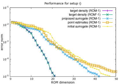
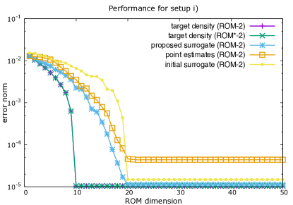
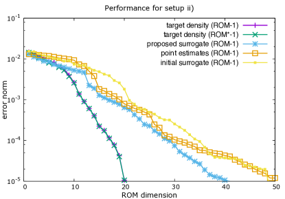
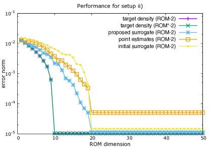
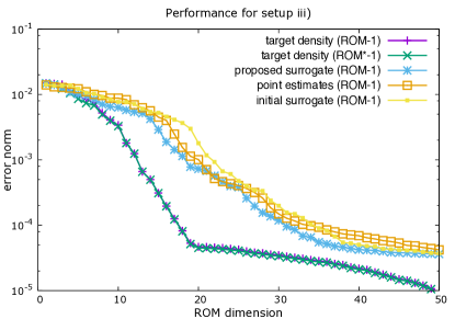
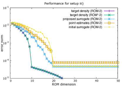
Figure 1: Algorithms performances for construction of ROM-1 and ROM-1^⋆ (on the left) and ROM-2 and ROM-2^⋆ (on the right) for setup $i)$ (above), $ii)$ (middle) and $iii)$ (below). See details in Sections 5.2 and 5.3

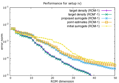
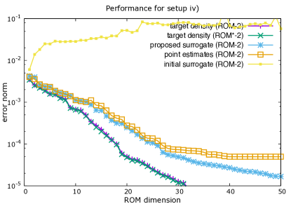
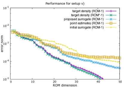
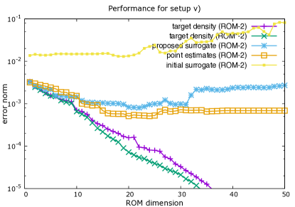
Figure 2: Algorithms performances for construction of ROM-1 and ROM-1^⋆ (on the left) and ROM-2 and ROM-2^⋆ (on the right) for setup $iv)$ (above) and $v)$ (below). See details in Sections 5.2 and 5.3

6 Conclusions

We have proposed a general framework for the construction of ROMs when the distribution of the trajectories of a dynamical system is imperfectly known. This work assumes that we have the following two sources of information at our disposal: 1) an initial surrogate density characterising the trajectories of the system of interest; 2) a set of incomplete observations on the target trajectories obeying a known conditional model.

The ROM construction consists in the minimisation of the expectation of the norm of the error between the true and reduced trajectories. The expectation relies on a data-enhanced surrogate density obtained in a Bayesian setting combining the initial surrogate density and the conditional observation model. We show, that under mild conditions, the proposed data-enhanced surrogate is a better approximation than the initial surrogate in term of the Kullback-Leibler distance to the target density.

We stress the need of approximations to efficiently solve this problem and propose in this context tractable solvers. In particular, we use MC and SMC techniques to characterise our data-enhanced surrogate and propose implementations based on the minimisation of a bound on the objective function. We illustrate how the proposed methodology particularises to two different families of ROMs. We show that these particularisations can be seen as generalisations, in a probabilistic framework, of well-known ROM techniques, namely POD and low-rank DMD. We also show that they can be seen as generalisations of standard ROM constructions based on point estimates.

A numerical evaluation, led in the context of the reduction of a geophysical model, reveals that the proposed methodology may enhance state of the art.

Appendix A Low-Rank Linear Approximation

A.1 Error Bounds

We hereafter show that the error norm for a low-rank linear approximation of (1) can be bounded as presented in Section 4.2. On the one hand, to obtain the lower bound in (30), we notice that according to (41), we have $\tilde{x}_{t}\in\textrm{im}(\mathbf{u}\mathbf{w}_{\mathbf{u}})$ for $t\geq 2$, so that each term contributing to the error norm $\parallel\mathbf{x}-\tilde{\mathbf{x}}(\mathbf{u})\parallel^{2}_{F}=\sum_{t=2}^{T}\|x_{t}-\tilde{x}_{t}(\mathbf{u})\|_{2}^{2}$ can be decomposed into two orthogonal components

$$x_{t}-\tilde{x}_{t}(\mathbf{u})=\underbrace{\mathbf{u}\mathbf{w}_{\mathbf{u}}\mathbf{w}_{\mathbf{u}}^{\intercal}\mathbf{u}^{\dagger}x_{t}-\tilde{x}_{t}(\mathbf{u})}_{\in\,\textrm{im}(\mathbf{u}\mathbf{w}_{\mathbf{u}})}+\underbrace{x_{t}-\mathbf{u}\mathbf{w}_{\mathbf{u}}\mathbf{w}_{\mathbf{u}}^{\intercal}\mathbf{u}^{\dagger}x_{t}}_{\in\,\textrm{im}(\mathbf{u}\mathbf{w}_{\mathbf{u}})^{\perp}}.$$

This implies that

$$\sum_{t=2}^{T}\|x_{t}-\mathbf{u}\mathbf{w}_{\mathbf{u}}\mathbf{w}_{\mathbf{u}}^{\intercal}\mathbf{u}^{\dagger}x_{t}\|^{2}_{2}=\sum_{t=2}^{T}\|x_{t}-\mathbf{u}x_{t-1}\|^{2}_{2}\leq\parallel\mathbf{x}-\tilde{\mathbf{x}}(\mathbf{u})\parallel^{2}_{F}.$$

On the other hand, since elements of the set (28) are such that $\|\mathbf{u}\|_{2,2}\leq\lambda<\infty$, the following result shows the upper bound in (30).

Lemma 1

$\parallel\mathbf{x}-\tilde{\mathbf{x}}(\mathbf{u})\parallel^{2}_{F}\leq c\,\sum_{t=2}^{T}\|x_{t}-\mathbf{u}x_{t-1}\|^{2}_{2},$ with $c=\max_{t\in\{2,...,T\}}\{\sum_{k=t}^{T}(1+4(k-1))\|\mathbf{u}\|_{2,2}^{2(k-t)}\}$.

Proof

Since $\tilde{x}_{t}=\mathbf{u}\tilde{x}_{t-1},$ we have

$$\parallel\mathbf{x}-\tilde{\mathbf{x}}(\mathbf{u})\parallel^{2}_{F} =\sum_{t=2}^{T}\|x_{t}-\mathbf{u}^{t-1}x_{1}\|_{2}^{2}.$$

Using the triangular inequality and the definition of the induced $\ell_{2}$-norm, each term contribution in this sum can be bounded as follows

$$\|x_{t}-\mathbf{u}^{t-1}x_{1}\|_{2} \leq\sum_{\ell=2}^{t}\|\mathbf{u}^{\ell-1}x_{t-\ell+1}-\mathbf{u}^{\ell-2}x_{t-\ell+2}\|_{2},$$

$$\leq\sum_{\ell=2}^{t}\|\mathbf{u}^{\ell-2}\|_{2,2}\|\mathbf{u}x_{t-\ell+1}-x_{t-\ell+2}\|_{2},$$

$$=\sum_{k=2}^{t}\|\mathbf{u}^{t-k}\|_{2,2}\|\mathbf{u}x_{k-1}-x_{k}\|_{2}.$$

Therefore, expanding the square of this sum, we obtain

$$\|x_{t}-\mathbf{u}^{t-1}x_{1}\|^{2}_{2} \leq\sum_{k=2}^{t}\|\mathbf{u}^{t-k}\|^{2}_{2,2}\|\mathbf{u}x_{k-1}-x_{k}\|^{2}_{2}$$

$$+2\sum_{i,j=2|i\neq j}^{t}\|\mathbf{u}^{t-i}\|_{2,2}\|\mathbf{u}x_{i-1}-x_{i}\|_{2}\|\mathbf{u}^{t-j}\|_{2,2}\|\mathbf{u}x_{j-1}-x_{j}\|_{2},$$

$$\leq\sum_{k=2}^{t}\|\mathbf{u}^{t-k}\|^{2}_{2,2}\|\mathbf{u}x_{k-1}-x_{k}\|^{2}_{2}$$

$$+2\sum_{i,j=2|i\neq j}^{t}\max\{\|\mathbf{u}^{t-i}\|^{2}_{2,2}\|\mathbf{u}x_{i-1}-x_{i}\|_{2}^{2},\|\mathbf{u}^{t-j}\|^{2}_{2,2}\|\mathbf{u}x_{j-1}-x_{j}\|_{2}^{2}\},$$

$$\leq\sum_{k=2}^{t}\|\mathbf{u}^{t-k}\|^{2}_{2,2}\|\mathbf{u}x_{k-1}-x_{k}\|^{2}_{2}$$

$$+2\sum_{i,j=2|i\neq j}^{t}\|\mathbf{u}^{t-i}\|^{2}_{2,2}\|\mathbf{u}x_{i-1}-x_{i}\|_{2}^{2}+\|\mathbf{u}^{t-j}\|^{2}_{2,2}\|\mathbf{u}x_{j-1}-x_{j}\|_{2}^{2},$$

$$\leq\sum_{k=2}^{t}(1+4(t-1))\|\mathbf{u}^{t-k}\|^{2}_{2,2}\|\mathbf{u}x_{k-1}-x_{k}\|^{2}_{2}.$$

In consequence, we conclude remarking that

$$\parallel\mathbf{x}-\tilde{\mathbf{x}}(\mathbf{u})\parallel^{2}_{F} \leq\sum_{t=2}^{T}\sum_{k=2}^{t}(1+4(t-1))\|\mathbf{u}^{t-k}\|^{2}_{2,2}\|\mathbf{u}x_{k-1}-x_{k}\|^{2}_{2},$$

$$=\sum_{t=2}^{T}\sum_{k=t}^{T}(1+4(k-1))\|\mathbf{u}^{k-t}\|^{2}_{2,2}\|\mathbf{u}x_{t-1}-x_{t}\|^{2}_{2},$$

$$\leq c\,\parallel\mathbf{x}_{2:T}-\mathbf{u}\mathbf{x}_{1:T-1}\parallel^{2}_{F},$$

with $c=\max_{t\in\{2,...,T\}}\{\sum_{k=t}^{T}(1+4(k-1))\|\mathbf{u}^{k-t}\|^{2}_{2,2}\}$ and where the equality has been obtained by inverting the two sums. $\square$

A.2 Finite Norm of Minimisers

Let $J_{1}(\mathbf{u})=\sum_{t=2}^{T}\|x_{t}-\mathbf{u}x_{t-1}\|^{2}_{2}$, $J_{2}(\mathbf{u})=\|\mathbf{x}-\tilde{\mathbf{x}}(\mathbf{u})\|^{2}_{F}$ and $\mathcal{U}_{k}=\{\mathbf{u}\in\mathds{R}^{n\times n}|\textrm{rank}(\mathbf{u})\leq k\}$.

Lemma 2

Minimisers of $J_{1}$ and $J_{2}$ over the domain $\mathcal{U}_{k}$ have a finite norm.

Proof

First notice that the objective functions are not infinite on all the optimisation domain (e.g., $J_{i}(0)<\infty$ for $i=1,2$). Next, let $\mathcal{U}$ be defined in (28) with $\lambda<\infty$ and

$$\mathcal{U}^{\infty}_{k}=\{\mathbf{u}\in\mathds{R}^{n\times n}|\textrm{rank}(\mathbf{u})\leq k,\|\mathbf{u}\|_{2,2}=\infty\}.$$

We have

$$\operatorname*{arg\,min}_{\mathbf{u}\in\mathcal{U}_{k}}J_{i}(\mathbf{u})\stackrel{{\scriptstyle(a)}}{{=}}\operatorname*{arg\,min}_{\mathbf{u}\in\mathcal{U}\cup\mathcal{U}^{\infty}_{k}}J_{i}(\mathbf{u})\stackrel{{\scriptstyle(b)}}{{=}}\operatorname*{arg\,min}_{\mathbf{u}\in\mathcal{U}\cup(\mathcal{U}_{k^{\prime}}\setminus\mathcal{U}^{\infty}_{k^{\prime}})}J_{i}(\mathbf{u})\stackrel{{\scriptstyle(c)}}{{=}}\operatorname*{arg\,min}_{\mathbf{u}\in\mathcal{U}}J_{i}(\mathbf{u}),\quad\textrm{for }\quad i=1,2,$$

with $k^{\prime}<k$. Equality (a) follows from the decomposition $\mathcal{U}_{k}=\mathcal{U}\cup\mathcal{U}^{\infty}_{k}$. Equality (b) is deduced from the two following facts. For $\mathbf{u}\in\mathcal{U}^{\infty}_{k}$, let $\mathbf{v}^{\infty}_{\mathbf{u}}$ denote the matrix whose columns are the right singular vectors of $\mathbf{u}$ associated to infinite singular values. If $\mathbf{u}$ is such that ${x}_{t-1}\in\textrm{im}(\mathbf{v}^{\infty}_{\mathbf{u}})$ for at least one of the indices $t=2,\cdots,T$ (resp. ${x}_{1}\in\textrm{im}(\mathbf{v}^{\infty}_{\mathbf{u}})$), then $J_{1}(\mathbf{u})=\infty$ (resp. $J_{2}(\mathbf{u})=\infty$) implying that $\mathbf{u}$ is not a minimiser. On the other hand, if $\mathbf{u}$ is such that ${x}_{t-1}\notin\textrm{im}(\mathbf{v}^{\infty}_{\mathbf{u}})$ for any of the indices $t=2,\cdots,T$ (resp. ${x}_{1}\notin\textrm{im}(\mathbf{v}^{\infty}_{\mathbf{u}})$), then there exists $\mathbf{u}^{\prime}\in(\mathcal{U}_{k^{\prime}}\setminus\mathcal{U}^{\infty}_{k^{\prime}})$ such that $J_{1}(\mathbf{u})=J_{1}(\mathbf{u}^{\prime})$ (resp. $J_{2}(\mathbf{u})=J_{2}(\mathbf{u}^{\prime})$). Equality (c) follows from the inclusion $(\mathcal{U}_{k^{\prime}}\setminus\mathcal{U}^{\infty}_{k^{\prime}})\subset\mathcal{U}$. $\square$

Compliance with Ethical Standards

The authors state that there is no conflict of interest.

References

- (1) Agapiou, S., Papaspiliopoulos, O., Sanz-Alonso, D., Stuart, A.M.: Importance Sampling: Computational Complexity and Intrinsic Dimension. ArXiv e-print 1511.06196 (2015)
- (2) Antoulas, A.C.: An overview of approximation methods for large-scale dynamical systems. Annual Reviews in Control 29(2), 181–190 (2005)
- (3) Barrault, M., Maday, Y., Nguyen, N.C., Patera, A.T.: An empirical interpolation method: application to efficient reduced-basis discretization of partial differential equations. Comptes Rendus Mathematique 339(9), 667 – 672 (2004)
- (4) Chandrasekhar, S.: Hydrodynamic and hydromagnetic stability. Courier Corporation (2013)
- (5) Chaturantabut, S., Sorensen, D.C.: Nonlinear model reduction via discrete empirical interpolation. SIAM Journal on Scientific Computing 32(5), 2737–2764 (2010)
- (6) Chen, K.K., Tu, J.H., Rowley, C.W.: Variants of dynamic mode decomposition: boundary condition, koopman, and fourier analyses. Journal of nonlinear science 22(6), 887–915 (2012)
- (7) Ciarlet, P.: The Finite Element Method for Elliptic Problems. Society for Industrial and Applied Mathematics (2002)
- (8) Cohen, A., Devore, R.: Approximation of high-dimensional parametric PDEs. ArXiv e-print 1502.06797 (2015)
- (9) Crisan, D., Doucet, A.: A survey of convergence results on particle filtering methods for practitioners. IEEE Transactions on signal processing 50(3), 736–746 (2002)
- (10) Cui, T., Martin, J., Marzouk, Y.M., Solonen, A., Spantini, A.: Likelihood-informed dimension reduction for nonlinear inverse problems. Inverse Problems 30(11), 114015 (2014)
- (11) Cui, T., Marzouk, Y.M., Willcox, K.E.: Data-driven model reduction for the Bayesian solution of inverse problems. International Journal for Numerical Methods in Engineering 102, 966–990 (2015)
- (12) Doucet, A., Godsill, S., Andrieu, C.: On sequential monte carlo sampling methods for bayesian filtering. Statistics and computing 10(3), 197–208 (2000)
- (13) Everson, R., Sirovich, L.: Karhunen-loève procedure for gappy data. J. Opt. Soc. Am. A 12(8), 1657–1664 (1995)
- (14) Fink, J.P., Rheinboldt, W.C.: On the error behavior of the reduced basis technique for nonlinear finite element approximations. ZAMM - Journal of Applied Mathematics and Mechanics 63(1), 21–28 (1983)
- (15) Gunes, H., Sirisup, S., Karniadakis, G.E.: Gappy data: To krig or not to krig? Journal of Computational Physics 212(1), 358–382 (2006)
- (16) Hasselmann, K.: Pips and pops: The reduction of complex dynamical systems using principal interaction and oscillation patterns. Journal of Geophysical Research: Atmospheres 93(D9), 11,015–11,021 (1988)
- (17) Héas, P., Herzet, C.: Low-rank Approximation and Dynamic Mode Decomposition. ArXiv e-print 1610.02962 (2016)
- (18) Herzet, C., Drémeau, A., Héas, P.: Model Reduction from Partial Observations. ArXiv e-print 1609.08821 (2016)
- (19) Holmes, P., Lumley, J.L., Berkooz, G.: Turbulence, Coherent Structures, Dynamical Systems and Symmetry. Cambridge University Press (1996). Cambridge Books Online
- (20) Jolliffe, I.: Principal Component Analysis. Springer Series in Statistics. Springer (2002)
- (21) Jovanovic, M., Schmid, P., Nichols, J.: Low-rank and sparse dynamic mode decomposition. Center for Turbulence Research Annual Research Briefs pp. 139–152 (2012)
- (22) Kwasniok, F.: The reduction of complex dynamical systems using principal interaction patterns. Phys. D 92(1-2), 28–60 (1996)
- (23) Lorenz, E.N.: Deterministic Nonperiodic Flow. Journal of Atmospheric Sciences 20, 130–148 (1963)
- (24) Maday, Y., Patera, A.T., Penn, J.D., Yano, M.: A parameterized-background data-weak approach to variational data assimilation: formulation, analysis, and application to acoustics. International Journal for Numerical Methods in Engineering 102(5), 933–965 (2015)
- (25) Peherstorfer, B., Willcox, K.: Data-driven operator inference for nonintrusive projection-based model reduction. Computer Methods in Applied Mechanics and Engineering 306, 196–215 (2016)
- (26) Quarteroni, A., Manzoni, A., Negri, F.: Reduced basis methods for partial differential equations: an introduction, vol. 92. Springer (2015)
- (27) Quarteroni, A., Rozza, G., Manzoni, A.: Certified reduced basis approximation for parametrized partial differential equations and applications. Journal of Mathematics in Industry 1(1), 1–49 (2011)
- (28) Sirovich, L.: Turbulence and the dynamics of coherent structures. Quarterly of Applied Mathematics 45, 561–571 (1987)
- (29) Spantini, A., Solonen, A., Cui, T., Martin, J., Tenorio, L., Marzouk, Y.: Optimal low-rank approximations of Bayesian linear inverse problems. ArXiv e-prints (2014)