Incident Light Frequency-based Image Defogging Algorithm

Abstract

Considering the problem of color distortion caused by the defogging algorithm based on dark channel prior, an improved algorithm was proposed to calculate the transmittance of all channels respectively. First, incident light frequency’s effect on the transmittance of various color channels was analyzed according to the Beer-Lambert’s Law, from which a proportion among various channel transmittances was derived; afterwards, images were preprocessed by down-sampling to refine transmittance, and then the original size was restored to enhance the operational efficiency of the algorithm; finally, the transmittance of all color channels was acquired in accordance with the proportion, and then the corresponding transmittance was used for image restoration in each channel. The experimental results show that compared with the existing algorithm, this improved image defogging algorithm could make image colors more natural, solve the problem of slightly higher color saturation caused by the existing algorithm, and shorten the operation time by four to nine times.

Image defog, Dark channel prior, Frequency, Transmittance, Color distortion.

1 Introduction

The images photographed by an imaging device in a foggy environment are born with poor visibility and low contrast, which have direct influence on the safety of aviation, maritime transport and road traffic. Moreover, various outdoor monitoring systems, such as video surveillance system, cannot work reliably in bad weather. Therefore, simple and efficient image defogging is a research subject with an important practical value that can help improve the reliability and robustness of visual systems.

Image defogging technology is an emerging hotspot of research on digital image processing, on which foreign scholars [1, 2, 3, 4, 5, 6, 7] have made extensive studies and achieved a series of theoretical and application results. In summary, image defogging methods fall broadly into two categories [8]: image enhancement-based defogging and physical imaging model-based defogging.

The image enhancement-based defogging method does not consider the cause of image degradation in foggy weather, but merely enhances foggy images in line with their characteristics such as vague detail and low contrast. This can weaken the fog effect on images, improve the visibility of scenes, and enhance the contrast of images. In this image enhancement-based method, that which is the most common is histogram equalization, which can effectively enhance the contrast of images, but owing to the uneven depth of scenes in foggy images, namely different scenes are affected by fog in varying degree, global histogram equalization cannot fully remove the fog effect, while some details are still vague. In Literature [9], the sky is first separated from the rest by local histogram equalization, and then depth information matching is realized skillfully in the non-sky zone by a moving template. This algorithm overcomes the defect of global histogram equalization that processes details ineffectively and avoids the effect of sky noise. But when this algorithm is applied, sub-image selection easily leads to a block effect, and thereby cannot improve the visual effect considerably.

The physical imaging model-based defogging method analyzes and processes the degradation process of foggy images in depth. It first analyzes the inverse generation process of degraded images, and builds a model for atmospheric scattering effect on the attenuation of image contrast in order to restore the definition of degraded images. Generally speaking, since this physical imaging model-based method considers the physical degradation process of foggy images, images can be enhanced more effectively in this way than only image processing is considered. Y. Yitzhaky et al. [10] were the first to consider the cause of foggy image degradation. Based on a detailed analysis of atmospheric effect on image degradation, they built an image degradation model. If atmospheric effect on image degradation is considered to be a process in which images go through a degradation system, an image degradation model can be built to eliminate the influence of weather factors on image quality. However, since the key to building an image degradation model is to determine an atmospheric modulation transfer function, and that the ratio of the effect of atmospheric turbulence and aerosol particles in the atmospheric modulation transfer function has something to do with the meteorological conditions of image photographing, the corresponding local meteorological parameters should be acquired from the meteorological station. However, these parameters are usually hard to get due to the harsh additional conditions.

Recently, He [11]] et al. proposed a simple and effective dark channel prior-based single image defogging method based on the statistical law of outdoor fogless image databases. This method can defog most outdoor images effectively. But in practical application, this algorithm inevitably causes image distortion since excessive color saturation is unavoidable. For this reason, this paper proposed an improved algorithm. First, incident light frequency’s effect on the transmittance of various color channels was analyzed according to the Beer-Lambert’s Law, from which a proportion among various channel transmittances was derived; after that, images were preprocessed by down-sampling to refine transmittance, and then the original size was restored to enhance the operational efficiency of the algorithm; finally, the transmittance of all color channels was acquired in accordance with the proportion, and then the corresponding transmittance was used for image restoration in each channel.

The rest of this paper has the following structure: Section 2 outlines the principle of the defogging algorithm based on dark channel prior; Section 3 analyzes the deficiencies of the original algorithm, and derives an improved algorithm; Section 4 proves the validity of this improved algorithm by comparing it with the existing algorithm in experiments.

2 Dark Channel Prior-based Defogging Algorithm

For a clear description below and an effective comparison in experiments, this section outlines some major dark channel prior-based defogging methods.

2.1 Atmospheric Scattering Model

The atmospheric scattering model proposed by Narasimhan et al. [12, 13, 14, 15, 16] describes the degradation process of foggy images.

$$I(x)=J(x)t(x)+A(1-t(x))$$ (1)

Where $I$ represents the intensity of the image observed, $J$ represents the intensity of scene light, $A$ represents the atmospheric light at infinity, and $t$ is known as transmittance. The first equation item $J(x)t(x)$ is an attenuation term, and $A\left(1-t\left(x\right)\right)$ is an atmospheric light item. The aim of image defogging is to restore $J$ from $I$ .

2.2 Dark Channel Prior

Dark channel prior knowledge comes from statistical observations of a great many outdoor fogless images. It shows that there are always some pixels in the overwhelming majority of images that have a very small value in a color channel. This prior knowledge can be defined as follows:

$$J^{dark}\left(x\right)=\underset{c\in\left\{r,g,b\right\}}{\min}\left(\underset{y\in\Omega\left(x\right)}{\min}\left(J^{c}\left(y\right)\right)\right)$$

$J^{c}$ represents a color channel of $J$ , while $\Omega\left(x\right)$ is a pixel $x$ –centered square area. Suppose $J$ is an outdoor fogless image, and $J^{dark}$ is a dark channel of $J$ , and the above experiential law obtained by observations is known as dark channel prior. Dark channel prior knowledge indicates that the value of $J^{dark}$ is always very low and close to 0.

2.3 Defogging by Dark Channel Prior

Suppose that atmospheric light $A$ has been fixed; then suppose transmittance is constant in a local region. The minimum operator is adopted for Equation (1), and meanwhile $A$ is divided, reducing to:

$$\underset{y\in\Omega\left(x\right)}{\mathop{\min}}\,\left(\frac{{{I}^{c}}\left(y\right)}{{{A}^{c}}}\right)=\tilde{t}\left(x\right)\underset{y\in\Omega\left(x\right)}{\mathop{\min}}\,\left(\frac{{{J}^{c}}\left(y\right)}{{{A}^{c}}}\right)+\left(1-\tilde{t}\left(x\right)\right)$$

Where superscript $c$ denotes the component of a certain color channel, and $\tilde{t}(x)$ denotes a roughly estimated transmittance. The minimum operator is adopted for color channel $c$, so,

$$\underset{c}{\mathop{\min}}\,\left(\underset{y\in\Omega\left(x\right)}{\mathop{\min}}\,\left(\frac{{{I}^{c}}\left(y\right)}{{{A}^{c}}}\right)\right)=\tilde{t}\left(x\right)\underset{c}{\mathop{\min}}\,\left(\underset{y\in\Omega\left(x\right)}{\mathop{\min}}\,\left(\frac{{{J}^{c}}\left(y\right)}{{{A}^{c}}}\right)\right)+\left(1-\tilde{t}\left(x\right)\right)$$ (2)

According to the law of dark channel prior, the dark channel item $J^{dark}$ in the outdoor fogless images should approach 0:

$${{J}^{dark}}\left(x\right)=\underset{c}{\mathop{\min}}\,\left(\underset{y\in\Omega\left(x\right)}{\mathop{\min}}\,\left({{J}^{c}}\left(y\right)\right)\right)=0$$

A rough transmittance can be estimated if the above equation is substituted into (2):

$$\tilde{t}\left(x\right)=1-\underset{c}{\mathop{\min}}\,\left(\underset{y\in\Omega\left(x\right)}{\mathop{\min}}\,\left(\frac{{{I}^{c}}\left(y\right)}{{{A}^{c}}}\right)\right)$$ (3)

It has been discovered in practical application that if fog is removed thoroughly, an image will, however, look unreal, and depth perception will be lost. Therefore, constant $\omega\left(0<\omega\leq 1\right)$ can be introduced to equation (3)to retain some fog:

$$\tilde{t}\left(x\right)=1-\underset{c}{\mathop{\omega\min}}\,\left(\underset{y\in\Omega\left(x\right)}{\mathop{\min}}\,\left(\frac{{{I}^{c}}\left(y\right)}{{{A}^{c}}}\right)\right)$$

Transmittance can only be roughly estimated according to the above equation, so to improve the accuracy, the original paper used an image matting algorithm[17]to refine the transmittance. The following linear equation can be solved to refine the transmittance:

$$\left(L+\lambda U\right)t=\lambda\tilde{t}$$ (4)

where $\lambda$ is a corrected parameter, $L$ is the Laplacian matrix proposed by the image matting algorithm, which is usually a large sparse matrix.

After a refined transmittance $t\left(x\right)$ is obtained, the equation below is used to calculate the resulting image $J\left(x\right)$ of defogging:

$$J\left(x\right)=\frac{I\left(x\right)-A}{\max\left(t\left(x\right),{{t}_{0}}\right)}+A$$ (5)

Where atmospheric light $A$ is estimated this way: sort the pixels in dark channel $J^{dark}$ in descending order in accordance with brightness value, compare the brightness value of the first 0.1% pixels with their brightness value in the original image $I$, and finally take the brightest point as atmospheric light $A$.

For most outdoor foggy images, the above algorithm can achieve a good defogging effect, but color distortion or excessive color saturation may be caused when this algorithm is used to process some images. Moreover, the algorithm runs very slowly. For instance, it will take 38.3 seconds to input an image of 600*455. To solve this problem, this paper improved the original algorithm.

3 Incident Light Frequency-based Algorithm

The imaging formula popular in the machine vision field is adopted in the existing defogging models[16, 13, 15, 12, 14], which was derived based on the Beer-Lambert Law[18]:

$$I(x)={{L}_{\infty}}\rho(x){{e}^{-\beta d(x)}}+{{L}_{\infty}}(1-{{e}^{-\beta d(x)}})$$ (6)

where $I(x)$ represents the brightness value of the pixel at $x$ coordinate in the image, $\rho(x)$ represents the reflection coefficient of various body surfaces, and $e^{-\beta d(x)}$ is transmittance $t$, which represents the attenuation degree of energy when light propagates in atmosphere.

As can be seen from the proof procedure of the Beer-Lambert Law, transmittance is derived from the equation below:

$$t={{e}^{-\int_{{{Z}_{0}}}^{{{Z}_{1}}}{\gamma(\nu,z)dz}}}$$ (7)

where $\nu$ represents incident light frequency, $z$ represents a certain point on the propagation path of incident light. As shown in (7), transmittance $t$ is related to the medium attribute $\gamma\left(\nu,z\right)$ of each point on the propagation path of incident light.

3.1 Original Algorithm Hypotheses

In order to reduce the complexity of the existing defogging model, two hypotheses are made on transmittance $t$ in it.

3.1.1 Suppose incident light has constant frequency

When incident light frequency $\nu$ is constant, equation (7)is simplified into:

$$\begin{split}t&={{e}^{-\int_{{{Z}_{0}}}^{{{Z}_{1}}}{\gamma(\nu,z)dz}}}\\ &={{e}^{-\int_{{{Z}_{0}}}^{{{Z}_{1}}}{\beta*D(z)dz}}}\end{split}$$ (8)

As can be seen in the equation above, the medium attribute function on the propagation path is simplified from bivariate function $\gamma\left(\nu,z\right)$ into single-variable function $D(z)$.

3.1.2 Suppose there are homogeneous atmospheric media on the propagation path of incident light

Under this hypothesis, equation (8) is further simplified into:

$$t ={{e}^{-\int_{{{Z}_{0}}}^{{{Z}_{1}}}{\beta*D(z)dz}}}$$

$$={{e}^{-\beta*\int_{{{Z}_{0}}}^{{{Z}_{1}}}{Ddz}}}$$

$$={{e}^{-\beta d(x)}}$$

Where $d(x)$ represents the field depth at point $x$ in the image, namely the spatial distance between object and imaging device.

3.2 Improvement Direction

Although the above two hypotheses have greatly simplified the complexity of the defogging model, defogging quality have been lowered significantly. In order to further improve defogging quality, we reintroduced the effect of incident light frequency $\nu$ on attenuation coefficient $\beta$ into atmospheric light imaging formula (6), thus further improving the atmospheric light imaging formula, as shown below:

$$I(x)={{L}_{\infty}}\rho(x){{e}^{-\beta(\nu)d(x)}}+{{L}_{\infty}}(1-{{e}^{-\beta(\nu)d(x)}})$$ (9)

At this point, attenuation coefficient $\beta$ is turned into the function $\beta(v)$ of incident light frequency $v$.

According to the distance between object and imaging device (field depth), foggy images can fall into three categories:

• Long-field images. The overwhelming majority of scenes in the images are in the range of long field depth (objects are over 500m away from the camera).

• Short-field images. The overwhelming majority of scenes in the images are in the range of short field depth (objects are less than 500m away from the camera).

• Mixed-field images. Long and short-field scenes exist side by side in the images.

For long-field images, since field depth has increased, the concentration of fog on the propagation path of incident light will show increasingly complex changes with distance increasing. So, the prerequisites for the tenability of Equation (9): media are no longer uniformly distributed on the propagation path of light, and a new atmospheric light model needs to be built. According to the observation of the real world, if an observed object is farther away from the observer, the light from it will be harder to discover and thereby be replaced with atmospheric light (the sum of the various light beams from the environment that interact with each other). Thus, the analytical processing of such images can be translated into that of atmospheric light distribution.

For short-field images, due to the small field depth, the concentration of fog within this range can be considered constant, so such foggy images can be processed by Equation (9).

For mixed-field images, zones can be partitioned according to field depth, and then images can be processed separately in accordance with scene types.

This paper proposed an improved method for the processing of short-field images. As can be seen from Equation (9), the key to the processing of short-field images lies in the calculation of attenuation coefficient $\beta(v)$. That is the focus of research in this paper.

3.3 Attenuation Coefficient

Since only the incident light from such three frequency bands as red (R), Green (G) and Blue (B) is imaged by a sensing method in the current cameras, the analysis of $\beta(v)$ can be limited to R, G and B. A typical frequency value ${{v}_{r}},{{v}_{g}},{{v}_{b}}$ is fetched respectively from R, G and B, which correspond to attenuation coefficient $\beta({{v}_{r}}),\beta({{v}_{g}}),\beta({{v}_{b}})$ respectively. The value of attenuation coefficient can be calculated by the analytical statistics of the attenuation of pure light R, G and B in foggy weather.

After the value of $\beta$(${v}_{r}$),$\beta$(${v}_{g}$),$\beta$(${v}_{b}$) is calculated, their ratio can be computed. The result is denoted by:

$$\beta({{v}_{r}}):\beta({{v}_{g}}):\beta({{v}_{b}})={{\beta}_{r}}:{{\beta}_{g}}:{{\beta}_{b}}$$

The statistical test shows that the effect of image restoration is comparatively ideal when ${{\beta}_{r}}:{{\beta}_{g}}:{{\beta}_{b}}=1:1.28:1.61$.

Suppose it is known that some color channel’s transmittance $t_{c}=e^{-\beta_{c}d(x)}$, other channels’ transmittance $\tilde{t}_{c}={e^{-{{\tilde{\beta}}_{c}}d(x)}}$ can be calculated by it:

$$\begin{split}{{\tilde{t}}_{c}}&={{e}^{-{{\tilde{\beta}}_{c}}d(x)}}\\ &={{e}^{-\lambda{{\beta}_{c}}d(x)}}\\ &={{({{e}^{-{{\beta}_{c}}d(x)}})}^{\lambda}}\\ &={{t}_{c}}^{\lambda}\end{split}$$ (10)

Where $c\in\{r,g,b\},\lambda={{\tilde{\beta}}_{c}}/{{\beta}_{c}}$.

As can be seen in the equation above, once a color channel’s transmittance$t_{c}$ is worked out, other color channels’ transmittance can be calculated according to it, as shown below:

$${{t}_{c}}=\left\{\begin{array}[]{ll}1-\omega\underset{c}{\mathop{\min}}\,\left(\underset{y\in\Omega\left(x\right)}{\mathop{\min}}\,\left(\frac{{{I}^{c}}(y)}{{{A}^{c}}}\right)\right)&;c=d,and\,d~{}is~{}dark~{}channel.\\ {{t}_{d}}^{\lambda}&;c\neq d,then\,\lambda=\frac{{{\beta}_{c}}}{{{\beta}_{d}}}\end{array}\right.$$ (11)

3.4 An Improved Image Restoration Method

Based on the analysis above, this section put forward a new transmittance calculation method.

The main steps are shown as follows:

1. Down-sample output image $I\left(x\right)$, to reduce image size to $\hat{I}\left(x\right)$.

2. Acquire dark channel pixel value ${{\hat{I}}_{d}}\left(x\right)$ and its color channel $d$ according to the formula below:

   $${{\hat{I}}_{d}}\left(x\right)=\underset{c\in\left\{r,g,b\right\}}{\mathop{\min}}\,\left(\underset{y\in\Omega\left(x\right)}{\mathop{\min}}\,\left({{\hat{I}}^{c}}\left(y\right)\right)\right)$$

3. Calculate the transmittance ${{\tilde{t}}_{d}}\left(x\right)$ corresponding to the color channel $d$ in which the dark channel is located using the formula below:

   $${{\tilde{t}}_{d}}\left(x\right)=1-\omega{{\hat{I}}_{d}}\left(x\right)$$ (12)

4. Use image matting algorithm [17] namely solve Equation (4)to refine transmittance ${{\tilde{t}}_{d}}\left(x\right)$ into ${{\hat{t}}_{d}}\left(x\right)$.

5. Restore ${{\hat{t}}_{d}}\left(x\right)$ to the size of the original image by interpolation and get ${{t}_{d}}\left(x\right)$.

6. Calculate the transmittance of all color channels by Equation (11).

7. Restore original image $J\left(x\right)$ in all color channels using the equation below:

   $${{J}_{c}}\left(x\right)=\frac{{{I}_{c}}\left(x\right)-{{A}_{c}}}{\max\left({{t}_{c}}\left(x\right),{{t}_{0}}\right)}+{{A}_{c}}\,\,\,;c\in\{r,g,b\}$$

   The rough operating process of the defogging algorithm is shown in Fig.1.

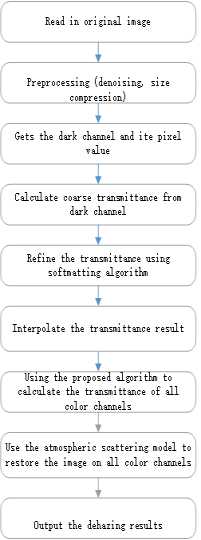
Figure 1: Algorithm processing flow chart.

4 Experiments and Analysis

To test the effect of this algorithm, this paper selected three images: tiananmen of 600*455; house of 441*450; swan of 835*557.

The window $\Omega$ used for dark channel calculation has a size of $5\times 5$, and the $\omega$ in Equation (12) is set equal to 0.95. The algorithm in Literature [17] is still used for image matting.

For the testing experiment in this paper, we adopted the following hardware platform: Intel(R) Core(TM) i3-3220 CPU with a basic frequency of 3.3GHz; 8-G memory with a basic frequency of DDR3 1600MHz. A software platform: MATLAB R2015b 64-bit. All algorithms were implemented through MATLAB code.

Image matting was adopted to refine transmittance in the original algorithm[11]. But this method essentially has high time complexity and space complexity since it is usually used to solve large-scale sparse linear equations. However, the effect of this step on restoration is no more than softening the edge of the transition region between foreground and background to weaken edge effect. Thus, the algorithm proposed in this paper reduces image size significantly, then refines transmittance by image matting, and finally restores the refined transmittance image to the original size by tri-cubic interpolates.

Fig.2 is a comparison of transmittance between the improved algorithm and the original algorithm. As can be seen in the figure, there is little difference between both in edge softening. However, size reduction can help greatly improve the computational efficiency of restoration algorithm. As can be seen in Tab.1, the operating efficiency of the algorithm proposed in this paper is 4~9 times as high as that of the original one.

According to the results before and after improvement shown in Fig.3 to Fig.6, after the transmittance of multiple channels is corrected, the algorithm proposed in this paper solves the problem of slightly higher color saturation in the existing algorithm, and achieves a better and more natural visual effect than the original algorithm.

5 Conclusions

This paper made a theoretical analysis and experimental observation of the dark channel prior-based defogging algorithm, discovering from its theoretical basis that the existing algorithm ignores the effect of incident light frequency on transmittance. Therefore, this paper started with the derivation process of transmittance to reversely derive the relation between various channel transmittances to enhance the defogging algorithm. The experimental results prove that this improved algorithm can achieve a more natural color effect in the restoration result. Since roughly calculated dark channel was still used to compute the relationship between various transmittances, a slight block effect appeared in the restoration result. The current algorithm will be improved at the next step to eradicate this block effect.

(a)

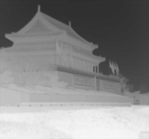
(b)

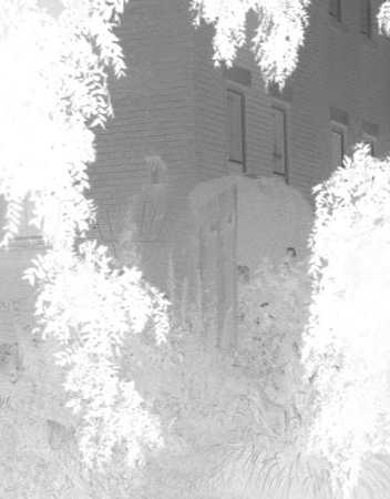
(c)

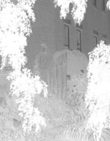
(d)

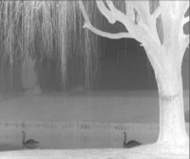
(e)

(f)

Figure 2: Comparison of the transmission maps.

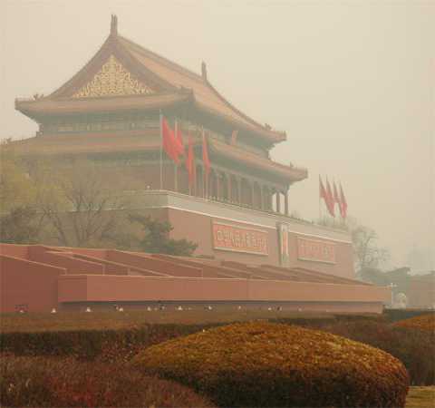
(a) Original

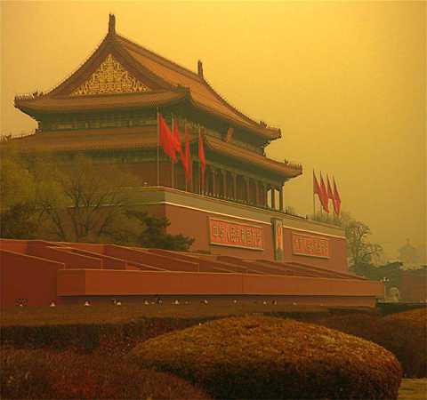
(b) He

(c) This paper

Figure 3: Comparison of the dehazing results.

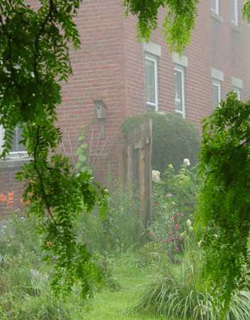
(a) Original

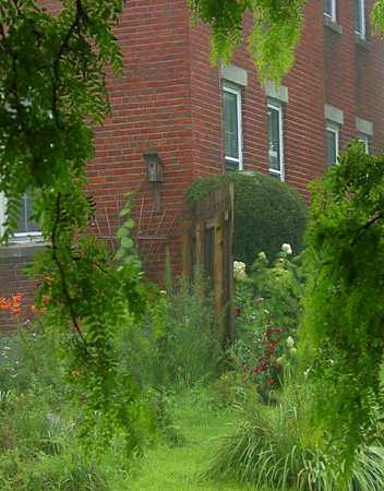
(b) He

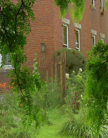
(c) This paper

Figure 4: Comparison of the dehazing results.

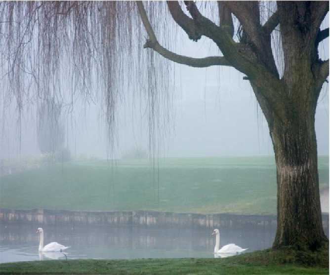
(a) Original

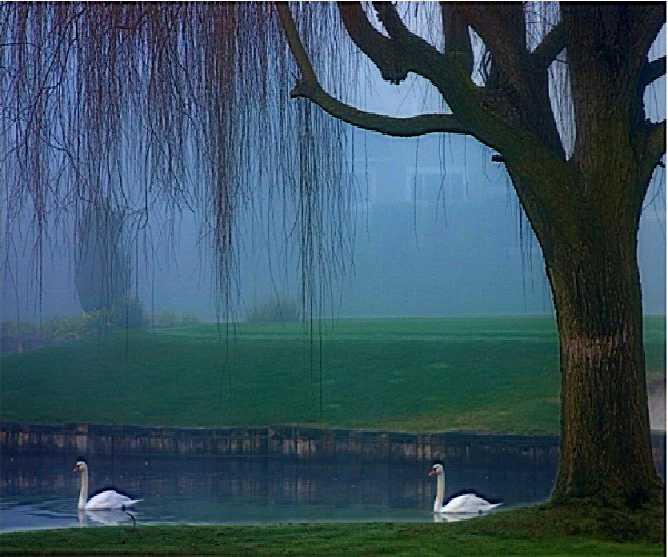
(b) He

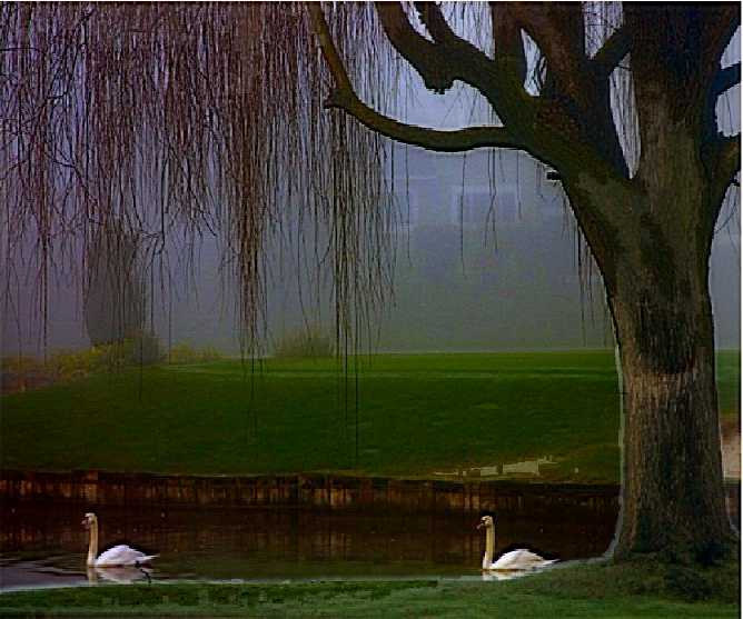
(c) This paper

Figure 5: Comparison of the dehazing results.

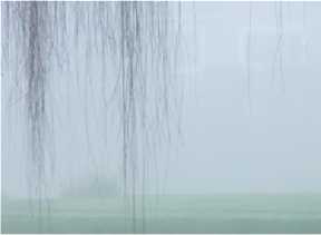
(a) Original

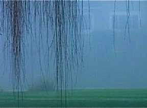
(b) He

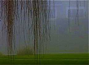
(c) This paper

Figure 6: Comparison of local amplification of the dehazing results.

Image name	Image size	He	This paper	Speed up
tiananmen	600*455	38.30s	5.37s	7.14
house	441*450	27.78s	6.37s	4.36
swan	835*557	70.95s	7.22s	9.82

Table 1: Comparison of time consumption.

References

- [1] L. K. Choi, J. You, and A. C. Bovik, “Referenceless prediction of perceptual fog density and perceptual image defogging,” IEEE Transactions on Image Processing, vol. 24, no. 11, pp. 3888–3901, 2015.
- [2] Q. Zhu, J. Mai, and L. Shao, “A fast single image haze removal algorithm using color attenuation prior,” IEEE Transactions on Image Processing, vol. 24, no. 11, pp. 3522–3533, 2015.
- [3] H. Zhao, C. Xiao, J. Yu, and X. Xu, “Single image fog removal based on local extrema,” IEEE/CAA Journal of Automatica Sinica, vol. 2, no. 2, pp. 158–165, 2015.
- [4] Y.-K. Wang and C.-T. Fan, “Single image defogging by multiscale depth fusion,” IEEE Transactions on Image Processing, vol. 23, no. 11, pp. 4826–4837, 2014.
- [5] Z. Tang, X. Zhang, and S. Zhang, “Robust perceptual image hashing based on ring partition and nmf,” IEEE Transactions on knowledge and data engineering, vol. 26, no. 3, pp. 711–724, 2014.
- [6] Z. Tang, X. Zhang, X. Li, and S. Zhang, “Robust image hashing with ring partition and invariant vector distance,” IEEE Transactions on Information Forensics and Security, vol. 11, no. 1, pp. 200–214, 2016.
- [7] L. Zhang, X. Li, B. Hu, and X. Ren, “Research on fast smog free algorithm on single image,” in 2015 First International Conference on Computational Intelligence Theory, Systems and Applications (CCITSA). IEEE, 2015, pp. 177–182.
- [8] G. Fan, C. Zi-xing, X. Bin, and T. Jin, “Review and prospect of image dehazing techniques [j],” Journal of Computer Applications, vol. 30, no. 9, pp. 2417–2421, 2010.
- [9] Z. Pei, Z. Hong, Q. I. Xue-ming, and L. Han, “An image clearness method for fog,” Jo urnal o f Image and Gra phics, vol. 9, no. 1, pp. 124–128, 2004.
- [10] Y. Yitzhaky, I. Dror, and N. S. Kopeika, “Restoration of atmospherically blurred images according to weather-predicted atmospheric modulation transfer functions,” Optical Engineering, vol. 36, no. 11, pp. 3064–3072, 1997.
- [11] K. He, J. Sun, and X. Tang, “Single image haze removal using dark channel prior,” IEEE transactions on pattern analysis and machine intelligence, vol. 33, no. 12, pp. 2341–2353, 2011.
- [12] S. G. Narasimhan and S. K. Nayar, “Contrast restoration of weather degraded images,” IEEE transactions on pattern analysis and machine intelligence, vol. 25, no. 6, pp. 713–724, 2003.
- [13] ——, “Vision and the atmosphere,” International Journal of Computer Vision, vol. 48, no. 3, pp. 233–254, 2002.
- [14] Y. Y. Schechner, S. G. Narasimhan, and S. K. Nayar, “Instant dehazing of images using polarization,” in Computer Vision and Pattern Recognition, 2001. CVPR 2001. Proceedings of the 2001 IEEE Computer Society Conference on, vol. 1. IEEE, 2001, pp. I–325.
- [15] F. Cozman and E. Krotkov, “Depth from scattering,” in Computer Vision and Pattern Recognition, 1997. Proceedings., 1997 IEEE Computer Society Conference on. IEEE, 1997, pp. 801–806.
- [16] S. K. Nayar and S. G. Narasimhan, “Vision in bad weather,” in Computer Vision, 1999. The Proceedings of the Seventh IEEE International Conference on, vol. 2. IEEE, 1999, pp. 820–827.
- [17] A. Levin, D. Lischinski, and Y. Weiss, “A closed-form solution to natural image matting,” IEEE Transactions on Pattern Analysis and Machine Intelligence, vol. 30, no. 2, pp. 228–242, 2008.
- [18] D. Swinehart, “The beer-lambert law,” J. Chem. Educ, vol. 39, no. 7, p. 333, 1962.