Number-conserving interacting fermion models with exact topological superconducting ground states

Abstract

We present a method to construct number-conserving Hamiltonians whose ground states exactly reproduce an arbitrarily chosen BCS-type mean-field state. Such parent Hamiltonians can be constructed not only for the usual $s$-wave BCS state, but also for more exotic states of this form, including the ground states of Kitaev wires and 2D topological superconductors. This method leads to infinite families of locally-interacting fermion models with exact topological superconducting ground states. After explaining the general technique, we apply this method to construct two specific classes of models. The first one is a one-dimensional double wire lattice model with Majorana-like degenerate ground states. The second one is a two-dimensional $p_{x}+ip_{y}$ superconducting model, where we also obtain analytic expressions for topologically degenerate ground states in the presence of vortices. Our models may provide a deeper conceptual understanding of how Majorana zero modes could emerge in condensed matter systems, as well as inspire novel routes to realize them in experiment.

Introduction.

Topological superconductors have become an active research area in condensed matter and cold atom physics Kitaev ; TPSC-RMP . From a fundamental viewpoint, they provide examples of topological phases that have been classified systematically TPorder1 ; TPorder2 ; TPorder3 ; TPorder4 ; TPorder5 ; TPorder6 . At a practical level, the non-Abelian statistics MR1991 ; Nayak1996 ; Ivanov of Majorana zero modes and the robustness of degenerate ground states against local perturbations have made topological superconductors components of promising architectures for fault-tolerant quantum computation TPQC-RMP . Experimental signatures Exp1 ; Exp2 ; Exp3 ; Exp4 of Majorana zero modes and topological superconductivity in solid state systems call for more realistic theoretical descriptions of the relevant physics, for example the effect of interactions.

Most of the theoretical research in this area has begun with non-interacting mean-field Hamiltonians with an effective $p$-wave pairing term, from which one obtains topologically-protected degenerate ground states and Majorana zero modes that emerge as effective quasiparticles. In nature, however, quantum systems typically contain sizable interacting terms that challenge the validity of mean-field theory. It is therefore important to understand better the criteria for the aforementioned topological phenomena to persist in the interacting case. Moreover, the mean-field approximation breaks the number conservation, which obscures the connection to realistic, number-conserving systems.

Understanding the interplay of topology, number conservation, and interactions is challenging because the interactions usually prevent exact solution by analytic or numerical techniques. In one dimension, special tools are available, and progress has been made using bosonization Bos1 ; Bos2 ; Bos3 and numerical methods [density-matrix renormalization group (DMRG)] PZoller . Exactly solvable models in this area are still rare InteractingKitaev , and the three number-conserving Majorana models RGK ; SDiehl ; NLang that have been proposed are one-dimensional (1D). Having new families of exactly solvable models with realistic local interactions, especially in higher dimensions, will therefore shed light on the characterization of topological phenomena and Majorana zero modes in intrinsically interacting and number-conserving systems. In addition, these results provide new Hamiltonians that can be used to experimentally realize topological states.

In this letter we take a bottom-up approach to these fundamental issues: Starting from a general BCS-type mean-field ground state $\ket{G}$, we show how to construct number-conserving parent Hamiltonians that have $\ket{G}$ as a ground state (with no approximation). This construction enables us to realize the physics of Majorana zero modes in interacting number-conserving systems in an exact manner. Following the general construction, we build specific models including a 1D Majorana double wire and a 2D $p_{x}+ip_{y}$ topological superconductor, and obtain analytic expressions for the degenerate ground states in the presence of edges and vortices.

General construction.

Suppose we have an effective mean-field Hamiltonian in some BCS-like theory in any dimension with or without spin

$$K_{\mathrm{mf}} = \sum_{p}[\xi_{p}a^{\dagger}_{p}a_{p}+\frac{1}{2}(\Delta^{*}_{p}a_{\bar{p}}a_{p}+\Delta_{p}a^{\dagger}_{p}a^{\dagger}_{\bar{p}})]$$ (1)

$$= \sum_{p}E_{p}\alpha_{p}^{\dagger}\alpha_{p}+\mathrm{const},$$

where $E_{p}=\sqrt{\xi_{p}^{2}+|\Delta_{p}|^{2}}$, $p$ indexes the single-particle states (including momentum, spin, or any other quantities necessary), $\bar{p}$ denotes the time reversed state of $p$, and $\alpha_{p}=u_{p}a_{p}-v_{p}a_{\bar{p}}^{\dagger}$ are Bogoliubov quasi-particle operators with $|u_{p}|^{2}+|v_{p}|^{2}=1$ and $v_{p}/u_{p}=-(E_{p}-\xi_{p})/\Delta_{p}^{*}$. The BCS-like ground state of $K_{\text{mf}}$ is (up to normalization)

$$|G\rangle=\sideset{}{{}^{\prime}}{\prod}_{p}\alpha_{p}\alpha_{\bar{p}}|0\rangle,$$ (2)

where the prime means each pair $p\bar{p}$ appears exactly once.

Our goal is to construct a number-conserving Hamiltonian whose ground state is $|G\rangle$. To do this, we first separate each $\alpha_{p}$ into creation and annihilation parts $\alpha_{p}\equiv C_{p}-S_{p}^{\dagger}$ with $C_{p}=u_{p}a_{p}$ and $S_{p}^{\dagger}=v_{p}a_{\bar{p}}^{\dagger}$, and define

$$\hat{A}_{pp^{\prime}}=S^{\dagger}_{p}\alpha_{p^{\prime}}+S^{\dagger}_{p^{\prime}}\alpha_{p}.$$ (3)

From $\alpha_{p}|G\rangle=0$, we know that $\hat{A}_{pp^{\prime}}|G\rangle=0$, and thus a parent Hamiltonian for $|G\rangle$ can be constructed by

$$\hat{H}=\sum_{p_{1}p_{2}p_{3}p_{4}}H_{p_{1}p_{2};p_{3}p_{4}}\hat{A}_{p_{1}p_{2}}^{\dagger}\hat{A}_{p_{3}p_{4}},$$ (4)

where the matrix $H_{p_{1}p_{2};p_{3}p_{4}}$ is required to be Hermitian. This construction suffices for $\ket{G}$ to be a zero-energy eigenstate of $\hat{H}$. To ensure it is a ground state, we require that the matrix $H_{p_{1}p_{2};p_{3}p_{4}}$ is positive-definite. Notice that $\hat{H}$ conserves total particle number ${\hat{N}}=\sum_{p}a_{p}^{\dagger}a_{p}$ since ${\hat{A}}_{pp^{\prime}}$ can be rewritten as

$${\hat{A}}_{pp^{\prime}}=S_{p}^{\dagger}C_{p^{\prime}}+S_{p^{\prime}}^{\dagger}C_{p},$$ (5)

which follows because $S_{p}^{\dagger}S_{p^{\prime}}^{\dagger}+S_{p^{\prime}}^{\dagger}S_{p}^{\dagger}$ vanishes by fermionic antisymmetry. Then the ground state of $\hat{H}$ with a definite particle number $N$ is simply given by the projection of $|G\rangle$ to the $N$-particle subspace $|G_{N}\rangle=\hat{P}_{N}|G\rangle$.

The double wire model.

As a first specific example of this construction, we construct one-dimensional models that reproduce the ground states of Kitaev’s 1D wire Kitaev , $\hat{H}_{\mathrm{Kitaev}}=\sum_{j}(-tc_{j}^{\dagger}c_{j+1}+\Delta c_{j}c_{j+1}+\mathrm{H.c.})-\mu\hat{N}$, where $t$, $\mu$, and $\Delta$ denote the hopping amplitude, the chemical potential and the superconducting gap, respectively. The Kitaev’s model has a special point at $\mu=0,~{}\Delta=t$ where the Hamiltonian can be rewritten as a sum of mutually commuting local operators and the spectrum is non-dispersing Kitaev . To simplify our calculation, we focus on this special point (though our construction protocol is general and could be applied to other points as well Suppl ) where the Hamiltonian has doubly degenerate ground states given by (up to normalization)

$$\ket{G^{e}}=\exp\left(\sum_{i<j}c^{\dagger}_{i}c^{\dagger}_{j}\right)|0\rangle,~{}\ket{G^{o}}=\tilde{c}^{\dagger}_{k=0}|G^{e}\rangle,$$ (6)

where $\tilde{c}^{\dagger}_{k}=\frac{1}{\sqrt{L}}\sum^{L}_{j=1}e^{ikj}c^{\dagger}_{j}$ Suppl . The superscripts $e,o$ denote even and odd fermion parity, respectively.

We consider a double wire geometry that has two parallel one-dimensional chains, with fermion creation operators on each chain given by $a^{\dagger}_{j}\equiv c^{\dagger}_{j,1},~{}b^{\dagger}_{j}\equiv c^{\dagger}_{j,2}$, respectively. Our aim is to construct a number-conserving lattice model on these two wires whose ground states are direct products of the Kitaev ground states on each wire, projected to fixed total particle number $\ket{G_{N}}={\hat{P}}_{N}(\ket{G_{A}}\otimes\ket{G_{B}})$. We will show that the resulting Hamiltonian also leads to Majorana-like edge modes and robust ground state degeneracy.

The direct product of Kitaev ground states $|G_{A}\rangle\otimes|G_{B}\rangle$ is annihilated by Bogoliubov operators Suppl

$$\alpha_{k\sigma} = \frac{e^{i\frac{k}{2}}}{\sqrt{2}}\left(-\sin\frac{k}{2}\tilde{c}_{k\sigma}+i\cos\frac{k}{2}\tilde{c}^{\dagger}_{-k\sigma}\right)-(k\to-k)$$ (7)

$$\equiv C_{k\sigma}-S^{\dagger}_{k\sigma},$$

where $\sigma=1,2$, and the quasimomentum $k$ is quantized with open boundary condition $k=\frac{m\pi}{L},~{}m=1\ldots(L-1)$ .

Having identified the $\alpha_{k\sigma}$, and therefore the $C_{k\sigma}$ and $S_{k\sigma}^{\dagger}$, Eq. (4) gives a family of parent Hamiltonians. By choosing

$$H_{p_{1}p_{2};p_{3}p_{4}}=\frac{16}{L^{2}}\sum_{j=1}^{L}\sin(k_{1}j)\sin(k_{2}j)\sin(k_{3}j)\sin(k_{4}j)$$

$$\times\left[p\delta_{\sigma_{1}\sigma_{2}\sigma_{3}\sigma_{4}}+q\delta_{\sigma_{1}\sigma_{2}}\delta_{\sigma_{3}\sigma_{4}}-r(\delta_{\sigma_{1}\sigma_{3}}\delta_{\sigma_{2}\sigma_{4}}+\delta_{\sigma_{1}\sigma_{4}}\delta_{\sigma_{2}\sigma_{3}})\right],$$ (8)

where $p_{j}=(k_{j},\sigma_{j})$ and $p,q,r$ are arbitrary real coefficients, one obtains Hamiltonians ${\hat{H}}$ with interactions that are local in real space Suppl ,

$$\hat{H} = \sum^{L-1}_{j=1}\left\{-t\left[(a^{\dagger}_{j}a_{j+1}+b^{\dagger}_{j}b_{j+1}+\mathrm{H.c.})-1\right.\right.$$ (9)

$$\left.+2(n^{a}_{j}-\frac{1}{2})(n^{a}_{j+1}-\frac{1}{2})+2(n^{b}_{j}-\frac{1}{2})(n^{b}_{j+1}-\frac{1}{2})\right]$$

$$\left.-(\alpha J^{\dagger}_{||,j}J_{||,j}+\beta J^{\dagger}_{=,j}J_{=,j}+\gamma J^{\dagger}_{\times,j}J_{\times,j})\right\},$$

where $J_{||,j}=b_{j}a_{j}-b_{j+1}a_{j+1},$ $J_{=,j}=a_{j+1}a_{j}-b_{j+1}b_{j},~{}J_{\times,j}=b_{j+1}a_{j}-b_{j}a_{j+1}$ and $\alpha,\beta,\gamma$ are real numbers determined by $p,q,r$ Suppl with constraint $\alpha+\beta+\gamma=0$. In order for the matrix Eq. (8) to be positive-definite, the $\alpha,\beta,\gamma$ should satisfy $\alpha<0,\beta<t,\gamma<t$, which, combined with $\alpha+\beta+\gamma=0$, gives the triangle region that is shown in Fig. 1. The center of the triangle $\alpha=-t,~{}\beta=\gamma=t/2$ reproduces the model in Ref. SDiehl .

Since $\hat{H}$ preserves total particle number $N=N_{A}+N_{B}$ and single wire fermion parity $P^{A,B}=(-1)^{\hat{N}_{A,B}}$, ground states in each $N$-particle sector are doubly degenerate. For example, if $N$ is even, we have (up to normalization)

$$|G_{N}^{ee}\rangle=\left[\sum_{i<j}(a_{i}^{\dagger}a_{j}^{\dagger}+b_{i}^{\dagger}b_{j}^{\dagger})\right]^{\frac{N}{2}}|0\rangle,~{}|G_{N}^{oo}\rangle=\tilde{a}_{0}^{\dagger}\tilde{b}_{0}^{\dagger}|G_{N-2}^{ee}\rangle.$$ (10)

This degeneracy is topologically protected in the sense that all local perturbations in the bulk, even including the ones that violate single wire parity, take the form of an identity matrix when projected to the ground state subspace. For example, using the same arguments as in Refs. NLang ; SDiehl , we explicitly find that the energy splitting $\Delta E$ due to perturbation $a_{j}^{\dagger}b_{j}+\mathrm{H.c.}$ scales as $\Delta E\sim e^{-j/l_{0}}$ (assuming $j<L/2$) for some finite length scale $l_{0}$.

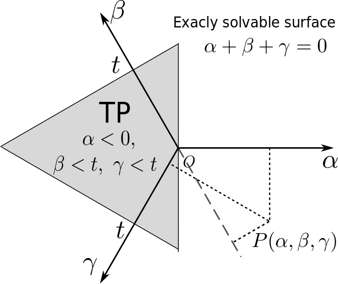
Figure 1: Topological phase (TP) of the double wire system. The constraint $\alpha+\beta+\gamma=0$ restricts the parameter space to the 2D plane drawn in this figure, where the coordinate $(\alpha,\beta,\gamma)$ of an arbitrary point $P$ is given by the projections from $P$ to the $\alpha,\beta,\gamma$ axes. The conditions $\alpha<0,\beta<t,\gamma<t$, which guarantee $\hat{H}$ to be positive definite, give a triangle region (shaded area) in this plane.

The 2D $p_{x}+ip_{y}$ model.

Majorana zero modes are expected to appear at certain boundaries and in the cores of vortices in $p_{x}+ip_{y}$ superconductors. We now show that Eq. (4) can be used to construct number-conserving parent Hamiltonians for $p_{x}+ip_{y}$ topological superconductors that share the same ground state as the mean-field model

$$\hat{K}=\int_{S}\left[\frac{\nabla\psi_{z}^{\dagger}\cdot\nabla\psi_{z}}{2m}-(\Delta\psi_{z}\partial_{\bar{z}}\psi_{z}+\mathrm{H.c.})+\mu\psi_{z}\psi_{z}^{\dagger}\right]d^{2}z,$$ (11)

where $S$ denotes an arbitrary region in the 2D plane with complex coordinates $z=x+iy$, $\partial_{z}=(\partial_{x}-i\partial_{y})/2$, $\partial_{\bar{z}}=(\partial_{x}+i\partial_{y})/2$, $d^{2}z=dxdy$, and $\psi_{z}$ is the fermionic annihilation operator at position $z$. The term $\Delta\psi_{z}\partial_{\bar{z}}\psi_{z}+\mathrm{H.c.}$ characterizes chiral $p$-wave pairing, and $\mu\psi_{z}\psi_{z}^{\dagger}$ is the chemical potential term (which differs from the usual convention by a constant). Although in principle we can construct number-conserving parent Hamiltonians for all values of $(m,\Delta,\mu)$, in the following we only consider a special point $\mu=\frac{m\Delta^{2}}{2}$ and use natural units $2m=m\Delta=1$ for simplicity. With an integration by parts, $\hat{K}$ can be separated into a bulk Hamiltonian and a boundary term $\hat{K}=\hat{K}_{\mathrm{bulk}}+\hat{K}_{\mathrm{bound}}$, with

$$\hat{K}_{\mathrm{bulk}} = \int_{S}(2\partial_{z}\psi_{z}^{\dagger}-\psi_{z})(2\partial_{\bar{z}}\psi_{z}-\psi_{z}^{\dagger})d^{2}z,$$

$$\hat{K}_{\mathrm{bound}} = -i\oint_{\partial S}(\psi_{z}^{\dagger}\partial_{z}\psi_{z}dz+\psi_{z}^{\dagger}\partial_{\bar{z}}\psi_{z}d\bar{z}),$$ (12)

where $\partial S$ denotes the boundary of $S$. Since $\hat{K}_{\mathrm{bulk}}$ is by construction positive-definite, the ground states of $\hat{K}$ should be annihilated by the operator $\alpha_{z}\equiv 2\partial_{\bar{z}}\psi_{z}-\psi_{z}^{\dagger}$ for all $z\in S$ in order to minimize $\hat{K}_{\mathrm{bulk}}$ (we will account for the boundary term momentarily). The ground states with even fermion parity can in general be constructed as

$$|G^{e}\rangle=\exp\left[\frac{1}{2}\int_{S}g(z,z^{\prime})\psi_{z}^{\dagger}\psi_{z^{\prime}}^{\dagger}d^{2}zd^{2}z^{\prime}\right]|0\rangle,$$ (13)

where the two-particle wave function $g(z,z^{\prime})$ satisfies $g(z,z^{\prime})=-g(z^{\prime},z)$ and

$$2\partial_{\bar{z}}g(z,z^{\prime})=\delta^{2}(z-z^{\prime}),$$ (14)

which guarantees that $\alpha_{z}|G^{e}\rangle=0$. To simultaneously minimize the boundary term $\hat{K}_{\mathrm{bound}}$, the function $g(z,z^{\prime})$ should satisfy certain boundary conditions that depend on the geometry of the region $S$, which we will discuss later.

To find a parent Hamiltonian for the mean-field ground state $|G^{e}\rangle$, we again follow our general construction given in Eqs. (4) and (5) where we identify $C_{z}=2\partial_{\bar{z}}\psi_{z}$ and $S^{\dagger}_{z}=\psi^{\dagger}_{z}$, leading to

$$\hat{H}_{\mathrm{bulk}}=\int_{S}W(z_{1},z_{2};z_{3},z_{4})A^{\dagger}_{z_{1},z_{2}}A_{z_{3},z_{4}}\prod^{4}_{j=1}d^{2}z_{j},$$ (15)

where $W(z_{1},z_{2};z_{3},z_{4})$ is a positive-definite Hermitian matrix. We further restrict ourselves to Hamiltonians describing short-ranged interactions, i.e. $W(z_{1},z_{2};z_{3},z_{4})$ tends to zero sufficiently fast when the distance between any two points $|z_{i}-z_{j}|$ becomes large. Furthermore, the boundary term $\hat{K}_{\mathrm{bound}}$ in Eq. (The 2D $p_{x}+ip_{y}$ model.) should be added into $\hat{H}_{\mathrm{bulk}}$ to uniquely pick out the same set of ground states as $\hat{K}$

$$\hat{H}=\hat{H}_{\mathrm{bulk}}+\hat{K}_{\mathrm{bound}}.$$ (16)

The new interacting Hamiltonian $\hat{H}$ harbors the topological $p_{x}+ip_{y}$ ground state. It is number-conserving because both $\hat{H}_{\mathrm{bulk}}$ and $\hat{K}_{\mathrm{bound}}$ preserve total particle number.

As a specific example, we choose $W(z_{1},z_{2};z_{3},z_{4})=w(z_{1}-z_{3})\delta^{2}(z_{1}-z_{2})\delta^{2}(z_{3}-z_{4})/4$ in Eq. (15) where $w(-z)=[w(z)]^{*}$ and $w(0)=1$, after rearranging terms we get

$$\hat{H} = \int_{S}\nabla\psi^{\dagger}_{z}\cdot\nabla\psi_{z}d^{2}z$$

$$+ 4\int_{S}w(z-z^{\prime})\psi^{\dagger}_{z}(\partial_{z^{\prime}}\psi^{\dagger}_{z^{\prime}})\psi_{z^{\prime}}\partial_{\bar{z}}\psi_{z}d^{2}zd^{2}z^{\prime}.$$

The function $w(z-z^{\prime})$ is required to be positive-definite in the matrix sense (i.e. $\tilde{w}_{\mathbf{k}}=\int w(\mathbf{r})e^{i\mathbf{k}\cdot\mathbf{r}}d^{2}\mathbf{r}$ should be real and positive for all $\mathbf{k}$), and should decay sufficiently fast as $|z-z^{\prime}|$ becomes large.

Degenerate ground states with vortices.

It is known that vortices in the mean-field model Eq. (11) have localized Majorana zero-modes NRead ; Ivanov giving rise to topologically-protected degeneracy and non-Abelian statistics. It would be interesting to see whether these important properties survive in our number-conserving model, as these properties are crucial for the realization of topological quantum computation TPQC-RMP . As a first step, we need to obtain the ground state wavefunctions, a calculation whose results we present in this section. One remarkable feature of our model is that the analytic expressions of degenerate ground states could be exactly obtained even when there are an arbitrary number of vortices in the 2D plane. These explicit expressions could give us deeper insight into the topological properties of the ground states and provide a platform to study non-Abelian statistics in number-conserving interacting models in an exact manner.

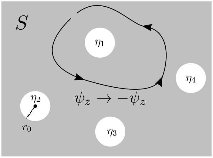
Figure 2: Topological superconducting phase in an unbounded 2D plane with $2M$ vortices located at $\eta_{1},\eta_{2},\ldots,\eta_{2M}$. In this figure we show the $2M=4$ case. In our gauge convention fermion fields acquire a minus sign on going around each vortex.

We consider the geometry shown in Fig. 2, with $2M$ vortices lying in an unbounded 2D plane located at $\eta_{1},\eta_{2},\ldots,\eta_{2M}$, respectively. We assume that the core of each vortex is localized inside a radius $r_{0}$ much smaller than the minimal distance between any two vortices. We use the gauge convention in which the superconducting order parameter is the same everywhere [i.e. still consider the same Hamiltonians in Eqs. (11) and (15)] while fermion fields are anti-periodic around each vortex $\psi^{\dagger}_{\theta+2\pi}=-\psi^{\dagger}_{\theta}$.

In the mean-field model Eq. (11) there is a Majorana zero-mode $\gamma_{j}$ with $\gamma_{j}^{\dagger}=\gamma_{j}$ and $[\gamma_{j},\hat{K}]=0$ localized at the $j^{\mathrm{th}}$ vortex. In total we have $2M$ localized Majorana modes $\gamma_{1},\gamma_{2},\ldots,\gamma_{2M}$ which could be combined to $M$ independent fermion operators $a_{j}=(\gamma_{2j-1}+i\gamma_{2j})/2$, leading to $2^{M}$ degenerate mean-field ground states $|n_{1},n_{2},\ldots,n_{M}\rangle$ with $n_{j}=0,1,~{}1\leq j\leq M$. In our number-conserving model defined in Eq. (16), the ground states with $N$ particles are obtained by projecting the mean-field ground states to the $N$-particles sector. Only those mean-field states with fermion parity equal to $(-1)^{N}$ survive this projection, therefore we are left with $2^{M-1}$ fold degeneracy in each sector.

As an example, we consider the $2M=4$ case and assume $N$ to be even. One of the mean-field ground states $|G_{12,34}\rangle$ could be constructed by Eq. (13) with

$$g_{12,34}(z,z^{\prime}) = \left[\sqrt{\frac{(z-\eta_{1})(z-\eta_{2})(z^{\prime}-\eta_{3})(z^{\prime}-\eta_{4})}{(z^{\prime}-\eta_{1})(z^{\prime}-\eta_{2})(z-\eta_{3})(z-\eta_{4})}}\right.$$ (18)

$$\left.+(z\leftrightarrow z^{\prime})\vphantom{\frac{1}{2}}\right]\frac{1}{4\pi(z-z^{\prime})},$$

where the terms in the bracket is to guarantee that $g_{12,34}(z,z^{\prime})$ is anti-periodic around each vortex, in accordance with our gauge convention. From the identity $2\partial_{\bar{z}}\frac{1}{z-z^{\prime}}=2\pi\delta^{2}(z-z^{\prime})$ it is easy to see that $g_{12,34}(z,z^{\prime})$ satisfies Eq. (14), and it can be checked that the state $|G_{12,34}\rangle$ also minimizes $\hat{K}_{\mathrm{bound}}$ up to some small corrections 2D_TPSC_mf . Applying the projection operator $\hat{P}_{N}$, we get an $N$-particle ground state with multiparticle wave function (up to normalization)

$$\psi_{12,34}(z_{1},z_{2}\ldots z_{N})=\mathrm{Pf}\{g_{12,34}(z_{i},z_{j})\},$$ (19)

where Pf denotes the Pfaffian of the anti-symmetric $N\times N$ matrix $g_{12,34}(z_{i},z_{j})$. The form of the wave function given in Eq. (19) is very similar to one of the Moore-Read Pfaffian states with four quasiholes MR1991 ; Nayak1996 , which were constructed to describe the excitations in the $\nu=5/2$ fractional quantum hall effect (FQHE). By permuting the indices $1,2,3,4$ we get two other degenerate ground states with wave functions $\psi_{13,24}(z_{1}\ldots z_{N})$ and $\psi_{14,23}(z_{1}\ldots z_{N})$. However, using the same method in Ref. Nayak1996 we can prove that these three states are linearly dependent and the space spanned by them is actually two dimensional, consistent with our previous argument.

The non-Abelian statistics of the mean-field ground states of the $p_{x}+ip_{y}$ model have been well-studied in Ref. Ivanov . Braiding the $j^{\mathrm{th}}$ and the $(j+1)^{\mathrm{th}}$ vortices adiabatically gives rise to a unitary rotation $\hat{B}_{jj+1}=\exp(\frac{\pi}{4}\gamma_{j+1}\gamma_{j})$ on the ground state subspace. In our number-conserving model constructed in Eq. (16), the process of braiding preserves total particle number, thus we have to recalculate the Berry’s matrix for each $N$-particle sector, which will be the subject of future work. We expect that such calculation could be done using similar methods in Ref. Bonderson2011 , where unitary evolution of the Moore-Read Pfaffian states due to braiding of quasiholes are calculated with the help of the plasma analogy.

Conclusion.

We have constructed infinite families of number-conserving, interacting Hamiltonians with exact BCS-like ground states, with specific models including a 1D Majorana double wire and a 2D $p_{x}+ip_{y}$ topological superconductor. In the $p_{x}+ip_{y}$ model we obtained analytic expressions of degenerate ground states with four vortices, and pointed out their similarity to the Moore-Read Pfaffian states with four quasiholes constructed in the $\nu=5/2$ FQHE context. Our models give us a deeper theoretical understanding of topological phenomena in interacting systems, set a viable framework for building more realistic models of topological superconductors, and may provide useful guidelines for experimental realization of Majorana zero modes.

I The Double wire model

In this section we first present the detailed derivations of Eqs. (6-9) in the main text, and then we discuss some alternative derivations of the parent Hamiltonian.

I.1 Diagonalization of Kitaev’s Hamiltonian in momentum space with open boundary

To obtain the Bogoliubov operators in Eq. (7) and the form of ground states in Eq. (6) in our main text, here we present the momentum space diagonalization of Kitaev’s Hamiltonian with $\Delta=t$

$$H_{\mathrm{Kitaev}}=\sum_{j}t(-c^{\dagger}_{j}c_{j+1}+c_{j}c_{j+1}+\mathrm{H.c.})-\mu\hat{N}.$$ (S1)

To this end we search for Bogoliubov eigenmodes defined as

$$\alpha_{k}=\sum^{L}_{j=1}(u^{k}_{j}c_{j}+v^{k}_{j}c^{\dagger}_{j}).$$ (S2)

Being the eigenmodes of $H_{\mathrm{Kitaev}}$ with energy $E_{k}>0$, they satisfy $[\alpha_{k},H_{\mathrm{Kitaev}}]=E_{k}\alpha_{k}$, which gives difference equations on $u^{k}_{j},v^{k}_{j}$

$$(E_{k}+\mu)u^{k}_{j} = -t(u^{k}_{j-1}+u^{k}_{j+1})+t(v^{k}_{j-1}-v^{k}_{j+1}),$$

$$(E_{k}-\mu)v^{k}_{j} = t(v^{k}_{j-1}+v^{k}_{j+1})+t(u^{k}_{j+1}-u^{k}_{j-1}),$$ (S3)

with boundary conditions

$$u^{k}_{0}=v^{k}_{0},~{}u^{k}_{L+1}=-v^{k}_{L+1}.$$ (S4)

To solve these equations, we notice that the ansatz solutions

$$u^{k}_{j}=\lambda(k)e^{i(kj-\theta_{k})}-\lambda(-k)e^{-i(kj-\theta_{k})},~{}~{}v^{k}_{j}=e^{i(kj-\theta_{k})}-e^{-i(kj-\theta_{k})}$$ (S5)

with $\lambda(k)=-i\frac{2\Delta\sin k}{E_{k}+\mu+2t\cos k}$ and $E_{k}=\sqrt{\mu^{2}+4t\mu\cos k+4t^{2}}$ satisfy Eq. (I.1). The boundary conditions in Eq. (S4) give constraints on the quasi-momentum $k$ and the real parameter $\theta_{k}$

$$k(L+1)=2\theta_{k}+m\pi,~{}~{}m\in\mathbf{Z},~{}~{}~{}\tan\theta_{k}=\frac{2\Delta\sin k}{E_{k}+\mu+2t\cos k},$$ (S6)

where $0<k<\pi$ and $0<\theta_{k}<\pi/2$. The Bogoliubov operators are (up to normalization)

$$\alpha_{k}=e^{i\theta_{k}}(i\cos\theta_{k}c^{\dagger}_{-k}-\sin\theta_{k}c_{k})-(k\to-k).$$ (S7)

As an aside, we mention that if we replace Eq. (7) in our main text by Eq. (S7) and use the same matrix in Eq. (8), then, still following our general construction, we can get a bigger family of number-conserving, short-range interacting Hamiltonians with ground states $|G^{e,o}\rangle$ depending on $\mu/t$, and this method can be generalized to construct parent Hamiltonians for Kitaev’s ground states at arbitrary points $(t,\Delta,\mu)$ (even including points in the topologically trivial phase).

At the $\mu=0$ point we get especially simple expressions

$$E_{k}=2t,~{}~{}\theta_{k}=\frac{k}{2},~{}~{}k=\frac{m\pi}{L},~{}m=1\ldots(L-1),$$ (S8)

which leads to the single wire version of Bogoliubov operators in Eq. (7) after normalization. To verify that the expressions given in Eq. (6) are indeed the ground states of $H_{\mathrm{Kitaev}}$, we show that $|G^{e}\rangle$ and $|G^{o}\rangle$ are annihilated by all $\alpha_{k}$. We have

$$c_{k}|G^{e}\rangle=\frac{1}{\sqrt{L}}\sum^{L}_{j=1}e^{-ikj}c_{j}~{}\exp\{\sum_{i<j^{\prime}}c^{\dagger}_{i}c^{\dagger}_{j^{\prime}}\}|0\rangle=\frac{1}{\sqrt{L}}\sum_{j,j^{\prime}}e^{-ikj}\mathrm{sgn}(j^{\prime}-j)c^{\dagger}_{j^{\prime}}|G^{e}\rangle=[i\cot\frac{k}{2}c^{\dagger}_{-k}-\frac{1+(-1)^{m}}{1-e^{ik}}c^{\dagger}_{k=0}]|G^{e}\rangle,$$ (S9)

where $\mathrm{sgn}(x)=x/|x|$ for $x\neq 0$ and $\mathrm{sgn}(0)=0$. It follows that

$$[e^{i\frac{k}{2}}\sin\frac{k}{2}c_{k}-(k\to-k)]|G^{e}\rangle=[e^{i\frac{k}{2}}i\cos\frac{k}{2}c^{\dagger}_{-k}-(k\to-k)]|G^{e}\rangle,$$ (S10)

leading to $\alpha_{k}|G^{e}\rangle=0$. Furthermore, it can be easily checked that $\{c^{\dagger}_{k=0},\alpha_{k}\}=0$ for all $k=m\pi/L,~{}1\leq m\leq L-1$, thus $\alpha_{k}|G^{o}\rangle=\alpha_{k}c^{\dagger}_{k=0}|G^{e}\rangle=-c^{\dagger}_{k=0}\alpha_{k}|G^{e}\rangle=0$. We conclude that Eq. (6) indeed gives us the ground states of $H_{\mathrm{Kitaev}}$ at the point $t=\Delta,~{}\mu=0$.

I.2 Detailed derivation of Eq. (9)

To verify that the combination of Eqs. (4) and (8) indeed give the local form of Eq. (9), we first notice that

$$\alpha_{k\sigma} \equiv C_{k\sigma}-S^{\dagger}_{k\sigma}=\frac{e^{i\frac{k}{2}}}{\sqrt{2}}\left(i\cos\frac{k}{2}c^{\dagger}_{-k,\sigma}-\sin\frac{k}{2}c_{k\sigma}\right)-(k\to-k)$$ (S11)

$$= \frac{1}{\sqrt{2L}}\sum^{L-1}_{j=1}\sin kj(c_{j+1,\sigma}+c^{\dagger}_{j+1,\sigma}-c_{j\sigma}+c^{\dagger}_{j\sigma}),~{}~{}k=\frac{m\pi}{L},~{}m=1\ldots(L-1).$$

Using the completeness and orthonormality of $\sin kj$,

$$\sum_{k}\sin kj\sin kj^{\prime}=\frac{L}{2}\delta_{jj^{\prime}},$$ (S12)

we have

$$\frac{4}{\sqrt{2L}}\sum_{k}(C_{k\sigma}-S^{\dagger}_{k\sigma})\sin kj=c_{j+1,\sigma}+c^{\dagger}_{j+1,\sigma}-c_{j\sigma}+c^{\dagger}_{j\sigma}\equiv C_{j\sigma}-S_{j\sigma}^{\dagger},~{}1\leq j\leq L-1,$$ (S13)

where $C_{j\sigma}=c_{j+1,\sigma}-c_{j\sigma},~{}S_{j\sigma}^{\dagger}=-c^{\dagger}_{j+1,\sigma}-c^{\dagger}_{j\sigma}$. The parent Hamiltonian given in Eqs. (4) and (6) can then be expanded in position space (we use the shorthand $\sum_{\boldsymbol{k}}=\sum_{k_{1},k_{2},k_{3},k_{4}}$ and $\sum_{\boldsymbol{\sigma}}=\sum_{\sigma_{1},\sigma_{2},\sigma_{3},\sigma_{4}}$)

$$H = \sum_{p_{1}p_{2}p_{3}p_{4}}H_{p_{1}p_{2};p_{3}p_{4}}\hat{A}^{\dagger}_{p_{1}p_{2}}\hat{A}_{p_{3}p_{4}}=\frac{16}{L^{2}}\sum_{\boldsymbol{k},\boldsymbol{\sigma}}\sum^{L}_{j=1}\sin k_{1}j\sin k_{2}j\sin k_{3}j\sin k_{4}j$$ (S14)

$${}\times\left[p\delta_{\sigma_{1}\sigma_{2}\sigma_{3}\sigma_{4}}+q\delta_{\sigma_{1}\sigma_{2}}\delta_{\sigma_{3}\sigma_{4}}-r(\delta_{\sigma_{1}\sigma_{3}}\delta_{\sigma_{2}\sigma_{4}}+\delta_{\sigma_{1}\sigma_{4}}\delta_{\sigma_{2}\sigma_{3}})\right](C^{\dagger}_{k_{1}\sigma_{1}}S_{k_{2}\sigma_{2}}+C^{\dagger}_{k_{2}\sigma_{2}}S_{k_{1}\sigma_{1}})(S^{\dagger}_{k_{3}\sigma_{3}}C_{k_{4}\sigma_{4}}+S^{\dagger}_{k_{4}\sigma_{4}}C_{k_{3}\sigma_{3}})$$

$$= \frac{64}{L^{2}}\sum_{\boldsymbol{k},\boldsymbol{\sigma}}\sum^{L}_{j=1}(C^{\dagger}_{k_{1}\sigma_{1}}\sin k_{1}j)(S_{k_{2}\sigma_{2}}\sin k_{2}j)(S^{\dagger}_{k_{3}\sigma_{3}}\sin k_{3}j)(C_{k_{4}\sigma_{4}}\sin k_{4}j)$$

$${}\times\left[p\delta_{\sigma_{1}\sigma_{2}\sigma_{3}\sigma_{4}}+q\delta_{\sigma_{1}\sigma_{2}}\delta_{\sigma_{3}\sigma_{4}}-r(\delta_{\sigma_{1}\sigma_{3}}\delta_{\sigma_{2}\sigma_{4}}+\delta_{\sigma_{1}\sigma_{4}}\delta_{\sigma_{2}\sigma_{3}})\right]$$

$$= \sum_{\boldsymbol{\sigma}}\sum^{L}_{j=1}C^{\dagger}_{j\sigma_{1}}S_{j\sigma_{2}}S^{\dagger}_{j\sigma_{3}}C_{j\sigma_{4}}\left[p\delta_{\sigma_{1}\sigma_{2}\sigma_{3}\sigma_{4}}+q\delta_{\sigma_{1}\sigma_{2}}\delta_{\sigma_{3}\sigma_{4}}-r(\delta_{\sigma_{1}\sigma_{3}}\delta_{\sigma_{2}\sigma_{4}}+\delta_{\sigma_{1}\sigma_{4}}\delta_{\sigma_{2}\sigma_{3}})\right]$$

$$= (2t-\beta-\gamma)\sum^{L}_{j=1}[C^{\dagger}_{aj}S_{aj}S^{\dagger}_{aj}C_{aj}+(a\to b)]+(\gamma-\beta)\sum^{L}_{j=1}[C^{\dagger}_{aj}S_{aj}S^{\dagger}_{bj}C_{bj}+(a\leftrightarrow b)]$$

$$+(\beta+\gamma)\sum^{L}_{j=1}(C^{\dagger}_{aj}S_{bj}+C^{\dagger}_{bj}S_{aj})(S^{\dagger}_{aj}C_{bj}+S^{\dagger}_{bj}C_{aj}),$$

where $\beta=-(q+r)/2,~{}\gamma=(q-r)/2$ and $t=(p+q-3r)/2$. By expanding the last line of Eq. (S14) we get the form of Eq. (9) in the main text (with $\alpha=r=-\beta-\gamma$).

I.3 Positive region of $\hat{H}$

We now prove that the matrix $H_{p_{1}p_{2};p_{3}p_{4}}$ given in Eq. (8) is positive semi-definite in the triangle region shown in Fig. 1 in the main text. Notice that $H_{p_{1}p_{2};p_{3}p_{4}}=H_{k_{1}k_{2};k_{3}k_{4}}\cdot\lambda_{\sigma_{1}\sigma_{2};\sigma_{3}\sigma_{4}}$ with orbital part $H_{k_{1}k_{2};k_{3}k_{4}}=\frac{16}{L^{2}}\sum^{L}_{j=1}\sin k_{1}j\sin k_{2}j\sin k_{3}j\sin k_{4}j$ and spin part $\lambda_{\sigma_{1}\sigma_{2};\sigma_{3}\sigma_{4}}=p\delta_{\sigma_{1}\sigma_{2}\sigma_{3}\sigma_{4}}+q\delta_{\sigma_{1}\sigma_{2}}\delta_{\sigma_{3}\sigma_{4}}-r(\delta_{\sigma_{1}\sigma_{3}}\delta_{\sigma_{2}\sigma_{4}}+\delta_{\sigma_{1}\sigma_{4}}\delta_{\sigma_{2}\sigma_{3}})$. The orbital part is always positive, since for any vector $f_{kk^{\prime}}$ we have

$$\sum_{k_{1}k_{2}k_{3}k_{4}}f^{*}_{k_{1}k_{2}}H_{k_{1}k_{2};k_{3}k_{4}}f_{k_{3}k_{4}}=\frac{16}{L^{2}}\sum_{k_{1}k_{2}k_{3}k_{4}}\sum^{L}_{j=1}f^{*}_{k_{1}k_{2}}\sin k_{1}j\sin k_{2}j\sin k_{3}j\sin k_{4}jf_{k_{3}k_{4}}=\frac{16}{L^{2}}\sum^{L}_{j=1}f^{*}_{j}f_{j}\geq 0,$$ (S15)

where $f_{j}=\sum_{kk^{\prime}}f_{kk^{\prime}}\sin kj\sin k^{\prime}j$. For the spin part $\lambda_{\sigma_{1}\sigma_{2};\sigma_{3}\sigma_{4}}$, we write it in the matrix form (assume the order $aa,ab,ba,bb$)

$$\lambda=\begin{bmatrix}p+q-2r&0&0&q\\ 0&-r&-r&0\\ 0&-r&-r&0\\ q&0&0&p+q-2r\end{bmatrix}=\begin{bmatrix}2t-\gamma-\beta&0&0&\gamma-\beta\\ 0&-\alpha&-\alpha&0\\ 0&-\alpha&-\alpha&0\\ \gamma-\beta&0&0&2t-\gamma-\beta\end{bmatrix}=\lambda_{1}\oplus\lambda_{2},$$ (S16)

with $\lambda_{1}=\begin{bmatrix}-\alpha&-\alpha\\ -\alpha&-\alpha\end{bmatrix}$ acting on ($ab,ba$) and $\lambda_{2}=\begin{bmatrix}2t-\gamma-\beta&\gamma-\beta\\ -\gamma-\beta&2t-\gamma-\beta\end{bmatrix}$ acting on $(aa,bb)$. Thus $\lambda$ is positive-definite if and only if both $\lambda_{1}$ and $\lambda_{2}$ are positive-definite. The condition that $\lambda_{1}$ is positive-definite gives $-\alpha>0$, while $\lambda_{2}$ is positive-definite gives $|\gamma-\beta|<2t-\gamma-\beta$, which simplifies to $\alpha<0,~{}\beta<t,~{}\gamma<t$, leading to the triangle region in the main text.

I.4 Alternative derivations of the parent Hamiltonian

The derivation of $\hat{H}$ presented above enables us to see how the double wire model follows from our general construction and can be generalized to arbitrary points of Kitaev’s model. However, for the double wire parent Hamiltonian constructed in our main text, simpler derivations exist. Actually, Eq. (S13) gives us annihilators of the double wire ground state $|G_{A}\rangle\otimes|G_{B}\rangle$ in position space. Thus we can directly build the parent Hamiltonian $\hat{H}$ using the real space version of Eqs. (4) and (5) with $C_{j\sigma}=c_{j+1,\sigma}-c_{j\sigma},~{}S_{j\sigma}^{\dagger}=-c^{\dagger}_{j+1,\sigma}-c^{\dagger}_{j\sigma}$ (or equivalently, directly go to the last line of Eq. (S14) without working in momentum space at all), leading to the same Hamiltonian Eq. (9) in our main text. This derivation is a direct generalization of the one given in Ref. SDiehl .

Another simple derivation is based on using an alternative basis of single wire ground states (at $\Delta=t,\mu=0$) AoP2014

$$|G^{\eta}\rangle = (1+\eta c^{\dagger}_{1})(1+\eta c^{\dagger}_{2})\cdots(1+\eta c^{\dagger}_{L})|0\rangle,~{}~{}\eta=\pm 1,$$ (S17)

and observing the following properties

$$c^{\dagger}_{i}c^{\dagger}_{i+1}|G^{\eta}\rangle = n_{i}n_{i+1}|G^{\eta}\rangle,~{}~{}c_{i+1}c_{i}|G^{\eta}\rangle=\bar{n}_{i}\bar{n}_{i+1}|G^{\eta}\rangle,$$

$$c^{\dagger}_{i}c_{i+1}|G^{\eta}\rangle = n_{i}\bar{n}_{i+1}|G^{\eta}\rangle,~{}~{}c^{\dagger}_{i+1}c_{i}|G^{\eta}\rangle=\bar{n}_{i}n_{i+1}|G^{\eta}\rangle,$$ (S18)

where $\bar{n}_{i}\equiv 1-n_{i}$. With this, it is easy to check that the number-conserving single wire operator $[(c^{\dagger}_{j}c_{j+1}+\mathrm{H.c.})+2(n_{j}-\frac{1}{2})(n_{j+1}-\frac{1}{2})-\frac{1}{2}]$ annihilates $|G^{\eta}\rangle$. To include interwire couplings, we notice that

$$J^{\dagger}_{||,j}J_{||,j}|G^{\eta_{A},\eta_{B}}\rangle=J^{\dagger}_{=,j}J_{=,j}|G^{\eta_{A},\eta_{B}}\rangle=J^{\dagger}_{\times,j}J_{\times,j}|G^{\eta_{A},\eta_{B}}\rangle=(U^{\square}_{j}-U^{(3p)}_{j})|G^{\eta_{A},\eta_{B}}\rangle,$$ (S19)

where $\hat{U}^{\square}_{j}=n^{a}_{j}n^{a}_{j+1}n^{b}_{j}n^{b}_{j+1},~{}~{}\hat{U}^{(3p)}_{j}=[n^{a}_{j}n^{a}_{j+1}(n^{b}_{j}+n^{b}_{j+1})+(a\leftrightarrow b)]$, and $|G^{\eta_{A},\eta_{B}}\rangle=|G^{\eta_{A}}_{A}\rangle\otimes|G^{\eta_{B}}_{B}\rangle$ is the double wire ground state constructed by direct product of single wire ground states. Therefore

$$(\alpha J^{\dagger}_{||,j}J_{||,j}+\beta J^{\dagger}_{=,j}J_{=,j}+\gamma J^{\dagger}_{\times,j}J_{\times,j})|G^{\eta_{A},\eta_{B}}\rangle=0,$$ (S20)

for $\alpha+\beta+\gamma=0$. It then follows that the Hamiltonian constructed in Eq. (9) in the main text satisfies $\hat{H}|G^{\eta_{A},\eta_{B}}\rangle=0$, i.e. $|G^{\eta_{A},\eta_{B}}\rangle$ is an eigenstate of $\hat{H}$ with zero energy. This method can only tell us that $|G^{\eta_{A},\eta_{B}}\rangle$ is an eigenstate of $\hat{H}$. To find the positive region of $\hat{H}$ (where $|G^{\eta_{A},\eta_{B}}\rangle$ become its ground states), we still have to turn to other means.

In Fig. S1 we draw a pictorial representation of the interaction terms of the parent Hamiltonian Eq. (9), including two types of nonlinear terms: interactions and correlated pair tunnelings.

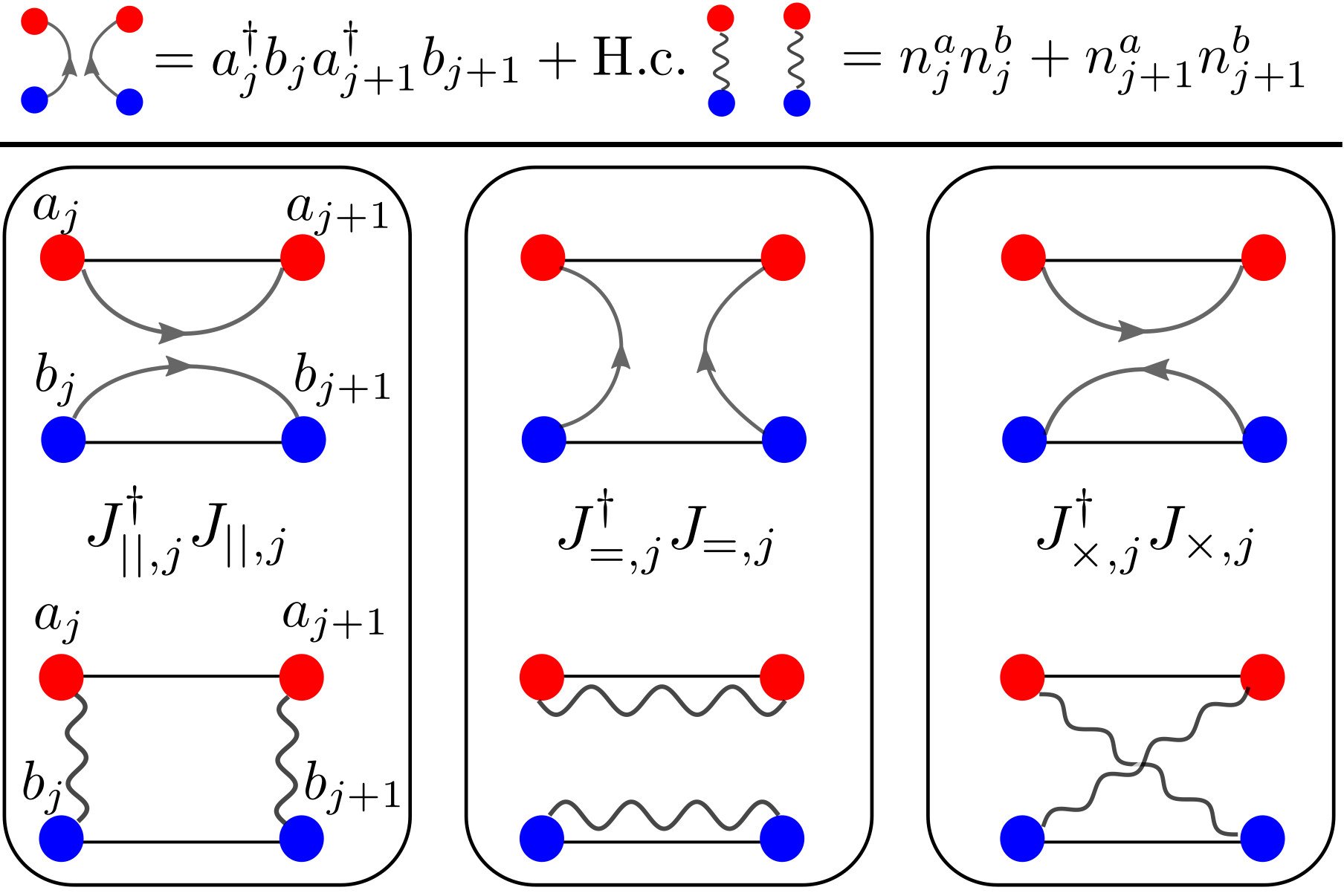
Figure S1: Diagrammatic representation of interaction terms in the double wire parent Hamiltonian in Eq. (9). Double arrows represent pair hopping while wavy lines represent interactions.

References

- (1) M. Greiter, V. Schnells, and R. Thomale, Ann. Phys. 351, 1026 (2014).
- (2) F. Iemini, L. Mazza, D. Rossini, R. Fazio, and S. Diehl, Phys. Rev. Lett. 115, 156402 (2015).