Beamforming and Power Splitting Designs for AN-aided Secure Multi-user MIMO SWIPT Systems

Abstract

In this paper, an energy harvesting scheme for a multi-user multiple-input-multiple-output (MIMO) secrecy channel with artificial noise (AN) transmission is investigated. Joint optimization of the transmit beamforming matrix, the AN covariance matrix, and the power splitting ratio is conducted to minimize the transmit power under the target secrecy rate, the total transmit power, and the harvested energy constraints. The original problem is shown to be non-convex, which is tackled by a two-layer decomposition approach. The inner layer problem is solved through semi-definite relaxation, and the outer problem, on the other hand, is shown to be a single-variable optimization that can be solved by one-dimensional (1-D) line search. To reduce computational complexity, a sequential parametric convex approximation (SPCA) method is proposed to find a near-optimal solution. The work is then extended to the imperfect channel state information case with norm-bounded channel errors. Furthermore, tightness of the relaxation for the proposed schemes are validated by showing that the optimal solution of the relaxed problem is rank-one. Simulation results demonstrate that the proposed SPCA method achieves the same performance as the scheme based on 1-D but with much lower complexity.

I Introduction

In recent years, the idea of energy harvesting (EH) has been introduced to power electronic devices by energy captured from the environment. However, harvesting from natural energy sources such as solar and wind depends on many factors and thus introduces severe reliability issue. Radio frequency (RF) signal can be utilized as an alternative to more reliably deliver energy to EH devices while simultaneously transmitting information [1, 2, 3, 4]. Based on this idea, simultaneous wireless information and power transfer (SWIPT) schemes have been proposed to extend the lifetime of wireless networks [5, 6, 7, 8, 9]. For SWIPT operation in multiple antenna systems [7, 8], co-located receiver architecture employing a power splitter for EH and information decoding (ID) has been studied [9].

On the other hand, in the literature we see increasing research interest in secrecy transmission through physical layer (PHY) security designs [10]. Unlike conventional cryptographic methods which are normally adopted in the network layer and rely on computational security, PHY security approaches are developed from the information-theoretic perspective such that provable secrecy capacity can be achieved [11, 12, 13, 14]. PHY security techniques have been proposed to enhance information security of multiple antenna systems by casting more interference to potential eavesdroppers. By adding artificial noise (AN) and projecting it onto the null space of information user channels in transmit beamforming, the potential eavesdroppers would experience a higher noise floor and thus obtain less information about the messages transmitted to the legitimate receivers [15, 16]. In SWIPT systems, AN injection can improve secrecy capacity of information transmission while not affecting simultaneous power transfer [17, 18, 19, 20, 21, 22, 23, 25, 24]. The AN-aided beamforming for SWIPT operation has been investigated in various multiple-input multiple-output (MIMO) channels [19, 20, 21, 22, 23, 24]. More recently, robust AN-aided transmit beamforming with unknown eavesdroppers was studied for multiple-input single-output (MISO) cognitive radio systems based on different channel uncertainty models [25].

In SWIPT systems, when information receivers (IRs) and energy-harvesting receivers (ERs) are in the same cell, the ERs are normally closer to the transmitter, compared with the IRs, because the power sensitivity level of ER is typically low. This raises a new information security issue for SWIPT systems because the ERs can potentially eavesdrop the information transmission to the IRs with relatively higher received signal strength [20, 23, 26]. In order to guarantee information security for the IRs, it is desirable to implement some mechanism to prevent the ERs from recovering the confidential message from their observations.

Motivated by the aforementioned observations, in this paper, we study secrecy transmission over a multi-user MIMO secrecy channel which consists of one multi-antenna transmitter, multiple legitimate single antenna co-located receivers (CRs) and multiple multi-antenna ERs. We employ an AN injection scheme to mask the desired information-bearing signals for secrecy consideration without imposing any structural restriction on the AN. In comparison with existing works which do not consider power splitter at the legitimate receivers [17, 18, 21, 22], in this paper, each CR is assumed to adopt a power splitter to collect energy from both the information-bearing signal and the AN. The design objective is to jointly optimize the transmit beamforming matrix, the AN covariance matrix, and the power splitting (PS) ratio such that the AN transmit power is maximized subject to constraints on the secrecy rate, the total transmit power, and the energy harvested by both the CRs and the ERs. Because of the coupling effect in the joint optimization problem, determination of the AN covariance matrix and the PS ratio makes the derivation of the secrecy rate and the harvested energy at the CRs more complicated.

The formulated power minimization (PM) problem for AN-aided secrecy transmission is shown to be non-convex, which cannot be solved directly [28]. The PM problem is thus transformed into a two-layer optimization problem and solved accordingly through semi-definite relaxation (SDR) and one-dimensional (1D) line search. We first propose a joint optimization design for the case with perfect channel state information (CSI). The framework is then extended to robust designs for systems having deterministic or statistical CSI uncertainties. The contributions of this work are summarized as follows:

• For the case with perfect CSI at the transmitter, the inner loop of the PM problem is solved through SDR, while the outer loop is shown to be a single-variable optimization problem, where a one-dimensional line search algorithm is employed to find the optima. To reduce computational complexity, a sequential parametric convex approximation (SPCA) method is also investigated [14, 24, 32].

• For the imperfect CSI case with deterministic channel uncertainties, we consider a worst-case robust PM (WCR-PM) problem. By exploiting the S-procedure [28], the semi-infinite constraints are transformed into linear matrix inequalities (LMIs) and the inner loop can be relaxed into an SDP by employing the SDR method. The corresponding robust optimal design is proposed. Furthermore, an SPCA-based iterative algorithm is also addressed with low complexity.

• For both the perfect CSI and imperfect CSI cases, the tightness of the SDP relaxation is verified by showing that the optimal solution is rank-one.

Compared with our preliminary work [23], major additional work and results incorporated in this paper are summarized in the following. 1) This paper has extended the problem of AN power maximization to both perfect and imperfect CSI cases, which introduces substantial changes in the analyses. 2) An SPCA-based iterative algorithm has been proposed to solve the problem such that the computational complexity is largely reduced compared with the 1-D search method used in the previous work.

The rest of this paper is organized as follows: The system model of a multi-user MIMO secrecy channel with SWIPT is presented in Section II. Section III investigates the transmit beamforming based PM problem with perfect CSI. Section IV extends the PM results to the imperfect CSI case. Section V illustrates the computational complexity of the proposed algorithms. The numerical results are shown in Section VI. Finally, we conclude the paper in Section VII.

Notation: Vectors and matrices are denoted by bold lowercase and bold uppercase letters, respectively. $(\cdot)^{T}$ and $(\cdot)^{H}$ represent matrix transpose and Hermitian transpose. The operator $\otimes$ represents the Kronecker product. For a vector x, $\|\textbf{\emph{x}}\|$ indicates the Euclidean norm. $\mathbb{C}^{M\times L}$ and $\mathbb{H}^{M\times L}$ denote the space of ${M\times L}$ complex matrices and Hermitian matrices, respectively. $\mathbb{H}_{+}$ represents the set of positive semi-definite Hermitian matrices, and $\mathbb{R}_{+}$ denotes the set of all nonnegative real numbers. For a matrix A, ${\textbf{A}}\succeq\textbf{0}$ means that A is positive semi-definite, and $\|\textbf{{A}}\|_{F}$, $\rm{tr}({\textbf{A}})$, $|{\textbf{A}}|$ and $\rm{rank}({\textbf{A}})$ denote the Frobenius norm, trace, determinant, and the rank, respectively. ${{\emph{vec}}}(\textbf{{A}})$ stacks the elements of A in a column vector. $\mathbf{0}_{M\times L}$ is a zero matrix of size ${M\times L}$. $\mathrm{E}\{\cdot\}$ is the expectation operator, and $\Re\{\cdot\}$ stands for the real part of a complex number. $[x]^{+}$ represents $\max\{x,0\}$ and $\lambda_{max}(\textbf{{A}})$ denotes the maximum eigenvalue of A.

II System Model

In this section, we consider a multi-user MIMO secrecy channel which consists of one multi-antenna transmitter, $L$ single-antenna CRs and $K$ multi-antenna ERs. We assume that each CR employs the PS scheme to receive the information and harvest power simultaneously. It is assumed that the transmitter is equipped with $N_{T}$ transmit antennas, and each ER has $N_{R}$ receive antennas.

We denote by $\mathbf{h}_{c,l}\in\mathbb{C}^{N_{T}}$ the channel vector between the transmitter and the $l$-th CR, and $\mathbf{H}_{e,k}\in\mathbb{C}^{N_{T}\times N_{R}}$ the channel matrix between the transmitter and the $k$-th ER. The received signal at the $l$-th CR and the $k$-th ER are given by

$$\begin{split}y_{c,l}&=\mathbf{h}_{c,l}^{H}\mathbf{x}\!+\!n_{c,l},~{}\forall l,\\ \mathbf{y}_{e,k}&=\mathbf{H}_{e,k}^{H}\mathbf{x}\!+\!\mathbf{n}_{e,k},~{}\forall k,\end{split}$$

where $\mathbf{x}\in\mathbb{C}^{N_{T}}$ is the transmitted signal vector, and $n_{c,l}\sim\mathcal{CN}(0,\sigma_{c,l}^{2})$ and $\mathbf{n}_{e,k}\sim\mathcal{CN}(0,\sigma_{k}^{2}\mathbf{I})$ are the additive Gaussian noise at the $l$-th CR and the $k$-th ER, respectively.

In order to achieve secure transmission, the transmitter employs transmit beamforming with AN, which acts as interference to the ERs, and provides energy to the CRs and ERs. The transmit signal vector $\mathbf{x}$ can be written as

$$\mathbf{x}=\mathbf{q}s+\mathbf{w},$$ (1)

where $\mathbf{q}\in\mathbb{C}^{N_{T}}$ defines the transmit beamforming vector, $s$ with $\mathrm{E}\{s^{2}\}=1$ is the information-bearing signal intended for the CRs, and $\mathbf{w}\in\mathbb{C}^{N_{T}}$ represents the energy-carrying AN, which can also be composed by multiple energy beams.

As the CR adopts PS to perform ID and EH simultaneously, the received signal at the $l$-th CR is divided into ID and EH components by the PS ratio $\rho_{c,l}\in(0,1]$. Therefore, the signal for information detection at the $l$-th CR is given by

$$y_{c,l}^{ID}=\sqrt{\rho_{c,l}}y_{c,l}\!+\!n_{p,l}=\sqrt{\rho_{c,l}}(\mathbf{h}_{c,l}^{H}\mathbf{x}\!+\!n_{c,l})\!+\!n_{p,l},~{}\forall l,$$

where $n_{p,l}\sim\mathcal{CN}(0,\sigma_{p,l}^{2})$ is the additive Gaussian noise at the $l$-th CR.

Denoting $\mathbf{Q}=\mathrm{E}\{\mathbf{q}\mathbf{q}^{H}\}$ as the transmit covariance matrix and $\mathbf{W}=\mathrm{E}\{\mathbf{w}\mathbf{w}^{H}\}$ as the AN covariance matrix, the achieved secrecy rate at the $l$-th CR is given by

$$\begin{split}\hat{R}_{c,l}&=\bigg{[}\log\bigg{(}1\!+\!\frac{\rho_{c,l}\mathbf{h}_{c,l}^{H}\mathbf{Q}\mathbf{h}_{c,l}}{\rho_{c,l}(\sigma_{c,l}^{2}\!+\!\mathbf{h}_{c,l}^{H}\mathbf{W}\mathbf{h}_{c,l})\!+\!\sigma_{p,l}^{2}}\bigg{)}\\ &-\max_{k}\log\bigg{|}\mathbf{I}\!+\!(\mathbf{H}_{e,k}^{H}\mathbf{W}\mathbf{H}_{e,k}\!+\!\sigma_{k}^{2}\mathbf{I})^{-1}\mathbf{H}_{e,k}^{H}\mathbf{Q}\mathbf{H}_{e,k}\bigg{|}\bigg{]}^{+},~{}\forall l.\end{split}$$ (2)

The harvested power at the $l$-th CR and the $k$-th ER is therefore

$$\begin{split}E_{c,l}&=\eta_{c,l}(1\!-\!\rho_{c,l})\big{(}\mathbf{h}_{c,l}^{H}(\mathbf{Q}\!+\!\mathbf{W})\mathbf{h}_{c,l}\!+\!\sigma_{c,l}^{2}\big{)},~{}\forall l,\\ E_{e,k}&=\eta_{e,k}\bigg{(}\textrm{tr}\big{(}\mathbf{H}_{e,k}^{H}(\mathbf{Q}\!+\!\mathbf{W})\mathbf{H}_{e,k}\big{)}\!+\!N_{R}\sigma_{k}^{2}\bigg{)},~{}\forall k,\end{split}$$ (3)

where $\eta_{c,l}$ and $\eta_{e,k}$ represent the EH efficiency of the $l$-th CR and the EH efficiency of the $k$-th ER, respectively. In this paper we set $\eta_{c,l}=\eta_{e,k}=0.3$ for simplicity. The results can be easily extended to scenarios with different $\eta_{c,l}$ and $\eta_{e,k}$ values. In the following section, we consider the transmit beamforming based PM problem to jointly optimize the transmit covariance matrix $\mathbf{Q}$, the AN covariance matrix $\mathbf{W}$, and the PS ratio $\rho_{c,l}$.

III Masked Beamforming Based Power Minimization with Perfect CSI

In this section, we study transmit beamforming optimization under the assumption that perfect CSI of all the channels is available at the transmitter.

III-A Problem Formulation

In this problem, the transmit power of the information signal is minimized subject to the total transmit power constraint, the secrecy rate constraint, and the EH constraints of the CRs and the ERs such that the AN transmit power is maximized for secrecy consideration. The AN-aided PM problem is thus formulated as

$$\min_{\mathbf{Q},{\kern 1.0pt}\mathbf{W},{\kern 1.0pt}\rho_{c,l}} ~{}~{}~{}~{}~{}~{}~{}~{}~{}~{}~{}~{}\textrm{tr}(\mathbf{Q})$$

s.t. $$\!\!\!\!\!\!\!\!\!\!\!\!\!\!\log\bigg{(}1\!+\!\frac{\rho_{c,l}\mathbf{h}_{c,l}^{H}\mathbf{Q}\mathbf{h}_{c,l}}{\rho_{c,l}(\sigma_{c,l}^{2}\!+\!\mathbf{h}_{c,l}^{H}\mathbf{W}\mathbf{h}_{c,l})\!+\!\sigma_{p,l}^{2}}\bigg{)}$$ (4e)

$$\!\!\!\!\!\!\!\!\!\!\!\!\!\!\!\!\!\!\!\!\!\!\!\!\!\!\!\!\!\!\!\!\!\!\!\!\!\!\!\!\!\!\!-\max_{k}\log\bigg{|}\mathbf{I}+(\sigma_{k}^{2}\mathbf{I}\!+\!\mathbf{H}_{e,k}^{H}\mathbf{W}\mathbf{H}_{e,k})^{-1}\mathbf{H}_{e,k}^{H}\mathbf{Q}\mathbf{H}_{e,k}\bigg{|}\!\geq\!\bar{R}_{c,l},$$

$$\!\!\!\!\!\!\!\!\!\!\!\!\!\!\!\!\!\!\!\!\!\!\!\textrm{tr}(\mathbf{Q}+\mathbf{W})\leq P,$$

$$\!\!\!\!\!\!\!\!\!\!\!\!\!\!\!\!\!\!\!\!\!\!\!\mathbf{h}_{c,l}^{H}(\mathbf{Q}+\mathbf{W})\mathbf{h}_{c,l}+\sigma_{c,l}^{2}\geq\frac{\bar{E}_{c,l}}{\eta_{c,l}(1-\rho_{c,l})},$$

$$\!\!\!\!\!\!\!\!\!\!\!\!\!\!\!\!\!\!\!\!\!\!\!\min_{k}\textrm{tr}\big{(}\mathbf{H}_{e,k}^{H}(\mathbf{Q}\!+\!\mathbf{W})\mathbf{H}_{e,k}\big{)}\!+\!N_{R}\sigma_{k}^{2}\geq\frac{\bar{E}_{e,k}}{\eta_{e,k}},\forall k,$$

$$\!\!\!\!\!\!\!\!\!\!\!\!\!\!\!\!\!\!\!\!\!\!\!\mathbf{Q}\succeq\mathbf{0},\mathbf{W}\succeq\mathbf{0},0<\rho_{c,l}\leq 1,\forall l,\textrm{rank}(\mathbf{Q})\!=\!1,$$

where $\bar{R}_{c,l}$ is the target secrecy rate, $P$ is the total transmit power, and $\bar{E}_{c,l}$ and $\bar{E}_{e,k}$ denote the predefined harvested power at the $l$-th CR and the $k$-th ER, respectively. The constraint (4e) guarantees that a minimum energy harvested power should be achieved by the $k$-th ER.

III-B One-Dimensional Line Search Method (1-D Search)

Problem (4) is non-convex due to the secrecy rate constraint (4e), and thus cannot be solved directly. In order to circumvent this issue, we convert the original problem by introducing a slack variable $t$ for the $k$-th ER’s rate. Then we have

$$\!\!\!\!\!\!\!\!\!\!\!\!\!\!\!\min_{\mathbf{Q},{\kern 1.0pt}\mathbf{W},{\kern 1.0pt}\rho_{c,l},{\kern 1.0pt}t}~{}~{}~{}~{}~{}~{}\textrm{tr}(\mathbf{Q})$$

$$\!\!\!\!\!\!\!\!\!\!\!\!\!\!\!\mbox{s.t.}~{}~{}\!\log\bigg{(}t\!+\!\frac{t\rho_{c,l}\mathbf{h}_{c,l}^{H}\mathbf{Q}\mathbf{h}_{c,l}}{\rho_{c,l}(\sigma_{c,l}^{2}\!+\!\mathbf{h}_{c,l}^{H}\mathbf{W}\mathbf{h}_{c,l})\!+\!\sigma_{p,l}^{2}}\bigg{)}\!\geq\!\bar{R}_{c,l},\forall l,$$ (5a)

$$\!\!\!\!\!\!\!\bigg{|}\mathbf{I}\!+\!(\sigma_{k}^{2}\mathbf{I}\!+\!\mathbf{H}_{e,k}^{H}\mathbf{W}\mathbf{H}_{e,k})^{-1}\mathbf{H}_{e,k}^{H}\mathbf{Q}\mathbf{H}_{e,k}\bigg{|}\!\leq\!\frac{1}{t},\forall k,$$ (5b)

$$\!\!\!\!\!\!\!\eqref{eq:Power_constraints}-\eqref{eq:Another_constraints_ori}.$$

Problem (5) is still non-convex in constraints (5a) and (5b), which can be addressed by reformulating (5) into a two-layer problem. For the inner layer, we solve problem (5) for a given $t$, which is relaxed as

$$\!\!\!\!\!\!\!\!\!\!\!\!\!\!\!\!\!\!\!\!\!\!f(t)=\min_{\mathbf{Q},{\kern 1.0pt}\mathbf{W},{\kern 1.0pt}\rho_{c,l},{\kern 1.0pt}t}~{}~{}\textrm{tr}(\mathbf{Q})$$

$$\!\!\!\!\!\!\!\!\!\!\!\!\!\!\!\!\!\!\!\!\!\!\mbox{s.t.}~{}\mathbf{h}_{c,l}^{H}\big{(}t\mathbf{Q}\!-\!(2^{\bar{R}_{c,l}}\!-\!t)\mathbf{W}\big{)}\mathbf{h}_{c,l}\!\geq\!(2^{\bar{R}_{c,l}}\!-\!t)\big{(}\sigma_{c,l}^{2}\!+\!\frac{\sigma_{p,l}^{2}}{\rho_{c,l}}\big{)},$$ (6a)

$$\!\!\!\!({\textstyle{1\over t}}\!-\!1)(\sigma_{k}^{2}\mathbf{I}\!+\!\mathbf{H}_{e,k}^{H}\mathbf{W}\mathbf{H}_{e,k})\!\succeq\!\mathbf{H}_{e,k}^{H}\mathbf{Q}\mathbf{H}_{e,k},\forall k,$$ (6b)

$$\!\!\!\!\eqref{eq:Power_constraints}-\eqref{eq:Another_constraints_ori},$$

where $f(t)$ is defined as the optimal value of problem (6), which is a function of $t$. Even though the function $f(t)$ cannot be expressed in closed-form, numerical evaluation of $f(t)$ is feasible.

Remark 1: It is noted that the LMI constraint (6b) is obtained from [16, Proposition 1], and is based on the assumption that $\textrm{rank}(\mathbf{Q})\leq 1$, which will be shown later.

By ignoring the non-convex constraint $\textrm{rank}(\mathbf{Q})=1$, problem (6) becomes convex and thus can be solved efficiently by an interior-point method for any given $t$ [28]. The outer layer problem, whose objective is to find the optimal value of $t$, is then formulated as

$$\begin{split}&\min_{t}~{}f(t)\\ &\mbox{s.t.}~{}~{}t_{\textrm{min}}\!\leq\!t\!\leq\!t_{\textrm{max}},\end{split}$$ (7)

where $t_{\textrm{max}}$ and $t_{\textrm{min}}$ are the upper and lower bounds of $t$, respectively. The solution to problem (7) can be found by one-dimensional line search. For the line search algorithm, we need to determine the lower and upper bounds of the searching interval for $t$. It is straightforward that $t_{\textrm{max}}=1$ can be used as the upper bound due to the feasibility of (5b), while a lower bound is calculated as

$$t \geq\min_{l}\bigg{(}1+\frac{\rho_{c,l}\mathbf{h}_{c,l}^{H}\mathbf{Q}\mathbf{h}_{c,l}}{\rho_{c,l}(\sigma_{c,l}^{2}+\mathbf{h}_{c,l}^{H}\mathbf{W}\mathbf{h}_{c,l})+\sigma_{p,l}^{2}}\bigg{)}^{-1}$$

$$\geq\min_{l}\bigg{(}1+\frac{\mathbf{h}_{c,l}^{H}\mathbf{Q}\mathbf{h}_{c,l}}{\sigma_{c,l}^{2}+\sigma_{p,l}^{2}+\mathbf{h}_{c,l}^{H}\mathbf{W}\mathbf{h}_{c,l}}\bigg{)}^{-1}$$

$$\geq\min_{l}\bigg{(}1+\frac{P\|\mathbf{h}_{c,l}\|^{2}}{\sigma_{c,l}^{2}+\sigma_{p,l}^{2}}\bigg{)}^{-1}\triangleq t_{\textrm{min}}.$$

where the first inequality is based on the secrecy rate $\bar{R}_{c,l}\geq 0$, the third inequality follows from (4e). In the following theorem, we prove the equivalence of problem (7) and the original problem (4).

Theorem 1: The transmit beamforming PM problem (4) is equivalent to problem (7) when $\textrm{rank}(\mathbf{Q})\leq 1$.

Proof: Let us denote the optimal solutions of (4) and (7) as $f^{*}$ and $f^{\rm{opt}}$, respectively. First, we show that $f^{\rm{opt}}$ is a feasible point of problem (7), i.e. $f^{\rm{opt}}\leq f^{*}$. It is noted that (4) and (6) have the same objective function and the optimal solution of (4) satisfies the constraints of (6) given the assumption that $\textrm{rank}(\mathbf{Q})\leq 1$ [16], which gives rise to $f(t^{*})=f^{*}$, where $t^{*}$ is the optimal value of $t$. In addition, it follows $f^{\rm{opt}}\leq f(t^{*})$. Next, we prove that the solution to problem (6) is achievable in problem (4), i.e. $f^{*}\leq f^{\rm{opt}}$. From (4e), (6a) and (6b), we can show that the optimal solutions of (6) are feasible solutions of (4e) when $\textrm{rank}(\mathbf{Q})\leq 1$. Therefore, we conclude that $f^{*}=f^{\rm{opt}}$.                                                           $\blacksquare$

Utilizing the results in Remark 1 and Theorem 1, next we show the tightness of the AN-aided PM problem (4) by the following theorem.

Theorem 2: Provided that problem (6) is feasible for a given $t>0$, there exists an optimal solution to (4) such that the rank of $\mathbf{Q}$ is always equal to 1.

Proof: See Appendix A.                                                        $\blacksquare$

Problem (7) can be solved by conducting one-dimensional line search for $f(t)$ over $t$ and choosing the minimum $f(t)$ as the optimal solution. Solving the SDP problem (6) with the optimal $f(t)$, we can obtain the optimal design variables $(\mathbf{Q}^{*},{\kern 1.0pt}\mathbf{W}^{*},{\kern 1.0pt}\rho_{c,l}^{*})$. The optimal beamforming vector $\mathbf{q}^{*}$ is then computed by eigenvalue decomposition $\mathbf{Q}^{*}=\mathbf{q}^{*}\mathbf{q}^{*H}$.

III-C Low-Complexity SPCA Algorithm

In this subsection, we propose an SPCA based iterative method to reduce the computational complexity. By introducing two slack variables $r_{1}>0$ and $r_{2}>0$, the constraint (4e) can be rewritten as

$$\!\!\!\!\!\!\!\!\!\!\!\!\!\!\log(r_{1}r_{2})\geq\bar{R}_{c,l},\forall l,$$ (9a)

$$\!\!\!\!\!\!\!\!\!\!\!\!\!\!1\!+\!\frac{\rho_{c,l}\mathbf{h}_{c,l}^{H}\mathbf{Q}\mathbf{h}_{c,l}}{\rho_{c,l}(\sigma_{c,l}^{2}\!+\!\mathbf{h}_{c,l}^{H}\mathbf{W}\mathbf{h}_{c,l})\!+\!\sigma_{p,l}^{2}}\geq r_{1},\forall l,$$ (9b)

$$\!\!\!\!\!\!\!\!\!\!\!\!\!\!1+\frac{{\rm{tr}}({{{{{{{\mathbf{H}}}}^{H}_{e,k}}}}{{{\mathbf{Q}}}}{{{{\mathbf{H}}}}_{e,k}}})}{{\sigma_{k}^{2}+{\rm{tr}}({{{{{{\mathbf{H}}}}^{H}_{e,k}}}}{\mathbf{W}}{{{{\mathbf{H}}}}_{e,k}}})}\leq\frac{1}{r_{2}},\forall k,$$ (9c)

which can be further simplified as

$$\!\!\!\!\!\!\!\!\!\!\!\!\!\!r_{1}r_{2}\geq 2^{\bar{R}_{c,l}},\forall l,$$ (10a)

$$\!\!\!\!\!\!\!\!\!\!\!\!\!\!\frac{\mathbf{h}_{c,l}^{H}\mathbf{Q}\mathbf{h}_{c,l}}{\sigma_{c,l}^{2}\!+\!\mathbf{h}_{c,l}^{H}\mathbf{W}\mathbf{h}_{c,l}\!+\!\frac{\sigma_{p,l}^{2}}{\rho_{c,l}}}\geq{r_{1}}-1,\forall l,$$ (10b)

$$\!\!\!\!\!\!\!\!\!\!\!\!\!\!\frac{{\sigma_{k}^{2}+{{\rm{tr}}({{{{{{{\mathbf{H}}}}^{H}_{e,k}}}}{{{\mathbf{W}}}}{{{{\mathbf{H}}}}_{e,k}}})}}}{{{\sigma_{k}^{2}}}+{{\rm{tr}}({{{{{{{\mathbf{H}}}}^{H}_{e,k}}}}({{{\mathbf{Q}}}}+{{{\mathbf{W}}}}){{{{\mathbf{H}}}}_{e,k}}})}}\geq{{r_{2}}},\forall k.$$ (10c)

The inequality constraint (10a) is equivalent to ${2^{\bar{R}_{c,l}+2}}+(r_{1}-r_{2})^{2}\leq(r_{1}+r_{2})^{2}$, which can be converted into a conic quadratic-representable function form as

$$\left\|\left[\sqrt{2^{\bar{R}_{c,l}+2}}~{}~{}~{}~{}r_{1}-r_{2}\right]\right\|\leq r_{1}+r_{2},\forall l.$$ (11)

By transforming inequality constraints (10b) and (10c) into

$$\!\!\!\!\!\!\!\!{\sigma_{c,l}^{2}\!+\!\mathbf{w}^{H}\mathbf{H}_{c,l}\mathbf{w}\!+\!\frac{\sigma_{p,l}^{2}}{\rho_{c,l}}}\leq\frac{\mathbf{q}^{H}{\mathbf{H}_{c,l}}\mathbf{q}}{r_{1}-1},~{}\forall l,$$ (12a)

$$\!\!\!\!\!\!\!\!\!\!\!\!\!\!\!\!\!\!\!\!\!\!\!\!\!{{{\sigma_{k}^{2}}}+\mathbf{w}^{H}\mathbf{\hat{H}}_{e,k}\mathbf{w}+\mathbf{q}^{H}\mathbf{\hat{H}}_{e,k}\mathbf{q}}\leq\frac{{{\sigma_{k}^{2}+\mathbf{w}^{H}\mathbf{\hat{H}}_{e,k}\mathbf{w}}}}{r_{2}},~{}\forall k,$$ (12b)

where $\mathbf{H}_{c,l}={\mathbf{h}_{c,l}\mathbf{h}_{c,l}^{H}}$ and $\mathbf{\hat{H}}_{e,k}={\mathbf{H}_{e,k}\mathbf{H}_{e,k}^{H}}$, we observe that these two constraints are non-convex, but the right-hand side (RHS) of both (12a) and (12b) have the function form of quadratic-over-linear, which are convex functions [28]. Based on the idea of the constrained convex procedure [33], these quadratic-over-linear functions can be replaced by their first-order expansions, which transforms the problem into convex programming. Specifically, we define

$$f_{\mathbf{{A}},a}(\mathbf{w},t)=\frac{{{\mathbf{w}^{H}\mathbf{{A}}\mathbf{w}}}}{t-a},$$ (13)

where $\mathbf{{A}}\succeq\textbf{0}$ and $t\geq a$. At a certain point $(\mathbf{\tilde{w}},\tilde{t})$, the first-order Taylor expansion of (13) is given by

$$F_{\mathbf{{A}},a}(\mathbf{w},t,\mathbf{\tilde{w}},\tilde{t})=\frac{2\Re{\{\mathbf{\tilde{w}}^{H}\mathbf{{A}}\mathbf{w}\}}}{\tilde{t}-a}-\frac{{{\mathbf{\tilde{w}}^{H}\mathbf{{A}}\mathbf{\tilde{w}}}}}{(\tilde{t}-a)^{2}}(t-a).$$ (14)

By using the above results of Taylor expansion, for the points $(\mathbf{\tilde{q}},\tilde{r}_{1})$ and $(\mathbf{\tilde{w}},\tilde{r}_{2})$, we can transform constraints (12a) and (12b) into convex forms, respectively, as

$$\!\!\!\!\!\!\!\!\!\!\!\!\!\!\!\!\!\!\!{\sigma_{c,l}^{2}+\mathbf{w}^{H}\mathbf{H}_{c,l}\mathbf{w}+\frac{\sigma_{p,l}^{2}}{\rho_{c,l}}}\leq F_{{\mathbf{H}_{c,l}},1}(\mathbf{q},r_{1},\mathbf{\tilde{q}},\tilde{r}_{1}),\forall l,$$ (15a)

$$\!\!\!\!\!\!\!\!\!\!\!\!\!\!\!\!\!\!\!{{{\sigma_{k}^{2}}}+\mathbf{w}^{H}\mathbf{\hat{H}}_{e,k}\mathbf{w}+\mathbf{q}^{H}\mathbf{\hat{H}}_{e,k}\mathbf{q}}\leq\sigma_{k}^{2}(\frac{2}{\tilde{r}_{2}}-\frac{r_{2}}{\tilde{r}^{2}_{2}})$$

$$~{}~{}~{}~{}~{}~{}~{}~{}~{}~{}~{}~{}~{}~{}~{}~{}~{}~{}~{}+F_{{\mathbf{\hat{H}}_{e,k}},0}(\mathbf{w},r_{2},\mathbf{\tilde{w}},\tilde{r}_{2}),\forall k.$$ (15b)

Denoting $g_{r_{1},l}=F_{{\mathbf{H}_{c,l}},1}(\mathbf{q},r_{1},\mathbf{\tilde{q}},\tilde{r}_{1})-\sigma_{c,l}^{2}-\frac{\sigma_{p,l}^{2}}{\rho_{c,l}}$ and $g_{r_{2},k}=\sigma_{k}^{2}(\frac{2}{\tilde{r}_{2}}\!-\!\frac{r_{2}}{\tilde{r}^{2}_{2}})\!+\!F_{{\mathbf{\hat{H}}_{e,k}},0}(\mathbf{w},r_{2},\mathbf{\tilde{w}},\tilde{r}_{2})-{{\sigma_{k}^{2}}}$, (15a) and (15b) can be recast as the following second-order cone (SOC) constraints

$$\!\!\!\!\!\!\!\!\!\!\!\!\!\!\!\!\big{\|}[2\mathbf{w}^{H}\mathbf{h}_{c,l},g_{r_{1},l}-1]^{T}\big{\|}\leq g_{r_{1},l}+1,~{}\forall l,$$ (16a)

$$\!\!\!\!\!\!\!\!\!\!\!\!\!\!\!\!\!\!\!\!\!\!\!\!\!\big{\|}[2\mathbf{w}^{H}\mathbf{{H}}_{e,k};2\mathbf{q}^{H}\mathbf{{H}}_{e,k};g_{r_{2},k}-1]^{T}\big{\|}\leq g_{r_{2},k}+1,~{}\forall k.$$ (16b)

Next we employ the SPCA technique for the SOC constraints (4e) and (4e) [35] to obtain convex approximations. By substituting $\mathbf{q}\triangleq{\mathbf{\tilde{q}}}+\Delta\mathbf{q}$ and $\mathbf{w}\triangleq{\mathbf{\tilde{w}}}+\Delta\mathbf{w}$ into the left-hand side (LHS) of (4e), we obtain

$$\begin{split}&~{}~{}~{}~{}\mathbf{q}^{H}\mathbf{H}_{c,l}\mathbf{q}+\mathbf{w}^{H}\mathbf{H}_{c,l}\mathbf{w}+{{\sigma_{c,l}^{2}}}\\ &=({\mathbf{\tilde{q}}}\!+\!\Delta\mathbf{q})^{H}\mathbf{H}_{c,l}({\mathbf{\tilde{q}}}\!+\!\Delta\mathbf{q})\!+\!({\mathbf{\tilde{w}}}\!+\!\Delta\mathbf{w})^{H}\mathbf{H}_{c,l}({\mathbf{\tilde{w}}}\!+\!\Delta\mathbf{w})+{{\sigma_{c,l}^{2}}}\\ &\geq{\mathbf{\tilde{q}}}^{H}\mathbf{H}_{c,l}{\mathbf{\tilde{q}}}+2\Re\{{\mathbf{\tilde{q}}}^{H}\mathbf{H}_{c,l}\Delta{\mathbf{q}}\}+{\mathbf{\tilde{w}}}^{H}\mathbf{H}_{c,l}{\mathbf{\tilde{w}}}\\ &~{}~{}~{}~{}+2\Re\{{\mathbf{\tilde{w}}}^{H}\mathbf{H}_{c,l}\Delta{\mathbf{w}}\}+{{\sigma_{c,l}^{2}}},\end{split}$$ (17)

where the inequality is given by dropping the quadratic terms $\Delta\mathbf{q}^{H}\mathbf{H}_{c,l}\Delta\mathbf{q}$ and $\Delta\mathbf{w}^{H}\mathbf{H}_{c,l}\Delta\mathbf{w}$. Similarly, in the LHS of (4e), we have

$$\begin{split}&\textrm{tr}\big{(}\mathbf{H}_{e,k}^{H}(\mathbf{Q}\!+\!\mathbf{W})\mathbf{H}_{e,k}\big{)}\\ =&\mathbf{q}^{H}\mathbf{\hat{H}}_{e,k}\mathbf{q}+\mathbf{w}^{H}\mathbf{\hat{H}}_{e,k}\mathbf{w}\\ =&({\mathbf{\tilde{q}}}\!+\!\Delta\mathbf{q})^{H}\mathbf{\hat{H}}_{e,k}({\mathbf{\tilde{q}}}\!+\!\Delta\mathbf{q})\!+\!({\mathbf{\tilde{w}}}\!+\!\Delta\mathbf{w})^{H}\mathbf{\hat{H}}_{e,k}({\mathbf{\tilde{w}}}\!+\!\Delta\mathbf{w})\\ \geq&{\mathbf{\tilde{q}}}^{H}\mathbf{\hat{H}}_{e,k}{\mathbf{\tilde{q}}}\!+\!2\Re\{{\mathbf{\tilde{q}}}^{H}\mathbf{\hat{H}}_{e,k}\Delta{\mathbf{q}}\}+{\mathbf{\tilde{w}}}^{H}\mathbf{\hat{H}}_{e,k}{\mathbf{\tilde{w}}}\\ &+2\Re\{{\mathbf{\tilde{w}}}^{H}\mathbf{\hat{H}}_{e,k}\Delta{\mathbf{w}}\}.\end{split}$$ (18)

According to (17) and (18), we obtain linear approximations of the concave constraints (4e) and (4e) as

$$\begin{split}&{\mathbf{\tilde{q}}}^{H}\mathbf{H}_{c,l}{\mathbf{\tilde{q}}}\!+\!2\Re\{{\mathbf{\tilde{q}}}^{H}\mathbf{H}_{c,l}\Delta{\mathbf{q}}\}\!+\!{\mathbf{\tilde{w}}}^{H}\mathbf{H}_{c,l}{\mathbf{\tilde{w}}}\\ &+2\Re\{{\mathbf{\tilde{w}}}^{H}\mathbf{H}_{c,l}\Delta{\mathbf{w}}\}+\sigma_{c,l}^{2}\geq\frac{\bar{E}_{c,l}}{\eta_{c,l}(1-\rho_{c,l})},~{}\forall l,\end{split}$$ (19)

and

$$\begin{split}&{\mathbf{\tilde{q}}}^{H}\mathbf{\hat{H}}_{e,k}{\mathbf{\tilde{q}}}\!+\!2\Re\{{\mathbf{\tilde{q}}}^{H}\mathbf{\hat{H}}_{e,k}\Delta{\mathbf{q}}\}\!+\!{\mathbf{\tilde{w}}}^{H}\mathbf{\hat{H}}_{e,k}{\mathbf{\tilde{w}}}\\ &+2\Re\{{\mathbf{\tilde{w}}}^{H}\mathbf{\hat{H}}_{e,k}\Delta{\mathbf{w}}\}\!+\!N_{R}\sigma_{k}^{2}\geq\frac{\bar{E}_{e,k}}{\eta_{e,k}},~{}\forall k.\end{split}$$ (20)

Finally, by rearranging (4e) as

$$\|[{\mathbf{q}}^{T}~{}~{}~{}{\mathbf{w}}^{T}]\|\leq\sqrt{P},$$ (21)

the original problem (4) is transformed into

$$\begin{split}&\!\!\!\!\min_{\mathbf{q},{\kern 1.0pt}\mathbf{w},{\kern 1.0pt}\rho_{c,l},{\kern 1.0pt}r_{1},{\kern 1.0pt}r_{2},{\kern 1.0pt}g_{r_{1},l},{\kern 1.0pt}g_{r_{2},k}}~{}~{}~{}~{}~{}~{}\|\mathbf{q}\|\\ &\!\!\!\!\mbox{s.t.}{\kern 3.0pt}\eqref{eq:11a},{\kern 1.0pt}\eqref{eq:zzy8},{\kern 1.0pt}\eqref{eq: zzy6},{\kern 1.0pt}\eqref{eq: zzy7},{\kern 1.0pt}\eqref{eq: zzy8},0<\rho_{c,l}\leq 1,\forall l.\end{split}$$ (22)

Given $\mathbf{\tilde{q}}$, $\mathbf{\tilde{w}}$, $\tilde{r}_{1}$, and $\tilde{r}_{2}$, problem (22) is convex and can be efficiently solved by convex optimization software tools such as CVX [31]. Based on the SPCA method, an approximation with the current optimal solution can be updated iteratively, which implies that (4) is optimally solved. In Section VI, we will show that the proposed SPCA method achieves the same performance as the 1-D search scheme, but with much lower complexity.

IV Masked Beamfomring Based Robust PM for Imperfect CSI

Due to channel estimation and quantization errors, it may not be possible to have perfect CSI in practice. In this section, we extend the PM optimization method to more practical scenarios with imperfect CSI. Specifically, we consider an AN-aided WCR-PM formulation under norm-bounded channel uncertainty.

IV-A Worst-Case Based Robust PM Problem

Now, we adopt imperfect CSI based on the deterministic model [27]. Specifically, the actual channel between the transmitter and the $l$-th CR, denoted by $\mathbf{h}_{c,l}$, and the actual channel between the transmitter and the $k$-th ER, denoted by $\mathbf{H}_{e,k}$, can be modeled as

$$\begin{split}\mathbf{{h}}_{c,l}&=\mathbf{\bar{h}}_{c,l}+\mathbf{e}_{c,l},\forall l,\\ \mathbf{{H}}_{e,k}&=\mathbf{\bar{H}}_{e,k}+\mathbf{E}_{e,k},\forall k,\end{split}$$ (23)

where $\mathbf{\bar{h}}_{c,l}$ and $\mathbf{\bar{H}}_{e,k}$ denote the estimated channel available at the transmitter, and $\mathbf{e}_{c,l}$ and $\mathbf{E}_{e,k}$ are the bounded CSI errors with $\|\mathbf{e}_{c,l}\|\leq\varepsilon_{c,l}$ and $\|\mathbf{E}_{e,k}\|_{F}\leq\varepsilon_{e,k}$, respectively.

We define $\hat{E}_{c,l}\triangleq\frac{\bar{E}_{c,l}}{\eta_{c,l}}$ and ${\hat{E}}_{e,k}\triangleq\frac{\bar{E}_{e,k}}{\eta_{e,k}}$. By taking the CSI model (23) into account, the AN-aided WCR-PM problem can be rewritten as

$$\min_{\mathbf{Q},{\kern 1.0pt}\mathbf{W},{\kern 1.0pt}\rho_{c,l}} ~{}\textrm{tr}(\mathbf{Q})~{}~{}~{}$$ (24e)

$$\!\!\!\!\!\!\!\!\!\!\!\!\!\!\!\!\!\!\!\!\!\!\!\!\!\!\mbox{s.t.}~{}\log\bigg{(}1\!+\!\frac{\rho_{c,l}(\mathbf{\bar{h}}_{c,l}\!+\!\mathbf{e}_{c,l})^{H}\mathbf{Q}(\mathbf{\bar{h}}_{c,l}\!+\!\mathbf{e}_{c,l})}{\rho_{c,l}(\sigma_{c,l}^{2}\!+\!(\mathbf{\bar{h}}_{c,l}\!+\!\mathbf{e}_{c,l})^{H}\mathbf{W}(\mathbf{\bar{h}}_{c,l}\!+\!\mathbf{e}_{c,l}))\!+\!\sigma_{p,l}^{2}}\bigg{)}$$

$$\!\!\!\!\!\!\!\!\!\!\!\!\!\!\!\!\!\!\!\!\!\!\!\!\!\!\!\!\!\!\!\!\!\!-\mathop{\max}\limits_{k}\log\bigg{|}\mathbf{I}\!+\!{\mathbf{\bar{H}}_{E}}(\mathbf{\bar{H}}_{e,k}\!+\!\mathbf{E}_{e,k})^{H}\mathbf{Q}(\mathbf{\bar{H}}_{e,k}\!+\!\mathbf{E}_{e,k})\bigg{|}\!\geq\!\bar{R}_{c,l},$$

$$\!\!\!\!\!\!\!\!\!\!\!\!\!\!\!\!\!\!\!\!\!\!\textrm{tr}(\mathbf{Q}\!+\!\mathbf{W})\!\leq\!P,$$

$$\!\!\!\!\!\!\!\!\!\!\!\!\!\!\!\!\!\!\!\!\!\!\!(\mathbf{\bar{h}}_{c,l}\!+\!\mathbf{e}_{c,l})^{H}(\mathbf{Q}\!+\!\mathbf{W})(\mathbf{\bar{h}}_{c,l}\!+\!\mathbf{e}_{c,l})\!+\!\sigma_{c,l}^{2}\!\geq\!\frac{\hat{E}_{c,l}}{1\!-\!\rho_{c,l}},$$

$$\!\!\!\!\!\!\!\!\!\!\!\!\!\!\!\!\!\!\!\!\!\!\!\textrm{tr}\big{(}(\mathbf{\bar{H}}_{e,k}\!+\!\mathbf{E}_{e,k})^{H}(\mathbf{Q}\!+\!\mathbf{W})(\mathbf{\bar{H}}_{e,k}\!+\!\mathbf{E}_{e,k})\big{)}$$

$$\!\!\!\!\!\!\!\!\!\!\!\!\!\!\!\!\!\!\!\!\!\!\!~{}\geq{\hat{E}_{e,k}}\!-\!N_{R}\sigma_{k}^{2},$$

$$\!\!\!\!\!\!\!\!\!\!\!\!\!\!\!\!\!\!\!\!\!\!\!\mathbf{Q}\!\succeq\!\mathbf{0},~{}\mathbf{W}\!\succeq\!\mathbf{0},~{}0<\rho_{c,l}\leq 1,~{}\textrm{rank}(\mathbf{Q})\!=\!1,$$

where $\mathbf{\bar{H}}_{E}=\bigg{(}\sigma_{k}^{2}\mathbf{I}\!+\!(\mathbf{\bar{H}}_{e,k}\!+\!\mathbf{E}_{e,k})^{H}\mathbf{W}(\mathbf{\bar{H}}_{e,k}\!+\!\mathbf{E}_{e,k})\bigg{)}^{-1}$.

IV-B One-Dimensional Line Search Method

The above robust PM problem is not convex in terms of the channel uncertainties. We therefore consider relaxation for constraint (24e) by introducing a slack variable $t_{1}$ similar to the previous section. The constraint (24e) is then transformed into

$$\!\!\!\!\!\!\!\!\!\!\!\!\!\!\!\!\!\!\!\!\!\!(\mathbf{\bar{h}}_{c,l}\!+\!\mathbf{e}_{c,l})^{H}\tilde{\mathbf{T}}_{l}(\mathbf{\bar{h}}_{c,l}\!+\!\mathbf{e}_{c,l})\geq(2^{\bar{R}_{c,l}}\!-\!t_{1})\big{(}\sigma_{c,l}^{2}\!+\!\frac{\sigma_{p,l}^{2}}{\rho_{c,l}}\big{)},$$ (25a)

$$\!\!\!\!\!\!\!\!\!\!\!\!\!\!\!\!\!\!\!\!\!\!({\textstyle{1\over t_{1}}}\!-\!1)\big{(}\sigma_{k}^{2}\mathbf{I}\!+\!(\mathbf{H}_{e,k}\!+\!\mathbf{E}_{e,k})^{H}\mathbf{W}(\mathbf{H}_{e,k}\!+\!\mathbf{E}_{e,k})\big{)}$$

$$\!\!\!\!\!\!\!\!\!\!\!\!\!\!\!\!\!\!\!\!\succeq\big{(}\mathbf{H}_{e,k}\!+\!\mathbf{E}_{e,k}\big{)}^{H}\mathbf{Q}\big{(}\mathbf{H}_{e,k}\!+\!\mathbf{E}_{e,k}\big{)},~{}\forall k,$$ (25b)

where $\tilde{\mathbf{T}}_{l}=t_{1}\mathbf{Q}\!-\!(2^{\bar{R}_{c,l}}\!-\!t_{1})\mathbf{W}$. The constraint (25b) is obtained under the assumption that $\textrm{rank}(\mathbf{Q})\leq 1$ [16, Proposition 1]. Problem (24) has semi-infinite constraint (24e), (24e), (25a), and (25b). In order to make the problem tractable, we exploit the S-procedure [28] to transform the constraints (24e), (24e), (25a), and (25b) into LMIs. For completeness, the S-procedure is presented in Lemma 1 in the following.

Lemma 1: ($\mathcal{S}$-Procedure [28, Appendix B.2]) Let a function ${\textbf{\emph{f}}_{m}}({\rm{\emph{{x}}}})$ with ${\rm{\textbf{\emph{x}}}}\in\mathbb{C}{{}^{N\times 1}}(m=1,2)$ be defined as

$${\textbf{\emph{f}}_{m}}({\rm{\emph{{x}}}})={{\rm{\emph{{x}}}}^{H}}{{\rm{\textbf{A}}}_{m}}{\rm{\emph{{x}}}}+2{\mathop{\rm Re}\nolimits}\left\{{{\rm{\emph{{b}}}}_{m}^{H}{\rm{\textbf{\emph{x}}}}}\right\}+{\emph{{c}}_{m}}$$ (26)

where ${{\rm{\textbf{A}}}_{m}}\in{\mathbb{H}^{N\times N}}$, ${{\rm{\emph{{b}}}}_{m}}\in{\mathbb{C}^{N\times 1}}$ and ${\emph{{c}}_{m}}\in{\mathbb{R}^{N\times 1}}$. Then, ${\textbf{\emph{f}}_{m}}({\rm{\emph{{x}}}})\leq 0$ holds if and only if there exists $\theta\geq 0$ such that

$$\theta\left[{\begin{array}[]{*{20}{c}}{{{\rm{\textbf{A}}}_{1}}}&{{{\rm{\emph{{b}}}}_{1}}}\\ {{\rm{\emph{{b}}}}_{1}^{H}}&{{\emph{{c}}_{1}}}\end{array}}\right]-\left[{\begin{array}[]{*{20}{c}}{{{\rm{\textbf{A}}}_{2}}}&{{{\rm{\textbf{\emph{b}}}}_{2}}}\\ {{\rm{\emph{{b}}}}_{2}^{H}}&{{\emph{{c}}_{2}}}\end{array}}\right]\succeq{\textbf{0}},$$

provided that there is a point ${\rm{\hat{\emph{{x}}}}}$ which satisfies ${\emph{{f}}_{m}}({\rm{\hat{\emph{{x}}}}})<0$. $\blacksquare$

To employ the S-procedure, we rewrite the first constraint in (25) as

$$\mathbf{e}_{c,l}^{H}\tilde{\mathbf{T}}_{l}\mathbf{e}_{c,l}+2\mathfrak{R}\{\mathbf{\bar{h}}_{c,l}^{H}\tilde{\mathbf{T}}_{l}\mathbf{e}_{c,l}\}+\mathbf{\bar{h}}_{c,l}^{H}\tilde{\mathbf{T}}_{l}\mathbf{\bar{h}}_{c,l}\geq(2^{\bar{R}_{c,l}}\!-\!t_{1})(\sigma_{c,l}^{2}\!+\!\frac{\sigma_{p,l}^{2}}{\rho_{c,l}}).$$ (27)

In addition, we introduce $a_{l}=\frac{1}{\rho_{c,l}}$ and $b_{l}=\frac{1}{1-\rho_{c,l}}$ to convert the non-convex constraints into convex ones. According to Lemma 1, by using a slack variable $\lambda_{c}$, (27) can be expressed as

$$\!\!\!\!\left[\begin{array}[]{cc}\lambda_{c,l}\mathbf{I}\!+\!\tilde{\mathbf{T}}_{l}\!&\!\tilde{\mathbf{T}}_{l}\mathbf{\bar{h}}_{c,l}\\ \mathbf{\bar{h}}_{c,l}^{H}\tilde{\mathbf{T}}_{l}\!&\!\mathbf{\bar{h}}_{c,l}^{H}\tilde{\mathbf{T}}_{l}\mathbf{\bar{h}}_{c,l}\!-\!(2^{\bar{R}_{c,l}}\!-\!t_{1})(\sigma_{c,l}^{2}\!+\!a_{l}\sigma_{p,l}^{2})\!-\!\lambda_{c,l}\varepsilon_{c,l}^{2}\end{array}\right]\succeq\mathbf{0}.$$ (28)

Let us define $\mathbf{\bar{h}}_{e,k}\triangleq\emph{vec}(\mathbf{H}_{e,k})$. Using Lemma 1 again and the property $\emph{vec}(\mathbf{M}_{1}\mathbf{M}_{2}\mathbf{M}_{3})=(\mathbf{M}_{3}^{T}\otimes\mathbf{M}_{1})\emph{vec}(\mathbf{M}_{2})$ [30], constraints (24e) and (24e) become

$$\!\!\!\!\!\!\!\!\!\!\!\!\!\!\!\!\!\!\!\!\!\!\!\!\!\!\left[\begin{array}[]{cc}\alpha_{c,l}\mathbf{I}\!+\!\mathbf{Q}_{W}\!&\!\mathbf{Q}_{W}\mathbf{\bar{h}}_{c,l}\\ \mathbf{\bar{h}}_{c,l}^{H}\mathbf{Q}_{W}\!&\!\mathbf{\bar{h}}_{c,l}^{H}\mathbf{Q}_{W}\mathbf{\bar{h}}_{c,l}\!+\!\sigma_{c,l}^{2}\!-\!b_{l}\hat{E}_{c,l}\!-\!\alpha_{c,l}\varepsilon_{c,l}^{2}\end{array}\right]\succeq\mathbf{0},$$ (29c)

$$\!\!\!\!\!\!\!\!\!\!\!\!\!\!\!\!\!\!\!\!\!\!\!\!\!\!\left[\begin{array}[]{cc}\alpha_{e,k}\mathbf{I}\!+\!\big{(}\mathbf{I}\otimes\mathbf{Q}_{W}\big{)}\!&\!\big{(}\mathbf{I}\otimes\mathbf{Q}_{W}\big{)}\mathbf{\bar{h}}_{e,k}\\ \mathbf{\bar{h}}_{e,k}^{H}\big{(}\mathbf{I}\otimes\mathbf{Q}_{W}\big{)}\!&\!\theta_{e,l}\end{array}\right]\!\succeq\!\mathbf{0},\forall k,$$ (29f)

where $\alpha_{c,l}$ and $\alpha_{e,k}$ are slack variables, and $\mathbf{Q}_{W}=\mathbf{Q}\!+\!\mathbf{W}$, and $\theta_{e,l}=\mathbf{\bar{h}}_{e,k}^{H}\big{(}\mathbf{I}\otimes(\mathbf{Q}\!+\!\mathbf{W})\big{)}\mathbf{\bar{h}}_{e,k}\!-\!\hat{E}_{e,k}\!+\!N_{R}\sigma_{k}^{2}\!-\!\alpha_{e,k}\varepsilon_{e,k}^{2}$. To transform the constraint (25b) into a tractable convex LMI, we exploit the following lemma.

Lemma 2 [16]: For $\mathbf{F}_{1},\mathbf{F}_{2},\mathbf{F}_{3}\in\mathbb{C}^{M\times M}$, we denote $g(\mathbf{Z})=\mathbf{Z}^{H}\mathbf{F}_{1}\mathbf{Z}+\mathbf{Z}^{H}\mathbf{F}_{2}+\mathbf{F}_{2}^{H}\mathbf{Z}+\mathbf{F}_{3}$, satisfying $g(\mathbf{Z})\succeq\mathbf{0}$ for $\forall\mathbf{Z}\in\big{\{}\mathbf{Z}|\textrm{tr}(\mathbf{Z}^{H}\mathbf{F}_{4}\mathbf{Z})\leq 1\big{\}}$ with $\mathbf{F}_{4}\succeq\mathbf{0}$. Then, the following LMI holds:

$$\left[\begin{array}[]{cc}\mathbf{F}_{3}&\mathbf{F}_{2}^{H}\\ \mathbf{F}_{2}&\mathbf{F}_{1}\end{array}\right]-\alpha\left[\begin{array}[]{cc}\mathbf{I}&\mathbf{0}\\ \mathbf{0}&-\mathbf{F}_{4}\end{array}\right]\succeq\mathbf{0},$$ (34)

where $\alpha\geq 0$.                                                       $\blacksquare$

By Lemma 2, the constraint (25b) can be equivalently given as

$$\!\!\!\!\!\!\left[\!\!\begin{array}[]{cc}\big{(}({\textstyle{1\over t_{1}}}\!-\!1)\sigma_{k}^{2}\!-\!\lambda_{e,k}\big{)}\mathbf{I}\!+\!\mathbf{\bar{H}}_{e,k}^{H}\mathbf{W}_{Q}\mathbf{\bar{H}}_{e,k}\!&\!\mathbf{\bar{H}}_{e,k}^{H}\mathbf{W}_{Q}\\ \mathbf{W}_{Q}\mathbf{\bar{H}}_{e,k}\!&\!\mathbf{W}_{Q}\!+\!\frac{\lambda_{e,k}}{\varepsilon_{e,k}^{2}}\mathbf{I}\end{array}\!\!\right]\succeq\mathbf{0},$$ (37)

where $\lambda_{e,k}$ is a slack variable and $\mathbf{W}_{Q}=\big{(}({\textstyle{1\over t_{1}}}\!-\!1)\mathbf{W}\!-\!\mathbf{Q}\big{)}$. According to (25)-(37), the WCR-PM problem is now given as

$$\begin{split}&\min_{\mathbf{Q},{\kern 1.0pt}\mathbf{W},{\kern 1.0pt}t_{1},{\kern 1.0pt}a_{l},{\kern 1.0pt}b_{l}}~{}~{}\textrm{tr}(\mathbf{Q})\\ &~{}~{}\mbox{s.t.}~{}~{}\textrm{tr}(\mathbf{Q}+\mathbf{W})\leq P,\frac{1}{a_{l}}+\frac{1}{b_{l}}\leq 1,\textrm{rank}(\mathbf{Q})=1,\\ &~{}~{}~{}~{}~{}~{}~{}~{}\mathbf{Q}\!\succeq\!\mathbf{0},\mathbf{W}\succeq\mathbf{0},\lambda_{c,l}\geq 0,\lambda_{e,k}\geq 0,\\ &~{}~{}~{}~{}~{}~{}~{}~{}\alpha_{c,l}\geq 0,\alpha_{e,k}\geq 0,a_{l}\geq 1,b_{l}\geq 1,\forall l,\forall k,\\ &~{}~{}~{}~{}~{}~{}~{}~{}\eqref{eq:Two_LMI_constraints_user_and_user_energy_modified01},\eqref{eq:Two_LMI_constraints_user_and_user_energy_modified02},\eqref{eq:Robust_masked_beamforming_LMI_eve_energy},\eqref{eq:Robust_masked_beamforming_LMI_eve}.\end{split}$$ (38)

By removing the nonconvex constraint $\textrm{rank}(\mathbf{Q})=1$, the above problem (38) becomes convex and can be solved by applying a solver in [31] given $t_{1}$. Tightness of the relaxation of (24) is shown by the following theorem.

Theorem 3: Provided that the robust problem (24) is feasible for a given $t_{1}$, there always exists an optimal solution $\mathbf{Q}$ with $\textrm{rank}(\mathbf{Q})=1$.

Proof: See Appendix B.                                                     $\blacksquare$

So far, we have tackled the WCR-PM problem (38) by deriving a tight rank relation in Theorem 3. Note that problem (24) can also be solved by applying one-dimensional line search over $t_{1}$ as in Section III.

IV-C Low-Complexity SPCA Algorithm

Now, let us consider another reformulation of the WCR-PM problem (24) based on the SPCA algorithm. The optimization framework can also be recast as a convex form by incorporating channel uncertainties. First, the robust secrecy rate (24e) can be rewritten as

$$\!\!\!\!\!\!\!\!\!\!\!\!\!\!\!\!\!\!\!\!\!\!\log(r_{3}r_{4})\geq\bar{R}_{c,l},\forall l,$$ (39a)

$$\!\!\!\!\!\!\!\!\!\!\!\!\!\!\!\!\!\!\!\!\!\!1\!+\!\frac{(\mathbf{\bar{h}}_{c,l}\!+\!\mathbf{e}_{c,l})^{H}\mathbf{Q}(\mathbf{\bar{h}}_{c,l}\!+\!\mathbf{e}_{c,l})}{\sigma_{c,l}^{2}\!+\!(\mathbf{\bar{h}}_{c,l}\!+\!\mathbf{e}_{c,l})^{H}\mathbf{W}(\mathbf{\bar{h}}_{c,l}\!+\!\mathbf{e}_{c,l})\!+\!\frac{\sigma_{p,l}^{2}}{\rho_{c,l}}}\!\geq\!r_{3},$$ (39b)

$$\!\!\!\!\!\!\!\!\!\!\!\!\!\!\!\!\!\!\!\!\!\!1+\frac{{\rm{tr}}\left({({{{\mathbf{{\bar{H}}}}}}_{e,k}+\mathbf{E}_{e,k})^{H}{{{\mathbf{{Q}}}}}({{{\mathbf{{\bar{H}}}}}}_{e,k}+\mathbf{E}_{e,k})}\right)}{{\sigma_{k}^{2}+{\rm{tr}}\left(({{{\mathbf{\bar{H}}}}}_{e,k}+\mathbf{E}_{e,k})^{H}{\mathbf{{W}}}({{{\mathbf{\bar{H}}}}}_{e,k}+\mathbf{E}_{e,k})\right)}}\leq\frac{1}{r_{4}},$$ (39c)

where $r_{3}>0$ and $r_{4}>0$ are slack variables. The inequalities in (39) can be rearranged, which gives

$$\!\!\!\!\!\!\!\!\!\!\!\!\!\!\!\!\!\!\!\!r_{3}r_{4}\geq 2^{\bar{R}_{c,l}},\forall l,$$ (40a)

$$\!\!\!\!\!\!\!\!\!\!\!\!\!\!\!\!\!\!\!\!\sigma_{c,l}^{2}\!+\!\mathbf{w}^{H}(\mathbf{{H}}_{c,l}\!+\!\Delta_{c,l})\mathbf{w}+\frac{\sigma_{p,l}^{2}}{\rho_{c,l}}\leq\frac{\mathbf{q}^{H}(\mathbf{{H}}_{c,l}\!+\!\Delta_{c,l})\mathbf{q}}{{r_{3}}-1},$$ (40b)

$$\!\!\!\!\!\!\!\!\!\!\!\!\!\!\!\!\!\!\!\!{{{\sigma_{k}^{2}}}+\mathbf{w}^{H}(\mathbf{\hat{H}}_{e,k}\!+\!\Delta_{e,k})\mathbf{w}+\mathbf{q}^{H}(\mathbf{\hat{H}}_{e,k}\!+\!\Delta_{e,k})\mathbf{q}}$$

$$~{}~{}~{}~{}~{}~{}~{}~{}~{}~{}~{}~{}~{}~{}~{}~{}\leq\frac{{{\sigma_{k}^{2}+\mathbf{w}^{H}(\mathbf{\hat{H}}_{e,k}\!+\!\Delta_{e,k})\mathbf{w}}}}{r_{2}},$$ (40c)

where $\Delta_{c,l}=\mathbf{\bar{h}}_{c,l}\mathbf{e}_{c,l}^{H}+\mathbf{e}_{c,l}\mathbf{\bar{h}}_{c,l}^{H}+\mathbf{e}_{c,l}\mathbf{e}_{c,l}^{H}$ and $\Delta_{e,k}=\mathbf{\bar{H}}_{e,k}\mathbf{E}_{e,k}^{H}+\mathbf{E}_{e,k}\mathbf{\bar{H}}_{e,k}^{H}+\mathbf{E}_{e,k}\mathbf{E}_{e,k}^{H}$ stand for the CSI uncertainty. It is straightforward to show that

$$\begin{split}\displaystyle\left\|{{\Delta_{c,l}}}\right\|_{F}&\leq\|\mathbf{\bar{h}}_{c,l}\mathbf{e}_{c,l}^{H}\|_{F}{\rm{+}}\|\mathbf{e}_{c,l}\mathbf{\bar{h}}_{c,l}^{H}\|_{F}{\rm{+}}\|\mathbf{e}_{c,l}\mathbf{e}_{c,l}^{H}\|_{F}\\ \displaystyle&\leq{\|\mathbf{\bar{h}}_{c,l}\|}\|\mathbf{e}_{c,l}^{H}\|+\|\mathbf{e}_{c,l}\|\|\mathbf{\bar{h}}_{c,l}^{H}\|{\rm{+}}{\|\mathbf{e}_{c,l}\|^{2}}\\ \displaystyle&=\varepsilon_{c,l}^{2}+2\varepsilon_{c,l}\|\mathbf{\bar{h}}_{c,l}\|,\end{split}$$ (41)

$$\begin{split}\displaystyle\left\|{{\Delta_{e,k}}}\right\|_{F}&\leq\|\mathbf{\bar{H}}_{e,k}\mathbf{E}_{e,k}^{H}\|_{F}{\rm{+}}\|\mathbf{E}_{e,k}\mathbf{\bar{H}}_{e,k}^{H}\|_{F}{\rm{+}}\|\mathbf{E}_{e,k}\mathbf{E}_{e,k}^{H}\|_{F}\\ \displaystyle&\leq{\|\mathbf{\bar{H}}_{e,k}\|_{F}}\|\mathbf{E}_{e,k}^{H}\|_{F}+\|\mathbf{E}_{e,k}\|_{F}\|\mathbf{\bar{H}}_{e,k}^{H}\|_{F}{\rm{+}}{\|\mathbf{E}_{e,k}\|_{F}^{2}}\\ \displaystyle&=\varepsilon_{e,k}^{2}+2\varepsilon_{e,k}\|\mathbf{\bar{H}}_{e,k}\|_{F}.\end{split}$$ (42)

Note that ${{\Delta_{c,l}}}$ and ${{\Delta_{e,k}}}$ are norm-bounded matrices as $\left\|{{\Delta_{c,l}}}\right\|_{F}\leq\xi_{c,l}$ and $\left\|{{\Delta_{e,k}}}\right\|_{F}\leq\xi_{e,k}$ where $\xi_{c,l}=\varepsilon_{c,l}^{2}+2\varepsilon_{c,l}\|\mathbf{\bar{h}}_{c,l}\|$ and $\xi_{e,k}=\varepsilon_{e,k}^{2}+2\varepsilon_{e,k}\|\mathbf{\bar{H}}_{e,k}\|_{F}$. Similarly, we equivalently recast (40a) as

$$\left\|\left[\sqrt{2^{\bar{R}_{c,l}+2}}~{}~{}~{}r_{3}-r_{4}\right]\right\|\leq r_{3}+r_{4},~{}\forall l.$$ (43)

According to [9], we can minimize constraint (39b) by maximizing the LHS of (40b) while minimizing its the RHS. Then the constraints (40b) and (40c) can be approximately rewritten as, respectively,

$$\begin{split}&\!\!\!\!\!\!\max_{\|\Delta_{c,l}\|_{F}\leq\xi_{c,l}}~{}\sigma_{c,l}^{2}\!+\!\mathbf{w}^{H}\mathbf{{A}}_{c,l}\mathbf{w}+\frac{\sigma_{p,l}^{2}}{\rho_{c,l}}\\ &\!\!\!\!\!\!\leq\min_{\|\Delta_{c,l}\|_{F}\leq\xi_{c,l}}~{}\frac{\mathbf{q}^{H}\mathbf{{A}}_{c,l}\mathbf{q}}{{r_{3}}-1},\end{split}$$ (44)

$$\begin{split}&\!\!\!\!\!\!\max_{\|\Delta_{e,k}\|_{F}\leq\xi_{e,k}}~{}{{{\sigma_{k}^{2}}}+\mathbf{w}^{H}\mathbf{{B}}_{e,k}\mathbf{w}+\mathbf{q}^{H}\mathbf{{B}}_{e,k}\mathbf{q}}\\ &\!\!\!\!\!\!\leq\min_{\|\Delta_{e,k}\|_{F}\leq\xi_{e,k}}\frac{{{\sigma_{k}^{2}+\mathbf{w}^{H}\mathbf{{B}}_{e,k}\mathbf{w}}}}{r_{2}},\end{split}$$ (45)

where $\mathbf{{A}}_{c,l}=\mathbf{{H}}_{c,l}\!+\!\Delta_{c,l}$ and $\mathbf{{B}}_{e,k}=\mathbf{\hat{H}}_{e,k}\!+\!\Delta_{e,k}$.

In order to minimize the RHS of (44) and (45), a loose approximation [34] is applied, which gives

$$\begin{split}&\min_{\|\Delta_{c,l}\|_{F}\leq\xi_{c,l}}~{}\frac{\mathbf{q}^{H}\mathbf{{A}}_{c,l}\mathbf{q}}{{r_{3}}-1}\geq\frac{\mathbf{q}^{H}\mathbf{{\check{H}}}_{c,l}\mathbf{q}}{{r_{3}}-1},\\ &\min_{\|\Delta_{e,k}\|_{F}\leq\xi_{e,k}}\frac{{{\sigma_{k}^{2}+\mathbf{w}^{H}\mathbf{{B}}_{e,k}\mathbf{w}}}}{r_{2}}\geq\frac{{{\sigma_{k}^{2}+\mathbf{w}^{H}\mathbf{{\check{H}}}_{e,k}\mathbf{w}}}}{r_{2}},\end{split}$$ (46)

where $\mathbf{{\check{H}}}_{c,l}=\mathbf{{H}}_{c,l}\!-\!\xi_{c,l}\mathbf{I}_{N_{T}}$ and $\mathbf{{\check{H}}}_{e,k}=\mathbf{\hat{H}}_{e,k}\!-\!\xi_{e,k}\mathbf{I}_{N_{T}}$. Using similar technique to the LHS of (44) and (45) yields

$$\!\!\!\max_{\|\Delta_{c,l}\|_{F}\leq\xi_{c,l}}{\kern 1.0pt}\mathbf{w}^{H}\mathbf{{A}}_{c,l}\mathbf{w}\leq\mathbf{w}^{H}\mathbf{{{\bar{H}}}}_{c,l}\mathbf{w},$$ (47)

$$\begin{split}&\max_{\|\Delta_{e,k}\|_{F}\leq\xi_{e,k}}~{}{{\sigma_{k}^{2}}}+{\mathbf{w}^{H}\mathbf{{B}}_{e,k}\mathbf{w}+\mathbf{q}^{H}\mathbf{{B}}_{e,k}\mathbf{q}}\\ &\leq{{\sigma_{k}^{2}}}+\mathbf{w}^{H}\mathbf{{\bar{H}}}_{e,k}\mathbf{w}+\mathbf{q}^{H}\mathbf{{\bar{H}}}_{e,k}\mathbf{q},\end{split}$$ (48)

where $\mathbf{{{\bar{H}}}}_{c,l}=\mathbf{{H}}_{c,l}\!+\!\xi_{c,l}\mathbf{I}_{N_{T}}$ and $\mathbf{{\bar{H}}}_{e,k}=\mathbf{\hat{H}}_{e,k}\!+\!\xi_{e,k}\mathbf{I}_{N_{T}}$.

From (44)-(48), (40b) and (40c) can be given as

$$\sigma_{c,l}^{2}+\mathbf{w}^{H}\mathbf{{\bar{H}}}_{c,l}\mathbf{w}+\frac{\sigma_{p,l}^{2}}{\rho_{c,l}}\leq\frac{\mathbf{q}^{H}\mathbf{{\check{H}}}_{c,l}\mathbf{q}}{{r_{3}}-1},$$ (49)

$$\begin{split}{{\sigma_{k}^{2}}}+\mathbf{w}^{H}\mathbf{{\bar{H}}}_{e,k}\mathbf{w}+\mathbf{q}^{H}\mathbf{{\bar{H}}}_{e,k}\mathbf{q}\leq\frac{{{\sigma_{k}^{2}+\mathbf{w}^{H}\mathbf{{\check{H}}}_{e,k}\mathbf{w}}}}{r_{4}}.\end{split}$$ (50)

Exploiting the same method in (13)-(14), we obtain

$$\!\!\!\!\!\sigma_{c,l}^{2}+\mathbf{w}^{H}\mathbf{{\bar{H}}}_{c,l}\mathbf{w}+\frac{\sigma_{p,l}^{2}}{\rho_{c,l}}\leq F_{\mathbf{{\check{H}}}_{c,l},1}(\mathbf{q},r_{3},\mathbf{\tilde{q}},\tilde{r}_{3}),$$ (51a)

$$\!\!\!\!\!{{\sigma_{k}^{2}}}+\mathbf{w}^{H}\mathbf{{\bar{H}}}_{e,k}\mathbf{w}+\mathbf{q}^{H}\mathbf{{\bar{H}}}_{e,k}\mathbf{q}$$

$$\!\!\!\!\!\!\!\!\!\!\leq\sigma_{k}^{2}(\frac{2}{\tilde{r}_{4}}-\frac{r_{4}}{\tilde{r}^{2}_{4}})+F_{\mathbf{{\check{H}}}_{e,k},0}(\mathbf{w},r_{4},\mathbf{\tilde{w}},\tilde{r}_{4}).$$ (51b)

By using a loose approximation approach for constraints (24e) and (24e), we have

$$\!\!\!\!\!\!\!\!\!\!\mathbf{q}^{H}\mathbf{{\check{H}}}_{c,l}\mathbf{q}+\mathbf{w}^{H}\mathbf{{\check{H}}}_{c,l}\mathbf{w}\!\geq\!\frac{\hat{E}_{c,l}}{1\!-\!\rho_{c,l}}-\sigma_{c,l}^{2},$$ (52a)

$$\!\!\!\!\!\!\!\!\!\!\mathbf{w}^{H}\mathbf{{\check{H}}}_{e,k}\mathbf{w}+\mathbf{q}^{H}\mathbf{{\check{H}}}_{e,k}\mathbf{q}~{}\geq{\hat{E}_{e,k}}\!-\!N_{R}\sigma_{k}^{2}.$$ (52b)

Substituting $\mathbf{q}={\mathbf{\tilde{q}}}+\Delta\mathbf{q}$ and $\mathbf{w}={\mathbf{\tilde{w}}}+\Delta\mathbf{w}$ into the LHS of (52a) and (52b), the SPCA technique can be applied to approximate (52a) and (52b), respectively, as

$$\!\!\!\!\!\!\!\!\!\!{\mathbf{\tilde{q}}}^{H}\mathbf{\check{H}}_{c,l}{\mathbf{\tilde{q}}}\!+\!2\Re\{{\mathbf{\tilde{q}}}^{H}\mathbf{\check{H}}_{c,l}\Delta{\mathbf{q}}\}\!+\!{\mathbf{\tilde{w}}}^{H}\mathbf{\check{H}}_{c,l}{\mathbf{\tilde{w}}}$$

$$\!\!\!\!\!\!\!\!\!\!+2\Re\{{\mathbf{\tilde{w}}}^{H}\mathbf{\check{H}}_{c,l}\Delta{\mathbf{w}}\}\!\geq\!\frac{\hat{E}_{c,l}}{1\!-\!\rho_{c,l}}-\sigma_{c,l}^{2},$$ (53a)

$$\!\!\!\!\!\!\!\!\!\!{\mathbf{\tilde{q}}}^{H}\mathbf{\check{H}}_{e,k}{\mathbf{\tilde{q}}}\!+\!2\Re\{{\mathbf{\tilde{q}}}^{H}\mathbf{\check{H}}_{e,k}\Delta{\mathbf{q}}\}\!+\!{\mathbf{\tilde{w}}}^{H}\mathbf{\check{H}}_{e,k}{\mathbf{\tilde{w}}}$$

$$\!\!\!\!\!\!\!\!\!\!+2\Re\{{\mathbf{\tilde{w}}}^{H}\mathbf{\check{H}}_{e,k}\Delta{\mathbf{w}}\}\geq{\hat{E}_{e,k}}\!-\!N_{R}\sigma_{k}^{2}.$$ (53b)

Eventually, the WCR-PM problem is converted into the following convex form as

$$\begin{split}&~{}~{}~{}~{}~{}~{}~{}~{}\min_{\mathbf{q},{\kern 1.0pt}\mathbf{w},{\kern 1.0pt}\rho_{c,l},{\kern 1.0pt}r_{3},{\kern 1.0pt}r_{4}}~{}~{}~{}~{}~{}\|\mathbf{q}\|~{}~{}~{}\\ &\mbox{s.t.}~{}\eqref{eq:26},{\kern 1.0pt}\eqref{eq:zzy17a},{\kern 1.0pt}\eqref{eq:zzy17b},{\kern 1.0pt}\eqref{eq:zzy19a},{\kern 1.0pt}\eqref{eq:zzy19b},{\kern 1.0pt}\eqref{eq: zzy8},{\kern 1.0pt}0<\rho_{c,l}\leq 1.\end{split}$$ (54)

Given $\mathbf{\tilde{q}}$, $\mathbf{\tilde{w}}$, $\tilde{r}_{3}$, and $\tilde{r}_{4}$, problem (54) is convex and can be solved by employing an interior-point method to update iteratively until convergence.

V Computational Complexity

In this section, we evaluate the computational complexity of the proposed robust methods. As will be shown in Section VI, the proposed SPCA algorithm achieves substantial improvement in complexity for the same performance compared with the method based on 1-D search. Now we compare complexity of the algorithms through analyses similar to that in [29] and [35]. The complexity of the proposed algorithms are shown in Table I on the top of next page. We denote $n$, $D={{{\log}_{2}}{\frac{{{t_{\max}}-{t_{\min}}}}{\eta}}}$, and $Q$ as the number of decision variables, the 1-D search size, and the SPCA iteration number, respectively. The complexity analysis is given in the following.

1) PM with 1-D Search in problem (6) involves $K$ LMI constraints of size $N_{{R}}+1$, two LMI constraints of size $N_{{T}}$, and $4L+K+1$ linear constraints.

2) PM with SPCA in problem (22) has $L$ SOC constraints of dimension $2$, $L$ SOC constraints of dimension $N_{{T}}+1$, $K$ SOC constraints of dimension $2N_{{T}}+1$, one SOC constraints of dimension $2N_{{T}}$, and $L+3K$ linear constraints.

3) WCR-PM with 1-D Search in problem (38) consists of $2L$ LMI constraints of size $N_{{T}}+1$, $K$ LMI constraints of size $N_{{R}}N_{{T}}+1$, two LMI constraints of size $N_{{T}}$, and $5L+2K+1$ linear constraints.

4) WCR-PM with SPCA in problem (54) contains $L$ SOC constraints of dimension $2$, $L$ SOC constraints of dimension $N_{{T}}+1$, $K$ SOC constraints of dimension $2N_{{T}}+1$, one SOC constraints of dimension $2N_{{T}}$, and $L+3K$ linear constraints.

For example, for a system with $L=2,K=3,N_{T}=4,N_{R}=2$, $D=100$, and $Q=8$, the complexity of the PM with 1-D search, the PM with SPCA, the WCR-PM with 1-D search, and the WCR-PM with SPCA, are ${\cal O}(6.92\times 10^{7})$, ${\cal O}(3.70\times 10^{5})$, ${\cal O}(7.78\times 10^{8})$, and ${\cal O}(1.45\times 10^{5})$, respectively. Thus, the complexity of the proposed SPCA method is only 1% compared to the scheme based on 1-D search.

TABLE I: Complexity analysis of the proposed algorithms

Algorithms	Complexity Order
$\begin{array}[]{c}{\textrm{PM with}}\\ {\textrm{1-D Search}}\end{array}$	$\begin{array}[]{l}{\mathcal{O}\big{(}nD\sqrt{KN_{R}{\rm{+}}2K{\rm{+}}2N_{T}{\rm{+}}4L{\rm{+}}1}\big{\{}K(N_{R}{\rm{+}}1)^{3}}{{\rm{+}}2N_{T}^{3}{\rm{+}}n[K(N_{R}{\rm{+}}1)^{2}{\rm{+}}2N_{T}^{2}{\rm{+}}4L{\rm{+}}K{\rm{+}}1]{\rm{+}}n^{2}\big{\}}\big{)}}\\ {\textrm{where}~{}n={\cal O}({2N^{2}_{T}}{\rm{+}}L)}\end{array}$
$\begin{array}[]{c}{\textrm{PM with}}\\ {\textrm{SPCA}}\end{array}$	$\begin{array}[]{l}{\mathcal{O}\big{(}nQ\sqrt{5K{\rm{+}}5L{\rm{+}}2}\big{\{}(2K{\rm{+}}L{\rm{+}}2)N_{T}{\rm{+}}3L{\rm{+}}K{\rm{+}}}n(3K{\rm{+}}L){\rm{+}}n^{2}\big{\}}\big{)}~{}{\textrm{where}~{}n={\cal O}({2N_{T}}{\rm{+}}2L{\rm{+}}K{\rm{+}}2)}\end{array}$
$\begin{array}[]{c}{\textrm{WCR-PM}}\\ {\textrm{with 1-D}}\\ {\textrm{ Search}}\end{array}$	$\begin{array}[]{l}{\cal O}\big{(}n{D}\sqrt{(KN_{R}{\rm{+}}2L{\rm{+}}2)N_{T}{\rm{+}}7L{\rm{+}}3K{\rm{+}}1}\big{\{}2L(N_{T}{\rm{+}}1)^{3}{\rm{+}}K(N_{R}N_{T}{\rm{+}}1)^{3}{\rm{+}}2N_{T}^{3}{\rm{+}}n[2L(N_{T}{\rm{+}}1)^{2}\\ {\rm{+}}K(N_{R}N_{T}{\rm{+}}1)^{2}{\rm{+}}2N_{T}^{2}{\rm{+}}5L{\rm{+}}2K{\rm{+}}1]{\rm{+}}n^{2}\big{\}}\big{)}~{}{\textrm{where}~{}n={\cal O}(2N^{2}_{T}{\rm{+}}4L{\rm{+}}K)}\end{array}$
$\begin{array}[]{c}{\textrm{WCR-PM}}\\ {\textrm{with SPCA}}\end{array}$	$\begin{array}[]{l}{\mathcal{O}\big{(}nQ\sqrt{5K{\rm{+}}5L{\rm{+}}2}\big{\{}(2K{\rm{+}}L{\rm{+}}2)N_{T}{\rm{+}}3L{\rm{+}}K{\rm{+}}}n(3K{\rm{+}}L){\rm{+}}n^{2}\big{\}}\big{)}~{}{\textrm{where}~{}n={\cal O}({2N_{T}}{\rm{+}}L{\rm{+}}2)}\end{array}$

VI Numerical Results

In this section, we present numerical results to validate performance of the proposed transmit beamforming schemes. In the simulations, we consider a system where the transmitter is equipped with $N_{T}=4$ transmit antennas, two CRs are only equipped with single antenna, and three ERs have $N_{R}=2$ receive antennas. Both large-scale and small-scale fading are considered in the channel model. The simplified large-scale fading model is given by $D_{L}=\big{(}\frac{d}{d_{0}}\big{)}^{-\alpha},$ where $d$ represents the distance between the transmitter and the receiver, $d_{0}$ is a reference distance equal to $10$ m in this work, and $\alpha=3$ is the path loss exponent [36]. We define $d_{c}=40$ m as the distance between the transmitter and the CRs, and $d_{e}=20$ m as the distance between the transmitter and the ERs, unless otherwise specified.

Because all the receivers are are expected to harvest energy from the RF signal, we consider line-of-sight (LOS) communication scenario where the Rician fading model is adopted for small scale fading coefficients. The channel vector $\mathbf{h}_{c,l}$ is expressed as $\mathbf{h}_{c,l}=\sqrt{\frac{K_{R}}{1+K_{R}}}\mathbf{h}_{c,l}^{LOS}+\sqrt{\frac{1}{1+K_{R}}}\mathbf{h}_{c,l}^{NLOS}$, where $\mathbf{h}_{c,l}^{LOS}$ indicates the LOS deterministic component with $\|\mathbf{h}_{c,l}^{LOS}\|_{2}^{2}=D_{L}$, $\mathbf{h}_{c,l}^{NLOS}$ represents the Rayleigh fading component as $\mathbf{h}_{c,l}^{NLOS}\sim\mathcal{CN}(0,D_{L}\mathbf{I})$, and $K_{R}=3$ is the Rician factor. It is noted that for the LOS component, we use the far-field uniform linear antenna array model [37]. In addition, the noise power at the $l$-th CR is set to be $\sigma_{c,l}^{2}=-60~{}\textrm{dBm}$ for information transfer and $\sigma_{p,l}^{2}=-50~{}\textrm{dBm}$ for power transfer. The noise power at all the ERs is $\sigma_{k}^{2}=-50~{}\textrm{dBm},\forall k$. The channel error bound for the deterministic model is set to $\varepsilon_{c,l}=\varepsilon_{e,k}=\varepsilon,\forall l,k$. Consequently, the channel error covariance matrices are given as $\mathbf{N}_{c,l}=\varepsilon^{2}\mathbf{I}_{N_{T}}$ and $\mathbf{D}_{k}=\varepsilon^{2}\mathbf{I}_{N_{T}N_{R}}$. The EH efficiency coefficients are set to $\eta_{c,l}=\eta_{e,k}=$ 0.3.

For the perfect CSI case, we compare the PM with SPCA algorithm and the PM with 1-D search method. For the case with imperfect CSI, we show the performance of the WCR-PM with SPCA algorithm, the WCR-PM with 1-D search method, the no-AN PM with $\mathbf{W}=\mathbf{0}$, and the non-robust method which computes a solution without considering channel uncertainties.

Fig. 1 illustrates the convergence of the SPCA method with respect to iteration numbers for $P=50$ dBm, $\bar{E}_{c,l}=\bar{E}_{e,k}=E$, $R=1$ bps/Hz, and $\varepsilon=$ 0.01. It is easily seen from the plots that convergence is achieved for all cases within just 8 iterations.

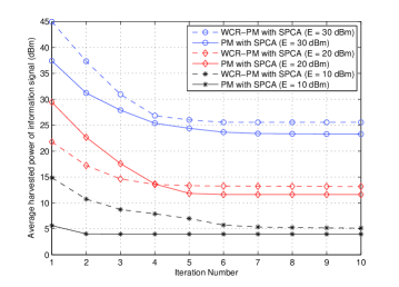
Figure 1: Average transmit power of information signal versus iteration numbers

Fig. 2 illustrates the average transmit power of the information signal in terms of different target secrecy rates with $P=30$ dBm and $\bar{E}_{c,l}=\bar{E}_{e,k}=10$ dBm, $\forall k$. It is observed that the transmit power increases with the secrecy rate target. In addition, the SPCA algorithm achieves the same performance as the 1-D search method, but with much lower complexity. Compared with the scheme without AN, the power consumption of the proposed AN-aided scheme is $9$ dB lower. Moreover, we can check that the proposed scheme performs better than the scheme with $\rho_{c}=\rho_{c,l}=0.5$, and the performance gap becomes larger as the target secrecy rate increases. This indicates that optimizing the PS ratio $\rho_{c,l}$ is important, especially when the target secrecy rate is high.

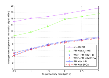
Figure 2: Average transmit power of information signal versus target secrecy rate

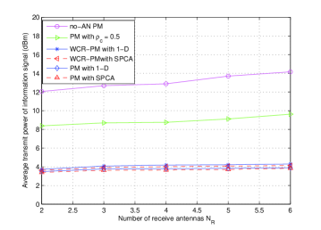
Figure 3: Average transmit power of information signal versus the number of receive antenna at the ERs

In Fig. 3, we compare the average transmit power with respect to different numbers of ER antennas by fixing $N_{T}=8$, $P=40$ dBm, $\bar{E}_{c,l}=\bar{E}_{e,k}=10$ dBm, and $\bar{R}_{c,l}=1$ bps/Hz. In this figure, one can observe that the performance of the 1-D search method and that of the proposed SPCA algorithm remains the same regardless of the value of $N_{R}$. This is due to the fact that all the harvested power at the ERs can be provided by the AN signal.

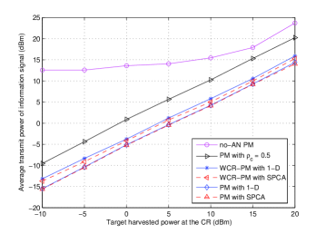
Figure 4: Average transmit power of information signal versus the target harvested power at the CR

In Fig. 4, we plot the average transmit power in terms of different target harvested power at the CR with $P=40$ dBm, $\bar{E}_{e,k}=10$ dBm and $\bar{R}_{c,l}=0.5$ bps/Hz. We can check that the curves of the PM and the WCR-PM schemes increase with the same slope. Moveover, when the harvested power target decreases, the performance gap between the no-AN PM scheme and the proposed PM scheme becomes wider. This indicates that AN is essential in achieving the performance gains. Furthermore, the PM scheme and the WCR-PM scheme require $6$ dB and $4.5$ dB lower power than the PM scheme with fixed $\rho_{c}$, respectively.

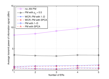
Figure 5: Average transmit power of information signal versus the number of ERs

Fig. 5 evaluates the average transmit power of information signal with respect to different number of ER with $N_{T}=6$, $P=30$ dBm, $\bar{E}_{c,l}=\bar{E}_{e,k}=5$ dBm, and $\bar{R}_{c,l}=1$ bps/Hz. It is observed that both the proposed SPCA algorithms and the 1-D search method achieved the same performance, and the PM with $\rho_{c}=0.5$ exhibits a $2.8$ dBm loss over the scheme with the optimal $\rho_{c,l}^{*}$ regardless of the number of ERs. In addition, we can find that the curve of the no-An PM scheme increases slowly with the number of ERs.

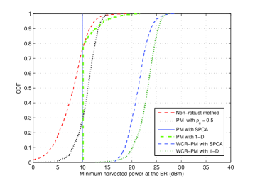
Figure 6: CDF of the minimum harvested power at the ERs

Finally, in Fig. 6 we plot the cumulative density function (CDF) of the minimum harvested power at the ERs with $N_{T}=4$, $P=30$ dBm, $\bar{E}_{c,l}=10$ dBm, $\bar{E}_{e,k}=10$ dBm, $\bar{R}_{c,l}=0.5$ bps/Hz, and $\varepsilon=0.1$. It is observed that the proposed robust schemes always satisfy the predefined harvested power target ($\bar{E}_{e,k}=10$ dBm), whereas the non-robust method achieves only 25% of the predefined harvested power at the ERs.

VII Conclusion

In this paper, we have proposed a transmit beamforming power minimization scheme for a multi-user MIMO SWIPT secrecy communication system where power splitters are employed by the receivers for SWIPT operation. The original problem, which was shown to be non-convex, was relaxed to formulate a two-layer problem. The inner layer problem was recast as a sequence of SDPs and solved accordingly. Then the optimal solution to the outer problem, on the other hand, has been obtained through one-dimensional line search. This optimization framework has also been extended to robust secrecy transmission designs by incorporating deterministic channel uncertainties. Moreover, tightness of the relaxation scheme has been investigated for both the perfect and imperfect CSI cases by showing that the optimal solution is rank-one. To reduce the computational complexity, an SPCA based iterative algorithm has been proposed, which achieved near-optimal solution in both the perfect and imperfect CSI cases. Finally, numerical results have been provided to validate the performance of the proposed transmit beamforming schemes.

Appendix A Proof of Theorem 2

We first consider the Lagrange dual function of (6) as

$$\!\!\!\!\!\!\!\!\!\!\!\!\mathcal{L}(\mathbf{Q},\mathbf{W},\mathbf{Z},\mathbf{Y},\xi_{l},\mathbf{A}_{e,k},\gamma,\mu_{l},\theta_{k})\!=\!\textrm{tr}(\mathbf{Q})-\textrm{tr}(\mathbf{Z}\mathbf{Q})-\textrm{tr}(\mathbf{Y}\mathbf{W})$$

$$\!\!\!\!\!\!\!\!\!\!\!\!-\xi_{l}\bigg{[}\textrm{tr}\bigg{(}\mathbf{h}_{c,l}\mathbf{h}_{c,l}^{H}[t\mathbf{Q}\!-\!(2^{\bar{R}_{c,l}}\!-\!t)\mathbf{W}]\bigg{)}-(2^{\bar{R}_{c,l}}-t)(\sigma_{c,l}^{2}\!+\!\frac{\sigma_{p,l}^{2}}{\rho_{c,l}})\bigg{]}$$

$$\!\!\!\!\!\!\!\!\!\!\!\!-\sum_{k=1}^{K}\textrm{tr}\bigg{[}\mathbf{A}_{e,k}\bigg{(}\mathbf{H}_{e,k}^{H}\big{(}({\frac{1}{t}}\!-\!1)\mathbf{W}-\mathbf{Q}\big{)}\mathbf{H}_{e,k}\!+\!({\frac{1}{t}}\!-\!1)\sigma_{k}^{2}\mathbf{I}\bigg{)}\bigg{]}$$

$$\!\!\!\!\!\!\!\!\!\!\!\!+\gamma\big{(}\textrm{tr}(\mathbf{Q}\!+\!\mathbf{W})\!-\!P\big{)}\!-\!\mu_{l}\bigg{[}\textrm{tr}\big{(}\mathbf{h}_{c,l}\mathbf{h}_{c,l}^{H}(\mathbf{Q}\!+\!\mathbf{W})\big{)}-\frac{\bar{E}_{c,l}}{1\!-\!\rho_{c,l}}\!+\!\sigma_{c,l}^{2}\bigg{]}$$

$$\!\!\!\!\!\!\!\!\!\!\!\!-\sum_{k=1}^{K}\theta_{k}\bigg{(}\textrm{tr}\big{(}\mathbf{H}_{e,k}^{H}(\mathbf{Q}\!+\!\mathbf{W})\mathbf{H}_{e,k}\big{)}-\bar{E}_{e,k}\!+\!N_{R}\sigma_{k}^{2}\bigg{)},$$

where $\mathbf{Z}\in\mathbb{H}_{+}^{N_{T}}$, $\mathbf{Y}\in\mathbb{H}_{+}^{N_{T}}$, $\xi_{l}\in\mathbb{R}_{+}$, $\mathbf{A}_{e,k}\in\mathbb{H}_{+}^{N_{T}}$, $\gamma\in\mathbb{R}_{+}$, $\mu_{l}\in\mathbb{R}_{+}$, and $\theta_{k}$ are the dual variables of $\mathbf{Q}$, $\mathbf{W}$, (6a), (6b), (4e), (4e), and (4e), respectively. Then, some of the related KKT conditions are listed as

$$\!\!\!\!\!\!\!\!\!\!\!\frac{\partial\mathcal{L}}{\partial\mathbf{Q}}=\mathbf{I}-\mathbf{Z}-(\xi_{l}t+\mu_{l})\mathbf{h}_{c,l}\mathbf{h}_{c,l}^{H}+\sum_{k=1}^{K}\mathbf{H}_{e,k}\mathbf{A}_{e,k}\mathbf{H}_{e,k}^{H}$$

$$~{}~{}~{}~{}+\gamma\mathbf{I}-\sum_{k=1}^{K}\theta_{k}\mathbf{H}_{e,k}\mathbf{H}_{e,k}^{H}=\mathbf{0},$$ (55a)

$$\!\!\!\!\!\!\!\!\!\!\!\frac{\partial\mathcal{L}}{\partial\mathbf{W}}\!=\!-\mathbf{Y}\!+\![\xi_{l}(2^{\bar{R}_{c,l}}\!-\!t)\!-\!\mu_{l}]\mathbf{h}_{c,l}\mathbf{h}_{c,l}^{H}+\gamma\mathbf{I}\!-\!\sum_{k=1}^{K}\theta_{k}\mathbf{H}_{e,k}\mathbf{H}_{e,k}^{H}$$

$$~{}~{}~{}~{}\!-\!\sum_{k=1}^{K}({\frac{1}{t}}\!-\!1)\mathbf{H}_{e,k}\mathbf{A}_{e,k}\mathbf{H}_{e,k}^{H}\!=\!\mathbf{0},\!\!\!\!\!\!\!\!$$ (55b)

$$\!\!\!\!\!\!\!\!\!\!\!\mathbf{Z}\mathbf{Q}=\mathbf{0},~{}\mathbf{Y}\!\succeq\!\mathbf{0},~{}\mathbf{A}_{e,k}\succeq\mathbf{0},~{}\xi_{l}\geq 0,~{}\mu_{l}\geq 0,~{}\forall k.\!\!\!\!\!\!\!\!$$ (55c)

From the Lagrangian function and the KKT conditions, we have $0<\rho_{c,l}\leq 1$ and the KKT condition $\xi_{l}>0$ and $\mu_{l}>0$. Now, we will show these conditions via the dual problem of (6) as

$$\!\!\!\!\!\!\!\!\!\!\max_{\mathbf{Z},\mathbf{Y},\mathbf{A}_{e,k},\xi_{l},\gamma,\mu_{l},\theta_{k}}\min_{\mathbf{Q},\mathbf{W},\rho_{c,l}}\mathcal{L}(\mathbf{Q},\mathbf{W},\mathbf{Z},\mathbf{Y},\xi_{l},\mathbf{A}_{e,k},\gamma,\mu_{l})$$

$$= \!\!\!\!\!\!\!\!\!\!\max_{\mathbf{Z},\mathbf{Y},\mathbf{A}_{e,k},\xi_{l},\gamma,\mu_{l},\theta_{k}}\min_{\mathbf{Q},\mathbf{W},\rho_{c,l}}\bigg{[}-\textrm{tr}(\mathbf{Z}\mathbf{Q})\!-\!\textrm{tr}(\mathbf{Y}\mathbf{W})$$

$$\!\!\!\!\!\!\!+\frac{\xi_{l}(2^{\bar{R}_{c,l}}\!-\!t)\sigma_{p,l}^{2}}{\rho_{c,l}}\!+\!\frac{\mu_{l}\bar{E}_{c,l}}{1\!-\!\rho_{c,l}}\!-\!\sum_{k=1}^{K}({\frac{1}{t}}\!-\!1)\sigma_{e}^{2}\textrm{tr}(\mathbf{A}_{e,k})$$

$$\!\!\!\!\!\!+[\xi_{l}(2^{\bar{R}_{c,l}}\!-\!t)\!-\!\mu_{l}]\sigma_{c,l}^{2}\!-\!\gamma P+\sum_{k=1}^{K}\theta_{k}(\bar{E}_{e,k}\!-N_{R}\sigma_{k}^{2})\bigg{]}.$$

Since problem (6) is convex and satisfies the Slater’s condition, the duality gap between (6) and (A) is zero, and the strong duality holds. Therefore solving problem (6) is equivalent to solving (A). In addition, the constraint $0<\rho_{c,l}\leq 1$ can be satisfied as

$$\min_{0<\rho_{c,l}\leq 1}\frac{\xi_{l}(2^{\bar{R}_{c,l}}\!-\!t)\sigma_{p,l}^{2}}{\rho_{c,l}}\!+\!\frac{\mu_{l}\bar{E}_{c,l}}{1\!-\!\rho_{c,l}}.$$

Also the optimal variable $\rho_{c,l}^{*}$, and the dual variables $\xi_{l}^{*},\mu_{l}^{*}$ are related by

$$\rho_{c,l}^{*}\!=\!\frac{\sqrt{\xi_{l}^{*}(2^{\bar{R}_{c,l}}\!-\!t)\sigma_{p,l}^{2}}}{\sqrt{\xi_{l}^{*}(2^{\bar{R}_{c,l}}\!-\!t)\sigma_{p,l}^{2}}\!+\!\sqrt{\mu_{l}^{*}\bar{E}_{c,l}}}.$$

From the above inequality, we will show that $\xi_{l}^{*}>0$ and $\mu_{l}^{*}>0$ by contradiction. Suppose that $\xi_{l}^{*}=0$ and/or $\mu_{l}^{*}=0$. Then there are two cases (i.e., $\rho_{c,l}^{*}=0$ or $1$), which violate the constraints (4e) and (4e). Thus, it follows $\xi_{l}>0$ and $\mu_{l}>0$. Now, subtracting (55b) from (55a) yields

$$\mathbf{Z}\!+\!\xi_{l}^{*}2^{\bar{R}_{c,l}}\mathbf{h}_{c,l}\mathbf{h}_{c,l}^{H}\!=\!\mathbf{I}\!+\!\mathbf{Y}\!+\!{\frac{1}{t}}\sum_{k=1}^{K}\mathbf{H}_{e,k}\mathbf{A}_{e,k}\mathbf{H}_{e,k}^{H}.$$ (57)

We post-multiply $\mathbf{Q}$ by both sides of (57) and use (55c) as

$$\xi_{l}^{*}2^{\bar{R}_{c,l}}\mathbf{h}_{c,l}\mathbf{h}_{c,l}^{H}\mathbf{Q}\!=\!\bigg{(}\!\mathbf{I}\!+\!\mathbf{Y}\!+\!{\frac{1}{t}}\sum_{k=1}^{K}\mathbf{H}_{e,k}\mathbf{A}_{e,k}\mathbf{H}_{e,k}^{H}\!\bigg{)}\mathbf{Q}.$$

Then, it becomes

$$\xi_{l}^{*}2^{\bar{R}_{c,l}}\bigg{(}\mathbf{I}\!+\!\mathbf{Y}\!+\!{\frac{1}{t}}\sum_{k=1}^{K}\mathbf{H}_{e,k}\mathbf{A}_{e,k}\mathbf{H}_{e,k}^{H}\bigg{)}^{-1}\mathbf{h}_{c,l}\mathbf{h}_{c,l}^{H}\mathbf{Q}\!=\!\mathbf{Q}.\!\!\!\!\!\!\!\!\!\!\!\!\!\!\!\!\!\!$$

Due to $\xi_{l}^{*}>0$, we have

$$\begin{split}&\textrm{rank}(\mathbf{Q})\\ =&\textrm{rank}\bigg{[}\xi_{l}^{*}2^{\bar{R}_{c,l}}\bigg{(}\!\mathbf{I}\!+\!\mathbf{Y}\!+\!{\frac{1}{t}}\sum_{k=1}^{K}\mathbf{H}_{e,k}\mathbf{A}_{e,k}\mathbf{H}_{e,k}^{H}\!\bigg{)}^{-1}\mathbf{h}_{c,l}\mathbf{h}_{c,l}^{H}\mathbf{Q}\bigg{]}\\ =&\textrm{rank}(\mathbf{h}_{c,l}\mathbf{h}_{c,l}^{H})\leq\!1.\end{split}$$

This completes the theorem.                                   $\blacksquare$

Appendix B Proof of Theorem 3

First we write the Lagrange dual function of (38) as

$$\begin{split}&\mathcal{L}(\mathbf{Q},\mathbf{W},\mathbf{Z},\mathbf{Y},\xi_{l},\mathbf{T}_{c,l},\mathbf{T}_{e,k},\mathbf{R}_{c,l},\mathbf{R}_{e,k})=\textrm{tr}(\mathbf{Q})-\textrm{tr}(\mathbf{Z}\mathbf{Q})\\ &\!-\!\textrm{tr}(\mathbf{Y}\mathbf{W})\!+\!\xi_{l}\big{(}\textrm{tr}(\mathbf{Q}+\mathbf{W})\!-\!P\big{)}-\textrm{tr}(\mathbf{T}_{c,l}\mathbf{A}_{c,l})\\ &\!-\!\textrm{tr}\bigg{(}\mathbf{T}_{c,l}\mathbf{H}_{c,l}^{H}\big{(}t_{1}\mathbf{Q}\!-\!(2^{\bar{R}_{c,l}}\!-\!t_{1})\mathbf{W}\big{)}\mathbf{H}_{c,l}\bigg{)}-\sum_{k=1}^{K}\textrm{tr}(\mathbf{T}_{e,k}\mathbf{A}_{e,k})\\ &\!-\!\sum_{k=1}^{K}\textrm{tr}\bigg{(}\mathbf{T}_{e,k}\mathbf{G}_{e,k}^{H}\big{(}({\frac{1}{t_{1}}}\!-\!1)\mathbf{W}\!-\mathbf{Q}\big{)}\mathbf{G}_{e,k}\bigg{)}\!-\!\textrm{tr}(\mathbf{R}_{c,l}\mathbf{B}_{c,l})\\ &\!-\!\textrm{tr}\big{(}\mathbf{R}_{c,l}\mathbf{H}_{c,l}^{H}(\mathbf{Q}\!+\!\mathbf{W})\mathbf{H}_{c,l}\big{)}\!-\!\sum_{k=1}^{K}\sum_{j=1}^{N_{R}}\textrm{tr}(\mathbf{R}_{e,k}\mathbf{B}_{e,k})\\ &\!-\sum_{k=1}^{K}\sum_{j=1}^{N_{R}}\textrm{tr}\bigg{(}(\mathbf{Q}\!+\!\mathbf{W})\mathbf{D}_{e,k}^{(j,j)}\bigg{)},\!\!\!\!\!\!\!\end{split}$$

where $\mathbf{Z}\in\mathbb{H}_{+}^{N_{T}}$, $\mathbf{Y}\in\mathbb{H}_{+}^{N_{T}}$, $\xi_{l}\in\mathbb{R}_{+}$, $\mathbf{T}_{c,l}\in\mathbb{H}_{+}^{N_{T}}$, $\mathbf{T}_{e,k}\in\mathbb{H}_{+}^{N_{T}}$, $\mathbf{R}_{c,l}\in\mathbb{H}_{+}^{N_{T}}$, and $\mathbf{R}_{e,k}\in\mathbb{H}_{+}^{N_{T}N_{R}}$ are the dual variables of $\mathbf{Q}$, $\mathbf{W}$, (28), (37), (29c), and (29f), respectively, and

$$\!\!\!\!\!\!\!\!\!\!\!\!\!\mathbf{A}_{c,l}\!=\!\left[\!\!\begin{array}[]{cc}\lambda_{c,l}\mathbf{I}\!&\!\mathbf{0}_{N_{T}\times 1}\\ \mathbf{0}^{H}_{1\times N_{T}}\!&\!-(2^{\bar{R}_{c,l}}\!-\!t_{1})(\sigma_{c,l}^{2}\!+\!a\sigma_{p,l}^{2})\!-\!\lambda_{c,l}\varepsilon_{c,l}^{2},\end{array}\!\!\right],$$ (60)

$$\!\!\!\!\!\!\!\!\!\!\!\!\!\mathbf{A}_{e,k}\!=\!\left[\begin{array}[]{cc}(({\frac{1}{t_{1}}}-1)\sigma_{k}^{2}\!-\!\lambda_{e,k})\mathbf{I}\!&\!\mathbf{0}_{N_{T}\times 1}\\ \mathbf{0}^{H}_{1\times N_{T}}\!&\!\frac{\lambda_{e,k}}{\varepsilon_{e,k}^{2}}\mathbf{I}\end{array}\right]\!\!,\mathbf{G}_{e,k}\!=\!\left[\begin{array}[]{cc}\mathbf{\bar{H}}_{e,k}\!&\!\mathbf{I}\end{array}\right],$$ (64)

$$\!\!\!\!\!\!\!\!\!\!\!\!\!\mathbf{B}_{c,l}\!=\!\left[\begin{array}[]{cc}\alpha_{c,l}\mathbf{I}\!&\!\mathbf{0}_{N_{T}\times 1}\\ \mathbf{0}^{H}_{1\times N_{T}}\!&\!\sigma_{c,l}^{2}\!-\!b\bar{E}_{c,l}\!-\!\alpha_{c,l}\varepsilon_{c,l}^{2}\end{array}\right]\!\!,\mathbf{{\hat{H}}}_{e,k}\!=\!\left[\!\!\begin{array}[]{cc}\mathbf{I}\!&\!\mathbf{\bar{h}}_{e,k}\end{array}\!\!\right],$$ (68)

$$\!\!\!\!\!\!\!\!\!\!\!\!\!\mathbf{B}_{e,k}\!=\!\left[\!\!\begin{array}[]{cc}\alpha_{e,k}\mathbf{I}\!&\!\mathbf{0}_{N^{2}_{T}\times 1}\\ \mathbf{0}^{H}_{1\times N^{2}_{T}}\!&\!-\bar{E}_{e,k}\!+\!N_{R}\sigma_{k}^{2}\!-\!\alpha_{e,k}\varepsilon_{e,k}^{2}\end{array}\!\!\right]\!\!,\mathbf{H}_{c,l}\!=\!\left[\!\!\begin{array}[]{cc}\mathbf{I}\!&\!\mathbf{\bar{h}}_{c,l}\end{array}\!\!\right],$$ (72)

and $\mathbf{D}_{e,k}^{(j,j)}\in\mathbb{H}_{+}^{N_{T}}$ is a block submatrix of $\mathbf{\hat{H}}_{e,k}\mathbf{R}_{e,k}\mathbf{\hat{H}}_{e,k}^{H}$ as

$$\mathbf{\hat{H}}_{e,k}\mathbf{R}_{e,k}\mathbf{\hat{H}}_{e,k}^{H}\!=\!\left[\!\!\begin{array}[]{ccc}\mathbf{D}^{(1,1)}_{e,k}\!&\!\cdots\!&\!\mathbf{D}^{(1,N_{R})}_{e,k}\\ \vdots\!&\!\ddots\!&\!\vdots\\ \mathbf{D}^{(N_{R},1)}_{e,k}\!&\!\cdots\!&\!\mathbf{D}^{(N_{R},N_{R})}_{e,k}\end{array}\!\!\right],\forall k.\\$$

Now, we consider the following related KKT conditions as

$$\!\!\!\!\!\!\!\frac{\partial\mathcal{L}}{\partial\mathbf{Q}}=\mathbf{I}-\mathbf{Z}+\xi_{l}\mathbf{I}-t_{1}\mathbf{H}_{c,l}\mathbf{T}_{c,l}\mathbf{H}_{c,l}^{H}+\sum_{k=1}^{K}\mathbf{G}_{e,k}\mathbf{T}_{e,k}\mathbf{G}_{e,k}^{H}$$

$$\!\!\!\!\!\!\!~{}~{}~{}~{}~{}~{}-\mathbf{H}_{c,l}\mathbf{R}_{c,l}\mathbf{H}_{c,l}^{H}-\sum_{k=1}^{K}\sum_{j=1}^{N_{R}}\mathbf{D}_{e,k}^{(j,j)}=\mathbf{0},$$ (73a)

$$\!\!\!\!\!\!\!\frac{\partial\mathcal{L}}{\partial\mathbf{W}}=-\mathbf{Y}+\xi_{l}\mathbf{I}+(2^{\bar{R}_{c,l}}-t_{1})\mathbf{H}_{c,l}\mathbf{T}_{c,l}\mathbf{H}_{c,l}^{H}$$

$$\!\!\!\!\!\!\!~{}~{}~{}~{}~{}~{}-\sum_{k=1}^{K}({\frac{1}{t_{1}}}-1)\mathbf{G}_{e,k}\mathbf{T}_{e,k}\mathbf{G}_{e,k}^{H}-\mathbf{H}_{c,l}\mathbf{R}_{c,l}\mathbf{H}_{c,l}^{H}$$

$$\!\!\!\!\!\!\!~{}~{}~{}~{}~{}~{}-\sum_{k=1}^{K}\sum_{j=1}^{N_{T}}\mathbf{D}_{e,k}^{(j,j)}=\mathbf{0},$$ (73b)

$$\!\!\!\!\!\!\!~{}~{}\mathbf{Q}\mathbf{Z}=\mathbf{0},~{}\mathbf{W}\succeq\mathbf{0},$$ (73c)

$$\!\!\!\!\!\!\!~{}\big{(}\mathbf{A}_{c,l}+\mathbf{H}_{c,l}^{H}\big{(}t_{1}\mathbf{Q}-(2^{\bar{R}_{c,l}}-t_{1})\mathbf{W}\big{)}\mathbf{H}_{c,l}\big{)}\mathbf{T}_{c,l}=\mathbf{0}.$$ (73d)

Subtracting (73b) from (73a) generates

$$\mathbf{I}\!-\!\mathbf{Z}\!+\!\mathbf{Y}\!-\!2^{\bar{R}_{c,l}}\mathbf{H}_{c,l}\mathbf{T}_{c,l}\mathbf{H}_{c,l}^{H}\!+\!\sum_{k=1}^{K}{\frac{1}{t_{1}}}\mathbf{G}_{e,k}\mathbf{T}_{e,k}\mathbf{G}_{e,k}^{H}\!=\!\mathbf{0},$$

and it follows

$$\mathbf{Z}\!+\!2^{\bar{R}_{c,l}}\mathbf{H}_{c,l}\mathbf{T}_{c,l}\mathbf{H}_{c,l}^{H}\!=\!\mathbf{I}+\mathbf{Y}+\sum_{k=1}^{K}{\frac{1}{t_{1}}}\mathbf{G}_{e,k}\mathbf{T}_{e,k}\mathbf{G}_{e,k}^{H}.$$

Pre-multiplying both sides of the above equality by $\mathbf{Q}$ and applying the inverse yields

$$2^{\bar{R}_{c,l}}\mathbf{Q}\mathbf{H}_{c,l}\mathbf{T}_{c,l}\mathbf{H}_{c,l}^{H}\bigg{(}\mathbf{I}\!+\!\mathbf{Y}\!+\!\sum_{k=1}^{K}{\frac{1}{t_{1}}}\mathbf{G}_{e,k}\mathbf{T}_{e,k}\mathbf{G}_{e,k}^{H}\bigg{)}^{-1}\!\!\!=\!\mathbf{Q}.$$

Hence, we have the rank relation as

$$\begin{split}&\textrm{rank}(\mathbf{Q})\\ =~{}&\textrm{rank}\bigg{(}2^{\bar{R}_{c,l}}\mathbf{Q}\mathbf{H}_{c,l}\mathbf{T}_{c,l}\mathbf{H}_{c,l}^{H}\big{(}\mathbf{I}\!+\!\mathbf{Y}\!+\!\sum_{k=1}^{K}{\frac{1}{t_{1}}}\mathbf{G}_{e,k}\mathbf{T}_{e,k}\mathbf{G}_{e,k}^{H}\big{)}^{-1}\bigg{)}\\ \leq~{}&\textrm{rank}(\mathbf{H}_{c,l}\mathbf{T}_{c,l}\mathbf{H}_{c,l}^{H}).\end{split}$$ (74)

Now, we will compute the rank of the matrix $\mathbf{H}_{c,l}\mathbf{T}_{c,l}\mathbf{H}_{c,l}^{H}$. To this end, we consider the following two equalities as

$$\left[\!\!\begin{array}[]{cc}\mathbf{I}\!&\!\mathbf{0}\end{array}\!\!\right]\mathbf{H}_{c,l}^{H}\!=\!\mathbf{I},$$ (76)

$$\left[\!\!\begin{array}[]{cc}\mathbf{I}\!&\!\mathbf{0}\end{array}\!\!\right]\mathbf{A}_{c,l}\!=\!\lambda_{c,l}\bigg{(}\mathbf{H}_{c,l}\!-\!\left[\!\!\begin{array}[]{cc}\mathbf{0}\!&\!\mathbf{\bar{h}}_{c,l}\end{array}\!\!\right]\bigg{)}.$$ (79)

Pre-multiplying $\left[\begin{array}[]{cc}\mathbf{I}&\mathbf{0}\end{array}\right]$ and post-multiplying $\mathbf{H}_{c,l}^{H}$ to (73d), it follows

$$\begin{split}&\left[\!\!\begin{array}[]{cc}\mathbf{I}\!&\!\mathbf{0}\end{array}\!\!\right]\mathbf{A}_{c,l}\mathbf{T}_{c,l}\mathbf{H}_{c,l}^{H}\\ &~{}-\left[\!\!\begin{array}[]{cc}\mathbf{I}\!&\!\mathbf{0}\end{array}\!\!\right]\mathbf{H}_{c,l}^{H}\big{(}t_{1}\mathbf{Q}\!-\!(2^{\bar{R}_{c,l}}\!-\!t_{1})\mathbf{W}\big{)}\mathbf{H}_{c,l}\mathbf{T}_{c,l}\mathbf{H}_{c,l}^{H}\!=\!\mathbf{0},\end{split}$$

and thus we get

$$\begin{split}&\big{(}\lambda_{c,l}\mathbf{I}\!+\!t_{1}\mathbf{Q}-(2^{\bar{R}_{c,l}}-t_{1})\mathbf{W}\big{)}\mathbf{H}_{c,l}\mathbf{T}_{c,l}\mathbf{H}_{c,l}^{H}\\ &=\lambda_{c,l}\left[\!\!\begin{array}[]{cc}\mathbf{0}\!&\!\mathbf{\bar{h}}_{c,l}\end{array}\!\!\right]\mathbf{T}_{c,l}\mathbf{H}_{c,l}^{H}.\end{split}$$

It is easily verified that $\lambda_{c,l}\mathbf{I}+t_{1}\mathbf{Q}-(2^{\bar{R}_{c,l}}-t_{1})\mathbf{W}\succeq\mathbf{0}$ and it is non-singular. Thus multiplying this matrix will not change the rank of the resulting matrix, and we obtain

$$\begin{split}&\textrm{rank}(\mathbf{H}_{c,l}\mathbf{T}_{c,l}\mathbf{H}_{c,l}^{H})\\ =~{}&\textrm{rank}\bigg{(}\!\big{(}\!\lambda_{c,l}\mathbf{I}\!+\!t_{1}\mathbf{Q}\!-\!(2^{\bar{R}_{c,l}}\!-\!t_{1})\mathbf{W}\!\big{)}\mathbf{H}_{c,l}\mathbf{T}_{c,l}\mathbf{H}_{c,l}^{H}\!\bigg{)}\\ =~{}&\textrm{rank}\bigg{(}\!\lambda_{c,l}\left[\!\begin{array}[]{cc}\mathbf{0}\!&\!\mathbf{\bar{h}}_{c,l}\end{array}\!\right]\mathbf{T}_{c,l}\mathbf{H}_{c,l}^{H}\!\bigg{)}\\ \leq~{}&\textrm{rank}\bigg{(}\!\left[\!\!\begin{array}[]{cc}\mathbf{0}\!&\!\mathbf{\bar{h}}_{c,l}\end{array}\!\!\right]\!\bigg{)}\!\leq\!1.\end{split}$$ (80)

This completes the proof of Theorem 3.                                    $\blacksquare$

References

• [1] L. R. Varshney, “Transporting information and energy simultaneously,” in Proc. IEEE ISIT, pp. 1612-1616, Jul. 2008.
• [2] S. Bi, C. K. Ho, and R. Zhang, “Wireless powered communication: opportunities and challenges,” IEEE Commun. Mag., vol. 53, no. 4, pp. 117-125, Apr. 2015.
• [3] Z. Ding, C. Zhong, D. W. K. Ng, M. Peng, H. A. Suraweera, R. Schober, and H. V. Poor, “Application of smart antenna technologies in simultaneous wireless information and power transfer,” IEEE Commun. Mag., vol. 53, no. 4, pp. 86-93, Apr. 2015.
• [4] D. W. K. Ng, E. S. Lo, and R. Schober, “Energy-effcient resource allocation in OFDMA systems with hybrid energy harvesting base station,” IEEE Trans. Wireless Commun., vol. 12, no. 7, pp. 3412-3427, Jul. 2013.
• [5] R. Zhang and C. Ho, “MIMO broadcasting for simultaneous wireless information and power transfer,” IEEE Trans. Wireless Commun., vol. 12, no. 5, pp. 1989-2001, May 2013.
• [6] Z. Zhu, K.-J. Lee, Z. Wang, and I. Lee. “Robust beamforming and power splitting design in distributed antenna system with SWIPT under bounded channel uncertainty,” in Proc. IEEE VTC spring, pp. 1-5, May 2015.
• [7] H. Lee, S.-R. Lee, K.-J. Lee, and I. Lee, “Optimal beamforming designs for wireless information and power transfer in MISO interference channels,” IEEE Trans. Wireless Commun., vol. 14, no. 9, pp. 4810-4821, Sep. 2015.
• [8] Z. Zhu, Z. Chu, Z. Wang, and I. Lee, “Robust beamforming design for MISO secrecy multicasting systems with energy harvesting,” in Proc. IEEE VTC Spring, pp. 1-5, May 2016.
• [9] Z. Zhu, Z. Wang, K.-J. Lee, Z. Chu, and I. Lee, “Robust transceiver designs in multiuser MISO broadcasting with simultaneous wireless information and power transmission,” Journal of Commun. and Networks, vol. 18, no. 2, pp. 173-181, Apr. 2016.
• [10] L. Dong, Z. Han, A. P. Petropulu, and H. V. Poor, “Improving wireless physical layer security via cooperating relays,” IEEE Trans. Signal Process., vol. 58, no. 3, pp. 1875-1888, Mar. 2010.
• [11] Z. Chu, H. Xing, M. Johnston, and S. Le Goff, “Secrecy rate optimizations for a MISO secrecy channel with multiple multi-antenna eavesdroppers,” IEEE Trans. Wireless Commun., vol. 15, no. 1, pp. 283-297, Jan. 2016.
• [12] A. Khisti and G. W. Wornell, “Secure transmission with multiple antennas I: The MISOME wiretap channel,” IEEE Trans. Inform. Theory, vol. 56, no. 7, pp. 3088-3104, Nov. 2010.
• [13] Z. Chu, K. Cumanan, Z. Ding, M. Johnston, and S. Y. Le Goff, “Secrecy rate optimizations for a MIMO secrecy channel with a cooperative jammer,” IEEE Trans. Vehicular Technol., vol. 64, no. 5, pp. 1833-1847, May 2015.
• [14] Q. Li, Q. Zhang, and J. Qin, “Secure relay beamforming for SWIPT in amplify-and-forward two-way relay networks,” IEEE Trans. Vehicular Technol., vol. 65, no. 11, pp. 9006-9019, Nov. 2016.
• [15] S. Goel and R. Negi, “Guaranteeing secrecy using artificial noise,” IEEE Trans. Wireless Commun., vol. 7, no. 6, pp. 2180-2189, Jun. 2008.
• [16] Q. Li and W.-K. Ma, “Spatially selective artificial-noise aided transmit optimization for MISO multi-eves secrecy rate maximization,” IEEE Trans. Signal Process., vol. 61, no. 10, pp. 2704-2717, May 2013.
• [17] L. Liu, R. Zhang, and K.-C. Chua, “Secrecy wireless information and power transfer with MISO beamforming,” IEEE Trans. Signal Process., vol. 62, no. 7, pp. 1850-1863, Apr. 2014.
• [18] M. Khandaker and K. Wong, “Masked beamforming in the presence of energy-harvesting eavesdroppers,” IEEE Trans. Inf. Forensics Security, vol. 10, pp. 40-54, Jan. 2015.
• [19] Q. Shi, W. Xu, J. Wu; E. Song, and Y. Wang, “Secure beamforming for MIMO broadcasting with wireless information and power transfer,” IEEE Trans. Wireless Commun., vol. 14, no. 5, pp. 2841-2853, May 2015.
• [20] D. W. K. Ng, E. S. Lo, and R. Schober, “Robust beamforming for secure communication in systems with wireless information and power transfer,” IEEE Trans. Wireless Commun., vol. 13, no. 8, pp. 4599-4615, Aug. 2014.
• [21] M. Tian, X. Huang, Q. Zhang, and J. Qin, “Robust AN-aided secure transmission scheme in MISO channels with simultaneous wireless information and power transfer,” IEEE Signal Process. Lett., vol. 22, no. 6, pp. 723-727, Jun. 2015
• [22] Z. Chu, Z. Zhu, M. Johnston, and S. L. Goff, “Simultaneous wireless information power transfer for MISO secrecy channel,” IEEE Trans. Vehicular Technol., vol. 15, no. 1, pp. 283-297, Jan. 2016.
• [23] Z. Zhu, Z. Chu, Z. Wang, I. Lee, “Joint optimization of AN-aided beamforming and power splitting designs for MISO secrecy channel with SWIPT,” in Proc. IEEE ICC, pp. 1-6, May. 2016.
• [24] Y. Wang, R. Sun, and X. Wang, “Transceiver design to maximize the weighted sum secrecy rate in full-duplex SWIPT systems,” IEEE Signal Process. Lett., vol. 23, no. 6, pp. 883-887, Jun. 2016.
• [25] J. Xiong, D. Ma, K. Wong, and J. Wei, “Robust masked beamforming for MISO cognitive radio networks with unknown eavesdroppers,” IEEE Trans. Vehicular Technol., vol. 65, no. 2, pp. 744-755, Feb. 2016.
• [26] S. Leng, D. Ng, and R. Schober, “Power efficient and secure multiuser communication systems with wireless information and power transfer,” in Proc. IEEE ICC, pp. 800-806, Jun. 2014.
• [27] S. Mohammadkhani, S. M. Razavizadeh, and I. Lee, “Robust filter and forward relay beamforming with spherical channel state information uncertainties,” in Proc. IEEE ICC, pp. 5023-5028. Jun. 2014.
• [28] S. Boyd and L. Vandenberghe, Convex Optimization. Cambridge, UK: Cambridge University Press, 2004.
• [29] K.-Y. Wang, A. Man-Cho So, T.-H. Chang, W.-K. Ma, and C.-Y. Chi, “Outage constrained robust transmit optimization for multiuser MISO downlinks: tractable approximations by conic optimization,” IEEE Trans. Signal Process., vol. 62, no. 21, pp. 5690-5705, Nov. 2014.
• [30] K. B. Petersern and M. S. Pedersern, The Matrix Cookbook, Nov. 2008 [Online]. Available: http://matrixcookbook.com
• [31] M. Grant and S. Boyd., “CVX: Matlab software for disciplined convex programming,” version 2.0 beta, Available: http://cvxr.com/cvx, Sep. 2012.
• [32] A. Beck, A. Ben-Tal, and L. Tetruashvili, “A sequential parametric convex approximation method with applications to nonconvex truss topology design problems,” J. Global Optim., vol. 47, no. 1, pp. 29-51, May 2010.
• [33] A. S. Vishwanathan, A. J. Smola, and S. V. N. Vishwanathan, “Kernel methods for missing variables,” in Proc. 10th Int. Workshop Artif. Intell. Stat., pp. 325-332, Jan. 2005.
• [34] M. Bengtsson and B. Ottersten, “Optimum and suboptimum transmit beamforming,” in Handbook of Antennas in Wireless Communications, L. C. Godara, Ed., CRC Press, Aug. 2001.
• [35] Z. Zhu, Z. Chu, Z. Wang, and I. Lee, “Outage constrained robust beamforming for secure broadcasting systems with energy harvesting,” IEEE Trans. Wireless Commun., vol. 15, no. 11, pp. 7610-7620, Nov. 2016.
• [36] H. Wang, S. Ma, T.-S. Ng, and H. V. Poor, “A general analytical approach for opportunistic cooperative systems with spatially random relays,” IEEE Trans. Wireless Commun., vol. 10, no. 12, pp. 4122-4129, Dec. 2011.
• [37] E. Karipidis, N. D. Sidiropoulos, and Z.-Q. Luo, “Far-field multicast beamforming for uniform linear antenna arrays,” IEEE Trans. Signal Process., vol. 55, no. 10, pp. 4916-4927, Oct. 2007.