Abstract

Although comparatively bright, the cataclysmic variable GY Hya has not attracted much attention in the past. As part of a project to better characterize such systems photometrically, we observed light curves in white light, each spanning several hours, at Bronberg Observatory, South Africa, in 2004 and 2005, and at the Observatório do Pico dos Dias, Brazil, in 2014 and 2016. These data permit to study orbital modulations and their variations from season to season. The orbital period, already known from spectroscopic observations of Peters & Thorstensen (2005), is confirmed through strong ellipsoidal variations of the mass donor star in the system and the presence of eclipses of both components. A refined period of 0.34723972 (6) days and revised ephemeries are derived. Seasonal changes in the average orbital light curve can qualitatively be explained by variations of the contribution of a hot spot to the system light together with changes of the disk radius. The amplitude of the ellipsoidal variations and the eclipse contact phases permit to put some constraints on the mass ratio, orbital inclination and the relative brightness of the primary and secondary components. There are some indications that the disk radius during quiescence, expressed in units of the component separation, is smaller than in other dwarf novae.

Keywords: Stars: binaries: close – Stars: novae, cataclysmic variables – Stars: dwarf novae – Stars: individual: GY Hya

1 Introduction

Cataclysmic variables (CVs) are binary stars where a Roche-lobe filling late-type component (the secondary) transfers matter via an accretion disk to a white dwarf primary. It may be surprising that even after decades of intense studies of CVs there are still an appreciable number of known or suspected systems, bright enough to be easily observed with comparatively small telescopes, which have not been studied sufficiently for basic parameters to be known with certainty. In some cases even their very class membership still requires confirmation.

Therefore, a small observing project aimed at a better understanding of these stars was initiated in 2014 at the Observatório do Pico dos Dias (OPD), operated by the Laboratório Nacional de Astrofísica, Brazil, using 60cm class telescopes. First results have been published by Bruch (2016, 2017) and Bruch & Diaz (2017). Here, we present time resolved photometry of the long period dwarf nova GY Hya in order to characterize orbital modulations.

Hoffmeister (1963) classified GY Hya as either a RR Lyr or U Gem star. Describing spectroscopic observations, Bond & Tifft (1974) reject the first alternative and consider the U Gem classification as probably correct. This is supported by the spectrum reproduced by Zwitter & Munari (1996) which shows the Balmer series strongly in emission. He I lines are also present. As an indication for the secondary star, the Na D lines are clearly visible in absorption. However, unlike normally seen in quiescent dwarf novae, the He II $\lambda$ 4686 Å  emission line (and the adjacent NIII-OIII complex) is particularly strong. This is more typically the hallmark of magnetic cataclysmic variables, some novalike variables and novae in quiescence (see e.g. Williams 1983). But Cropper (1986) did not find the light of GY Hya to be significantly polarized.

The presence of the secondary star in the spectrum was confirmed by means of time resolved spectroscopy performed by Peters & Thorstensen (2005) who measured the orbital period to be 0.347237 days. Quoting a private communication from one of us (B. Monard) they also mention the presence of eclipses with the same period in the light curve. This is based on data analyzed in more detail in the present contribution.

This study is organized as follows: In Sect. 2 the observations and data reduction techniques are briefly presented. Sect. 3 then deals with the results of the observations which are subsequently discussed in Sect. 4. Finally, a short summary in Sect. 5 concludes this paper.

2 Observations and data reductions

GY Hya was observed at the Centre of Backyard Astronomy (CBA), Pretoria (Bronberg Observatory), in 2002, 2004 and 2005, and at OPD in 2014 and 2016. The observations performed at OPD were obtained at the 0.6-m Zeiss and the 0.6-m Boller & Chivens telescopes. Time series imaging of the field around the target star was performed using cameras of type Andor iKon-L936-B and iKon-L936-EX2 equipped with back illuminated, visually optimized CCDs. Aiming to resolve the expected rapid flickering variations the integration times were kept short. Together with the small readout times of the detectors this resulted in a time resolution of the order of $5^{\raisebox{0.90417pt}{\scriptsize s}}$. In order to maximize the count rates in these short time intervals no filters were used. The observations at CBA were also obtained in white light, using a Meade 30cm LX200 telescope equiped with a SBIG ST7 detector and focal reducer. The time resolution of the light curves was $\sim$60 sec in 2002 and $\sim$30 sec in 2004 and 2005. A summary of the observations is given in Table 1. Some light curve contain gaps caused by intermittent clouds or technical reasons.

Table 1: Journal of observations of GY Hya

Date	Start	End	Obs.*	mean
	(UT)	(UT)		mag**
2002 Mar 06/07	23:31	23:21	BO	15.3
2002 Apr 20/21	17:45	21:31	BO	15.3
2002 Apr 22	16:51	19:33	BO	15.3
2002 May 09	17:20	19:59	BO	15.3
2002 May 27	19:12	22:45	BO	15.3
2004 May 13/14	16:29	21:18	BO	14.5
2004 May 22/23	16:16	21:11	BO	15.3
2004 Jun 04	18:22	23:26	BO	15.3
2004 Jun 06	16:23	19:06	BO	15.4
2005 Apr 11/12	21:26	23:31	BO	15.2
2014 May 01	20:46	21:29	OPD	15.8
2014 May 03	23:26	24:50	OPD	15.8
2014 Jun 19/20	21:17	22:07	OPD	15.8
2014 Jun 21/22	21:38	22:07	OPD	15.9
2016 Apr 06	26:13	28:27	OPD	15.8
2016 Arp 07	26:43	28:31	OPD	15.9
2016 Apr 08	26:18	28:32	OPD	15.9
2016 May 10	22:03	24:10	OPD	16.0
2016 May 11/12	22:09	25:32	OPD	15.8
2016 May 12/13	21:34	20:15	OPD	15.9
2016 Jun 09	20:26	23:54	OPD	15.8
2016 Jun 28/29	21:10	20:56	OPD	15.8
*BOD = Bronberg Observatory
**OPD = Observatório do Pico dos Dias
** $R$ for BO; $V$ for OPD

Since all observations were performed in white light, it was not possible to calibrate the stellar magnitudes. Instead, the brightness was measured as the magnitude difference between the target and the nearby comparison star. For the OPD data, UCAC4 321-074490 ($V=11.901$; Zacharias et al. 1993) was chosen as comparison star. For the CBA data it was UCAC4 321-074480 ($R=13.3$) Their constancy was verified through the observations of check stars. A rough estimate of the effective wavelength of the white light band pass, assuming a mean atmospheric extinction curve, a flat transmission curve for the telescope, and a detector efficiency curve as provided by the manufacturer, yields $\lambda_{\rm eff}\approx 5530$ Å for the OPD instrumentation, very close to the effective wavelength of the Johnson $V$ band (5500 Å; Allen 1973). The detector sensitivity of the CCD used at CBA leads to an effective wavelength close to that of the $R$ band. Therefore, using the known magnitudes of the comparison star it is possible to calculate approximate mean nightly magnitudes of the target star. These are included in Table 1. Assuming that the quiescent brightness of GY Hya did not change significantly the difference of $\approx$$0^{\raisebox{0.90417pt}{\scriptsize m}}_{\raisebox{1.80835pt}{\hskip 1.18999pt.}}5$ between the OPD $V$ band and the CBA $R$ band observations is quite normal for a CV with a dominant contribution from the secondary star (see Sect. 4).

Data reduction of the CBA data and the construction of light curves was done using AIP dataprocessing software. Basic data reduction (biasing, flat-fielding) of the OPD data was performed using IRAF. Light curves were derived with aperture photometry routines implemented in the MIRA software system (Bruch 1993). The latter system was also used for all further data reductions and calculations. Throughout this paper time is expressed in UT. However, whenever observations taken in different nights were combined (e.g., to search for orbital variations) time was transformed into barycentric Julian Date on the Barycentric Dynamical Time (TDB) scale using the online tool provided by Eastman et al. (2010) in order to take into account variations of the light travel time within the solar system.

3 Results

The long term light curve of GY Hya based on data of the American Association of Variable Star Observers (AAVSO) is shown in Fig. 1 (one low data point marked as uncertain has been rejected). Several high points may be interpreted as outbursts and thus corroborate the spectroscopic classification of the system as a dwarf nova. On the other hand GY Hya also occasionally drops into a state of low brightness (but see the discussion in Sect. 4). Interestingly, the system magnitude (disregarding outbursts and low states) seems to decline steadily from $\sim$$15^{\raisebox{0.90417pt}{\scriptsize m}}$ to $\sim$$15^{\raisebox{0.90417pt}{\scriptsize m}}_{\raisebox{1.80835pt}{\hskip 1.18999pt.}}6$ between 1998 and 2005 and remains stable thereafter.

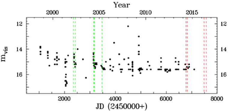
Figure 1: Long term light curve of GY Hya based on AAVSO data. The broken lines delimit the epochs of the time resolved CBA (green) and OPD (red) observations. (For interpretation of the references to colour in this figure legend, the reader is referred to the web version of this article.)

3.1 The orbital light curve

The epochs of our time resolved observations are delimited by broken red (OPD data) and green (CBA data) vertical lines in Fig. 1. As an example, the data of 2016, June 9/10 are shown in Fig. 2. Pronounced variations on hourly time scales are seen, interrupted by an eclipse (the egress of which only being partially observed due to intermittent clouds). Flickering is clearly present, but only on a low level, hardly standing out against the data noise.

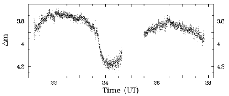
Figure 2: Light curve of GY Hya of 2016, June 9/10.

The long orbital period makes it difficult to observe a continuous light curve covering all phases. However, stitching together data from various nights it is possible to construct a mean orbital light curve. In order to take into account possible night-to-night variations, in an interactive process the mean magnitude difference between the phase folded nightly data and the respective phase range of the average orbital light curve was calculated and subtracted.

Mean orbital light curves were constructed from the observations during each year. The corresponding time base spans between 0.5 and 3 month. The mean curves are shown in Fig. 3, binned in phase intervals of 0.01 (2002 and 2004) and 0.005 (2014 and 2016), respectively. Mid-eclipse according to the revised ephemeris (see Sect. 3.2) has been chosen as phase 0. Since in 2005 GY Hya was observed only in one night, not covering all phases, these data are not regarded here. Moreover, the light curve on 2004, May 13 was not used because the star was in a brighter state at this epoch (see Sect. 3.3).

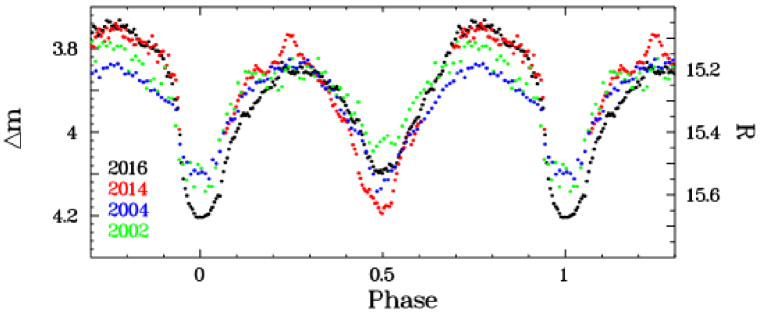
Figure 3: Average orbital light curves of GY Hya in different years. The left scale refers to the differential magnitudes of 2014 and 2016, the right one to those of 2002 and 2004, expressed as approximate $R$ magnitudes. (For visualization of the colours used in this figure, the reader is referred to the web version of this article.)

In general terms, the orbital light curve is characterized by two strongly expressed minima and maxima. The secondary minimum close to phase 0.5 is – depending on the epoch – almost as deep as the primary minimum, while the maximum after the primary minimum is slightly fainter than that after the secondary minimum. However, there are differences from epoch to epoch. This is most evident comparing the year 2004 (blue curve in Fig. 3), when both minima were of equal depth and both maxima of equal height, with 2016 (black curve), when the strongest differences of both, the minima and the maxima, are observed and the primary minimum is deepest. In 2014 the secondary minimum reached almost the depth of the primary minimum in 2016. Unfortunately, the primary minimum was not covered in that year.

3.2 Ephemeris

The spectroscopic period measured by Peters & Thorstensen (2005) and the photometric period quoted by them rely on a comparatively short time base. Combining the new observations of 2014 and 2016 with the those of 2002 – 2005 enlarges significantly the time base for the precise determination of the orbital period. Instead of measuring individual eclipse times a representative minimum epoch for each observing season was derived from the average orbital light curves of each year. Only for 2005, with just one partial light curve available, the minimum epoch was measured directly. To best determine the location of the bottom of the eclipse, polynomials of various degrees (between 2 – 5) and a Gaussian were fitted to the eclipse profile and the epoch of the respective extrema calculated. Their mean values together with their standard deviations are listed in Table 2. A linear least squares fit to these data yields the updated ephemeris:

$${\rm BJD_{min}}=2457484.2337(7)+0.34723972(6)\times E$$

Here $E$ is the cycle number. The quoted uncertainties are formal fit errors which may underestimate the true error. The distribution of data points within two restricted time intervals separated by more than a decade does not allow to determine a possible period derivative. Therefore, only a linear ephemeries, i.e., the average period over the total time base, is given.

Table 2: GY Hya eclipse epochs

Year	Cycle No.	Eclipse epoch
		BJD (TDB)
2002	-14 785	2 452 350.2959 $\pm$ 0.0018
2004	-12 487	2 453 148.2508 $\pm$ 0.0018
2005	-11 554	2 453 472.2248 $\pm$ 0.0007
2016	-12 480	2 457 484.2340 $\pm$ 0.0007

3.3 Outburst light curve

On 2004, May 13/14 GY Hya was observed to be $0^{\raisebox{0.90417pt}{\scriptsize m}}_{\raisebox{1.80835pt}{\hskip 1.18999pt.}}8$ brighter than normal. The long-term AAVSO light curves shows that it has been at about the same brightness level for at least 3 days around this date. Nine days later the normal quiescent level is reached again. Although the sparse data do not permit to say if the late phase of a genuine dwarf nova outburst has been observed, for simplicity we will subsequently refer to this high state as an outburst. The shape of the outburst orbital light curve, shown in black in Fig. 4, is drastically different from the average (quiescent state) curve during the other observing nights of the same year, shown in red in the figure. While the bottom of the primary minimum (the eclipse) attains the same magnitude in both states the amplitude of the eclipse is much larger during outburst. The width of the eclipse in both states, indicated by the broken vertical lines in the figure, is very similar ($\Delta\phi=0.140$); at most the eclipse may start slightly earlier during outburst. It is “V”-shaped in outburst but flat bottomed during quiescence.

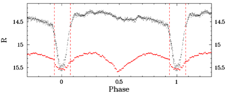
Figure 4: Light curve of GY Hya of 2004, May 13/14, observed during an outburst, folded on the orbital period (black) together with the average quiescent orbital light curve of 2004 (red). (For interpretation of the references to colour in this figure legend, the reader is referred to the web version of this article.)

The secondary minimum near phase 0.5 is still apparent during outburst, but it is much shallower. We measured its depth after transforming the light curves from magnitudes to intensities (on an arbitrary scale). During quiescence, its amplitude is taken to be the difference between the maxima on either side and the minimum. During outburst, when GY Hya does not attain the same light level after the secondary minimum that it had before, a third order polynomial fit to the the phase ranges 0.12 – 0.41 and 0.7 – 0.89 was first subtracted before determining the intensity difference. The amplitude of the secondary minimum during outburst is then found to be 36% of the amplitude during quiescence.

4 Discussion

At the long orbital period of $8^{\raisebox{0.90417pt}{\scriptsize h}}$ $20^{\raisebox{0.90417pt}{\scriptsize m}}$ the secondary star of GH Hya is expected to contribute significantly to the total light; more than the relatively faint absorption lines in the spectrum shown by Zwitter & Munari (1996) would suggest. But then, their observations were made when the system was at $V=15^{\raisebox{0.90417pt}{\scriptsize m}}_{\raisebox{1.80835pt}{\hskip 1.18999pt.}}08$, more than half a magnitude above its normal quiescent brightness. On the other hand, during the observations of Peters & Thorstensen (2005) the spectrum was dominated by strong absorption lines of spectral type K4 or K5.

The orbital variations of GY Hya documented here confirm that much of the system light in the optical band comes from the secondary star. They can be interpreted as ellipsoidal variations of the mass donor in GY Hya in combination with eclipses of both system components. As is evident from Fig. 3, the shape of the variations changes from season to season. While the maximum at phase 0.25 remains fairly stable this is not the case for the second maximum. Qualitatively, this can be explained by a variable contribution of a hot spot which hides behind the disk at phases close to 0.25 but is in plain sight during the second maximum. Such variations may either be caused by a real time dependence of its brightness, or by a variable contribution of the hot spot in the different photometric bands, or both. Moreover, the depth of the minima (eclipses) changes considerably. Since this is seen in both, the OPD and the CBA data, this cannot be explained as being due to the different passbands. Instead, disk radius variations may be invoked. If the eclipses are partial – as is strongly suggested by their shape – the more concentrated light from a smaller disk would lead to deeper eclipses at primary minimum (phase 0, when the secondary star is in front) unless only the outer parts of the disk are eclipsed. The secondary minimum should be shallower because a smaller part of the mass donor is eclipsed.

The ellipsoidal variations of GY Hya provide a handle to put (albeit only weak) constrains on the mass ratio $q$ and the orbital inclination $i$. The Wilson-Devinney (Wilson & Devinney 1971, Wilson 1979) code was used to calculate $R$ band light curves of a Roche-lobe filling star with a temperature of 4130 K, appropriate for a K5 main sequence star (Allen 1973), as a function of $q$ and $i$, fixing the limb and gravity darkening coefficients to values interpolated in the tables of Claret & Bloemen (2011). The albedo is irrelevant because no illumination of the star is assumed. The total amplitude $\Delta m$ of the resulting ellipsoidal variations is plotted in Fig. 5 (upper frame). It is colour coded as specified on the colour bar at the right of the figure. The 2004 light curve of GY Hya, being the most symmetrical of all with almost equal maxima, appears to be least distorted by variable contributions of other light sources around the orbit. For convenience, it is included in Fig. 5 (lower frame). The onset and end of the secondary eclipse (phase 0.5) can be clearly identified. The corresponding magnitude level is marked by a red horizontal line in the figure. The second horizontal line marks the maximum magnitude level. Taking into account that the contribution of other light sources to the total brightness will reduce the observed amplitude, the difference $\delta m=0^{\raisebox{0.90417pt}{\scriptsize m}}_{\raisebox{1.80835pt}{\hskip 1.18999pt.}}226$ between these lines is then a firm lower limit for $\Delta m$ of the ellipsoidal variations of the secondary star. It is shown as a brown curve in the upper frame of the figure which separates the permitted $q-i$ combinations in the upper right part from combinations which would lead to too small an amplitude for the ellipsoidal variations.

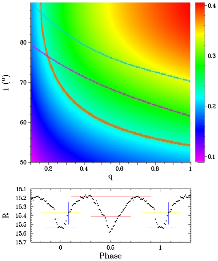
Figure 5: Bottom: Mean phase folded light curve of GY Hya observed in 2004. The magnitudes levels of the orbital maxima and of ingress and egress of the secondary eclipse are marked by red horizontal lines. Their difference $\delta m$ is a lower limit to the ellipsoidal variation of the secondary star. Similarly, the difference between the yellow horizontal lines defines an upper limit to the primary eclipse depth $\Delta m_{\rm ecl}$. The blue vertical lines indicate the outer contact phase of the primary eclipse. Top: The total amplitude $\Delta m$ of ellipsoidal variations (the colour code is specified on the colour bar at the right) of the secondary star in GY Hya as a function of the assumed mass ratio $q$ and orbital inclination $i$. The brown solid curve separates permitted $q-i$ combinations ($\Delta m>\delta m$) to the upper right from forbidden combinations ($\Delta m<\delta m$) to the lower left. The light blue and violet solid lines represent the functional relationship between $q$ and $i$ derived from the observed outer eclipse contact phase and Roche geometry for assumed disk radii of $0.2A$ and $0.3A$, respectively, where $A$ is the distance between the primary and secondary components. (For interpretation of the references to colour in this figure legend, the reader is referred to the web version of this article.)

Assuming the radius $R_{\rm d}$ of the accretion disk (taken to be flat and infinitesimally thin) to be known, Roche geometry and the last contact phase of the disk eclipse provide a functional relationship between $q$ and $i$. The last contact is quite well defined in the light curve. It occurs at phase 0.074 (blue vertical lines in Fig. 5, lower frame). In quiescent dwarf novae $R_{\rm d}\approx 0.3$ [in units of the component separation; e.g. OY Car: 0.31 (Wood et al. 1989); Z Cha: 0.33 (Wood et al. 1986); V2051 Oph: 0.32 (Baptista et al. 2007); V4104 Sgr: 0.28 (Borges & Baptista 2005)]. Adopting this value we numerically derived the $q-i$ relationship which is shown as a violet line in the upper frame of the figure.

For all values of $q>0.3$, the observed outer contact phase together with $R_{\rm d}=0.3$ leads to a configuration such that the central parts of the disk remain uneclipsed. For $q\rightarrow 1$ only a small part of the outer disk is invisible at mid-eclipse. This is hardly compatible with the observed eclipse depth. Moreover, the eclipse depth during outburst (Sect. 3.3) should then not reach the same low level seen in quiescence because the central parts of the then bright accretion disk would remain visible. Therefore, in order to assess the effect of a smaller disk radius, we also calculated the $q-i$ relation for $R_{\rm d}=0.2$ which is shown as a light blue line in the figure. We remark that for this disk radius the centre of the primary is eclipsed for all $q$ and the disk eclipse is total for $q<0.75$.

The strong ellipsoidal variations attest to the dominant contribution of the secondary star to the total light. An upper limit to the relative contribution of the primary component ($I_{1}$, expressed in units of the secondary contribution $I_{2}$ at orbital maximum) can be calculated as a function of the intrinsic amplitude of the ellipsoidal variations ($\Delta m$) from their observed amplitude ($\delta m$). For $\Delta m$ between the maximum value in Fig. 5 and a value just above its permitted minimum value $\delta m$ the contribution of the primary must remain below the back line in Fig. 6 (left hand scale).

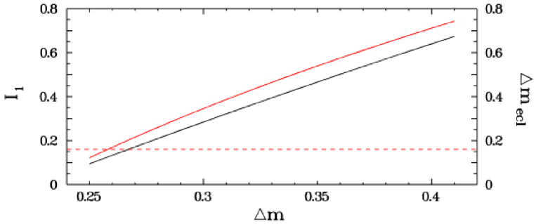
Figure 6: Upper limit to the relative contribution $I_{1}$ of the primary star light of GY Hya (in units of the secondary star light at orbital maximum) as a function of the intrinsic amplitude $\Delta m$ of the ellipsoidal variations of the secondary (black line, left hand scale). Upper limit of the primary eclipse depth $\Delta m_{\rm ecl}$ (total eclipse assumed) as a function of $\Delta m$ (red line, right hand scale). The broken line indicates the observed eclipse depth. (For interpretation of the references to colour in this figure legend, the reader is referred to the web version of this article.)

Is this compatible with the observed primary eclipse depth $\Delta m_{\rm ecl}$? Yes, it is. Assuming the eclipse to be total, an upper limit for $\Delta m_{\rm ecl}$ can be calculated from $I_{2}$, $\Delta m$ and the upper limit to $I_{1}$. This is shown as a red line in Fig. 6 (right hand scale). The observed primary eclipse depth can be estimated from the magnitude difference at mid-eclipse and the end of eclipse egress in the lower frame of Fig. 5 to be not more than $\Delta m_{\rm ecl}=0^{\raisebox{0.90417pt}{\scriptsize m}}_{\raisebox{1.80835pt}{\hskip 1.18999pt.}}16$ (difference between the yellow horizontal lines). This is an upper limit because due to its ellipsoidal variations the secondary contributes less at mid-eclipse than at the end of egress. $\Delta m_{\rm ecl}$ is shown as a broken line in Fig. 6. Obviously, the observed eclipse depth is significantly smaller than than the calculated upper limit for all but the smallest values of $\Delta m$.

While the above considerations lead to a consistent picture of GY Hya a problem arises when regarding some low points which appear in the long term light curve (Fig. 1). Even for the maximum upper limit of $I_{1}$ (referring to the maximum of value of $\Delta m$ considered here) the brightness of the system cannot decrease by more than $\sim$$0^{\raisebox{0.90417pt}{\scriptsize m}}_{\raisebox{1.80835pt}{\hskip 1.18999pt.}}56$ even under the extreme assumption that the primary star contribution drops to zero. How can GY Hya then attain a magnitude as faint as $16^{\raisebox{0.90417pt}{\scriptsize m}}_{\raisebox{1.80835pt}{\hskip 1.18999pt.}}9$? Most of the low points are concentrated in a small time interval between 2001, April 27 and June 27 and were observed by the same observer (who did not contribute any other data). Moreover, at least on two occasions other observers found the system to be at a “normal” magnitude just two days before or after a faint observation. The one remaining low point at JD 2452842 is the only data point provided by another observer. This may cast doubts on the reliability of the faint data points.

5 Summary

We present the first time resolved photometry of the CV GY Hya. Its overall behaviour is as expected from a dwarf nova with a long orbital period. The light curve is characterized by strong orbital modulations in quiescence caused by ellipsoidal variations of the dominant mass donor star together with eclipses of both system components. As is normal in cataclysmic variables, flickering is present but on a magnitude scale significantly smaller than in most quiescent dwarf novae (Beckemper 1995) because the flickering light source, expected to be associated to the accretion disk, is outshone by the brighter secondary star. The average light curves show some variability in different observing seasons which can qualitatively be explained by a variable contribution of a hot spot to the total light together with changes of the disk radius. There are some indications that the disk radius, expressed in units of the component separation, is smaller than observed in other dwarf novae.

References

Allen, C.W. 1973, Astrophysical Quantities, third edition (Athlone Press: London)

Baptista, R., Santos, R.F., Faúndez-Abans, M., & Bortoletto, A. 2007, AJ, 134, 867

Beckemper, S. 1995, Statistische Untersuchungen zur Stärke des Flickering in kataklysmischen Veränderlichen, Diploma thesis, Münster

Bond, H.E., & Tifft, W.G. 1974, PASP, 86, 981

Borges, B., & Baptista, R. 2005, A&A 437, 325

Bruch, A. 1993, MIRA: A Reference Guide (Astron. Inst. Univ. Münster)

Bruch, A. 2016, New Astr., 46, 90

Bruch, A. 2017, New Astr., 52, 112

Bruch, A., & Diaz, M.P. 2017, New Astr., 50, 109

Claret, A., & Bloemen, S. 2011, A&A, 529, A75

Cropper, M. 1986, MNRAS 222, 225

Eastman, J., Siverd, R., & Gaudi, B.S. 2010, PASP, 122, 935

Hoffmeister, C. 1963, Veröff. Sternw. Sonneberg, 6, 38

Peters, C.S., & Thorstensen, R. 2005, PASP 117, 1386

Williams, G. 1983, ApJ Suppl., 53, 523

Wilson, R.E. 1979, ApJ, 234, 1054

Wilson, R.E., & Devinney, E.J. 1971, ApJ, 166, 605

Wood, J.A., Horne, K., & Berriman G. 1989, ApJ, 341, 974

Wood, J.A., Horne, K., Berriman G., et al. 1986, MNRAS, 219, 629

Zacharias, N., Finch, C.T., Girard, T.M., et al. 2013, AJ, 145, 44

Zwitter, T., & Munari, U. 1996, A&AS, 117, 449