One-dimensional granular system with memory effects

Abstract

We consider a hybrid compressible/incompressible system with memory effects, introduced recently by Lefebvre Lepot and Maury for the description of one-dimensional granular flows. We prove a global existence result for this system without assuming additional viscous dissipation. Our approach extends the one by Cavalletti et al. for the pressureless Euler system to the constrained granular case with memory effects. We construct Lagrangian solutions based on an explicit formula using the monotone rearrangement associated to the density. We explain how the memory effects are linked to the external constraints imposed on the flow. This result can also be extended to a heterogeneous maximal density constraint depending on time and space.

Keywords: Granular flows, pressureless gas dynamics.

MSC: 35Q35, 49J40, 76T25.

Introduction

In this paper, we consider a one-dimensional model for immersed granular flows, introduced by Lefebvre-Lepot and Maury in [16] and [17]. The model consists of a system of nonlinear partial differential equations describing the solid/liquid mixture through the evolution of the density of solid particles $\rho$ and the Eulerian velocity field $u$. It takes the form

$$\partial_{t}\rho+\partial_{x}(\rho u)=0$$ (1a)

$$\partial_{t}(\rho u)+\partial_{x}(\rho u^{2})+\partial_{x}p=\rho f$$ (1b)

$$\partial_{t}\gamma+u\partial_{x}\gamma=-p$$ (1c)

$$0\leq\rho\leq 1$$ (1d)

$$(1-\rho)\gamma=0,\quad\gamma\leq 0,$$ (1e)

where $p$ represents the pressure, and $f$ is an external force. Equations (1a) and (1b) express the local conservation of mass and momentum, respectively. The density is confined to values between $0$ (vacuum) and $1$ (for simplicity of presentation), with $\rho=1$ representing the congested state. The pressure $p$ plays the role of Lagrange multiplier for this pointwise constraint: through the momentum equation (1b), it acts on the fluid to ensure that condition (1d) remains satisfied everywhere. The amount of compression that the fluid is exposed to, but cannot accommodate because of (1d), is captured in the adhesion potential $\gamma$, which is linked to the pressure $p$ through Equation (1c). It expresses a memory effect, keeping track of the history of the constraint satisfaction of the system over the course of time.

The system of Equations (1a)–(1e) therefore model two very different regimes that occur in the flow: in free zones, characterized by the condition $\rho<1$, we have a pressureless dynamics of a compressible flow. In this regime, both $p$ and $\gamma$ vanish; see (1e) and (1c). In the congested zones, characterized by $\rho=1$, we have the dynamics of an incompressible flow. The continuity equation (1a) implies that in congested zones the velocity must satisfy $\partial_{x}u=0$ so that the action of the external force $f$ must be balanced by the pressure $p$, which in turn is recorded into the adhesion potential $\gamma$. Note that in [16, 17] instead of (1c) the equation

$$\partial_{t}\gamma+\partial_{x}(\gamma u)=-p$$ (2)

is considered, which is formally equivalent to (1c) since $\partial_{x}u=0$ if $\rho=1$. On the other hand, if $\rho<1$, then $\gamma$ must vanish because of (1e). We would argue, however, that the form (1c) is more natural. In fact, differentiating this equation with respect to $x$, we obtain

$$\partial_{t}\big{(}\partial_{x}\gamma\big{)}+\partial_{x}\big{(}u\partial_{x}\gamma\big{)}=-\partial_{x}p.$$ (3)

Subtracting this equation from (1b), we observe that the pressure term cancels, giving

$$\partial_{t}(\rho u-\partial_{x}\gamma)+\partial_{x}\big{(}(\rho u-\partial_{x}\gamma)u\big{)}=\rho f.$$ (4)

Hence $\partial_{x}\gamma$ plays the role of an additional momentum. Because of the exclusion relation (1e), the adhesion potential $\gamma$ can only be different from zero where $\rho=1$, thus $\partial_{x}\gamma$ is absolutely continuous with respect to $\rho$. In principle, it is therefore possible to define a velocity $v$ such that $\partial_{x}\gamma=\rho v$. We can then rewrite (4) with $w:=u-v$ in the form

$$\partial_{t}(\rho w)+\partial_{x}(\rho uw)=\rho f.$$ (5)

In [17], the system (1e) has been supplemented with a collision law that prevents elastic shocks between congested blocks. This condition can be expressed as

$$u(t^{+})=\mathrm{P}_{\mathrm{Adm}_{\rho,\gamma}}\big{(}u(t^{-})\big{)},$$ (6)

where $u(t^{\pm})$ denotes the one-sided limits of the velocity at time $t$, and with $\mathrm{P}_{\mathrm{Adm}_{\rho,\gamma}}$ the $L^{2}$ projection onto the set of admissible velocities, defined as the $L^{2}$ closure of

$$\left\{v\in H^{1}\colon\begin{cases}\partial_{x}v\geq 0~{}\text{a.e. on}~{}\{\rho=1,\gamma=0\}\\ \partial_{x}v=0~{}\text{a.e. on}~{}\{\rho=1,\gamma<0\}\end{cases}\right\}.$$

The memory effects exhibited by system (1e) have been brought to light by Maury [17] in the case of a single solid particle. He examined a physical system formed by a vertical wall and a spherical solid particle that is immersed in a viscous liquid. The particle evolves along the horizontal axis and is submitted to an external force and to the lubrication force exerted by the liquid. The latter becomes predominant when the particle is getting closer to the wall. At first order when the distance $q$ between the particle and the wall goes to $0$, it takes the form $F_{\text{lub}}=-C\eta\,\frac{\dot{q}}{q}$, with $\eta$ the viscosity of the liquid, $C>0$ a constant that depends on the diameter of the particle. It prevents the contact in finite time of particle and wall.

Considering the limit of vanishing liquid viscosity $\eta=\varepsilon\rightarrow 0$, Maury proved in [17] the convergence toward a hybrid system (see system (19b) below) describing the two possible states of the system: free when $q>0$ and stuck when $q=0$. In the limit, the system involves a new variable $\gamma$, the adhesion potential, which is the residual effect of the singular lubrication force $F^{\varepsilon}_{\text{lub}}$ for $\varepsilon\rightarrow 0$. The potential describes the stickyness of the particle: even in case of a pulling external force, it may take some time before the particle takes off from the wall.

Lefebvre-Lepot and Maury have extended this idea to a one-dimensional macroscopic system of aligned solid particles: system (1e) is obtained in [16] as the formal limit of

$$\partial_{t}\rho_{\varepsilon}+\partial_{x}(\rho_{\varepsilon}u_{\varepsilon})=0$$ (7a)

$$\partial_{t}(\rho_{\varepsilon}u_{\varepsilon})+\partial_{x}(\rho u_{\varepsilon}^{2})-\partial_{x}\left(\dfrac{\varepsilon}{1-\rho_{\varepsilon}}\partial_{x}u_{\varepsilon}\right)=\rho_{\varepsilon}f.$$ (7b)

The lubrication force is represented at this macroscopic scale by the singular viscous term $\partial_{x}(\frac{\varepsilon}{1-\rho_{\varepsilon}}\partial_{x}u_{\varepsilon})$, which prevents, by analogy with the single particle case, the formation of congested domains $\rho=1$ when $\varepsilon>0$. The rigorous proof, however, of the convergence of solutions of (7b) to solutions of (1e) remains an open problem. The mathematical difficulty of this singular limit relies in the lack of compactness of the non-linear term $\rho_{\varepsilon}u_{\varepsilon}^{2}$. This kind of singular limit has nevertheless been proved in [20] (see also [21] for a result in dimension 2) on an augmented system where an additional physical dissipation is taken into account.

In this paper, we want to study the system (1e) directly, without any lubrication approximation. For that purpose, we take advantage of the link between model (1e) and the model of pressureless gas dynamics in one space dimension:

$$\partial_{t}\rho+\partial_{x}(\rho u)=0$$ (8a)

$$\partial_{t}(\rho u)+\partial_{x}(\rho u^{2})=0.$$ (8b)

We establish a global existence result for weak solutions to the following system:

$$\partial_{t}\rho+\partial_{x}(\rho u)=0$$ (9a)

$$\partial_{t}(\rho u-\partial_{x}\gamma)+\partial_{x}\big{(}(\rho u-\partial_{x}\gamma)u\big{)}=\rho f$$ (9b)

$$0\leq\rho\leq 1$$ (9c)

$$(1-\rho)\gamma=0,\quad\gamma\leq 0.$$ (9d)

Among the large literature that exists for the pressureless system (8b), we are interested in the recent results of Natile and Savaré [19] and Cavalletti et al. [10] that develop a Lagrangian approach based on the representation of the density $\rho$ by its monotone rearrangement $X$, which is the optimal transport between the Lebesgue measure $\mathcal{L}^{1}_{|[0,1]}$ and $\rho$; see [25].

Let us also mention that the granular system (1e) can be seen as a non-trivial extension of the pressureless Euler equations under maximal density constraint

$$\partial_{t}\rho+\partial_{x}(\rho u)=0$$ (10a)

$$\partial_{t}(\rho u)+\partial_{x}(\rho u^{2})+\partial_{x}\pi=0$$ (10b)

$$0\leq\rho\leq 1$$ (10c)

$$(1-\rho)\pi=0,\quad\pi\geq 0.$$ (10d)

This system has been first introduced by Bouchut et al. [6] as a model of two-phase flows and then studied by Berthelin [4] and Wolansky [27]. The results rely on a discrete approximation generalizing the sticky particle dynamics used for the pressureless system. Recently, numerical methods based on optimal transport tools have been developed for this system; see [18, 23].

For viscous fluids, i.e., Navier-Stokes systems, a theoretical existence result can be found in [22] in the case where the maximal density constraint $\rho^{*}(x)$ is a given function of the space variable. Recently, Degond et al. have proved in [11] the existence of global weak solutions to the Navier-Stokes system with a time and space dependent maximal constraint $\rho^{*}(t,x)$ that is transported by the velocity $u$: it satisfies the transport equation

$$\partial_{t}\rho^{*}+u\,\partial_{x}\rho^{*}=0.$$ (11)

Numerical simulations are have been studied in [11, 12] with applications to crowd dynamics. This type of heterogeneous maximal constraint may be also relevant for the dynamics of floating structures; see for instance Lannes [14].

The paper is organized as follows:

In Section 1 we briefly review the literature on the pressureless gas dynamics and introduce the mathematical tools linked to a Lagrangian description. In Section 2 we explain formally how these tools can be extended to the system (9d) and give our main existence result. Section 3 is devoted to the proof of this result and Section 4 presents some numerical simulations. In the last section, we extend finally the result to the special case of time and space dependent maximal density constraint that satisfies the transport equation (11).

1 Lagrangian approach for the pressureless Euler equations

The pressureless gas dynamics equations, augmented by the assumption of adhesion dynamics, has been proposed as a simple model for the formation of large scale structures in the universe such as aggregates of galaxies. It is linked to the sticky particle system introduced by Zeldovich in [28]. The work of Bouchut [5] highlights the obstacles to proving existence of classical solutions to (8b) (concentration phenomena on the density, lack of uniqueness under classical entropy conditions). Since then, several different mathematical approaches have been proposed in the literature for proving the global existence of measure solutions under suitable entropy conditions (see again [5]), among which there are approximations by the discrete sticky particles dynamics [9, 19], approximation by viscous regularization [26, 7] or, more recently, derivation by a hydrodynamic limit [13].

In particular, Natile and Savaré use [19] an interesting Lagrangian characterization of the density $\rho$ by its monotone rearrangement $X$ to show convergence of the discrete sticky particle system as the number $N$ of particles goes to $+\infty$. To every probability measure $\rho\in\mathcal{P}_{2}(\mathbb{R})$ (i.e., with finite quadratic moment $\int_{\mathbb{R}}|x|^{2}\,\rho(dx)<+\infty$) there is associated a unique transport $X\in K$, the closed convex cone of non-decreasing maps in $L^{2}(0,1)$, such that

$$\rho_{t}=(X_{t})_{\#}\mathcal{L}^{1}_{|[0,1]}.$$ (12)

Here $\mathcal{L}^{1}_{|[0,1]}$ is the one-dimensional Lebesgue measure restricted to the interval $[0,1]$ and $\#$ denotes the push-forward of measures, defined for all Borel maps $\zeta\,:\,\mathbb{R}\rightarrow[0,\infty]$ by

$$\int_{\mathbb{R}}\zeta(x)\,\rho_{t}(dx)=\int_{0}^{1}\zeta\big{(}X_{t}(y)\big{)}\,dy.$$ (13)

If now $(\rho,u)$ is a solution in the distributional sense of (8b), then $u_{t}$ can be associated to the Lagrangian velocity $U_{t}:=\dot{X}_{t}$ (in the sequel all the Lagrangian variables will be denoted by capital letters and the Eulerian ones by the corresponding small letters) through

$$U_{t}(y)=u_{t}\big{(}X_{t}(y)\big{)}.$$ (14)

In [19], Natile and Savaré show different characterizations of the transport $X$ associated to an Eulerian solution of (8b), in particular they prove that

$$X_{t}=\mathrm{P}_{K}\big{(}\bar{X}+t\bar{U}\big{)}\quad\text{for all $t\geq 0$,}$$ (15)

where $\mathrm{P}_{K}$ is the $L^{2}(0,1)$ projection onto the closed convex set $K$ and $\bar{X},\bar{U}$ are respectively the monotone rearrangement and the Lagrangian velocity associated to the initial data. The map $\bar{X}+t\bar{U}$ represents the free motion path, which is at the discrete level the transport corresponding to the case where the particles do not interact at all.

These arguments have been extended by Brenier et al. [8] to systems including an interaction between the discrete particles. This interaction is represented at the continuous level by a force $f(\rho)$ in the right-hand side of the momentum equation (8b).

Recently, Cavalletti et al. [10] have taken advantage of the formula (15) to construct directly global weak solutions to (8b) without any discrete approximation by sticky particles. To this end, they define for all positive times $t$ the transport $X_{t}$, associated to an initial data $(\bar{\rho},\bar{u})$, by equation (15). The Lagrangian variables $\bar{X}$ and $\bar{U}$ are defined by

$$\bar{\rho}=(\bar{X})_{\#}\mu,\quad\bar{U}:=\bar{u}\circ\bar{X}$$ (16)

for a more general reference measure $\mu$ in $\mathcal{P}_{2}(\mathbb{R})$ (for instance $\mu=\bar{\rho}$ and in this case $\bar{X}=\mathrm{id}$). As a consequence of the contraction property of the projection operator $\mathrm{P}_{K}$, the map $t\mapsto X_{t}$ is Lipschitz continuous and thus differentiable for a.e. $t$, which allows us to define the Lagrangian velocity $U_{t}:=\dot{X}_{t}$. Cavalletti et al. [10] introduce the subspace in $L^{2}(\mathbb{R},\mu)$ formed by functions which are essentially constant where $X_{t}$ is constant:

$$\mathcal{H}_{X_{t}}=\text{$L^{2}(\mathbb{R},\mu)$-closure of}~{}\big{\{}\varphi\circ X_{t}\colon\varphi\in\mathcal{D}(\mathbb{R})\big{\}}.$$ (17)

This space is a subset of the tangent cone to $K$ at $X_{t}$, denoted by $\mathbb{T}_{X_{t}}K$, in which the Lagrangian velocity is contained. One can then show that $U_{t}$ is the orthogonal projection of $\bar{U}$ onto the space $\mathcal{H}_{X_{t}}$:

$$U_{t}=\mathrm{P}_{\mathcal{H}_{X_{t}}}(\bar{U}).$$ (18)

This property ensures that there exists, for a.e. $t$, an Eulerian velocity $u_{t}\in L^{2}(\mathbb{R},\rho_{t})$ with the property that $U_{t}=u_{t}\circ X_{t}$. This is the key argument for recovering the weak formulations of the gas dynamics equations (8a)–(8b) in the Eulerian formulation.

By comparison, our granular system written under the pressureless form (9d) involves an additional maximal density constraint $\rho\leq 1$, an additional variable $\gamma$ linked to this maximal constraint, and an external force $f$. We explain in the next section how to extend the previous tools in order to deal with these additional constraints and variables.

2 Extension to granular flows, main result

Before announcing our existence result, we need to explain how to adapt the Lagrangian tools mentioned above when an external force and a maximal density constraint is given. A good way to do this is to come back to the microscopic approach, by nature Lagrangian, developed by Maury in [17] for a single sticky particle in contact with a wall.

Single particle case.

Maury [17] proves by a vanishing viscosity limit (viscosity of liquid in which the particle is immersed), the existence of solutions to the hybrid system

$$\dot{q}+\gamma=\bar{u}+\int_{0}^{t}{f(s)\,ds}$$ (19a)

$$q\geq 0,\quad\gamma\leq 0,\quad q\,\gamma=0,$$ (19b)

which describes the two possible states of the system: free when $q>0$ (that is, the particle evolves freely under the external force $f$), and stuck whenever $q=0$. In this latter case, the adhesion potential is activated and is equal to

$$u^{\text{free}}(t)=\bar{u}+\int_{0}^{t}{f(s)\,ds},$$ (20)

which is the velocity the particle would have if there was no wall on its trajectory. System (19b) is in fact equivalent to the following second order system (see [15])

$$\ddot{q}=f+\lambda$$ (21a)

$$\dot{q}(t^{+})=\mathrm{P}_{C_{q,\gamma}(t)}\dot{q}(t^{-})$$ (21b)

$$\mathrm{spt}\,(\lambda)\subset\{t\colon q(t)=0\}$$ (21c)

$$\dot{\gamma}=-\lambda$$ (21d)

$$q\geq 0,\quad\gamma\leq 0,$$ (21e)

where $C_{q,\gamma}(t)$ denotes the set of admissible velocities

$$C_{q,\gamma}(t)=\begin{cases}~{}\{0\}\quad&\text{if}\quad\gamma(t^{-})<0\\ ~{}\mathbb{R}^{+}\quad&\text{if}\quad\gamma(t^{-})=0,~{}q(t)=0\\ ~{}\mathbb{R}\quad&\text{otherwise.}\end{cases}$$

It ensures that the particle cannot cross the wall and that it sticks to the wall as long as $\gamma<0$. By comparison with system (1e), an analogy can be made between the variables $q$ and $1-\rho$, between $\lambda$ and $-\partial_{x}p$ and thus between $\gamma_{\text{micro}}$ defined by (21d) and $-\partial_{x}\gamma_{\text{macro}}$.

Extension of the Lagrangian approach.

Let $\rho_{0}\in\mathcal{P}_{2}(\mathbb{R})$ denote the initial density. We assume that $\rho_{0}$ is absolutely continuous with respect to the Lebesgue measure and that its density (also denoted $\rho_{0}$, for simplicity) satisfies the maximal constraint

$$0\leq\rho_{0}\leq 1\quad\text{a.e.}$$ (22)

As suggested by Cavalletti et al. [10] we set $\bar{\rho}=\rho_{0}$ as reference measure.

Definition 2.1.

The set of square-integrable functions with respect to the measure $\bar{\rho}$ will be denoted $L^{2}(\mathbb{R},\bar{\rho})$. Let $\langle\cdot,\cdot\rangle$ be the induced inner product. The space of $p$-integrable functions on the domain $\Omega$ for the Lebesgue measure will be denoted by $L^{p}(\Omega)$.

In the following, we will switch freely between absolutely continuous measures $\rho(dx)$ and their Lebesgue densities $\rho(x)\,dx$. The meaning will be clear from the context.

Set of admissible transports. To each $\rho_{t}$ we associate a monotone transport map $X_{t}$ through

$$\rho_{t}=(X_{t})_{\#}\bar{\rho}.$$ (23)

To express the maximal density constraint $\rho_{t}\leq 1$ in terms of a constraint on the transport map $X_{t}$, we consider a maximally compressed density with the same total mass as $\bar{\rho}$, which is a characteristic function of some interval $\widetilde{I}$ of length one. For definiteness, we assume this interval to be centered around the center of mass of $\bar{\rho}$, but the construction is invariant under translation since constants can be absorbed into the transport map. Let $\widetilde{\rho}$ be the probability measure associated to the characteristic function of $I_{0}$. Let $\widetilde{X}$ be the unique nondecreasing transport map in $L^{2}(\mathbb{R},\bar{\rho})$ (see [25] Theorem 2.5, for example) such that

$$\widetilde{\rho}=\widetilde{X}_{\#}\bar{\rho}.$$ (24)

The push forward formula implies that $\partial_{y}\widetilde{X}(y)>0$ for $\bar{\rho}$-a.e. $y\in\mathbb{R}$ and

$$\widetilde{\rho}(x)=\frac{\bar{\rho}(\widetilde{X}^{-1}(x))}{\partial_{y}\widetilde{X}(\widetilde{X}^{-1}(x))}\quad\text{for a.e. $x\in I_{0}$;}$$ (25)

see [2] Lemma 5.5.3. In particular, we have $\bar{\rho}(y)/\partial_{y}\widetilde{X}(y)=1$ for $\bar{\rho}$-a.e. $y\in\mathbb{R}$. The measure $\rho_{t}$ in (23) is absolutely continuous with respect to the Lebesgue measure if and only if the approximate derivative $\partial_{y}X_{t}(y)>0$ for $\bar{\rho}$-a.e. $y\in\mathbb{R}$. For $\rho_{t}$-a.e. $x\in\mathbb{R}$, we then have

$$\rho_{t}(x)=\dfrac{\bar{\rho}(X_{t}^{-1}(x))}{\partial_{y}X_{t}(X_{t}^{-1}(x))}=\dfrac{\bar{\rho}(X_{t}^{-1}(x))}{\partial_{y}\widetilde{X}(X_{t}^{-1}(x))}\,\dfrac{\partial_{y}\widetilde{X}(X_{t}^{-1}(x))}{\partial_{y}X_{t}(X_{t}^{-1}(x))}=\dfrac{\partial_{y}\widetilde{X}(X_{t}^{-1}(x))}{\partial_{y}X_{t}(X_{t}^{-1}(x))}.$$ (26)

In order to guarantee the maximal density constraint we are thus led to consider transport maps $X_{t}$ such that $\partial_{y}\widetilde{X}(y)\leq\partial_{y}X_{t}(y)$ for $\bar{\rho}$-a.e. $y\in\mathbb{R}$. We therefore introduce the closed convex set of admissible transports maps in $L^{2}(\mathbb{R},\bar{\rho})$ as follows: We define

$$\widetilde{K}:=K+\widetilde{X},$$ (27)

where $K$ is the cone of monotone (more precisely: non-decreasing) maps of $L^{2}(\mathbb{R},\bar{\rho})$. To the transport map $X_{t}\in\widetilde{K}$, we associate the monotone transport map

$$S_{t}:=X_{t}-\widetilde{X}\in K.$$ (28)

Note that monotone maps are differentiable a.e., with nonnegative derivative.

Remark 2.2.

Coming back to the definition of $\widetilde{\rho}$, we observe that the position of the interval $\widetilde{I}$ does not matter for the definition of $\widetilde{K}$ since the translations can be absorbed in $K$.

Formal description of the dynamics. In order to define for all times $t$ an appropriate transport map $X_{t}$, we need to extend the notion of free transport $\bar{X}+t\bar{U}$ used in (15) to the case where the external force $f$ is applied on the system. In particular, we need to extend the notion of free velocity, which for the pressureless system is simply the initial velocity $\bar{U}$. In our case, inspired by the microscopic case (20), we are naturally led to set

$$U^{\text{free}}_{t}:=\bar{U}+\int_{0}^{t}{f(s,X_{s})\,ds},$$ (29)

integrating along the trajectories $t\mapsto X_{t}(y)$ starting at $y$. The free trajectory at time $t$ would be then be given by the formula

$$X^{\text{free}}_{t}:=\bar{X}+\int_{0}^{t}{U^{\text{free}}_{s}\,ds},$$ (30)

and in analogy with (15), we consider

$$X_{t}:=\mathrm{P}_{\widetilde{K}}(X^{\text{free}}_{t})=\mathrm{P}_{\widetilde{K}}\left(\bar{X}+\int_{0}^{t}{U^{\text{free}}_{s}\,ds}\right);$$ (31)

see [8] for a similar formulation. Note carefully that equations (31)–(29) form a coupled system insofar as the free velocity $U^{\text{free}}_{t}$ depends on the trajectory $X_{s}$ itself. Establishing the existence and uniqueness of a solutions is non trivial and requires suitable assumptions on the external force $f$. We detail this point in Lemma 3.1 below. The associated velocity, formally defined as $U_{t}=\frac{d}{dt}X_{t}$, not only has to belong the tangent cone to $K$ at $S_{t}=X_{t}-\widetilde{X}$, defined as

$$\mathbb{T}_{S_{t}}K:=\text{$L^{2}(\mathbb{R},\bar{\rho})$-closure of $T_{S_{t}}K$}\quad\text{where}\quad T_{S_{t}}K:=\bigcup_{h>0}h\big{(}K-S_{t}\big{)},$$ (32)

it has to be constant on each congested block for a.e. $t$. That is, $U_{t}$ must belong to the set

$$\mathcal{H}_{S_{t}}:=\left\{U\in L^{2}(\mathbb{R},\bar{\rho})\colon\text{$U$ is a.e. constant on maximal intervals in $\Omega_{S_{t}}$}\right\}$$ (33)

where $\Omega_{S_{t}}$ is the union of all non-trivial intervals on which $S_{t}$ is constant. In analogy to the microscopic case (19a), we define an adhesion potential $\Gamma_{t}$; see (39).

Definition of weak solutions and main result.

Here is our solution concept.

Definition 2.3.

Given suitable initial data $(\bar{\rho},\bar{u})$, a triple $(\rho,u,\gamma)$ is called a weak solution of system (9d) provided that

• $(\rho,u,\gamma)$ satisfies

  $$\rho_{t}\in\mathcal{P}_{2}(\mathbb{R}),\;u_{t}\in L^{2}(\mathbb{R},\rho_{t})\quad\text{for a.e. $t\in[0,T]$},$$ (34)

  $$\gamma\in L^{\infty}\big{(}[0,T];W^{1,1}(\mathbb{R})\big{)};$$ (35)

• the density constraint (9c) and the exlusion principle (9d) hold almost everywhere;

• equations (9a) and (9b) are satisfied in the sense of distributions:

  $$\int_{0}^{T}\int_{\mathbb{R}}\Big{(}\partial_{t}\xi(t,x)+u_{t}(x)\partial_{x}\xi(t,x)\Big{)}\rho_{t}(x)\,dx\,dt$$ (36)

  $$\qquad\qquad=-\int_{\mathbb{R}}{\xi(0,x)\,\bar{\rho}(x)\,dx}\quad\text{for all $\xi\in\mathcal{C}^{\infty}_{c}\big{(}[0,T)\times\mathbb{R}\big{)}$,}$$

  $$\int_{0}^{T}\int_{\mathbb{R}}\Big{(}\partial_{t}\varphi(t,x)+u_{t}(x)\partial_{x}\varphi(t,x)\Big{)}\big{(}\rho_{t}(x)u_{t}(x)-\partial_{x}\gamma_{t}(x)\big{)}\,dx\,dt$$ (37)

  $$\qquad\qquad+\int_{0}^{T}\int_{\mathbb{R}}\varphi(t,x)\,\rho_{t}(x)f_{t}(x)\,dx\,dt$$

  $$\qquad\qquad=-\int_{\mathbb{R}}\varphi(0,x)\,\bar{\rho}(x)\bar{u}(x)\,dx\quad\text{for all $\varphi\in\mathcal{C}^{\infty}_{c}\big{(}[0,T)\times\mathbb{R}\big{)}$.}$$

Remark 2.4.

As explained before, the velocity must be compatible with the flow configuration in the sense that it is non-decreasing on congested blocks; recall (33). We can write

$$\bar{\rho}(x)\bar{u}(x)=\bar{\rho}(x)u_{0}(x)-\partial_{x}\gamma_{0}(x),$$

where $u_{0}$ is the $L^{2}(\mathbb{R},\bar{\rho})$-projection of $\bar{u}$ onto the tangent cone $\mathbb{T}_{S_{0}}K$ and the adhesion potential $\gamma_{0}$ is defined in analogy to (39).

Theorem 2.5.

Let $T>0$ and external force $f\in L^{\infty}\big{(}0,T;\mathrm{Lip}(\mathbb{R})\cap L^{\infty}(\mathbb{R})\big{)}$ be given. Suppose that $\bar{\rho}\in\mathcal{P}_{2}(\mathbb{R})$ with $\bar{\rho}\ll\mathcal{L}^{1}$ and $0\leq\bar{\rho}\leq 1$ a.e., and that $\bar{u}\in L^{2}(\mathbb{R},\bar{\rho})$. Define

$$\bar{X}:=\mathrm{id},\;\bar{U}:=\bar{u},\quad\text{so that}\quad X_{0}=X_{0}^{\text{free}}=\mathrm{id},\;U^{\text{free}}_{0}=\bar{u},\;\rho_{0}:=\bar{\rho}.$$ (38)

There exists a curve $[0,T]\ni t\mapsto X_{t}\in\widetilde{K}$ that is differentiable for a.e. $t\in(0,T)$ and solves the coupled system of equations (29)–(31). The following quantities are well-defined:

$$U_{t}(y):=\dot{X}_{t}(y),\;\Gamma_{t}(y):=\int_{-\infty}^{y}{\Big{(}U_{t}(z)-U^{\text{free}}_{t}(z)\Big{)}\bar{\rho}(z)\,dz}$$ (39)

for $y\in\mathbb{R}$ and a.e. $t\in(0,T)$. There exist $(u_{t},\gamma_{t})\in\mathcal{L}^{2}(\mathbb{R},\rho_{t})\times W^{1,1}(\mathbb{R})$, such that

$$U_{t}=u_{t}\circ X_{t},\;\Gamma_{t}=\gamma_{t}\circ X_{t}\quad\text{where}\quad\rho_{t}:=(X_{t})_{\#}\bar{\rho}.$$

The triple $(\rho,u,\gamma)$ is a global weak solution of system (9d).

Remark 2.6.

The assumption $f\in L^{\infty}\big{(}0,T;\mathrm{Lip}(\mathbb{R})\cap L^{\infty}(\mathbb{R})\big{)}$ can be relaxed to include a larger class of forces. We will stick to it here to simplify the presentation.

Notice that $X_{0}=\mathrm{id}$ satisfies (26) for $t=0$, hence $X_{0}\in\widetilde{K}$ as expected.

3 Construction of global weak solutions

Our proof consists of three steps. First we establish existence and uniqueness of $X_{t}$ (defined by (31)) and $U_{t}$. We will prove that the velocity $U_{t}$ is admissible in the sense that it belongs to the set $\mathcal{H}_{S_{t}}$ defined in (33). Introducing next the adhesion potential as in (39), we show in Subsection 3.2 that it is non-positive and supported in the congested domain. Finally, we check in Subsection 3.3 that the Eulerian variables $(\rho,u,\gamma)$ associated to $(X_{t},U_{t},\Gamma_{t})$ with $t\in[0,T]$ satisfy the weak formulations (36)–(37) of system (9d).

3.1 Definition of the transport and velocity

Let us begin by justifying the fact that we can define in a unique manner $X_{t}$ for all times.

Lemma 3.1.

For all $t\in[0,T]$, there exists a unique solution $(X_{t},U^{\text{free}}_{t})$ to (29)–(31).

Proof.

Let $\mathcal{E}:=\mathcal{C}([0,T],L^{2}(\mathbb{R},\bar{\rho}))$ endowed with the norm

$$\|X\|_{\mathcal{E}}=\max_{t\in[0,T]}e^{-2\sqrt{k}t}\|X_{t}\|_{L^{2}(\mathbb{R},\bar{\rho})}$$

where $k$ is the Lipschitz constant of the external force $f$. We define a map $\mathcal{T}$ by

$$\mathcal{T}(X)(t):=\mathrm{P}_{\widetilde{K}}\left(\bar{X}+t\bar{U}+\int_{0}^{t}\int_{0}^{\tau}{f(s,X_{s})\,ds\,d\tau}\right),\quad t\in[0,T],$$

for all $X\in\mathcal{E}$. To prove the existence of a unique solution to (29)–(31) we will show that the map $\mathcal{T}$ is a contraction on $\mathcal{E}$. Consider $X^{1},X^{2}\in\mathcal{E}$ starting at $t=0$ from $\bar{X}$ with velocity $\bar{U}$. Thanks to the contraction property of the projection map we have

$$\|\mathcal{T}(X^{1})(t)-\mathcal{T}(X^{2})(t)\|_{L^{2}(\mathbb{R},\bar{\rho})} \leq\left\|\int_{0}^{t}\int_{0}^{\tau}{\big{(}f(s,X^{1}_{s})-f(s,X^{2}_{s})\big{)}\,ds\,d\tau}\right\|_{L^{2}(\mathbb{R},\bar{\rho})}$$

$$\leq\int_{0}^{t}\int_{0}^{\tau}{\|f(s,X^{1}_{s})-f(s,X^{2}_{s})\|_{L^{2}(\mathbb{R},\bar{\rho})}\,ds\,d\tau}$$

$$\leq k\int_{0}^{t}\int_{0}^{\tau}{\|X^{1}_{s}-X^{2}_{s}\|_{L^{2}(\mathbb{R},\bar{\rho})}\,ds\,d\tau}$$

$$\leq k\|X^{1}-X^{2}\|_{\mathcal{E}}\int_{0}^{t}\int_{0}^{\tau}{e^{2\sqrt{k}s}\,ds\,d\tau}$$

$$\leq\dfrac{1}{4}e^{2\sqrt{k}t}\|X^{1}-X^{2}\|_{\mathcal{E}}$$

for all $t\in[0,T]$. We have therefore

$$\|\mathcal{T}(X^{1})-\mathcal{T}(X^{2})\|_{\mathcal{E}}\leq\dfrac{1}{4}\|X^{1}-X^{2}\|_{\mathcal{E}}.$$

Applying the Banach Fixed Point Theorem, we then conclude that there exists a unique map $t\mapsto X_{t}$ solution of (31) as well as a unique $U^{\text{free}}_{t}$ for all times. ∎

We now recall two useful lemmas proved in [10].

Lemma 3.2 (Lemma 3.1 [10]).

For given $S\in L^{2}(\mathbb{R},\bar{\rho})$ monotone, define $\Pi_{S}:=(\mathrm{id},S)_{\#}\bar{\rho}$. Then there exists a Borel set $N_{S}$ such that $\bar{\rho}(N_{S})=0$ and

$$(y,S(y))\in\mathrm{spt}\,\Pi_{S}\quad\text{for all}~{}y\in\mathbb{R}\setminus N_{S}.$$

Lemma 3.3 (Steps 1 and 2 of Lemma 3.7 [10]).

Assume that $N_{S}$ is the $\bar{\rho}$-null set associated to a monotone map $S\in L^{2}(\mathbb{R},\bar{\rho})$, as introduced in the previous lemma. Let

$$L^{z}:=\left\{y\in\mathbb{R}\setminus N_{S}\colon S(y)=z\right\},$$

$$\mathcal{O}:=\left\{z\in\mathbb{R}\colon\text{$L^{z}$ has more than one element}\right\}.$$

The set $\mathcal{O}$ is at most countable and $S$ is injective on $\mathbb{R}\setminus\bigcup_{z\in\mathcal{O}}L^{z}$.

Remark 3.4.

Lemma 3.2 shows that the support of the transport plan $\Pi_{S}$ induced by a map $S$ is supported on the graph of $S$ (which is a subset of the product space $\mathbb{R}\times\mathbb{R}$) up to a negligible set. This technical fact will be needed in the proof of Proposition 3.6 below.

Remark 3.5.

To understand Lemma 3.3, recall that we are considering maps $X_{t}$ in the cone $\widetilde{K}:=K+\widetilde{X}$, where $K$ denotes the cone of non-decreasing maps of $\mathcal{L}^{2}(\mathbb{R},\bar{\rho})$ and $\widetilde{X}$ is a fixed monotone map. Because of (26), the density $\rho_{t}:=(X_{t})_{\#}\bar{\rho}$ satisfies the constraint

$$\rho_{t}(x)=1\quad\Longleftrightarrow\quad\partial_{y}\widetilde{X}_{t}(y)=\partial_{y}X_{t}(y)$$

with $x=X_{t}(y)$. This is equivalent to the condition $\partial_{y}S_{t}(y)=0$ where $S_{t}:=X_{t}-\widetilde{X}$. Recall that $S_{t}$ is non-decreasing. We are thus led to consider points where $S_{t}$ is constant on some open neighborhood. Applying Lemma 3.2 with $S\equiv S_{t}$ and denoting by $L^{z}_{t},\mathcal{O}_{t}$ the corresponding sets defined above, we observe that these sets are precisely given by $L^{z}_{t}$, provided $L^{z}_{t}$ has more than one point. By monotonicity of $S_{t}$, any such $L^{z}_{t}$ must be an interval. There are at most countably many. For any such $z$ we have $X_{t}(y)=z+\widetilde{X}(y)$ for a.e. $y\in L^{z}_{t}$, thus

$$\rho_{t}(x)=1\quad\text{for a.e. $x\in\big{\{}z+\widetilde{X}(y)\colon y\in L^{z}_{t}\big{\}}$.}$$ (40)

This defines one congested zone. Note that $\partial_{y}\widetilde{X}(y)>0$ for $\bar{\rho}$-a.e. $y\in\mathbb{R}$ so that $\widetilde{X}$ is strictly increasing. The congested zone defined in (40) has positive length since $L^{z}_{t}$ contains an open interval. Consequently, there can be at most countably many congested zones. Let

$$\Omega_{S_{t}}:=\bigcup_{z\in\mathcal{O}_{t}}\big{\{}z+\widetilde{X}(y)\colon y\in L^{z}_{t}\big{\}}.$$

Proposition 3.6.

The velocity $U_{t}:=\frac{d}{dt}X_{t}$ exists and belongs to $\mathcal{H}_{S_{t}}$ for a.e. $t\in(0,T)$.

Proof.

Due to the contraction property of the projection, we have

$$\|X_{t+h}-X_{t}\|_{L^{2}(\mathbb{R},\bar{\rho})} \leq\left\|\int_{0}^{t}{U^{\text{free}}_{s}\,ds}\right\|_{L^{2}(\mathbb{R},\bar{\rho})}$$

$$\leq h\|\bar{U}\|_{L^{2}(\mathbb{R},\bar{\rho})}+\left\|\int_{t}^{t+h}{\left(\int_{0}^{s}{f(\tau,X_{\tau})\,d\tau}\right)\,ds}\right\|_{L^{2}(\mathbb{R},\bar{\rho})}$$

and since $f\in L^{\infty}\big{(}0,T;L^{\infty}(\mathbb{R})\big{)}$ we deduce that

$$\|X_{t+h}-X_{t}\|_{L^{2}(\mathbb{R},\bar{\rho})}\leq|h|\Big{(}\|\bar{U}\|_{L^{2}(\mathbb{R},\bar{\rho})}+C\big{(}\|f\|_{L^{\infty}}\big{)}\Big{)}.$$ (41)

This proves that $t\mapsto X_{t}$ is Lipschitz continuous. Its time-derivative exists strongly and

$$U_{t}=\lim_{h\rightarrow 0^{+}}\dfrac{X_{t+h}-X_{t}}{h}=-\lim_{h\rightarrow 0^{+}}\dfrac{X_{t-h}-X_{t}}{h}$$

for a.e. $t\in(0,T)$. We deduce that

$$U_{t}\in\mathbb{T}_{S_{t}}K\cap\big{(}-\mathbb{T}_{S_{t}}K\big{)}.$$

from the definition (32) of tangent cone, now $U_{t}\in\mathbb{T}_{S_{t}}K$ implies that there exist two sequences $(W_{t}^{k}),\,(\lambda^{k})$ with $W_{t}^{k}\in K$ and $\lambda^{k}>0$, such that

$$U_{t}^{k}=W_{t}^{k}-\lambda^{k}S_{t}\quad\text{converges strongly to $U_{t}$ in $L^{2}(\mathbb{R},\bar{\rho})$.}$$

We can then extract a subsequence, still denoted $(U_{t}^{k})$, that converges a.e. towards $U_{t}$. For every $k$ we denote by $N^{k}$ the $\bar{\rho}$-null set associated to $W_{t}^{k}$, as introduced in Lemma 3.2. There exists a $B\subset\mathbb{R}$ with $\bar{\rho}(B)=0$, such that $\displaystyle\bigcup_{k}N^{k}\subset B$ and

$$U_{t}^{k}(y)\longrightarrow U_{t}(y)\quad\text{for all $y\in\mathbb{R}\setminus B$, as $k\rightarrow\infty$.}$$

For all $x\in\mathcal{O}_{t}$ and $y_{1},y_{2}\in L_{t}^{x}\setminus B$ (see Remark 3.5 for notation), we have

$$(y_{1}-y_{2})\big{(}U_{t}^{k}(y_{1})-U_{t}^{k}(y_{2})\big{)} =(y_{1}-y_{2})\big{(}W_{t}^{k}(y_{1})-\lambda^{k}S_{t}(y_{1})-W_{t}^{k}(y_{2})+\lambda^{k}S_{t}(y_{2})\big{)}$$

$$=(y_{1}-y_{2})\big{(}W_{t}^{k}(y_{1})-W_{t}^{k}(y_{2})\big{)}$$

$$\geq 0,$$

by monotonicity of $W_{t}^{k}$, and thus by passing to the limit $k\rightarrow+\infty$

$$(y_{1}-y_{2})\big{(}U_{t}(y_{1})-U_{t}(y_{2})\big{)}\geq 0.$$

Using now the fact that $U_{t}\in\big{(}-\mathbb{T}_{S_{t}}K\big{)}$, we obtain in the same way

$$(y_{1}-y_{2})\big{(}U_{t}(y_{1})-U_{t}(y_{2})\big{)}\leq 0.$$

Thus

$$(y_{1}-y_{2})\big{(}U_{t}(y_{1})-U_{t}(y_{2})\big{)}=0\quad\text{for all }x\in\mathcal{O},~{}y_{1},\,y_{2}\in L_{t}^{x}\setminus B,$$ (42)

which implies that $U_{t}$ belongs to $\mathcal{H}_{S_{t}}$. ∎

Proposition 3.7.

There exists a velocity $u_{t}\in L^{2}(\mathbb{R},\rho_{t})$ such that

$$U_{t}(y)=u_{t}\big{(}X_{t}(y)\big{)}\quad\text{for $\bar{\rho}$-a.e. $y\in\mathbb{R}$, where}\quad\rho_{t}:=(X_{t})_{\#}\bar{\rho}.$$ (43)

Proof.

Since $X_{t}$ belongs to $\widetilde{K}$, for all $x\in\mathbb{R}$ there exists at most one $y\in\mathbb{R}\setminus N_{X_{t}}$ (where $N_{X_{t}}$ is some null set associated to $X_{t}$) with $X_{t}(y)=x$. We can then set

$$u_{t}(x):=\begin{cases}~{}U_{t}(y)\quad&\text{if such }y\text{ exists}\\ ~{}0\quad&\text{otherwise.}\end{cases}$$ (44)

Then $U_{t}(y)=u_{t}(X_{t}(y))$ for a.e. $y\in\mathbb{R}\setminus N_{X_{t}}$ and $\|u_{t}\|_{L^{2}(\mathbb{R},\rho_{t})}=\|U_{t}\|_{L^{2}(\mathbb{R},\bar{\rho})}$. ∎

Lemma 3.8.

The space $\mathcal{H}_{S_{t}}$ defined in (33) is characterized as

$$\mathcal{H}_{S_{t}}=\left\{W\in L^{2}(\mathbb{R},\bar{\rho})\colon\text{there exists $w\in L^{2}(\mathbb{R},\eta_{t})$ with $W=w\circ S_{t}$}\right\}$$

where $\eta_{t}:=(S_{t})_{\#}\bar{\rho}$.

Proof.

Any $W\in\mathcal{H}_{S_{t}}$ is essentially constant on each maximal interval of $\Omega_{S_{t}}$ (see Remark 3.5 for notation). For all $x\in\mathbb{R}\setminus\mathcal{O}_{t}$ there exists at most one $y\in L^{t}_{x}\setminus N_{S_{t}}$ such that $S_{t}(y)=x$. Let us therefore define

$$w(x):=\begin{cases}~{}W(y)\quad&\text{if such }y\text{ exists}\\ ~{}0\quad&\text{otherwise.}\end{cases}$$

For all $x\in\mathcal{O}_{t}$, since $W$ is a.e. constant on $L_{t}^{x}$, we can pick a generic $y\in L_{t}^{x}$ and define

$$w(x):=W(y).$$

By doing so, we have constructed $w$ such that

$$W(y)=w(S_{t}(y))\quad\text{for }\text{-a.e. }x\in\mathbb{R}\setminus N_{S_{t}}.$$

We have then

$$\int_{\mathbb{R}}{|W(y)|^{2}\bar{\rho}(x)\,dy}=\int_{\mathbb{R}}{|w(S_{t}(y))|^{2}\bar{\rho}(y)\,dy}=\int_{\mathbb{R}}{|w(x)|^{2}\,\eta_{t}(dx)},$$

with $\eta_{t}$ as defined above. ∎

Proposition 3.9.

The space $\mathcal{H}_{S_{t}}$ is included in the $L^{2}(\mathbb{R},\bar{\rho})$-closure of

$$T_{S_{t}}K\cap\Big{[}X^{\text{free}}_{t}-X_{t}\Big{]}^{\perp}.$$

Proof.

Due to the previous lemma, we are led to show that

$$\varphi\circ S_{t}\in T_{S_{t}}K\cap\Big{[}X^{\text{free}}_{t}-X_{t}\Big{]}^{\perp}\quad\text{for all $\varphi\in\mathcal{D}(\mathbb{R})$,}$$

to get the desired result. We consider $h>\|\varphi\|_{L^{\infty}}$ and set

$$Z_{h}^{\pm}=\Big{(}\mathrm{id}\pm\dfrac{1}{h}\varphi\Big{)}\circ S_{t}\in K.$$

We then have

$$\varphi\circ S_{t}=h(Z_{h}^{+}-S_{t}),$$

which is by definition an element of the tangent cone $T_{S_{t}}K$; see (32). On the other hand, using the fact that $X_{t}$ is the projection of $X^{\text{free}}_{t}$, we get

$$\pm\langle\,X^{\text{free}}_{t}-X_{t},\varphi\circ S_{t}\,\rangle =h\langle\,X^{\text{free}}_{t}-X_{t},Z_{h}^{\pm}-S_{t}\,\rangle$$

$$=h\langle\,X^{\text{free}}_{t}-X_{t},\tilde{Z}_{h}^{\pm}-X_{t}\,\rangle\leq 0$$

where $\tilde{Z}_{h}^{\pm}=Z_{h}^{\pm}+\widetilde{X}\in\widetilde{K}$, which proves that $\varphi\circ S_{t}\in\Big{[}X^{\text{free}}_{t}-X_{t}\Big{]}^{\perp}$. ∎

Proposition 3.10.

The Lagrangian velocity $U_{t}$ is the orthogonal projection of $U^{\text{free}}_{t}$ onto $\mathcal{H}_{S_{t}}$.

Proof.

We already know that $U_{t}\in\mathcal{H}_{S_{t}}$. Let us therefore show that

$$\langle\,U^{\text{free}}_{t}-U_{t},U_{t}\,\rangle=0\quad\text{and}\quad\langle\,U^{\text{free}}_{t}-U_{t},W\,\rangle\leq 0\quad\text{for all}~{}W\in\mathcal{H}_{S_{t}}.$$ (45)

Step 1. We that that $\langle\,U^{\text{free}}_{t}-U_{t},U_{t}\,\rangle\geq 0$.

For any $t,h\in\mathbb{R}$, the quantity

$$\dfrac{X_{t+h}-X_{t}}{h}$$

is uniformly bounded. Therefore there exists a sequence $(h_{n})$ such that

$$U_{t}^{n}:=\dfrac{X_{t+h_{n}}-X_{t}}{h_{n}}~{}\relbar\joinrel\rightharpoonup~{}U_{t}\quad\text{weakly in $L^{2}(\mathbb{R},\bar{\rho})$.}$$

Using the fact that $X_{t+h_{n}}$ is the projection of $X^{\text{free}}_{t+h_{n}}$ onto $\widetilde{K}$, we have the inequality

$$\langle\,X^{\text{free}}_{t+h_{n}}-X_{t+h_{n}},X_{t}-X_{t+h_{n}}\,\rangle\leq 0,$$

which can also be rewritten as

$$\langle\,X^{\text{free}}_{t}-X_{t}-h_{n}U_{t}^{n}+\int_{t}^{t+h_{n}}{U^{\text{free}}_{s}\,ds},-h_{n}U_{t}^{n}\,\rangle\leq 0.$$

Equivalently, by splitting the powers of $h_{n}$, we have

$$-h_{n}\langle\,X^{\text{free}}_{t}-X_{t},U_{t}^{n}\,\rangle-h_{n}^{2}\langle\,U_{t}^{n}-\dfrac{1}{h_{n}}\int_{t}^{t+h_{n}}{U^{\text{free}}_{s}\,ds},U_{t}^{n}\,\rangle\leq 0.$$

Since $h_{n}U_{t}^{n}=X_{t+h_{n}}-X_{t}$ and since $X_{t}$ is the projection on $\widetilde{K}$ of $X^{\text{free}}_{t}$, we deduce that the first term of the left-hand side is non-negative and thus

$$-h_{n}^{2}\langle\,U_{t}^{n}-\dfrac{1}{h_{n}}\int_{t}^{t+h_{n}}{U^{\text{free}}_{s}\,ds},U_{t}^{n}\,\rangle\leq 0.$$

As $h_{n}\rightarrow 0^{+}$ we have then

$$\dfrac{1}{h_{n}}\int_{t}^{t+h_{n}}{U^{\text{free}}_{s}\,ds}\longrightarrow U^{\text{free}}_{t}\quad\text{strongly in}~{}L^{2}(\mathbb{R},\bar{\rho}).$$

From the weak convergence of $U_{t}^{n}$ towards $U_{t}$, it follows that

$$\langle\,\dfrac{1}{h_{n}}\int_{t}^{t+h_{n}}{U^{\text{free}}_{s}\,ds},U_{t}^{n}\,\rangle\longrightarrow\langle\,U^{\text{free}}_{t},U_{t}\,\rangle,$$

$$\|U_{t}\|_{L^{2}(\mathbb{R},\bar{\rho})}\leq\liminf\|U_{t}^{n}\|_{L^{2}(\mathbb{R},\bar{\rho})}.$$

So we finally obtain the desired inequality

$$\langle\,U^{\text{free}}_{t}-U_{t},U_{t}\,\rangle\geq 0.$$

Step 2. We show that $\langle\,U^{\text{free}}_{t}-U_{t},W\,\rangle\leq 0$ for all $W\in\mathcal{H}_{S_{t}}$:

Thanks to Propositions 3.6 and 3.9, there exists $h>0$ and $Z_{t}\in K$ such that

$$W=h(Z_{t}-S_{t})\quad\text{and}\quad\langle\,X^{\text{free}}_{t}-X_{t},Z_{t}-S_{t}\,\rangle=0.$$

We must show that

$$\langle\,U^{\text{free}}_{t}-U_{t},Z_{t}-S_{t}\,\rangle\leq 0.$$

We consider as before the approximate velocity $U_{t}^{n}$ and introduce $\delta_{n}:=U_{t}^{n}-U_{t}$. Since $X_{t+h_{n}}$ is the projection of $X^{\text{free}}_{t+h_{n}}$ onto $\widetilde{K}$, we have

$$0 \geq\langle\,X^{\text{free}}_{t+h_{n}}-X_{t+h_{n}},Z_{t}+\widetilde{X}-X_{t+h_{n}}\,\rangle$$

$$=\langle\,X^{\text{free}}_{t}-X_{t}+h_{n}\left(\dfrac{1}{h_{n}}\int_{t}^{t+h_{n}}{U^{\text{free}}_{s}\,ds}-U_{t}\right)-h_{n}\delta_{n},(Z_{t}-S_{t})-h_{n}U_{t}-h_{n}\delta_{n}\,\rangle.$$

Rearranging the terms, we can then get

$$h_{n}\langle\,\dfrac{1}{h_{n}}\int_{t}^{t+h_{n}}{U^{\text{free}}_{s}\,ds}-U_{t},Z_{t}-S_{t}\,\rangle$$

$$\qquad\leq-\langle\,X^{\text{free}}_{t}-X_{t},Z_{t}-S_{t}\,\rangle+h_{n}\langle\,X^{\text{free}}_{t}-X_{t},U_{t}\,\rangle$$

$$\qquad\quad+h_{n}\Big{(}\langle\,X^{\text{free}}_{t}-X_{t},\delta_{n}\,\rangle+\langle\,\delta_{n},Z_{t}-S_{t}\,\rangle\Big{)}$$

$$\qquad\quad+h_{n}^{2}\Big{(}\langle\,\dfrac{1}{h_{n}}\int_{t}^{t+h_{n}}{U^{\text{free}}_{s}\,ds}-U_{t},U_{t}\,\rangle+\langle\,\dfrac{1}{h_{n}}\int_{t}^{t+h_{n}}{U^{\text{free}}_{s}\,ds}-U_{t},\delta_{n}\,\rangle\Big{)}$$

$$\qquad\quad+h_{n}^{2}\Big{(}\langle\,\delta_{n},U_{t}\,\rangle-\|\delta_{n}\|^{2}_{L^{2}(\mathbb{R},\bar{\rho})}\Big{)}.$$

By definition of $Z_{t}$ and Proposition 3.9, the first line of the right-hand side vanishes. Dividing now by $h_{n}$ and letting $h_{n}\rightarrow 0$, the remaining terms tend to $0$ and we get

$$\langle\,U^{\text{free}}_{t}-U_{t},Z_{t}-S_{t}\,\rangle\leq 0.$$ (46)

It follows that $U_{t}$ is the orthogonal projection of the free velocity $U^{\text{free}}_{t}$ onto $\mathcal{H}_{S_{t}}$. ∎

Remark 3.11.

Since $U_{t}$ is the orthogonal projection of $U^{\text{free}}_{t}$ onto $\mathcal{H}_{S_{t}}$, we have

$$U_{t}(y)=\begin{cases}~{}U^{\text{free}}_{t}(y)&\text{if $y\in\mathbb{R}\setminus\Omega_{t}$}\\ ~{}\displaystyle\frac{1}{\bar{\rho}(I)}\int_{I}U^{\text{free}}_{t}(z)\,\bar{\rho}(dz)&\text{if $y\in I$ with $I\in\mathcal{J}(\Omega_{t})$,}\end{cases}$$ (47)

where $\Omega_{t}:=\bigcup_{z\in\mathcal{O}_{t}}L^{z}_{t}$ and $\mathcal{J}(\Omega_{t})$ denotes the set of maximal intervals contained in $\Omega_{t}$ (there are at most countably many). We refer the reader to Remark 3.5 for notation.

Recovering of the mass equation.

As explained in Section 2, the density

$$\rho_{t}:=(X_{t})_{\#}\bar{\rho},\quad X_{t}\in\widetilde{K},$$ (48)

is absolutely continuous with respect to the Lebesgue measure and satisfies the constraint

$$0\leq\rho_{t}\leq 1\quad\text{a.e.}$$ (49)

For all $\xi\in\mathcal{C}^{\infty}_{c}([0,T)\times\mathbb{R})$ we have by a change a variable

$$-\int_{\mathbb{R}}{\xi(0,y)\,\bar{\rho}(y)\,dy} =\int_{0}^{T}{\dfrac{d}{dt}\left(\int_{\mathbb{R}}{\xi(t,X_{t}(y))\,\bar{\rho}(y)\,dy}\right)\,dt}$$

$$=\int_{0}^{T}{\int_{\mathbb{R}}{\left(\partial_{t}\xi(t,X_{t}(y))+\frac{d}{dt}X_{t}(y)\partial_{x}\xi(t,X_{t}(y))\right)\bar{\rho}(y)\,dy}\,dt}$$

$$=\int_{0}^{T}{\int_{\mathbb{R}}{\Big{(}\partial_{t}\xi(t,X_{t}(y))+U_{t}(y)\partial_{x}\xi(t,X_{t}(y))\Big{)}\bar{\rho}(y)\,dy}\,dt},$$

which gives the weak formulation of the mass equation (9a) (see Proposition 3.7):

$$-\int_{\mathbb{R}}{\xi(0,x)\,\rho_{0}(x)\,dx}=\int_{0}^{T}{\int_{\mathbb{R}}{\left(\partial_{t}\xi(t,x)+u_{t}(x)\partial_{x}\xi(t,x)\right)\rho_{t}(x)\,dx}\,dt}.$$ (50)

3.2 Memory effects, definition of the adhesion potential

By analogy with the discrete model (19b), we define the adhesion potential

$$\Gamma_{t}(y):=\int_{-\infty}^{y}{\big{(}U_{t}(z)-U^{\text{free}}_{t}(z)\big{)}\,\bar{\rho}(dz)}\quad\text{for a.e. $t\in(0,T)$, $y\in\mathbb{R}$.}$$ (51)

Proposition 3.12.

For a.e. $t\in(0,T)$, $y\in\mathbb{R}$, we have $\Gamma_{t}(y)\leq 0$ and $\mathrm{spt}\,\,\Gamma_{t}\subset\Omega_{t}$.

Proof.

We use the notation introduced in Remark 3.11. For any $y\in\mathbb{R}$ let

$$\mathcal{J}_{y}:=\big{\{}I\in\mathcal{J}(\Omega_{t})\colon\sup I\leq y\big{\}}.$$

Fix some $y\in\mathbb{R}\setminus\Omega_{t}$. We decompose the integral defining $\Gamma_{t}(y)$ and use (47) to write

$$\Gamma_{t}(y) =\int_{(-\infty,y]\setminus\Omega_{t}}{\Big{(}U_{t}(z)-U^{\text{free}}_{t}(z)\Big{)}\,\bar{\rho}(dz)}+\sum_{I\in\mathcal{J}_{y}}\int_{I}{\Big{(}U_{t}(z)-U^{\text{free}}_{t}(z)\Big{)}\,\bar{\rho}(dz)}$$

$$=0+\sum_{I\in\mathcal{J}_{y}}\left[\int_{I}{\left(\dfrac{1}{\bar{\rho}(I)}\int_{I}{U^{\text{free}}_{t}(\tilde{z})\bar{\rho}(d\tilde{z})}\right)\,\bar{\rho}(dz)}-\int_{I}{U^{\text{free}}_{t}(z)\,\bar{\rho}(dz)}\right]=0.$$

An integration by parts (with $\Gamma_{t}$ continuous and $\partial_{y}S_{t}$ a measure) now yields

$$\langle\,\partial_{y}\Gamma_{t},S_{t}\,\rangle=0$$ (52)

(see also [19] Lemma 3.10). Using (51) and (46), we obtain

$$\langle\,-\partial_{y}\Gamma_{t},Z-S_{t}\,\rangle =\langle\,U^{\text{free}}_{t}-U_{t},Z-S_{t}\,\rangle\leq 0$$

$$\qquad\text{for all}~{}Z~{}\text{in}~{}K~{}\text{with}~{}\langle X^{\text{free}}_{t}-X_{t},Z-S_{t}\rangle=0.$$

Suppose that in addition $Z\in\mathcal{C}^{1}(\mathbb{R})$. Then

$$0\geq\langle\,-\partial_{y}\Gamma_{t},Z-S_{t}\,\rangle=\langle\,-\partial_{y}\Gamma_{t},Z\,\rangle=\int_{\mathbb{R}}{\Gamma_{t}(y)\partial_{y}Z(y)\,\bar{\rho}(dy)}.$$

From the arbitrariness of the test function $Z$, we obtain that $\Gamma_{t}\leq 0$. ∎

As in Proposition 3.7, we can define for a.e. $t\in(0,T)$ an Eulerian adhesion potential

$$\gamma_{t}(x):=\Gamma_{t}(y)\quad\text{with}\quad x=X_{t}(y).$$ (53)

Exclusion relation.

If $\rho_{t}$ is a Borel family of probability measures satisfying the continuity equation in the distributional sense for a Borel velocity field $u_{t}$ such that

$$\int_{0}^{T}\int_{\mathbb{R}}{|u_{t}|\,\rho_{t}(dx)\,dt}<+\infty,$$

then there exists a narrowly continuous curve $t\in[0,T]\mapsto\widetilde{\rho}_{t}\in\mathcal{P}(\mathbb{R})$ such that

$$\rho_{t}=\widetilde{\rho}_{t}\quad\text{for a.e.}~{}t\in(0,T);$$

see [2, 25], for instance. Recall now that the transport $X_{t}$ satisfies a Lipschitz property, which has allowed us to define the velocity $U_{t}$. We have that

$$X\quad \text{belongs to}\quad W^{1,\infty}(0,T;L^{2}(\mathbb{R},\bar{\rho}))$$ (54)

$$U,U^{\text{free}}\quad \text{belongs to}\quad L^{\infty}(0,T;L^{2}(\mathbb{R},\bar{\rho})),$$ (55)

which implies that $\partial_{y}\Gamma$ is in $L^{\infty}(0,T;L^{1}(\mathbb{R}))$ since $\bar{\rho}$ is absolutely continuous with respect to the Lebesgue measure. The adhesion potential $\Gamma_{t}$ is then bounded and continuous in space, hence $\gamma_{t}$ is measurable and bounded. It can be paired with $\rho_{t}$, which is absolutely continuous with respect to the Lebesgue measure (with the pointwise bound $0\leq\rho_{t}\leq 1$). We have

$$\int_{\mathbb{R}}\gamma_{t}(x)\rho_{t}(x)\,dx =\int_{\mathbb{R}}\gamma_{t}(x)\,\big{(}(X_{t})_{\#}\bar{\rho}\big{)}(dx)$$

$$=\int_{\mathbb{R}}\gamma_{t}(X_{t}(y))\bar{\rho}(y)\,dy=\int_{\mathbb{R}}\Gamma_{t}(y)\bar{\rho}(y)\,dy.$$

On the other hand, recall that $\bar{\rho}(y)/\partial_{y}\widetilde{X}(y)=1$ for $\bar{\rho}$-a.e. $y\in\mathbb{R}$, because of (25). Since $\Gamma_{t}$ vanishes outside $\Omega_{t}$, as shown in Proposition 3.12, we can write

$$\int_{\mathbb{R}}\Gamma_{t}(y)\bar{\rho}(y)\,dy =\int_{\mathbb{R}}\Gamma_{t}(y)\bar{\rho}(y)\,dy=\int_{\Omega_{t}}\Gamma_{t}(y)\partial_{y}\widetilde{X}(y)\,dy$$

$$=\int_{\Omega_{t}}\Gamma_{t}(y)\partial_{y}X_{t}(y)\,dy=\int_{\mathbb{R}}\Gamma_{t}(y)\partial_{y}X_{t}(y)\,dy=\int_{\mathbb{R}}\gamma_{t}(x)\,dx.$$

For the third equality, we have used that $\partial_{y}X_{t}(y)=\partial_{y}\widetilde{X}(y)$ for a.e. $y\in\Omega_{t}$. Therefore

$$\int_{\mathbb{R}}\gamma_{t}(x)\rho_{t}(x)\,dx=\int_{\mathbb{R}}\gamma_{t}(x)\,dx$$

for a.e. $t\in(0,T)$. Since in addition $(1-\rho_{t}(x))\gamma_{t}(x)\leq 0$ for a.e. $x\in\mathbb{R}$, we get

$$(1-\rho)\gamma=0\quad\text{a.e. on }(0,T)\times\mathbb{R}.$$ (56)

3.3 Recovering of the momentum equation

Similarly to the continuity equation, we want to recover the Eulerian momentum equation (9b) by passing to the Lagrangian coordinates. For all $\varphi\in\mathcal{C}^{\infty}_{c}\big{(}[0,T)\times\mathbb{R}\big{)}$ we have

$$-\int_{\mathbb{R}}\varphi(0,x)\,\bar{\rho}(x)\bar{u}(x)\,dx =-\int_{\mathbb{R}}\varphi(0,X_{0}(y))\,\bar{\rho}(y)\bar{U}(y)\,dy$$

$$=\int_{0}^{T}\int_{\mathbb{R}}\frac{d}{dt}\varphi(t,X_{t}(y))\,\bar{\rho}(y)\bar{U}(y)\,dy\,dt.$$ (57)

Recall our choice of initial data (38) (in particular, we have $X_{0}=\mathrm{id}$), from which the first equality follows. We can expand the time derivative of the test function to obtain

$$\frac{d}{dt}\varphi(t,X_{t}(y))=\partial_{t}\varphi(t,X_{t}(y))+U_{t}(y)\partial_{x}\varphi(t,X_{t}(y)),$$

where we used that $\frac{d}{dt}X_{t}=U_{t}$, by definition. Using (51) and (29), we find

$$\partial_{y}\Gamma_{t}(y)=\bar{\rho}(y)\bigg{(}U_{t}(y)-\bar{U}(y)-\int_{0}^{t}f(s,X_{s}(y))\,ds\bigg{)}$$

for a.e. $y\in\mathbb{R}$. Rearranging terms, we obtain from this the identity

$$\bar{\rho}(y)\bar{U}(y)=\bar{\rho}(y)\bigg{(}U_{t}(y)-\int_{0}^{t}f(s,X_{s}(y))\bigg{)}-\partial_{y}\Gamma_{t}(y),$$

which we insert into (57). Let us discuss the different terms. First, we have

$$\int_{0}^{T}\int_{\mathbb{R}}\frac{d}{dt}\varphi(t,X_{t}(y))\,\bar{\rho}(y)U_{t}(y)\,dy\,dt$$

$$\qquad=\int_{0}^{T}\int_{\mathbb{R}}\Big{(}\partial_{t}\varphi(t,X_{t}(y))+U_{t}(y)\partial_{x}\varphi(t,X_{t}(y))\Big{)}\,\bar{\rho}(y)U_{t}(y)\,dy\,dt$$

$$\qquad=\int_{0}^{T}\int_{\mathbb{R}}\Big{(}\partial_{t}\varphi(t,x)+u_{t}(x)\partial_{x}\varphi(t,x)\Big{)}\,\rho_{t}(x)u_{t}(x)\,dx\,dt,$$

where we used Proposition 3.7. Second, by integrating by parts in time, we get

$$\int_{0}^{T}\int_{\mathbb{R}}\frac{d}{dt}\varphi(t,X_{t}(y))\,\bar{\rho}(y)\bigg{(}-\int_{0}^{t}f(s,X_{s}(y))\,ds\bigg{)}\,dy\,dt$$

$$\qquad=\int_{0}^{T}\int_{\mathbb{R}}\varphi(t,X_{t}(y))\,\bar{\rho}(y)f(t,X_{t}(y))\,dy\,dt$$

$$\qquad=\int_{0}^{T}\int_{\mathbb{R}}\varphi(t,x)\,\rho_{t}(x)f(t,x)\,dx\,dt.$$

Finally, from definition (53) and the chain rule, we obtain the identity

$$\partial_{y}\Gamma_{t}(y)=\partial_{y}\Big{(}\gamma_{t}(X_{t}(y))\Big{)}=\partial_{x}\gamma_{t}(X_{t}(y))\;\partial_{y}X_{t}(y)$$

for a.e. $y\in\mathbb{R}$. It then follows that

$$-\int_{0}^{T}\int_{\mathbb{R}}\frac{d}{dt}\varphi(t,X_{t}(y))\,\partial_{y}\Gamma_{t}(y)\,dy\,dt$$

$$\qquad=-\int_{0}^{T}\int_{\mathbb{R}}\Big{(}\partial_{t}\varphi(t,X_{t}(y))+U_{t}(y)\partial_{x}\varphi(t,X_{t}(y))\Big{)}\,\partial_{x}\gamma_{t}(X_{t}(y))\;\partial_{y}X_{t}(y)\,dy\,dt$$

$$\qquad=-\int_{0}^{T}\int_{\mathbb{R}}\Big{(}\partial_{t}\varphi(t,x)+u_{t}(x)\partial_{x}\varphi(t,x)\Big{)}\,\partial_{x}\gamma_{t}(x)\,dx\,dt.$$

Combining all terms, we find the momentum equation (9b), which concludes the proof.

Remark 3.13.

We have uniqueness for (9d) in the class of weak solutions of the form

$$\rho_{t}=X_{t}\#\bar{\rho},\quad X_{t}=\mathrm{P}_{\widetilde{K}}(X^{\text{free}}_{t}).$$

Indeed, by the contraction property of the metric projection, for solutions $X^{1}_{t},X^{2}_{t}$ we have

$$\|X^{1}_{t}-X^{2}_{t}\|_{L^{2}(\mathbb{R},\bar{\rho})} =\left\|\mathrm{P}_{\widetilde{K}}\left(\mathrm{id}+\int_{0}^{t}{U^{\text{free,1}}_{s}\,ds}\right)-\mathrm{P}_{\widetilde{K}}\left(\mathrm{id}+\int_{0}^{t}{U^{\text{free,2}}_{s}\,ds}\right)\right\|_{L^{2}(\mathbb{R},\bar{\rho})}$$

$$\leq\left\|\int_{0}^{t}{U^{\text{free,1}}_{s}\,ds}-\int_{0}^{t}{U^{\text{free,2}}_{s}\,ds}\right\|_{L^{2}(\mathbb{R},\bar{\rho})}$$

$$\leq t\|\bar{U}^{1}-\bar{U}^{2}\|_{L^{2}(\mathbb{R},\bar{\rho})}+k\int_{0}^{t}\int_{0}^{s}{\|X_{\tau}^{1}-X_{\tau}^{2}\|_{L^{2}(\mathbb{R},\bar{\rho})}\,d\tau\,ds},$$

with $k$ the Lipschitz constant of $f$. From Gronwall’s lemma (see [3] Theorem 11.4), we get

$$\|X^{1}_{t}-X^{2}_{t}\|_{L^{2}(\mathbb{R},\bar{\rho})}\leq t\|\bar{U}^{1}-\bar{U}^{2}\|_{L^{2}(\mathbb{R},\bar{\rho})}+k\int_{0}^{t}{\frac{s^{2}}{2}\exp\Big{(}k(t-s)\Big{)}\|\bar{U}^{1}-\bar{U}^{2}\|_{L^{2}(\mathbb{R},\bar{\rho})}\,ds},$$ (58)

which proves that $X_{t}^{1}=X_{t}^{2}$ for all $t$ if $\bar{U}^{1}=\bar{U}^{2}$, and thus the uniqueness of the transport $X_{t}$. The velocity $U_{t}$ is then uniquely defined as well since it is the orthogonal projection of

$$U^{\text{free}}_{t}=\bar{U}+\int_{0}^{t}f(s,X_{s})\,ds$$

onto $\mathcal{H}_{S_{t}}$ for a.e. $t$. Finally, the adhesion potential $\Gamma_{t}$ is unique by definition (51).

Remark 3.14.

The initial data is actually attained in a stronger sense than just distributionally (cf. Definition 2.3) as $t\rightarrow 0$. Let us define the $L^{2}$-Wasserstein distance

$$W_{2}(\rho^{1},\rho^{2})^{2}:=\min\left\{\int_{\mathbb{R}\times\mathbb{R}}{|x_{1}-x_{2}|^{2}\,\omega(dx_{1},dx_{2})}\colon\omega\in\mathcal{P}(\mathbb{R}\times\mathbb{R}),\ \pi^{i}_{\#}\omega=\rho_{i}\right\}$$

where $\pi^{i}(x_{1},x_{2})=x_{i}$ is the projection on the $i$th coordinate. In the one-dimensional setting, there exists a unique optimal coupling $\omega$: Denoting by $X_{i}$ the monotone transport in $L^{2}(\mathbb{R},\bar{\rho})$ such that $\rho_{i}=X_{i\#}\bar{\rho}$, where $\bar{\rho}$ is some reference measure that is absolutely continuous with respect to the Lebesgue measure, we can write

$$W_{2}(\rho^{1},\rho^{2})^{2}=\int_{\mathbb{R}}\left|X_{1}(y)-X_{2}(y)\right|^{2}\,\bar{\rho}(dy);$$

see [24]). If we introduce additionally the semi-distance

$$U_{2}\big{(}(\rho^{1},\rho^{1}u^{1}),(\rho^{2},\rho^{2}u^{2})\big{)}^{2}:=\int_{\mathbb{R}}{\big{|}u^{1}(X_{1}(y))-u^{2}(X_{2}(y))\big{|}^{2}\,\bar{\rho}(dy)},$$

then the function

$$D_{2}\big{(}(\rho^{1},\rho^{1}u^{1}),(\rho^{2},\rho^{2}u^{2})\big{)}:=W_{2}(\rho^{1},\rho^{2})+U_{2}\big{(}(\rho^{1},\rho^{1}u^{1}),(\rho^{2},\rho^{2}u^{2})\big{)}$$

is a distance on the space

$$\mathcal{V}_{2}(\mathbb{R}):=\Big{\{}(\rho,\rho u)\in\mathcal{P}_{2}(\mathbb{R})\times\mathcal{M}(\mathbb{R})\colon u\in L^{2}(\mathbb{R},\rho)\Big{\}}.$$

One can show that $(\mathcal{V}_{2}(\mathbb{R}),D_{2})$ is a metric space, not necessarily complete. Convergence with respect to the distance is stronger than weak convergence of measures. We refer the reader to see [19] Proposition 2.1 and [2] Definition 5.4.3 for further information.

The density $\rho_{t}$ converges to $\rho_{0}$ for the Wasserstein distance since

$$W_{2}(\rho_{t},\rho_{0})^{2} =\int_{\mathbb{R}}{|X_{t}(y)-X_{0}(y)\big{|}^{2}\,\bar{\rho}(dy)}$$

$$=\|X_{t}-\mathrm{id}\|_{L^{2}(\mathbb{R},\bar{\rho})}^{2}$$

$$\leq 2t\|\bar{U}\|_{L^{2}(\mathbb{R},\bar{\rho})}^{2}+2\left\|\int_{0}^{t}{\int_{0}^{s}{f(\tau,X_{\tau})\,d\tau}\,ds}\right\|_{L^{2}(\mathbb{R},\bar{\rho})}^{2}\longrightarrow 0$$

as $t\rightarrow 0$. Moreover, we can adapt the proof of [8] Theorem 3.5 to show that

$$U_{t}\longrightarrow\bar{U}\quad\text{strongly in $L^{2}(\mathbb{R},\bar{\rho})$}$$ (59)

provided that the initial velocity $\bar{U}$ belongs to the tangent cone $\mathbb{T}_{S_{0}}K$ with $S_{0}:=X_{0}-\widetilde{X}\in K$, or even to $\mathcal{H}_{S_{0}}$; see (32) and (33). As follows from the proof of Proposition 3.6, this requires that the initial velocity is non-decreasing (resp. constant) on the congested zones of the initial density. If this condition is not satisfied, then the initial velocity $\bar{U}$ may not be attained, not even in distributional sense; see Remark 2.4. Convergence (59) translates into

$$D_{2}\big{(}(\rho_{t},\rho_{t}u_{t}),(\bar{\rho},\bar{\rho}\bar{u})\big{)}\longrightarrow 0,$$

from which it follows that $(\rho_{t},\rho_{t}u_{t})\longrightarrow(\bar{\rho},\bar{\rho}\bar{u})$ in $\mathcal{V}_{2}(\mathbb{R})$ as $t\rightarrow 0$.

4 Numerical simulation

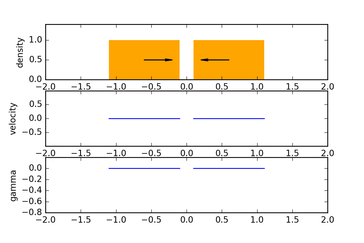
Figure 1: Initial data. The arrows represent the external force $f$ at time $0$.

To illustrate the memory effects of one-dimensional flows in (9d), we consider initial data formed by two congested blocks $\mathbf{1}_{[a_{1},b_{1}]}$ and $\mathbf{1}_{[a_{2},b_{2}]}$ with $b_{1}<a_{2}$ at time $t=0$; see Figure 1. Initially, both the velocity and adhesion potential are equal to zero. We apply an external force $f$, such that the system first compresses and then decompresses in a second phase:

$$f(t,x)=\begin{cases}~{}\alpha\quad&\text{if}\quad x<0\\ ~{}-\alpha\quad&\text{if}\quad x\geq 0\end{cases}\qquad\text{for}\quad t\leq t^{*}$$ (60)

$$f(t,x)=\begin{cases}~{}-\alpha\quad&\text{if}\quad x<0\\ ~{}\alpha\quad&\text{if}\quad x\geq 0\end{cases}\qquad\text{for}\quad t>t^{*}.$$ (61)

In our simulation, we choose $\alpha=0.5$ and $t^{*}=1$. We denote by $X^{\text{ex}}$, $U^{\text{ex}}$ the exact solution of the dynamics. The process can be decomposed into four different phases:

Phase 1. The blocks move freely until time $t_{1}=\sqrt{(a_{2}-b_{1})/\alpha}$. Then the blocks collide. We choose initial positions in such a way that the collision happens at $x=0$:

$$\left\{\begin{aligned} ~{}X^{\text{ex}}_{t}(y)&=X_{0}(y)+\dfrac{\alpha t^{2}}{2}\Big{(}\mathbf{1}_{\{X_{0}(y)<0\}}(y)-\mathbf{1}_{\{X_{0}(y)>0\}}(y)\Big{)}\\ ~{}U^{\text{ex}}_{t}(y)&=\alpha t\Big{(}\mathbf{1}_{\{X_{0}(y)<0\}}(y)-\mathbf{1}_{\{X_{0}(y)>0\}}(y)\Big{)}\\ ~{}\Gamma^{\text{ex}}_{t}(y)&=0\end{aligned}\right.\qquad\text{for $t\leq t_{1}$.}$$

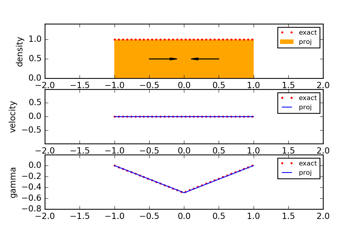
Figure 2: Solution at times $t=t_{1}=0.64$ (left) and $t=t^{*}=1$ (right).

Phase 2. From time $t_{1}$ on, the blocks are stuck together, but the force keeps compressing until time $t=t^{*}$. The velocity is $0$ while the adhesion potential is activated:

$$\left\{\begin{aligned} ~{}X^{\text{ex}}_{t}(y)&=X^{\text{ex}}_{t_{1}}(y)\\ ~{}U^{\text{ex}}_{t}(y)&=0\\ ~{}\Gamma^{\text{ex}}_{t}(y)&=\alpha\big{(}X^{\text{ex}}_{t}(y)-(b_{2}-a_{2})\big{)}t\mathbf{1}_{\{X_{0}(y)>0\}}(y)\\ &-\alpha\big{(}X^{\text{ex}}_{t}(y)+(b_{1}-a_{1})\big{)}t\mathbf{1}_{\{X_{0}(y)<0\}}(y)\end{aligned}\right.\qquad\text{for $t_{1}<t\leq t^{*}$.}$$

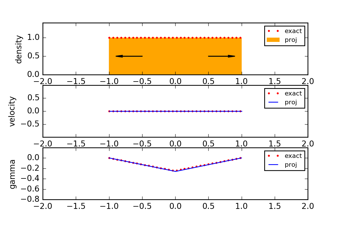
Figure 3: Solution at times $t=1.5$ (left) and $t=t_{2}=2$ (right).

Phase 3. When we reverse the force at time $t=t^{*}$, the blocks remain stuck to each other until the adhesion potential comes back to $0$. The velocity is zero:

$$\left\{\begin{aligned} ~{}X^{\text{ex}}_{t}(y)&=X^{\text{ex}}_{t_{1}}(y)\\ ~{}U^{\text{ex}}_{t}(y)&=0\\ ~{}\Gamma^{\text{ex}}_{t}(y)&=\Big{[}-\alpha\big{(}X^{\text{ex}}_{t}(y)-(b_{1}-a_{1})\big{)}t^{*}\\ &\qquad+\alpha\big{(}X^{\text{ex}}_{t}(y)-(b_{1}-a_{1})\big{)}(t-t^{*})\Big{]}\mathbf{1}_{\{X_{0}(y)<0\}}(y)\\ &+\Big{[}\alpha\big{(}X^{\text{ex}}_{t}(y)-(b_{2}-a_{2})\big{)}t^{*}\\ &\qquad-\alpha\big{(}X^{\text{ex}}_{t}(y)-(b_{2}-a_{2})\big{)}(t-t^{*})\Big{]}\mathbf{1}_{\{X_{0}(y)>0\}}(y)\end{aligned}\right.\qquad\text{for $t^{*}<t\leq t_{2}$.}$$

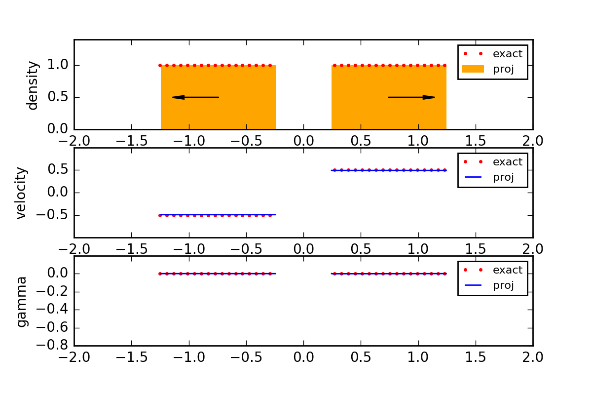
Figure 4: Solution at time $t=3$.

Phase 4. Finally, at time $t_{2}=2t^{*}$ the blocks separate from each other:

$$\left\{\begin{aligned} ~{}X^{\text{ex}}_{t}(y)&=X^{\text{ex}}_{t_{1}}(y)+\dfrac{\alpha(t-t_{2})^{2}}{2}\Big{(}-\mathbf{1}_{\{X_{0}(y)<0\}}(y)+\mathbf{1}_{\{X_{0}(y)>0\}}(y)\Big{)}\\ ~{}U^{\text{ex}}_{t}(y)&=\alpha(t-t_{2})\Big{(}-\mathbf{1}_{\{X_{0}(y)<0\}}(y)+\mathbf{1}_{\{X_{0}(y)>0\}}(y)\Big{)}\\ ~{}\Gamma^{\text{ex}}_{t}(y)&=0\end{aligned}\right.\qquad\text{for $t\geq t_{2}$.}$$

Our numerical code follows the Lagrangian approach developed in the previous sections. To determine the transport $X_{t_{h}}$ at time $t_{h}$, we minimize the objective function

$$\phi_{t_{h}}(X)=\left\|X_{0}+\int_{0}^{t_{h}}{U^{\text{free}}_{s}\,ds}-X\right\|_{L^{2}(\mathbb{R},\rho_{0}}^{2}$$

under the constraint $X\in\widetilde{K}$. This step is performed by use of the Python software CVXOPT for convex optimization; see http://cvxopt.org. We discretize in space by considering the congested blocks consisting of two sets of equally spaced particles of equal mass $m=1.10^{-3}$. The total number of the discrete particles in the system is here $N=2000$. We discretize the time integral of the external force $f$ by the left-hand rectangle method

$$\int_{t_{h}}^{t_{h}+\Delta t}{f(s,X_{s})\,ds}\approx\Delta t\,f(t_{h},X^{\Delta t}_{t_{h}}),$$

where $X^{\Delta}_{t_{h}}\in\mathbb{R}^{N}$ denotes the numerical solution at the discrete time $t_{h}:=h\Delta t$ with $\Delta t>0$. Finally, we express the constraint $X\in\widetilde{K}$ through the linear constraint

$$G\big{(}X^{\Delta t}_{t_{h}}-\widetilde{X}\big{)}\leq\begin{pmatrix}0\\ \vdots\\ 0\end{pmatrix}$$

where the matrix $G\in\mathbb{R}^{N\times N}$ is given by

$$G=\begin{pmatrix}1&-1&~{}&~{}&~{}\\ ~{}&\ddots&\ddots&~{}&~{}\\ ~{}&~{}&\ddots&\ddots&~{}\\ ~{}&~{}&~{}&\ddots&-1\\ ~{}&~{}&~{}&~{}&1\end{pmatrix}.$$

We represent in Figures 2 and 4 our numerical solution during the four phases of the process. We observe excellent agreement between the numerical solution and the exact solution.

5 Extension to heterogeneous maximal constraint

We consider the case where in the maximal density constraint, the upper bound is replaced by a function, so that $0\leq\rho\leq\rho^{*}$, where $\rho^{*}$ is transported with the flow. Thus

$$\partial_{t}\rho+\partial_{x}(\rho u)=0$$ (62a)

$$\partial_{t}(\rho u-\partial_{x}\gamma)+\partial_{x}\big{(}(\rho u-\partial_{x}\gamma)u\big{)}=\rho f$$ (62b)

$$\partial_{t}\rho^{*}+u\partial_{x}\rho^{*}=0$$ (62c)

$$0\leq\rho\leq\rho^{*}$$ (62d)

$$(\rho^{*}-\rho)\gamma=0,\quad\gamma\leq 0.$$ (62e)

This system has been studied by Degond et al. [11] in the Navier-Stokes framework. At initial time we prescribe, in addition to $\rho_{0},u_{0}$, and $\gamma_{0}$, the initial constraint $\rho^{*}_{0}$ so that $\rho_{0}\leq\rho^{*}_{0}$ a.e. in $\mathbb{R}$. Combining (62a) with (62c), we observe that the ratio $r:=\rho/\rho^{*}$ is conserved:

$$\partial_{t}r+\partial_{x}(ru)=0.$$ (63)

We now consider $r$ instead of $\rho$ and look for a monotone transport map $Y_{t}$ such that

$$r_{t}=(Y_{t})_{\#}r_{0}.$$

We reformulate the system (62e) in the form

$$\partial_{t}r+\partial_{x}(ru)=0$$ (64a)

$$\partial_{t}(ru-\partial_{x}\gamma)+\partial_{x}\big{(}(ru-\partial_{x}\gamma)u\big{)}=\rho f$$ (64b)

$$\partial_{t}\rho^{*}+u\,\partial_{x}\rho^{*}=0$$ (64c)

$$0\leq r\leq 1$$ (64d)

$$(1-r)\gamma=0,\quad\gamma\leq 0.$$ (64e)

This transport $Y_{t}$ has thus to satisfy the constraint $Y_{t}\in\widetilde{K}$ with $\widetilde{K}:=K+\widetilde{Y}$. Here $K$ is again the cone of monotone transport maps, and $\widetilde{Y}\in K$ is the uniquely determined transport map with $\widetilde{\rho}=\widetilde{Y}_{\#}r_{0}$, where $\widetilde{\rho}$ is the same as in (24). By replacing the density $\rho$ by the ratio $r=\rho/\rho^{*}$ in the proof presented in the previous sections, we can define exactly in the same way as before a Lagrangian velocity $U_{t}=\frac{d}{dt}Y_{t}$ and an adhesion potential such that

$$\bar{r}(y)\bar{U}(y)=\bar{r}(y)\bigg{(}U_{t}(y)-\int_{0}^{t}f(s,Y_{s}(y))\,ds\bigg{)}-\partial_{y}\Gamma_{t}(y).$$

for a.e. $y\in\mathbb{R}$ and $t\in(0,T)$, with $\bar{r},\bar{U}$ suitable initial data. One can then check that we have constructed a global weak solution to the heterogeneous system (64e).

Theorem 5.1.

Let $T>0$ and external force $f\in L^{\infty}\big{(}0,T;\mathrm{Lip}(\mathbb{R})\cap L^{\infty}(\mathbb{R})\big{)}$ be given. Suppose that $\bar{\rho},\rho_{0}^{*}\in\mathcal{P}_{2}(\mathbb{R})$ with $\bar{\rho},\rho_{0}^{*}\ll\mathcal{L}^{1}$ and $\rho_{0}^{*}>0$ a.e., and assume that

$$0\leq\bar{\rho}\leq\rho_{0}^{*}\quad\text{a.e. in $\mathbb{R}$.}$$

It follows that $r_{0}:=\rho_{0}^{*}/\bar{\rho}\leq 1$. Let $\bar{u}\in L^{2}(\mathbb{R},\bar{\rho})$ and define

$$\rho_{0}:=\bar{\rho},\quad U_{0}:=\bar{u},\quad Y_{0}:=\mathrm{id}.$$

There exists a curve $[0,T]\ni t\mapsto Y_{t}\in\widetilde{K}$ that is differentiable for a.e. $t\in(0,T)$ and solves

$$Y_{t}=\mathrm{P}_{\widetilde{K}}\left(Y_{0}+\int_{0}^{t}{U^{\text{free}}_{s}\,ds}\right),\quad U^{\text{free}}_{t}=U_{0}+\int_{0}^{t}f(s,Y_{s})\,ds.$$

The following quantities are well-defined: $\rho^{*}_{t}(x):=\rho^{*}_{0}(Y_{t}^{-1}(x))$ for a.e. $x\in\mathbb{R}$, and

$$U_{t}(y):=\dot{Y}_{t}(y),\quad\Gamma_{t}(y):=\int_{-\infty}^{y}{\Big{(}U_{t}(z)-U^{\text{free}}_{t}(z)\Big{)}r_{0}(z)\,dz}$$

for $y\in\mathbb{R}$ and a.e. $t\in(0,T)$. There exist $(u_{t},\gamma_{t})\in\mathcal{L}^{2}(\mathbb{R},r_{t})\times W^{1,1}(\mathbb{R})$, such that

$$U_{t}=u_{t}\circ X_{t},\quad\Gamma_{t}=\gamma_{t}\circ X_{t},$$

where $r_{t}:=(X_{t})_{\#}r_{0}$. The tuple $(r,u,\gamma,\rho^{*})$ is a global weak solution of system (64e).

Numerical simulation.

We consider the following initial data (see Figure 5):

$$\rho^{*}_{0}(x)=1+0.2*\big{(}1-\cos(2\pi(x-0.5))\big{)},$$

$$\rho_{0}(x)=0.8\,\rho^{*}_{0}(x)\,\mathbf{1}_{[0,1]}(x).$$

We add a compressive external force such that

$$f(x)=\begin{cases}+0.5\quad&\text{if $x<0.5$}\\ -0.5\quad&\text{if $x>0.5$,}\end{cases}$$

which tends to concentrate the density at the middle of the interval $[0,1]$. We set the particle mass $m=1.10^{-3}$, so that $N=1000$ discrete particles are used in the simulation. We display in Figures 5 and 6 the concentration phenomenon with the appearance of a congested zone where the velocity is equal to $0$ and the adhesion potential is negative.

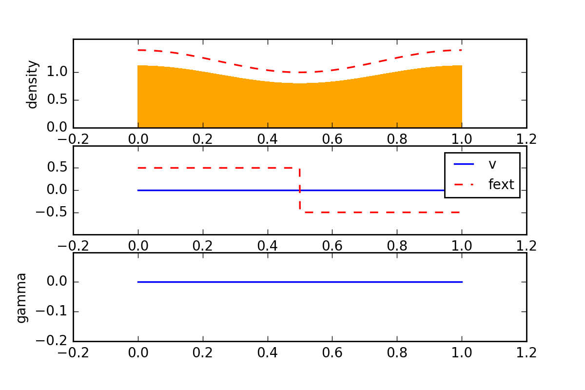
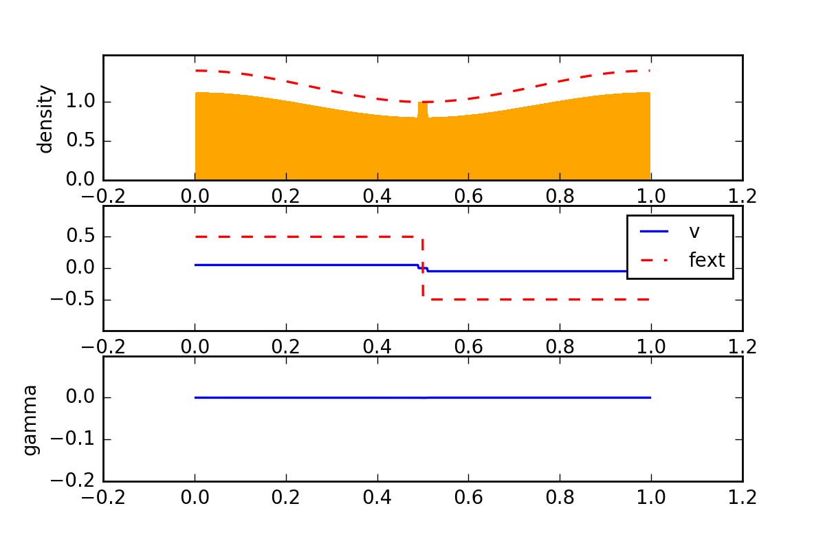
Figure 5: Variable maximal density: solution at times $t=0$ (left) and $t=0.1$ (right).

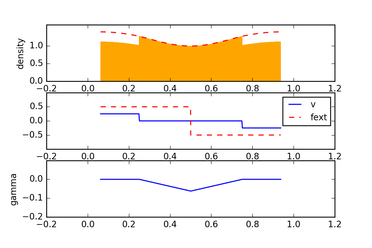
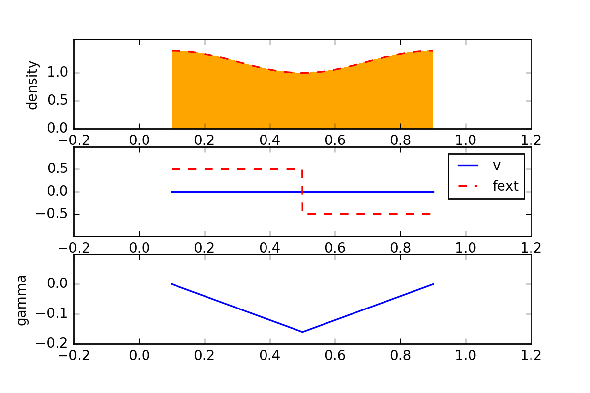
Figure 6: Variable maximal density: solution at times $t=0.5$ (left) and $t=0.8$ (right).

References

- [1] Ambrosio, L., Fusco, N., and Pallara, D. Functions of bounded variation and free discontinuity problems. The Clarendon Press Oxford University Press, 2000.
- [2] Ambrosio, L., Gigli, N., and Savaré, G. Gradient flows: in metric spaces and in the space of probability measures. Springer Science & Business Media, 2008.
- [3] Bainov, D. D., and Simeonov, P. S. Integral inequalities and applications, vol. 57. Springer Science & Business Media, 2013.
- [4] Berthelin, F. Existence and weak stability for a pressureless model with unilateral constraint. Mathematical Models and Methods in Applied Sciences 12, 02 (2002), 249–272.
- [5] Bouchut, F. On zero pressure gas dynamics, advances in kinetic theory and computing, 171-190. Ser. Adv. Math. Appl. Sci 22 (1994).
- [6] Bouchut, F., Brenier, Y., Cortes, J., and Ripoll, J.-F. A hierarchy of models for two-phase flows. Journal of NonLinear Science 10, 6 (2000), 639–660.
- [7] Boudin, L. A solution with bounded expansion rate to the model of viscous pressureless gases. SIAM Journal on Mathematical Analysis 32, 1 (2000), 172–193.
- [8] Brenier, Y., Gangbo, W., Savaré, G., and Westdickenberg, M. Sticky particle dynamics with interactions. Journal de Mathématiques Pures et Appliquées 99, 5 (2013), 577–617.
- [9] Brenier, Y., and Grenier, E. Sticky particles and scalar conservation laws. SIAM journal on numerical analysis 35, 6 (1998), 2317–2328.
- [10] Cavalletti, F., Sedjro, M., and Westdickenberg, M. A simple proof of global existence for the 1d pressureless gas dynamics equations. SIAM Journal on Mathematical Analysis 47, 1 (2015), 66–79.
- [11] Degond, P., Minakowski, P., and Zatorska, E. Transport of congestion in the two-phase compressible/incompressible flow. Nonlinear Analysis: Real World Applications, Elsevier 42 (2018), 485–510.
- [12] Degond, P., Minakowski, P., Navoret, L. and Zatorska, E. Finite Volume approximations of the Euler system with variable congestion. Computers & Fluids, Elsevier 169 (2018), 23|-39.
- [13] Jabin, P.-E., and Rey, T. Hydrodynamic limit of granular gases to pressureless Euler in dimension 1. Quart. Appl. Math. 75 (2017), no.1, 155–179.
- [14] Lannes, D. On the dynamics of floating structures. Annals of PDE, Springer 3.1 (2017),11.
- [15] Lefebvre, A. Modélisation numérique d’écoulements fluide-particules: prise en compte des forces de lubrification. PhD thesis, Université de Paris-Sud. Faculté des Sciences d’Orsay (Essonne), 2007.
- [16] Lefebvre-Lepot, A., and Maury, B. Micro-macro modelling of an array of spheres interacting through lubrication forces. Advances in Mathematical Sciences and Applications 21, 2 (2011), 535.
- [17] Maury, B. A gluey particle model. In ESAIM: Proceedings (2007), vol. 18, EDP Sciences, pp. 133–142.
- [18] Maury, B., and Preux, A. Pressureless Euler equations with maximal density constraint : a time-splitting scheme. https://hal.archives-ouvertes.fr/hal-01224008 (2015).
- [19] Natile, L., and Savaré, G. A wasserstein approach to the one-dimensional sticky particle system. SIAM Journal on Mathematical Analysis 41, 4 (2009), 1340–1365.
- [20] Perrin, C. Modelling of phase transitions in one–dimensional granular flows. ESAIM: Proceedings and Surveys, 58 (2017), 78–97.
- [21] Perrin, C. Pressure-dependent viscosity model for granular media obtained from compressible Navier–Stokes equations. Applied Mathematics Research eXpress 2016, 2 (2016), 289–333.
- [22] Perrin, C., and Zatorska, E. Free/congested two-phase model from weak solutions to multi-dimensional compressible Navier-Stokes equations. Communications in Partial Differential Equations 40, 8 (2015), 1558–1589.
- [23] Preux, A. Transport optimal et équations des gaz sans pression avec contrainte de densité maximale. Theses, Université Paris-Sud, Nov. 2016.
- [24] Rachev, S.T., and Rüschendorf, L. Mass transportation problems, vol 1 Probability and its Applications, Springer-Verlag, New York, 1998. Theory.
- [25] Santambrogio, F. Optimal transport for applied mathematicians, vol. 87. Springer, 2015.
- [26] Sobolevskii, A. N. The small viscosity method for a one-dimensional system of equations of gas dynamic type without pressure. Dokl. Akad. Nauk 356, 3 (1997), 310–312.
- [27] Wolansky, G. Dynamics of a system of sticking particles of finite size on the line. Nonlinearity 20, 9 (2007), 2175.
- [28] Zel’Dovich, Y. B. Gravitational instability: An approximate theory for large density perturbations. Astronomy and astrophysics 5 (1970), 84–89.