Muon Counting using Silicon Photomultipliers in the AMIGA detector of the Pierre Auger Observatory

Abstract

AMIGA (Auger Muons and Infill for the Ground Array) is an upgrade of the Pierre Auger Observatory designed to extend its energy range of detection and to directly measure the muon content of the cosmic ray primary particle showers. The array will be formed by an infill of surface water-Cherenkov detectors associated with buried scintillation counters employed for muon counting. Each counter is composed of three scintillation modules, with a 10 m² detection area per module. In this paper, a new generation of detectors, replacing the current multi-pixel photomultiplier tube (PMT) with silicon photo sensors (aka. SiPMs), is proposed. The selection of the new device and its front-end electronics is explained. A method to calibrate the counting system that ensures the performance of the detector is detailed. This method has the advantage of being able to be carried out in a remote place such as the one where the detectors are deployed. High efficiency results, i.e. 98 % efficiency for the highest tested overvoltage, combined with a low probability of accidental counting ($\sim$2 %), show a promising performance for this new system.

1 Introduction

The Pierre Auger Obsevatory [1] is located in the province of Mendoza, Argentina and has an area of 3000 km². It was designed to detect ultra-high energy cosmic ray showers with a hybrid detection technique. It has 1660 surface water-Cherenkov detector stations (SDs) [2] arranged in a triangular grid with a distance of $\sim$1.5 km between stations, and 27 fluorescence detector (FD) telescopes [3] at four sites on the periphery of the array pointing towards the atmosphere and the center of the array. The Auger Observatory is currently being upgraded, and AMIGA [4, 5, 6] (Auger Muons and Infill for the Ground Array) is one of its principal enhancements. Two of the main objectives of AMIGA are the measurement of composition-sensitive observables of extensive air showers and the study of features of hadronic interactions. Important results on cosmic ray physics by means of muon detection techniques have been previously obtained by several experiments like KASCADE [7] and KASCADE-Grande [8].

AMIGA consists of 61 detector pairs, each one composed of a SD station and a 30 m² muon counter, deployed on a 750 m triangular grid in an infilled area of 23.5 km². At the Observatory site, the associated SD triggers the muon counter (MC) when a candidate cosmic ray shower is measured. Each muon counter is buried 2.3 m underground to shield the electromagnetic component of cosmic ray showers (vertical shielding of 540 g/cm²) and it is composed of three scintillation modules. Every module comprises 64 scintillation bars, each of dimensions 400 cm x 4 cm x 1 cm, with a 1.2 mm diameter wavelength-shifting (WLS) optical fiber (BCF-99-29AMC) glued to a lengthwise groove on each bar. The light produced in the bars is absorbed by the WLS fiber. The excited molecules of the fiber decay while emitting photons, some of which are propagated along the WLS fibers towards a channel of a multi-pixel photon detector. The aim of these modules is to efficiently count the number of muons that impinge on the 10 m² area of scintillation. The mechanical detector design is fixed and detailed in [9]. An engineering array of seven muon counters with multi-pixel photomultiplier tubes (PMTs) is already installed and acquiring data at the Observatory site.

For the production of AMIGA the current PMTs are going to be replaced with silicon photo sensors (aka. SiPMs). The main motivations for this upgrade are the advantages of these devices compared to current PMTs: their lower cost per channel, longer life-time, better sturdiness, higher photon detection efficiency at the optical fiber emission wavelength, and no optical cross-talk between channels. The main disadvantages of SiPMs are its higher noise rate and temperature dependence. In this paper is explained how, with the proposed electronics and calibration method, these disadvantages are addressed.

The present paper is organized as follows: a general description of the SiPM behavior is detailed in section 2. Then the SiPM and the front-end electronics selection is explained in section 3. The proposed calibration of the counting system is described in section 4. Finally, the efficiency measurements are shown in section 5.

2 The Silicon Photomultiplier

A SiPM [10] is a solid-state device capable of detecting individual photons. It is composed of an array of cells, all connected in parallel. Each cell has an avalanche photo-diode (APD) working in Geiger mode and a quenching resistor ($R_{Q}$) in series (see figure 1).

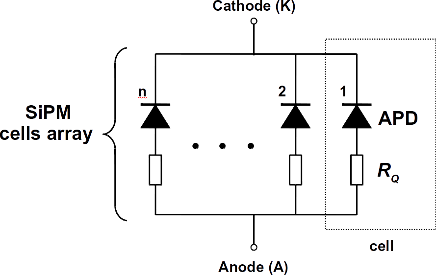
Figure 1: Schematic view of the internal structure of a SiPM made up of an array of cells, all connected in parallel. Each cell is composed of an APD working in Geiger mode and a quenching resistor ($R_{Q}$) in series.

The APD starts working in Geiger mode when the reverse voltage ($V_{bias}$) applied to it exceeds a specific voltage value called the breakdown voltage ($V_{BR}$). In this mode the injection of a single charge carrier (e.g. due to an impinging photon) causes a self-sustained avalanche. The current that flows through the APD depends on the voltage value over the breakdown which is called overvoltage ($\Delta V=V_{bias}-V_{BR}$). The flow of this current through $R_{Q}$ produces the decrease of the reverse voltage ($V_{APD}$) applied to the APD. When $V_{APD}$ is below $V_{BR}$ the avalanche is extinguished. This last sequence describes the “firing” of a cell. From now on, the signal produced by this firing process will be called single photon equivalent (SPE). If multiple cells are fired simultaneously the resulting output signal will be a superposition of SPEs. The amplitude of this signal will be directly proportional to the number of fired cells.

As was previously mentioned, SiPMs are employed to detect photons. An undesirable effect is the accidental counting of those photons due to noise in the cells. In the next subsection, the sources of noise are defined.

2.1 SiPM Noise

Noise in SiPMs [11] is defined as the firing of a cell that was not produced by a photon impinging the device. There are three noise sources which can be separated in two types, depending on the correlation or not with the firing of a cell.

2.1.1 Uncorrelated Noise: Dark Noise

Dark noise occurs randomly due to thermally-generated charge carriers (electron-hole pairs) either in the depletion region or in the avalanche region [12]. The amplitude and shape of these pulses are the same as the ones produced by the absorption of a photon. Dark noise is sensitive to temperature, and also depends on the array size, overvoltage magnitude, and semiconductor material quality.

2.1.2 Correlated Noise: Afterpulsing and Cross-Talk

Afterpulsing is a secondary avalanche produced after the firing of a cell, due to the release of trapped charges. The release of these trapped charges occurs after a characteristic time that depends on the type of the trapping centers and its occurrence probability decreases exponentially with time. It is noise correlated to the firing of a cell and it is produced in the same cell.

When a primary avalanche in a cell produces photons with energy greater than the band gap energy, there is a probability that a nearby cell absorbs the photon, producing its firing. As a first order approximation, the secondary avalanche is synchronized in time with the main primary avalanche to produce a resulting signal of a channel with an increased amount of SPEs stacked. This effect is called cross-talk.

3 Proposed Readout for AMIGA Muon Counters

As mentioned in the Introduction, for the production of AMIGA, the current PMTs are going to be replaced with SiPMs. The mechanical module design is already fixed. One of the characteristics that constrains the proposed readout for AMIGA muon counters is its segmentation. The detector is segmented, in space as well as in time, to prevent undercounting due to simultaneous muon arrivals:

• Segmentation in space. Based on simulations [13], each of the three scintillator modules of a muon counter has been segmented into 64 segments.

• Segmentation in time. This segmentation is limited by the time distribution of the photons produced by the impinging particle. This time distribution is defined by the convolution of the probability distributions characterized by the decay time of the scintillator, the decay time of the optical fiber, and to a lesser extent the propagation mode in the optical fiber. The maximum time width of a light signal for AMIGA MCs is between 25 to 35 ns [14].

The proposed electronics of the module must facilitate the identification of pulses above a given threshold to allow muon counting, without knowing in detail the signal structure and peak intensity. The proposed readout must not degrade the detector segmentation.

A SiPM model and new electronics for the readout of AMIGA MCs are proposed in the next two subsections, based on the experience of the current version of the AMIGA electronics [15, 16].

3.1 SiPM Selection

Two main features which improve the signal-to-noise ratio were taken into account in order to select the specific device: high photo-detection efficiency (PDE) and low noise. The PDE of the selected devices is around 35 % for the peak emission wavelength of the fiber optic (485 nm). Low noise is obtained by combining low dark rate with reduced cross-talk and low afterpulsing probability.

Three devices manufactured by Hamamatsu (S12572-100C, S12571-100C, S13081-050CS) were tested in the laboratory to evaluate their performance. In Figure 2 an overlap of 5000 dark rate traces of each SiPM model is shown. Pulses of more than one SPE, stacked due to cross-talk, can be observed synchronized with the trigger time. Afterpulsing pulses can also be observed after the trigger time.

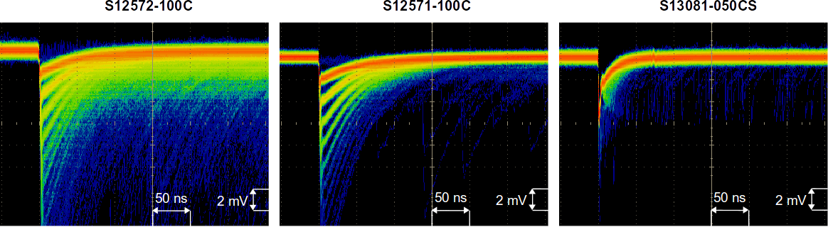
Figure 2: Overlap of 5000 dark rate traces (signal amplitude as a function of time) of each SiPM model. All measurements were done with the same amplifier at 25 ^∘C. The $\Delta V$ of each SiPM was set to the value recommended by Hamamatsu.

The three SiPMs exemplified are some of the latest devices developed by Hamamatsu up to 2015. The second SiPM (S12571-100C) in figure 2 shows a reduction in the afterpulsing probability compared to the first one (S12572-100C). The third model (S13081-050CS) not only shows a reduction in the afterpulsing, but also a significantly lower value of cross-talk. The main characteristics of these SiPMs, obtained from the Hamamtsu datasheets, are summarized in table 3.1.

The criteria selected for counting muons is to count pulses above a given threshold. In this context, cross-talk probability becomes a relevant parameter. This correlated noise makes possible that a pulse triggered by dark noise or afterpulsing could have an amplitude above the selected threshold. Therefore, cross-talk should be as small as possible to reduce the accidental counting probability. The selected device for this work was the third model (S13081-050CS) mainly due to its low cross-talk probability and also its low dark noise and afterpulsing.

Table 3.1: Main characteristics, obtained from the Hamamatsu datasheets, of the three tested SiPMs: S12571-100C [17], S12572-100C [18] and S13081-050CS.

Parameter		SiPM Model			Unit
		S12572-100C	S12571-100C	S13081-050CS
Cell Pitch		100	100	50	$\mu$m
Effective Photosensitive Area		3 x 3	1 x 1	1.3 x 1.3	mm
Geometrical Fill Factor		78.5	78	61	%
Photon Detection Efficiency		35	35	35	%
Number of Cells		900	100	667	-
Dark Count	Typ.	1000	100	90	kcps
	Max.	2000	200	360	kcps
Gain M (at operation voltage)		2.8 x 106	2.8 x 106	1.5 x 106	-
Gain Temperature Coefficient		1.2 x 105	1.2 x 105	2.7 x 104	${}^{\circ}C^{-1}$
Breakdown Voltage		65 $\pm$ 10	65 $\pm$ 10	53 $\pm$ 5	V
Cross-Talk Probability		35	35	1	%
Temperature Coefficient		60	60	54	mV$/^{\circ}C$

3.2 Proposed Electronics

The proposed electronics is based on the existing AMIGA system. The following main specifications were considered for the design:

1. The new electronics design must be compatible with the existing mechanical design of the detector. There is no access to the optical fibers, only to the optical connector. Fibers of 1.2 mm diameter are glued to the optical connector in a squared arrangement of 8$\times$8 and the separation distance between two neighboring fibers centers is 2.3 mm.

2. The electronics must be able to identify light pulses with a maximum time width between 25 to 35 ns. This upper limit is obtained from the light pulses time width distribution. This distribution is the result of the convolution of the probability distributions characterized by the decay time of the scintillator, the decay time of the optical fiber, and to a lesser extent the propagation mode in the optical fiber.

3. Low power consumption (stand-alone power system).

4. The output of each SiPM channel must be a digital 0-1 signal to allow muon counting. The digital output width must be similar to the characteristic time width of the light pulses produced in the detector. Wider digital signals are not desired since the detection of consecutive muons in the same bar could be deteriorated (pile-up effect).

5. Temperature compensation (SiPM breakdown voltage depends on temperature).

The Application Specific Integrated Circuit (ASIC) Cherenkov Imaging Telescope Integrated Read Out Chip (CITIROC) [19] was proposed for the front-end readout of AMIGA. The CITIROC ASIC is a 32 channel front-end specially designed for the readout of SiPMs. An adjustment of the SiPM biasing is possible using a channel-by-channel 8-bit digital-to-analog converter (DAC) connected to the ASIC inputs. Each channel has a pre-amplifier stage that can be selected by software between a low or high gain pre-amplifier. Also each corresponding gain value is programmable. Then the signal passes through a 15 ns peaking time fast shaper followed by a discriminator. The discriminator threshold is set coarsely by a 10-bit DAC (common for the 32 channels) and then set finely channel by channel by individual 4-bit DACs. The 15 ns peaking time fast shaper enables a digital output width of the discriminator similar to the characteristic time width of the light pulses produced by the impinging particles in the detector. The fast shaper produces an undesirable effect. It has a negative overshot which might influence the detection efficiency for the next close in time muon. The capability to detect two consecutive muons is not within the scope of this work. This effect and others like larger signal time width, due to the WLS fiber decay time, and the recovery time of cells in the SiPM, must be studied further in the future.

For the biasing and temperature compensation of each SiPM, the Hamamatsu C11204-01 power supply [20] was selected due to the recommendation of Hamamatsu. This power supply has one output with low ripple noise (0.1 mVp-p typ.), good temperature stability ($\pm$10 ppm/^∘C typ.) and a high output voltage resolution (1.8 mV).

4 Calibration Method of the Counting System

The calibration method of the counting system for AMIGA is split into two steps. The first step consists in calibrating the optical sensors of each individual channel (see subsection 4.1) and the second step consists in calibrating the detector (see subsection 4.2).

4.1 SiPM Calibration

The goal of this calibration is to set the operation point of the SiPMs. First, the breakdown voltage of each individual channel must be obtained. Then, all the SiPMs must be biased to its corresponding breakdown voltage with an added pre-determined overvoltage. This overvoltage can be changed to optimize the efficiency. In this section a method for obtaining the breakdown voltage and biasing of the SiPMs with the proposed AMIGA electronics is explained.

4.1.1 SiPM Calibration Setup

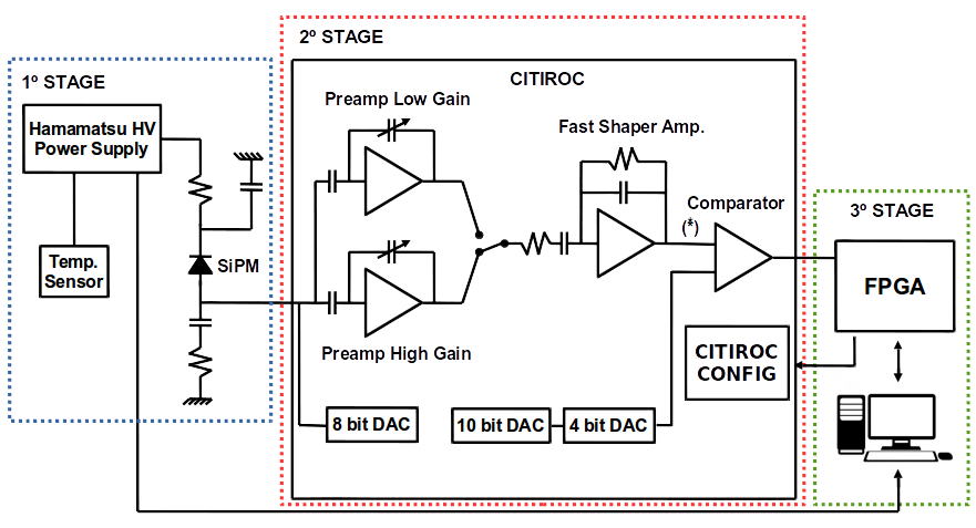
Figure 3: SiPM Calibration Setup. The three stages are distinguished with dotted lines. The output of the fast shaper amplifier ($\ast$) has a DC offset component.

The setup for the SiPMs calibration is divided into three stages (see figure 3). The first stage is composed of the SiPM, the high voltage power supply and the temperature sensor. Since the SiPM breakdown voltage varies significantly with temperature, the high voltage power supply has a built-in high precision temperature compensation system that constantly corrects the SiPM operation point. This function tries to keep the gain value fixed independently of temperature variations. The compensation of the high voltage ($HV$) output of the power supply is determined by the following equation given by Hamamatsu:

$$HV=K_{2}*(T-T_{ref})^{2}+K_{1}*(T-T_{ref})+V_{ref}$$ (4.1)

In this formula, the $K_{2}$ and $K_{1}$ are respectively the quadratic and linear coefficients for the temperature compensation, $V_{ref}$ is the reference voltage and $T_{ref}$ is the reference temperature. The temperature compensation for the SiPMs under test is linear and the quadratic term is not needed. The $K_{2}$ was set to 0 mV/^∘C², $K_{1}$ to 54 mV/^∘C (see table 3.1) and $T_{ref}$ to 25 ^∘C. The resulting formula for the calibration is:

$$HV=54\,mV/^{\circ}C*(T-25\,^{\circ}C)+V_{ref}$$ (4.2)

The second stage consists of the CITIROC. This stage amplifies and then discriminates SiPM pulses. The chip was programmed to use the high gain pre-amplifier, with its maximum gain value of 150, to improve the separation between SPEs in the SPE spectrum. The 8-bit DAC was set to a fixed value (e.g. 250 dac-units). The 10-bit DAC was used to set the comparator threshold for all the channels and the 4-bit DAC of each channel was fixed to its minimum value.

The third stage is composed of an Altera Cyclone IV FPGA. The FPGA was programmed to measure the rate of the CITIROC digital pulses output.

4.1.2 Single Photon Equivalent Peak Measurement

A dedicated software was developed to automatically measure the rate of the digital pulses at different discrimination levels. In the measurement of the SiPM noise rate as a function of the 10-bit DAC values (see figure 4, left) there is a clear transition from the first to the second plateau. This transition is required for the calibration and it represents the threshold of the comparator passing through the first SPE peak.

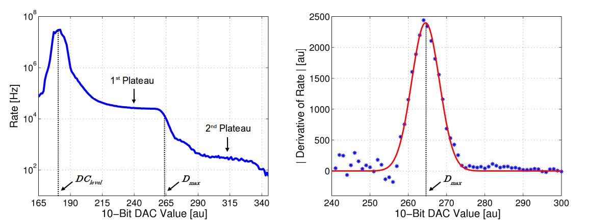
Figure 4: On the left, the measurement of the rate of the SiPM pulses as a function of the DAC value. $DC_{level}$ corresponds to the fast shaper DC offset component. See subsection 4.1.1 for details on the setup. On the right, the absolute value of the derivative of the rate evidences the distribution of the SPE peaks. The mean value of the SPE peak ($D_{max}$) is obtained with a Gaussian fit of the points (red curve).

The absolute value of the derivative of this curve (see figure 4, right) represents the distribution of the SPE peak values. The mean value of the SPE peak ($D_{max}$) is correlated to the maximum absolute value of the Gaussian distribution coming from the derivative of the rate curve. This value has an offset ($DC_{level}$) because the signal in the fast shaper has a DC offset component (see figure 3). The value of this DC offset is the DAC value where the rate is maximum (see figure 4, left). To obtain the real value of the SPE peak ($SPE_{peak}$) it is necessary to subtract this offset.

$$SPE_{peak}=D_{max}-DC_{level}$$ (4.3)

As was mentioned before, the employment of SiPMs combined with the method explained in this subsection, allow the $SPE_{peak}$ estimation which is used to calculate the breakdown voltage of the device, as it will be explained in the next subsection.

4.1.3 Breakdown Voltage Measurements

There are several methods to estimate the breakdown voltage of a SiPM [21]. Due to the constraints of the proposed electronics, the method to estimate each channel breakdown voltage is the one described in this subsection.

The total charge produced in an avalanche can be calculated using equation 4.4 and the gain ($M$) of this process is defined by equation 4.5.

$$Q=C_{j}\Delta V$$ (4.4)

$$M=Q/e\hskip 14.22636pt\textrm{where}\ e\ \textrm{is the electron charge.}$$ (4.5)

It can be inferred from these equations that the gain depends linearly on the overvoltage. Therefore, for the special case when the gain is zero, $V_{bias}=V_{BR}$. The functional dependencies described by these equations are shown in figure 5, left. This figure shows that if the gain ($M$) is measured over the $V_{bias}$, the breakdown voltage can be obtained as the value where the curve intercepts the X axis ($V_{bias}=V_{BR}$). It is also known that the $SPE_{peak}$ is directly proportional to the gain (Mean $SPE_{peak}$ $\varpropto$ M). By using this information and following the procedure explained in the previous subsection, a plot of $SPE_{peak}$ for different $V_{bias}$ values, can be obtained. An example for four different SiPMs is shown in figure 5, right. From that plot, the $V_{BR}$ can be estimated as the point where the linear fit of the curve intercepts the X axis ($V_{bias}=V_{BR}$).

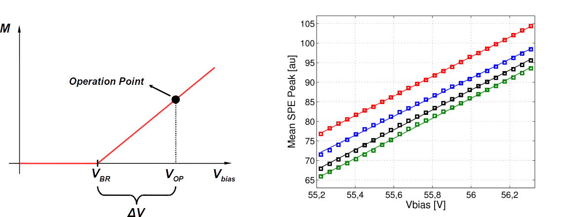
Figure 5: Equations 4.4 and 4.5 are presented graphically in the plot on the left. The mean $SPE_{peak}$ as a function of the $V_{bias}$ for four different SiPMs is plotted on the right. The mean $SPE_{peak}$ is proportional to $M$.

To automatize the breakdown voltage estimation, the 8-bit DAC of the CITIROC (see figure 3) was fixed to 250 dac-units for all the channels and the HV value was modified in regular steps ($V_{bias}$ changes following the power supply HV). With this method, each SiPM characteristic breakdown voltage was calculated at the same time, with a single power supply. This is required for the AMIGA design since the 64 channels of each module are connected to the same power supply. In the following subsection a possible equalization of SiPMs overvoltage is explained following this constraint.

4.1.4 Equalization Between Channels

The equalization consists in applying the same $\Delta V$ to all the 64 channels of one module. This equalization does not ensure the same gain or rate at a given threshold between channels. To set the operation voltage for each channel, considering that each SiPM has a different breakdown voltage ($V_{BR_{i}}$), the following procedure is carried out:

1. Set the $HV$ voltage of the power supply to the largest $V_{BR_{i}}$ ($V_{BR_{max}}$) of the 64 SiPMs with the desired $\Delta V$ added. $HV=V_{BR_{max}}+\Delta V$.

2. Set the 8-bit DAC of each CITIROC channel following: $V_{8bitDAC}=V_{BR_{max}}-V_{BR_{i}}$.

4.2 Detector Calibration

Once the SiPM is calibrated, the next step consists of determining the discrimination level and the counting strategy (detector calibration), ensuring an adequate performance of the counting system.

4.2.1 Detector Calibration Setup

The setup for the detector calibration is divided into six stages (see figure 6). The first and second stages were described in subsection 4.1.1. For this calibration, the CITIROC was programmed to use the high gain pre-amplifier with its minimum gain value of ten to reduce the digital time span of the discriminated pulses. The individual channel threshold DAC (4-bit DAC) was fixed to its minimum value and the high voltage adjustment DAC (8-bit DAC) was set following the procedure detailed in the subsection 4.1.4 (equalization). The common chip threshold adjustment DAC (10-bit DAC) is used to set different discrimination levels. The third stage is a wide-band amplifier with a gain value of ten, to allow the measurement of the analog signal of the SiPM. The fourth stage consists of a 4 m plastic scintillation bar with a threaded 5 m wavelength-shifting optical fiber, built identically to the scintillator strips that conform an AMIGA muon counter. At the end of the optical fiber there is an optical connector coupled to the SiPM. The extra meter of fiber is between the scintillator and the SiPM. The fifth stage is an ad-hoc muon telescope trigger [22] which triggers the acquisition every time a particle passes through each position of the main scintillating bar where the telescope is placed. It consists of two identical parts, each of them made of a scintillator of dimensions 4 cm x 4 cm x 1 cm with a SiPM coupled for light detection. Both pieces are aligned above and below the main scintillating bar. The separation distance between triggers is 5 cm and the main scintillating bar is placed equidistantly between both parts. This configuration selects a particular solid angle of the muons that impinges the main scintillator. The trigger condition is overcome when the two SiPMs, up and down, record signals above a given threshold in a time-coincidence window of 60 ns. There is a probability of $\sim$2 % of false coincidences of this muon telescope mainly due to three factors: the probability of two different particles impinging each scintillator simultaneously without passing, neither of them, through the main scintillator, misalignment of the telescope with respect to the main scintillator, and simultaneous dark noise at both devices. The sixth stage is the acquisition system. This stage is composed of a Tektronix DPO7104 oscilloscope. This oscilloscope is set up to store the discriminated signal of the CITIROC (second stage) and the amplified analog signal of the SiPM (third stage) every time the muon telescope produces a coincidence in a time window of 60 ns (fifth stage).

Figure 6: The six stages of the setup needed for the detector calibration. The 4 m plastic scintillation bar has a threaded 5 m wavelength-shifting optical fiber. The difference in length is due to the extra fiber needed to reach the optical connector.

4.2.2 Selection of the Counting Strategy

As was described in [23], the current counting system (PMT and electronics) has been designed to count muons by identifying a pattern in the digital trace of a fixed length of 3.2 $\mu$s. The length of the digital trace is fixed by the cosmic ray shower duration. The discrimination level is set to a value lower than one SPE and then a pattern recognition technique is applied to discriminate particles from noise. This counting strategy takes into account the time structure of the signal over a threshold.

The proposed counting strategy for the SiPMs is based on an amplitude criteria. The high noise of SiPMs implies setting a threshold of a small number of SPEs to discriminate particles from noise. The high PDE ($\sim$35 %) of SiPM at the emission wavelength of the WLS optical fiber mitigates the loss of detection efficiency.

The discrimination level is set to the lowest value that ensures a low rate of contamination (negligible accidental counting) without significantly reducing the counting efficiency. In figure 7, the rate of SiPM pulses as a function of the 10-bit DAC threshold is shown. For these measurements the muon telescope was not used and the rate is acquired directly from the CITIROC digital output with a pulse counter programmed in the FPGA. Two cases are plotted: the red complete line is the rate when the fiber is coupled to the SiPM, and the blue dashed line when it is not. When the fiber is not coupled to the SiPM, only the noise from the SiPM is measured. When the fiber is coupled to the SiPM, not only the dark rate and its correlated noise are measured, but also all the signals produced by charged particles impinging the scintillator. These particles will be considered as the environmental radiation. This environmental radiation is composed of cosmic ray particles (muons and others) and radiation of the surrounding materials (e.g. walls, floor, casing). In figure 7, for one and two SPE rate levels, the correlated and the uncorrelated noises, explained in section 2.1, dominate. If the threshold level is set to any of these values, the accidental counting probability for the whole detector (64 channels) is over the desired limit level of 5 %. This 5 % was selected considering that the overcounting must remain below the error value of the number of muons reported in [24], see Figures 5, 8, and 11. At three SPE rate level, the environmental radiation starts to dominate over the noise. For this level, the accidental counting probability (see equation 4.7) is mainly due to the environmental radiation and fulfills the requirement, therefore this is the selected level for the threshold.

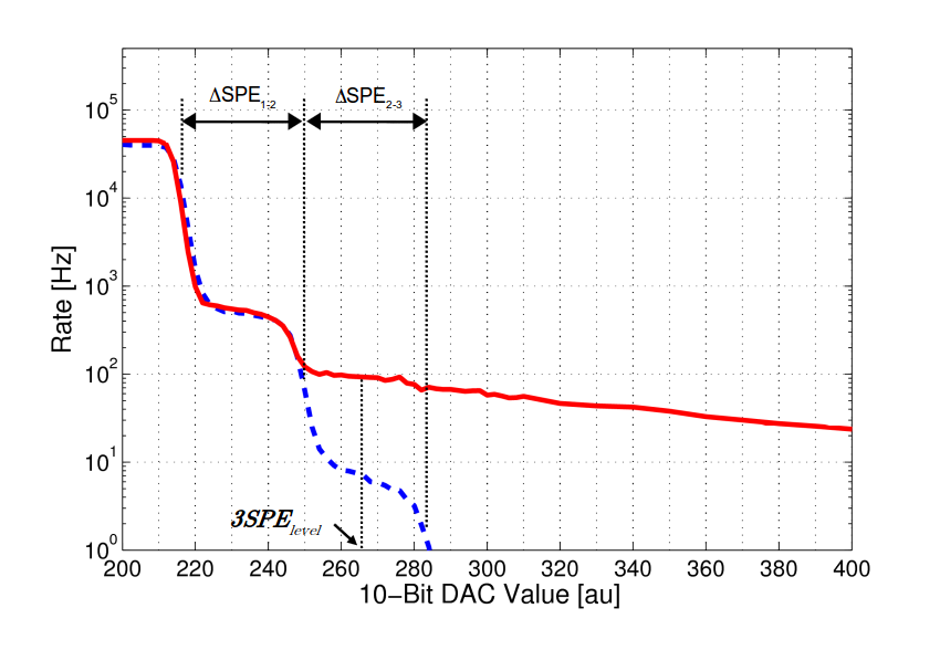
Figure 7: Measurement of the SiPM pulse rate with (red complete line) and without (blue dashed line) the scintillating bar over the 10-bit DAC value. Each plateau represents the transition for different amounts of SPEs. The value marked with the $3SPE_{level}$ is the selected value for the threshold of the discriminator. All the measurements were done at 25 ^∘C and $\Delta V=3.75\,V$.

As it was mentioned in subsection 4.1.2, the transition between plateaus in the SiPM rate as a function of the 10-bit DAC value represents the threshold of the comparator passing through the SPE peaks. Furthermore, as was mentioned in section 2, the amplitude of the signal generated by multiple simultaneously fired cells is directly proportional to the number of them. Therefore, it is expected that: $\Delta SPE_{1-2}=\Delta SPE_{2-3}=SPE_{peak}$ (see figure 7). In the example shown, the obtained values were: $\Delta SPE_{1-2}=(32.0\pm 1.4);\ \Delta SPE_{2-3}=(36.0\pm 1.4);\ SPE_{peak}=(34.0\pm 1.4)$ (in arbitrary units).

The middle point of the transition from the second to the third SPE peaks ($SPE_{peak}\ast 2.5$) corresponds to the value that ensures the detection of signals with three or more SPEs ($3SPE_{level}$). Considering the offset ($DC_{level}$), this value can be calculated with the following equation:

$$\begin{split}3SPE_{level}&=SPE_{peak}\ast 2.5+DC_{level}\simeq((216.0\pm 1.0)-(182.0\pm 1.0))\ast 2.5+(182.0\pm 1.0)\\ &=(216.0\pm 1.0)\ast 2.5-(182.0\pm 1.0)\ast 1.5=267.0\pm 2.9\end{split}$$ (4.6)

As an example, in the case exemplified in figure 7 the estimated $SPE_{peak}$ was $(34.0\pm 1.4)$ and the $DC_{level}$ was $(182.0\pm 1.0)$. The calculated $3SPE_{level}$ value is indicated in the figure, and it corresponds to the middle point of the third SPE plateau. The $3SPE_{level}$ must be estimated and set individually for each channel.

To estimate the accidental counting probability ($P_{accidental-counting}$) three factors are taken into account: the segmentation or number of strips ($n$), the acquired event time window ($T_{event}$) and the noise rate ($R_{noise}$, i.e. the environmental radiation and dark rate). As an example, for the AMIGA modules the segmentation is of 64 channels, the acquired event time window is 3.2 $\mu$s and the noise rate in the underground laboratory is $\sim$100 Hz (this value is the rate corresponding to $3SPE_{level}$ in figure 7). With those values, the accidental counting probability for a 10 m² module was estimated to be:

$$P_{accidental-counting}=n\cdot T_{event}\cdot R_{noise}\simeq 64\cdot 3.2\,\mu s\cdot 100\,Hz\equiv 2\,\%$$ (4.7)

which is below the desired level of 5 %. The efficiency will be studied in detail in section 5.

4.3 Proposed On-site Calibration

The electronics design enables calibration to be performed at the observatory site. To ensure its long-term performance, both calibrations detailed in sections 4.1 and 4.2 will be applied regularly and automatically. Each module will acquire the calibration data locally and then transmit it to a dedicated calibration server that will be running in the Central Data Acquisition System (CDAS) of the Pierre Auger Observatory. The calibration server will carry out the SiPM calibration as well as the detector calibration. This dedicated server will do the calculations to set three groups of parameters: the HV value, the 8-bit DAC to equalize the channels, and the 10-bit DAC value to set the discrimination level. All the calibration data and the parameters obtained will be stored for long-term stability studies.

5 Counting Efficiency Measurements

As mentioned in section 1, the module must count efficiently the number of impinging muons. To test its efficiency, the setup described in subsection 4.2.1 was used. Several measurements at different fiber lengths were taken using the muon telescope. Every time there is a muon telescope trigger (event), the acquisition system (see sixth stage of section 4.2.1) stores the discriminated signal of the CITIROC (digital trace) and the amplified analog signal of the SiPM (analog trace).

From the amplified analog traces, the voltage amplitude peak and charge (integral of the current) of each pulse were obtained by an offline analysis. The charge was numerically calculated integrating the voltage signal trace, in a time window of 200 ns, divided by the oscilloscope input impedance value (50 $\Omega$). A histogram illustrating the voltage amplitude peak and charge of the analog traces obtained at a fiber distance of 430 cm with the S13081-050CS SiPM is shown in figure 8. Two colored areas can be distinguished in each histogram. The red area represents the events that do not have a corresponding positive digital trace of the CITIROC. This means that no particle was detected by the counting system. The green area represents all the events that have a positive digital trace.

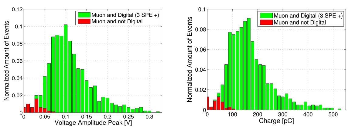
Figure 8: In the left (right) plot, the voltage amplitude peak (charge) histogram of 1000 triggered muon events is shown. The red colored area corresponds to the events that do not have a positive digital trace. All the measurements were done at 25 ^∘C, $\Delta V=3.75\,V$, and with the muon telescope placed at 430 cm of fiber from the SiPM.

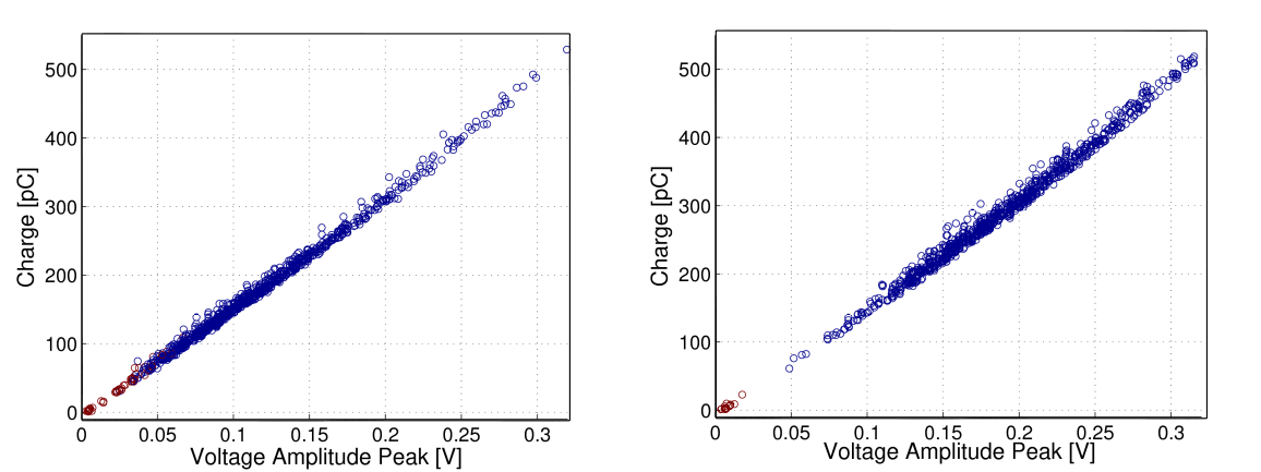
Figure 9: Both plots show the relationship between the voltage amplitude peak and the charge of 1000 triggered muon events. The red colored points correspond to events that do not have a digital output. In the left (right) plot the muon telescope was placed at 430 cm (130 cm) of fiber. Isolated red points in the lower left corner in the right figure evidence the false coincidences of the muon telescope trigger. All the measurements were done at 25 ^∘C and $\Delta V=3.75\,V$.

Both plots in figure 9 show a correlation between the voltage amplitude peak and charge of SiPM signals. In these plots there is a discrimination between the traces with (blue) or without (red) digital output. In the left plot, the results with the muon telescope placed at 430 cm of fiber are shown, and in the right one, the muon telescope was moved to 130 cm. As expected, the data sets have higher mean voltage amplitude and charge values due to a decrease in the light attenuation of the fiber.

In figure 10, the full width at half maximum (FWHM) of the digital output pulse of the CITIROC, acquired with the oscilloscope at two fiber distances measured is shown. As it was pointed out in the requirements, $99\,\%$ of the digital widths are lower than 35 ns. This requirement was achieved by the fast shaper included in the CITIROC. There was no evidence of afterpulses in the observed digital output.

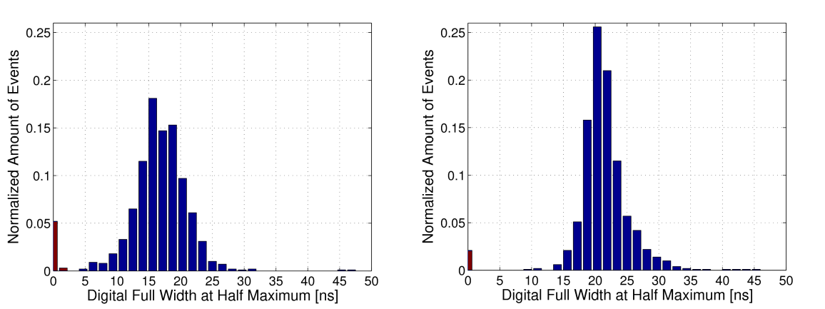
Figure 10: Both plots show the width histogram of 1000 digital output pulses of the CITIROC. The red colored bar corresponds to the traces that do not have a digital output pulse. In the left (right) plot the muon telescope was placed at 430 cm (130 cm) of fiber. All the measurements were done at 25 ^∘C and $\Delta V=3.75\,V$.

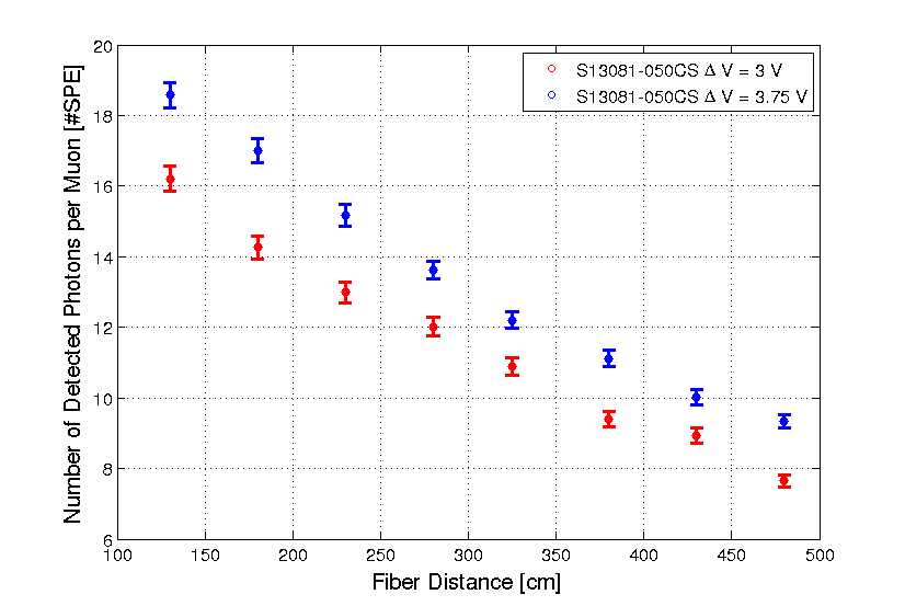
Figure 11: Number of detected photons per muon impinging the detector as a function of the fiber distance for two different overvoltages: $\Delta V=3\,V$ and $\Delta V=3.75\,V$. The detector light yield is not uniform due to the fiber attenuation. Error bars are only due to statistic errors of the mean. All the measurements were done at 25 ^∘C.

In figure 11, the mean value of the number of detected photons per muon impinging the detector as a function of the fiber distance is shown. This mean value was obtained as the mean value of the distribution of the ratio between the charge of measured traces and the mean charge of the SPE. Error bars are only due to statistic errors of the mean. This light yield curve was obtained with the setup shown in Figure 6. The muon telescope trigger selects mainly vertical muons and the acceptance angle considering the muon telescope geometry is $\rm\sim 35\,^{\circ}$. There are two main factors that constrain the performance of the detector since its light yield is not uniform due to the fiber attenuation. In the farther distances, the efficiency strongly depends on the threshold selection, since the attenuation of the optical fiber significantly decreases the number of photons that arrive to the SiPM. At the closest distances, the number of detected photons is higher and the digital width is consequently increased. The selected pre-amplifier gain, i.e. high-gain pre-amplifier set to the lowest gain, combined with the fast shaper ensures an adequate width of the digital output.

5.1 Efficiency Results and Possible Improvements

The counting efficiency is defined as the ratio between the amount of positive digital output traces of the CITIROC, and the number of triggers of the muon telescope that ensures a particle passing through the scintillating bar at a certain distance.

Figure 12 summarizes the results of the efficiency for eight different distances and for two different overvoltages. Two kind of errors are included in the plot. Vertical lines represent statistic errors assuming a binomial distribution and brackets represent the systematic errors caused by false triggers. It should be pointed out that the efficiency study was performed with the setup shown in Figure 6. The muon telescope trigger selects mainly vertical muons, the acceptance angle considering the muon telescope geometry is $\rm\sim 35\,^{\circ}$.

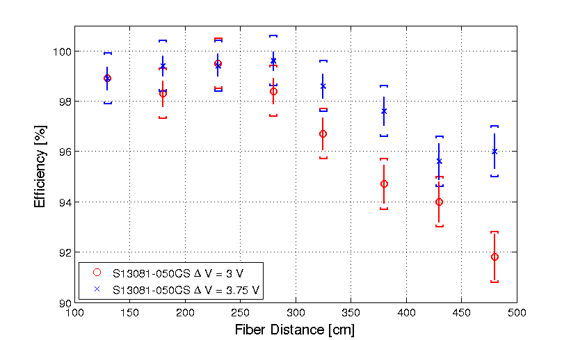
Figure 12: Efficiency measurements for two different $\Delta V$ are compared. A larger $\Delta V$ produces an increase in the efficiency. The estimated integrated efficiency is: 97 % for $\Delta V=3\,V$ (red) and 98 % for $\Delta V=3.75\,V$ (blue). Vertical lines represent statistic errors assuming a binomial distribution and brackets represent the systematics errors caused by false triggers.

A higher efficiency is achieved when the $\Delta V$ is increased, since the PDE of the SiPM rises with the increment of the $\Delta V$. With the increment of the $\Delta V$, the noise is also increased. For the higher $\Delta V$, the accidental counting probability is $\sim$2 % (see section 4.2.2).

Although the efficiency has a dependence with the distance, one important parameter that should be calculated is the integrated efficiency over the whole scintillating bar. For the two cases exemplified in figure 12, the estimated integrated efficiency is: 97 % for $\Delta V=3\,V$ and 98 % for $\Delta V=3.75\,V$.

6 Conclusions

A new readout for the AMIGA muon counters was proposed. The selected SiPM was the S13081-050CS due to its low crosstalk and afterpulsing. The CITIROC ASIC was selected as the electronics front-end. Its fast shaper enables a digital output width of the discriminator similar to the characteristic time width of the light pulses produced by the impinging particles in the detector. The Hamamatsu C11204-01 power supply was chosen for the biasing of the SiPMs.

The proposed calibration method consists of two steps. Firstly, the SiPM calibration allows the individual characterization of each SiPM of the module and the equalization between channels. Secondly, the detector calibration determines the discrimination level and the counting strategy. Both calibrations combined guarantee the performance of the detector by an adequate overvoltage and threshold level selection. Both methods were designed to be performed on the Observatory site. This allows studying the long-term performance of the detector, improving its stability for long periods.

Laboratory efficiency studies show promising results. The high integrated efficiency obtained (98 % for the higher tested overvoltage) combined with a low probability of accidental counting ($\sim$2 %) evidences an adequate performance of the proposed counting system.

The Pierre Auger Collaboration

A. Aab³⁷, P. Abreu⁶⁹, M. Aglietta^47,46, E.J. Ahn⁸⁴, I. Al Samarai²⁹, I.F.M. Albuquerque¹⁶, I. Allekotte¹, P. Allison⁸⁹, A. Almela^8,11, J. Alvarez Castillo⁶¹, J. Alvarez-Muñiz⁷⁹, M. Ambrosio⁴⁴, G.A. Anastasi⁴¹, L. Anchordoqui⁸³, B. Andrada⁸, S. Andringa⁶⁹, C. Aramo⁴⁴, F. Arqueros⁷⁶, N. Arsene⁷², H. Asorey^1,24, P. Assis⁶⁹, J. Aublin²⁹, G. Avila^9,10, A.M. Badescu⁷³, A. Balaceanu⁷⁰, C. Baus³², J.J. Beatty⁸⁹, K.H. Becker³¹, J.A. Bellido¹², C. Berat³⁰, M.E. Bertaina^55,46, X. Bertou¹, P.L. Biermann^b, P. Billoir²⁹, J. Biteau²⁸, S.G. Blaess¹², A. Blanco⁶⁹, J. Blazek²⁵, C. Bleve^49,42, M. Boháčová²⁵, D. Boncioli^39,d, C. Bonifazi²², N. Borodai⁶⁶, A.M. Botti^8,33, J. Brack⁸², I. Brancus⁷⁰, T. Bretz³⁵, A. Bridgeman³³, F.L. Briechle³⁵, P. Buchholz³⁷, A. Bueno⁷⁸, S. Buitink⁶², M. Buscemi^51,40, K.S. Caballero-Mora⁵⁹, B. Caccianiga⁴³, L. Caccianiga²⁹, A. Cancio^11,8, F. Canfora⁶², L. Caramete⁷¹, R. Caruso^51,40, A. Castellina^47,46, G. Cataldi⁴², L. Cazon⁶⁹, R. Cester^55,46, A.G. Chavez⁶⁰, A. Chiavassa^55,46, J.A. Chinellato¹⁷, J. Chudoba²⁵, R.W. Clay¹², R. Colalillo^53,44, A. Coleman⁹⁰, L. Collica⁴⁶, M.R. Coluccia^49,42, R. Conceição⁶⁹, F. Contreras^9,10, M.J. Cooper¹², S. Coutu⁹⁰, C.E. Covault⁸⁰, J. Cronin⁹¹, R. Dallier^e, S. D’Amico^48,42, B. Daniel¹⁷, S. Dasso^5,3, K. Daumiller³³, B.R. Dawson¹², R.M. de Almeida²³, S.J. de Jong^62,64, G. De Mauro⁶², J.R.T. de Mello Neto²², I. De Mitri^49,42, J. de Oliveira²³, V. de Souza¹⁵, J. Debatin³³, L. del Peral⁷⁷, O. Deligny²⁸, C. Di Giulio^54,45, A. Di Matteo^50,41, M.L. Díaz Castro¹⁷, F. Diogo⁶⁹, C. Dobrigkeit¹⁷, J.C. D’Olivo⁶¹, A. Dorofeev⁸², R.C. dos Anjos²¹, M.T. Dova⁴, A. Dundovic³⁶, J. Ebr²⁵, R. Engel³³, M. Erdmann³⁵, M. Erfani³⁷, C.O. Escobar^84,17, J. Espadanal⁶⁹, A. Etchegoyen^8,11, H. Falcke^62,65,64, K. Fang⁹¹, G. Farrar⁸⁷, A.C. Fauth¹⁷, N. Fazzini⁸⁴, B. Fick⁸⁶, J.M. Figueira⁸, A. Filevich⁸, A. Filipčič^74,75, O. Fratu⁷³, M.M. Freire⁶, T. Fujii⁹¹, A. Fuster^8,11, B. García⁷, D. Garcia-Pinto⁷⁶, F. Gaté^e, H. Gemmeke³⁴, A. Gherghel-Lascu⁷⁰, P.L. Ghia²⁹, U. Giaccari²², M. Giammarchi⁴³, M. Giller⁶⁷, D. Głas⁶⁸, C. Glaser³⁵, H. Glass⁸⁴, G. Golup¹, M. Gómez Berisso¹, P.F. Gómez Vitale^9,10, N. González^8,33, B. Gookin⁸², J. Gordon⁸⁹, A. Gorgi^47,46, P. Gorham⁹², P. Gouffon¹⁶, A.F. Grillo³⁹, T.D. Grubb¹², F. Guarino^53,44, G.P. Guedes¹⁸, M.R. Hampel^8,11, P. Hansen⁴, D. Harari¹, T.A. Harrison¹², J.L. Harton⁸², Q. Hasankiadeh⁶³, A. Haungs³³, T. Hebbeker³⁵, D. Heck³³, P. Heimann³⁷, A.E. Herve³², G.C. Hill¹², C. Hojvat⁸⁴, E. Holt^33,8, P. Homola⁶⁶, J.R. Hörandel^62,64, P. Horvath²⁶, M. Hrabovský²⁶, T. Huege³³, J. Hulsman^8,33, A. Insolia^51,40, P.G. Isar⁷¹, I. Jandt³¹, S. Jansen^62,64, J.A. Johnsen⁸¹, M. Josebachuili⁸, A. Kääpä³¹, O. Kambeitz³², K.H. Kampert³¹, P. Kasper⁸⁴, I. Katkov³², B. Keilhauer³³, E. Kemp¹⁷, R.M. Kieckhafer⁸⁶, H.O. Klages³³, M. Kleifges³⁴, J. Kleinfeller⁹, R. Krause³⁵, N. Krohm³¹, D. Kuempel³⁵, G. Kukec Mezek⁷⁵, N. Kunka³⁴, A. Kuotb Awad³³, D. LaHurd⁸⁰, L. Latronico⁴⁶, M. Lauscher³⁵, P. Lautridou, P. Lebrun⁸⁴, R. Legumina⁶⁷, M.A. Leigui de Oliveira²⁰, A. Letessier-Selvon²⁹, I. Lhenry-Yvon²⁸, K. Link³², L. Lopes⁶⁹, R. López⁵⁶, A. López Casado⁷⁹, Q. Luce²⁸, A. Lucero^8,11, M. Malacari¹², M. Mallamaci^52,43, D. Mandat²⁵, P. Mantsch⁸⁴, A.G. Mariazzi⁴, I.C. Mariş⁷⁸, G. Marsella^49,42, D. Martello^49,42, H. Martinez⁵⁷, O. Martínez Bravo⁵⁶, J.J. Masías Meza³, H.J. Mathes³³, S. Mathys³¹, J. Matthews⁸⁵, J.A.J. Matthews⁹⁴, G. Matthiae^54,45, E. Mayotte³¹, P.O. Mazur⁸⁴, C. Medina⁸¹, G. Medina-Tanco⁶¹, D. Melo⁸, A. Menshikov³⁴, S. Messina⁶³, M.I. Micheletti⁶, L. Middendorf³⁵, I.A. Minaya⁷⁶, L. Miramonti^52,43, B. Mitrica⁷⁰, D. Mockler³², L. Molina-Bueno⁷⁸, S. Mollerach¹, F. Montanet³⁰, C. Morello^47,46, M. Mostafá⁹⁰, G. Müller³⁵, M.A. Muller^17,19, S. Müller^33,8, I. Naranjo¹, S. Navas⁷⁸, L. Nellen⁶¹, J. Neuser³¹, P.H. Nguyen¹², M. Niculescu-Oglinzanu⁷⁰, M. Niechciol³⁷, L. Niemietz³¹, T. Niggemann³⁵, D. Nitz⁸⁶, D. Nosek²⁷, V. Novotny²⁷, H. Nožka²⁶, L.A. Núñez²⁴, L. Ochilo³⁷, F. Oikonomou⁹⁰, A. Olinto⁹¹, D. Pakk Selmi-Dei¹⁷, M. Palatka²⁵, J. Pallotta², P. Papenbreer³¹, G. Parente⁷⁹, A. Parra⁵⁶, T. Paul^88,83, M. Pech²⁵, F. Pedreira⁷⁹, J. Pȩkala⁶⁶, R. Pelayo⁵⁸, J. Peña-Rodriguez²⁴, L. A. S. Pereira¹⁷, L. Perrone^49,42, C. Peters³⁵, S. Petrera^50,41, J. Phuntsok⁹⁰, R. Piegaia³, T. Pierog³³, P. Pieroni³, M. Pimenta⁶⁹, V. Pirronello^51,40, M. Platino⁸, M. Plum³⁵, C. Porowski⁶⁶, R.R. Prado¹⁵, P. Privitera⁹¹, M. Prouza²⁵, E.J. Quel², S. Querchfeld³¹, S. Quinn⁸⁰, R. Ramos-Pollant²⁴, J. Rautenberg³¹, O. Ravel, D. Ravignani⁸, D. Reinert³⁵, B. Revenu^e, J. Ridky²⁵, M. Risse³⁷, P. Ristori², V. Rizi^50,41, W. Rodrigues de Carvalho⁷⁹, G. Rodriguez Fernandez^54,45, J. Rodriguez Rojo⁹, M.D. Rodríguez-Frías⁷⁷, D. Rogozin³³, J. Rosado⁷⁶, M. Roth³³, E. Roulet¹, A.C. Rovero⁵, S.J. Saffi¹², A. Saftoiu⁷⁰, H. Salazar⁵⁶, A. Saleh⁷⁵, F. Salesa Greus⁹⁰, G. Salina⁴⁵, J.D. Sanabria Gomez²⁴, F. Sánchez⁸, P. Sanchez-Lucas⁷⁸, E.M. Santos¹⁶, E. Santos⁸, F. Sarazin⁸¹, B. Sarkar³¹, R. Sarmento⁶⁹, C. Sarmiento-Cano⁸, R. Sato⁹, C. Scarso⁹, M. Schauer³¹, V. Scherini^49,42, H. Schieler³³, D. Schmidt^33,8, O. Scholten^63,c, P. Schovánek²⁵, F.G. Schröder³³, A. Schulz³³, J. Schulz⁶², J. Schumacher³⁵, S.J. Sciutto⁴, A. Segreto^38,40, M. Settimo²⁹, A. Shadkam⁸⁵, R.C. Shellard¹³, G. Sigl³⁶, G. Silli^8,33, O. Sima⁷², A. Śmiałkowski⁶⁷, R. Šmída³³, G.R. Snow⁹³, P. Sommers⁹⁰, S. Sonntag³⁷, J. Sorokin¹², R. Squartini⁹, D. Stanca⁷⁰, S. Stanič⁷⁵, J. Stasielak⁶⁶, F. Strafella^49,42, F. Suarez^8,11, M. Suarez Durán²⁴, T. Sudholz¹², T. Suomijärvi²⁸, A.D. Supanitsky⁵, M.S. Sutherland⁸⁹, J. Swain⁸⁸, Z. Szadkowski⁶⁸, O.A. Taborda¹, A. Tapia⁸, A. Tepe³⁷, V.M. Theodoro¹⁷, C. Timmermans^64,62, C.J. Todero Peixoto¹⁴, L. Tomankova³³, B. Tomé⁶⁹, A. Tonachini^55,46, G. Torralba Elipe⁷⁹, D. Torres Machado²², M. Torri⁵², P. Travnicek²⁵, M. Trini⁷⁵, R. Ulrich³³, M. Unger^87,33, M. Urban³⁵, A. Valbuena-Delgado²⁴, J.F. Valdés Galicia⁶¹, I. Valiño⁷⁹, L. Valore^53,44, G. van Aar⁶², P. van Bodegom¹², A.M. van den Berg⁶³, A. van Vliet⁶², E. Varela⁵⁶, B. Vargas Cárdenas⁶¹, G. Varner⁹², J.R. Vázquez⁷⁶, R.A. Vázquez⁷⁹, D. Veberič³³, V. Verzi⁴⁵, J. Vicha²⁵, L. Villaseñor⁶⁰, S. Vorobiov⁷⁵, H. Wahlberg⁴, O. Wainberg^8,11, D. Walz³⁵, A.A. Watson^a, M. Weber³⁴, A. Weindl³³, L. Wiencke⁸¹, H. Wilczyński⁶⁶, T. Winchen³¹, D. Wittkowski³¹, B. Wundheiler⁸, S. Wykes⁶², L. Yang⁷⁵, D. Yelos^11,8, A. Yushkov⁸, E. Zas⁷⁹, D. Zavrtanik^75,74, M. Zavrtanik^74,75, A. Zepeda⁵⁷, B. Zimmermann³⁴, M. Ziolkowski³⁷, Z. Zong²⁸, F. Zuccarello^51,40

¹

Centro Atómico Bariloche and Instituto Balseiro (CNEA-UNCuyo-CONICET), Argentina

²

Centro de Investigaciones en Láseres y Aplicaciones, CITEDEF and CONICET, Argentina

³

Departamento de Física and Departamento de Ciencias de la Atmósfera y los Océanos, FCEyN, Universidad de Buenos Aires, Argentina

⁴

IFLP, Universidad Nacional de La Plata and CONICET, Argentina

⁵

Instituto de Astronomía y Física del Espacio (IAFE, CONICET-UBA), Argentina

⁶

Instituto de Física de Rosario (IFIR) – CONICET/U.N.R. and Facultad de Ciencias Bioquímicas y Farmacéuticas U.N.R., Argentina

⁷

Instituto de Tecnologías en Detección y Astropartículas (CNEA, CONICET, UNSAM) and Universidad Tecnológica Nacional – Facultad Regional Mendoza (CONICET/CNEA), Argentina

⁸

Instituto de Tecnologías en Detección y Astropartículas (CNEA, CONICET, UNSAM), Centro Atómico Constituyentes, Comisión Nacional de Energía Atómica, Argentina

⁹

Observatorio Pierre Auger, Argentina

¹⁰

Observatorio Pierre Auger and Comisión Nacional de Energía Atómica, Argentina

¹¹

Universidad Tecnológica Nacional – Facultad Regional Buenos Aires, Argentina

¹²

University of Adelaide, Australia

¹³

Centro Brasileiro de Pesquisas Fisicas (CBPF), Brazil

¹⁴

Universidade de São Paulo, Escola de Engenharia de Lorena, Brazil

¹⁵

Universidade de São Paulo, Inst. de Física de São Carlos, São Carlos, Brazil

¹⁶

Universidade de São Paulo, Inst. de Física, São Paulo, Brazil

¹⁷

Universidade Estadual de Campinas (UNICAMP), Brazil

¹⁸

Universidade Estadual de Feira de Santana (UEFS), Brazil

¹⁹

Universidade Federal de Pelotas, Brazil

²⁰

Universidade Federal do ABC (UFABC), Brazil

²¹

Universidade Federal do Paraná, Setor Palotina, Brazil

²²

Universidade Federal do Rio de Janeiro (UFRJ), Instituto de Física, Brazil

²³

Universidade Federal Fluminense, Brazil

²⁴

Universidad Industrial de Santander, Colombia

²⁵

Institute of Physics (FZU) of the Academy of Sciences of the Czech Republic, Czech Republic

²⁶

Palacky University, RCPTM, Czech Republic

²⁷

University Prague, Institute of Particle and Nuclear Physics, Czech Republic

²⁸

Institut de Physique Nucléaire d’Orsay (IPNO), Université Paris 11, CNRS-IN2P3, France

²⁹

Laboratoire de Physique Nucléaire et de Hautes Energies (LPNHE), Universités Paris 6 et Paris 7, CNRS-IN2P3, France

³⁰

Laboratoire de Physique Subatomique et de Cosmologie (LPSC), Université Grenoble-Alpes, CNRS/IN2P3, France

³¹

Bergische Universität Wuppertal, Department of Physics, Germany

³²

Karlsruhe Institute of Technology, Institut für Experimentelle Kernphysik (IEKP), Germany

³³

Karlsruhe Institute of Technology, Institut für Kernphysik (IKP), Germany

³⁴

Karlsruhe Institute of Technology, Institut für Prozessdatenverarbeitung und Elektronik (IPE), Germany

³⁵

RWTH Aachen University, III. Physikalisches Institut A, Germany

³⁶

Universität Hamburg, II. Institut für Theoretische Physik, Germany

³⁷

Universität Siegen, Fachbereich 7 Physik – Experimentelle Teilchenphysik, Germany

³⁸

INAF – Istituto di Astrofisica Spaziale e Fisica Cosmica di Palermo, Italy

³⁹

INFN Laboratori del Gran Sasso, Italy

⁴⁰

INFN, Sezione di Catania, Italy

⁴¹

INFN, Sezione di L’Aquila, Italy

⁴²

INFN, Sezione di Lecce, Italy

⁴³

INFN, Sezione di Milano, Italy

⁴⁴

INFN, Sezione di Napoli, Italy

⁴⁵

INFN, Sezione di Roma “Tor Vergata“, Italy

⁴⁶

INFN, Sezione di Torino, Italy

⁴⁷

Osservatorio Astrofisico di Torino (INAF), Torino, Italy

⁴⁸

Università del Salento, Dipartimento di Ingegneria, Italy

⁴⁹

Università del Salento, Dipartimento di Matematica e Fisica “E. De Giorgi”, Italy

⁵⁰

Università dell’Aquila, Dipartimento di Chimica e Fisica, Italy

⁵¹

Università di Catania, Dipartimento di Fisica e Astronomia, Italy

⁵²

Università di Milano, Dipartimento di Fisica, Italy

⁵³

Università di Napoli “Federico II“, Dipartimento di Fisica “Ettore Pancini“, Italy

⁵⁴

Università di Roma “Tor Vergata”, Dipartimento di Fisica, Italy

⁵⁵

Università Torino, Dipartimento di Fisica, Italy

⁵⁶

Benemérita Universidad Autónoma de Puebla (BUAP), México

⁵⁷

Centro de Investigación y de Estudios Avanzados del IPN (CINVESTAV), México

⁵⁸

Unidad Profesional Interdisciplinaria en Ingeniería y Tecnologías Avanzadas del Instituto Politécnico Nacional (UPIITA-IPN), México

⁵⁹

Universidad Autónoma de Chiapas, México

⁶⁰

Universidad Michoacana de San Nicolás de Hidalgo, México

⁶¹

Universidad Nacional Autónoma de México, México

⁶²

Institute for Mathematics, Astrophysics and Particle Physics (IMAPP), Radboud Universiteit, Nijmegen, Netherlands

⁶³

KVI – Center for Advanced Radiation Technology, University of Groningen, Netherlands

⁶⁴

Nationaal Instituut voor Kernfysica en Hoge Energie Fysica (NIKHEF), Netherlands

⁶⁵

Stichting Astronomisch Onderzoek in Nederland (ASTRON), Dwingeloo, Netherlands

⁶⁶

Institute of Nuclear Physics PAN, Poland

⁶⁷

University of Łódź, Faculty of Astrophysics, Poland

⁶⁸

University of Łódź, Faculty of High-Energy Astrophysics, Poland

⁶⁹

Laboratório de Instrumentação e Física Experimental de Partículas – LIP and Instituto Superior Técnico – IST, Universidade de Lisboa – UL, Portugal

⁷⁰

“Horia Hulubei” National Institute for Physics and Nuclear Engineering, Romania

⁷¹

Institute of Space Science, Romania

⁷²

University of Bucharest, Physics Department, Romania

⁷³

University Politehnica of Bucharest, Romania

⁷⁴

Experimental Particle Physics Department, J. Stefan Institute, Slovenia

⁷⁵

Laboratory for Astroparticle Physics, University of Nova Gorica, Slovenia

⁷⁶

Universidad Complutense de Madrid, Spain

⁷⁷

Universidad de Alcalá de Henares, Spain

⁷⁸

Universidad de Granada and C.A.F.P.E., Spain

⁷⁹

Universidad de Santiago de Compostela, Spain

⁸⁰

Case Western Reserve University, USA

⁸¹

Colorado School of Mines, USA

⁸²

Colorado State University, USA

⁸³

Department of Physics and Astronomy, Lehman College, City University of New York, USA

⁸⁴

Fermi National Accelerator Laboratory, USA

⁸⁵

Louisiana State University, USA

⁸⁶

Michigan Technological University, USA

⁸⁷

New York University, USA

⁸⁸

Northeastern University, USA

⁸⁹

Ohio State University, USA

⁹⁰

Pennsylvania State University, USA

⁹¹

University of Chicago, USA

⁹²

University of Hawaii, USA

⁹³

University of Nebraska, USA

⁹⁴

University of New Mexico, USA

—–

^a

School of Physics and Astronomy, University of Leeds, Leeds, United Kingdom

^b

Max-Planck-Institut für Radioastronomie, Bonn, Germany

^c

also at Vrije Universiteit Brussels, Brussels, Belgium

^d

now at Deutsches Elektronen-Synchrotron (DESY), Zeuthen, Germany

^e

SUBATECH, École des Mines de Nantes, CNRS-IN2P3, Université de Nantes

References

- [1] The Pierre Auger Collaboration, The Pierre Auger Cosmic Ray Observatory, NIM A 798 (2015) 172-213 [doi:10.1016/j.nima.2015.06.058].
- [2] I. Allekotte, A. F. Barbosa, P. Bauleo, C. Bonifazi, B. Civit, C. O. Escobar, B. García, G. Guedes, M. Gómez-Berisso, J. L. Harton, M. Healy, M. Kaducak, P. Mantsch, P. O. Mazur, C. Newman-Holmes, I. Pepe, I. Rodriguez-Cabo, H. Salazar, N. Smetniansky-De Grande, D. Warner, for the Pierre Auger Collaboration, The Surface Detector System of the Pierre Auger Observatory, NIM A 586 (2008) 409-420 [doi:10.1016/j.nima.2007.12.016].
- [3] The Pierre Auger Collaboration, The Fluorescence Detector of the Pierre Auger Observatory, NIM A 620 (2010) 227-251 [doi:10.1016/j.nima.2010.04.023].
- [4] A. Etchegoyen for the Pierre Auger Collaboration, AMIGA, Auger Muons and Infill for the Ground Array, Published as Proceedings of 30th ICRC, Mérida, México, 5 (2007) 1191-1194 [arXiv:0710.1646].
- [5] M. Platino for the Pierre Auger Collaboration, AMIGA, Auger Muons and Infill for the Ground Array of the Pierre Auger Observatory, Published as Proceedings of 31st ICRC, Łódź, Poland, 5 (2009) 14-17 [arXiv:0906.2354].
- [6] P. Buchholz for the Pierre Auger Collaboration, Hardware Developments for the AMIGA enhancement at the Pierre Auger Observatory, Published as Proceedings of 31st ICRC, Łódź, Poland, 5 (2009) 22-25 [arXiv:0906.2354].
- [7] The KASCADE Collaboration, The cosmic-ray experiment KASCADE, NIM A 513 (2003) 490-510 [doi:10.1016/S0168-9002(03)02076-X].
- [8] The KASCADE-Grande Collaboration, The KASCADE-Grande experiment, NIM A 620 (2010) 202-216 [doi:10.1016/j.nima.2010.03.147].
- [9] The Pierre Auger Collaboration, Prototype muon detectors for the AMIGA component of the Pierre Auger Observatory, JINST 11 (2016) P02012 [doi:10.1088/1748-0221/11/02/P02012].
- [10] S. Piatek, Hamamatsu Corporation & New Jersey Institute of Technology, Physics and Operation of an MPPC, (2014). 430
- [11] P. Eckert et al., Characterisation Studies of Silicon Photomultipliers, NIM A 620 (2010) 217-226 [doi:10.1016/j.nima.2010.03.169]
- [12] S. M. Sze and K. K. Ng, Physics of Semiconductor Devices, NJ: Wiley-Interscience (2007) [ISBN:978-0-471-14323-9]
- [13] A. D. Supanitsky, A. Etchegoyen, G. Medina-Tanco, I. Allekotte, M. Gómez Berisso, M. C. Medina, Underground Muon Counters as a Tool for Composition Analyses, Astroparticle Physics 29 (2008) 461-470 [doi:10.1016/j.astropartphys.2008.05.003].
- [14] B. Wundheiler for the Pierre Auger Collaboration, The AMIGA muon counters of the Pierre Auger Observatory: performance and first data, Published as Proceedings of 32nd ICRC, Beijing, China, (2011) #0341 [doi:10.1088/1742-6596/375/1/052006].
- [15] O. Wainberg et al., Digital electronics for the Pierre Auger Observatory AMIGA muon counters, JINST 9 (2014) T04003 [doi:10.1088/1748-0221/9/04/T04003].
- [16] A. Almela et al., Design and implementation of an embedded system for particle detectors, Published as Proceedings of 33rd ICRC, Rio de Janeiro, Brazil, (2013) #1209 [ISBN:978-85-89064-29-3].
- [17] Hamamatsu Photonics K.K., MPPC Multi-pixel photon counter, S12571-25, -50, -100C/P specification datasheet, (2015).
- [18] Hamamatsu Photonics K.K., MPPC Multi-pixel photon counter, S12572-25, -50, -100C/P specification datasheet, (2015).
- [19] Weeroc, CITIROC, (2014).
- [20] Hamamatsu Photonics K.K., Power supply for MPPC, (2015).
- [21] V. Chmill et al., Study of the breakdown voltage of SiPMs, Instrumentation and Detectors (physics.ins-det) (2016) 047 [doi:10.1016/j.nima.2016.04.047]
- [22] M. Platino et al., AMIGA at the Auger Observatory: the scintillator module testing system, JINST (2011) P06006 [doi:10.1088/1748-0221/6/06/P06006]
- [23] B. Wundheiler for the Pierre Auger Collaboration, The AMIGA muon counters of the Pierre Auger Observatory: Performance and Studies of the Lateral Distribution Function, Published as Proceedings of 34th ICRC, The Hague, The Netherlands, (2015) #0324 [arXiv:1509.03732].
- [24] D. Ravignani and A.D. Supanitsky, A new method for reconstructing the muon lateral distribution with an array of segmented counters, Astroparticle Physics 65 (2015) 1-10 [doi:10.1016/j.astropartphys.2014.11.007]