A Hitch-hiker’s Guide to Stochastic Differential Equations

Abstract

In this review, an overview of the recent history of stochastic differential equations (SDEs) in application to particle transport problems in space physics and astrophysics is given. The aim is to present a helpful working guide to the literature and at the same time introduce key principles of the SDE approach via “toy models”. Using these examples, we hope to provide an easy way for newcomers to the field to use such methods in their own research. Aspects covered are the solar modulation of cosmic rays, diffusive shock acceleration, galactic cosmic ray propagation and solar energetic particle transport. We believe that the SDE method, due to its simplicity and computational efficiency on modern computer architectures, will be of significant relevance in energetic particle studies in the years to come.

1 Introduction

Would it save you a lot of time if I just gave up and went mad now?

Adams (1979, h2g2)

Studying the transport of non-thermal particles through turbulent plasmas is ubiquitous in space and astrophysics. Examples include, amongst others, the propagation of cosmic rays through the galaxy and the heliosphere. The transport of these particles is usually described by a Fokker-Planck type diffusion equation that must, for most applications, be solved numerically due to the complexity of both the plasma geometry and the associated transport parameters. In recent years, stochastic differential equations (SDEs) have been used more frequently to numerically solve a variety of problems in space- and astrophysics. It appears that SDEs have, to some extent, replaced or at least complemented more traditional (i.e. largely finite difference (FD) type) numerical schemes to solve multi-dimensional partial differential equations (PDEs) which involve diffusive processes. As such, we have decided to compile this review, which consists of two parts or aspects: (i) Simple 1D “toy models” are constructed, discussed in detail, and used to illustrate how SDEs are solved numerically for a variety of different boundary conditions, how source/sink terms are handled numerically and how to deal with some numerical pitfalls that might exist (for example, how to select an appropriate time step). (ii) Directly after each numerical section, a review is given on some of the most relevant and contemporary SDE-based models that are currently available and implement the previously discussed numerical techniques for the solution of real-world problems. The primary aim of this paper is therefore to introduce SDE-type numerical techniques to novices in the field and to give a guide to the reader in applying these methods in his/her own work.

The scope of applications considered here can loosely be defined as energetic particle transport in space and astrophysical plasmas. The common modeling ground for corresponding transport processes is a Fokker-Planck type equation which involves both diffusive (i.e. stochastic or random) and convective (i.e. deterministic) processes. The limits of this approach can be understood in the kinetic behaviour of the particles: at low energies and sufficiently high densities the particles may thermalize, making a kinetic treatment superfluous. At very high energies and low densities, the particles may not scatter anymore with the background plasma fluctuations on the relevant length and time scales, and thus a completely deterministic treatment of the problem is possible, e.g. by solving the Newton-Lorentz equations of motion for individual particles (see also the discussions in Schlickeiser, 2002; Shalchi, 2009). We do not consider these two limits here and suppose that a Fokker-Planck like transport equation is always the proper starting point (see, e.g., Schlickeiser, 1989, for a classical derivation of the Fokker-Planck equation in the context of cosmic ray transport).

We begin by describing very briefly the mathematical background of the problem, before we consider different aspects of the modeling approach and practical computational issues in conjunction with selected applications. These are, in the order of the subsequent chapters: the solar modulation of cosmic rays, diffusive shock acceleration, galactic cosmic ray propagation and solar energetic particle transport.

And above all, we emphasize: Don’t Panic.

1.1 Mathematical background

Several monographs deal with the mathematical formalism related to SDEs and their application in a variety of scientific fields (e.g. Kloeden et al., 1994; Kloeden and Platen, 1999; Øksendal, 2003; Gardiner, 2009). For those completely new to the subject, we recommend the excellent introductory book by Lemons (2002). Also, the classical review by Chandrasekhar on stochastic problems (Chandrasekhar, 1943) needs to be mentioned. The discussion in this section is based on these sources. We only present the most relevant aspects for the purposes of this paper, without any attempt for strict mathematical rigor or derivations.

For our purposes, it is sufficient to define an SDE as any equation that can be cast into the general form

$$\frac{dx(t)}{dt}=a(x,t)+b(x,t)\zeta(t)$$ (1)

in the 1D case where $a(x,t)$ and $b(x,t)$ are continuous functions, while $\zeta(t)$ represents a rapidly varying stochastic function, also referred to as a noise term. In SDE nomenclature, the first term on the right-hand side of Eq. 1 is referred to as the drift or deterministic term, while the second is referred to as the diffusion term (not to be confused with the physical drift and diffusive processes that will be considered later on). Moreover, only SDEs of the $\mathrm{It\bar{o}}$ type are considered here, where Eq. 1 can be rewritten as

$$dx(t)=a(x,t)dt+b(x,t)dW(t)$$ (2)

with $W(t)$ representing the Wiener process; a time stationary stochastic Lévy process where the time increments have a Normal distribution with a mean of zero (i.e. a Gaussian distribution) and a variance of $dt$; $dW(t)=W(t+dt)-W(t)\sim\mathcal{N}(0,dt)$. In fact, the Wiener process can be understood as the integral of the stochastic function present in Eq. 1, i.e. in its differential form we have $dW(t)=\zeta(t)dt$. See especially the introduction by Gardiner (2009).

Eq. 2 can be integrated formally as

$$x(t)=x_{0}+\int_{0}^{t}a(x,t^{\prime})dt^{\prime}+\int_{0}^{t}b(x,t^{\prime})dW(t^{\prime})$$ (3)

where the first integral is a normal (Riemann or Lebesgue) integral, while the second is an $\mathrm{It\bar{o}}$-type stochastic integral. Analytical solutions for SDEs are, however, only available for very few limited scenarios (for an example, see the discussion of the Ornstein-Uhlenbeck process in Lemons, 2002), and as such, Eq. 3 is usually integrated numerically. In the most common approach, the SDEs are integrated by using the Euler-Maruyama numerical scheme (Maruyama, 1955), where a finite time step $\Delta t$, is chosen and Eq. 2 is solved iteratively

$$x(t+\Delta t)=x(t)+a(x,t)\Delta t+b(x,t)\Delta W(\Delta t)$$ (4)

from an initial position $x=x_{0}$ at $t=0$ and continued until either a boundary is reached at $x=x_{e}$ at $t=t_{e}$, or until a temporal integration limit is reached at $t=T$. Higher-order schemes (in time) are available (see, e.g., the book by Kloeden and Platen, 1999), but often the simple Euler time stepping is sufficient, particularly in diffusion-dominated cases. For a comparison of different higher-order numerical schemes, see also Wawrzynczak et al. (2015b).

By using $\mathcal{N}(0,dt)\stackrel{{\scriptstyle d}}{{=}}\mathcal{N}(0,1)\sqrt{dt}$ (where the symbol $\stackrel{{\scriptstyle d}}{{=}}$ indicates that the random processes follow the same distribution) it follows that the Wiener process can be discretized as

$$\Delta W(\Delta t)=\sqrt{\Delta t}\cdot\Lambda(t),$$ (5)

where $\Lambda(t)$ is a simulated Gaussian distributed pseudo-random number (PRN). The temporal evolution of $x$ forms a trajectory through phase space, which is generally referred to as the trajectory of a pseudo-particle (this is a widely used, but somewhat inappropriate term, that has become part of the nomenclature of the field; the actually meaning of the term is discussed in Sec. 2.5.3 where, for the case of charged particle propagation, we show that this pseudo-particle actually represents the temporal evolution of an ensemble of real particles, or equivalently, the evolution of a phase-space density element). Integrating Eq. 4 for a single pseudo-particle has no significance, as integration must be carried out over a large number of possible trajectories (i.e. over a large number of possible Wiener processes; see Eq. 3), so that Eq. 4 is usually integrated $N\gg 1$ times, each time using a different series of simulated Wiener processes, starting the integration process with different seeds to the pseudo random number generator (PRNG); this process is sometimes referred to as tracing $N$ pseudo-particles. Numerically, the independence of the pseudo-random numbers (PRNs; referring to the computational technique of simulating random numbers via deterministic algorithms) is a very important condition to fulfil in the numerical model, as some PRNGs are not independent and have a quite short cycling period (meaning the same set of PRNs are repeated after a certain time). A “high level” PRNG is therefore needed, e.g. the Mersenne Twister PRNG (Matsumoto and Nishimura, 1988). When SDEs are solved on parallel computing architectures, it is important that the PRNs, simulated on different compute cores, are also independent (e.g. Dunzlaff et al., 2015).

We can generalize Eq. 2 to an $n$-dimensional set of SDEs, so the general formulation becomes

$$dx_{i}=a_{i}(x_{i},s)ds+\sum_{j=1}^{n}b_{ij}(x_{i},s)dW_{i}(s),$$ (6)

where $\vec{a}$ is an $n$-dimensional vector and $\mathbf{b}$ is a $n\times n$ matrix. In general, this system of SDEs can be thought of as being integrated either backward or forward in time (more on the relative merits of each approach in the next section). When time backward integration is performed, Eq. 6 is equivalent to the following Fokker-Planck equation (also referred to as the time backward Kolmogorov equation)

$$-\frac{\partial\rho(x_{i},s)}{\partial s}=\sum_{i=1}^{n}a_{i}(x_{i},s)\frac{\partial\rho(x_{i},s)}{\partial x_{i}}+\frac{1}{2}\sum_{i=1}^{n}\sum_{j=1}^{n}C_{ij}(x_{i},s)\frac{\partial^{2}\rho(x_{i},s)}{\partial x_{i}\partial x_{j}},$$ (7)

where $\rho(x_{i},s)$ is a conditional probability density, depending on all $x_{i}$, $s$ and a final condition for $\rho$ at time $T$. Note that we introduced $s$ as a new time-marching coordinate to indicate that it can be different from actual (forward moving) time $t$ (the equivalence between time forward and time backward integration is discussed in more detail in Sec. 2).

If time forward integration is performed instead, the corresponding Fokker-Planck equation (also referred to as the time forward Kolmogorov equation in order to distinguish it from Eq. 7) is given by

$$\frac{\partial\rho(x_{i},t)}{\partial t}=-\sum_{i=1}^{n}\frac{\partial}{\partial x_{i}}\left[\tilde{a}_{i}(x_{i},t)\rho(x_{i},t)\right]+\frac{1}{2}\sum_{i=1}^{n}\sum_{j=1}^{n}\frac{\partial^{2}}{\partial x_{i}\partial x_{j}}\left[\tilde{C}_{ij}(x_{i},t)\rho(x_{i},t)\right].$$ (8)

Note that the main difference between both equations is the implicit vs. explicit formulation in the coefficients, which may then differ for the different formulations. For most cases, $\vec{a}\neq\tilde{\vec{a}}$ and $\vec{C}\neq\tilde{\vec{C}}$. We point to Kopp et al. (2012) and Bobik et al. (2016) for a detailed discussion on how the time forward and backward SDE formulation is related to different Fokker-Planck equations. Moreover, we note that the “full” Fokker-Planck equation can also contain source and linear terms, while are not included in Eqs. 7 and 8. These additional terms are however included in Secs. 4 and 5, respectively.

The diffusion tensor $C_{ij}$ is given by

$$C_{ij}(x_{i},s)\equiv\left(b_{ij}(x_{i},s)\cdot b_{ji}(x_{i},s)\right).$$ (9)

The quantity $b_{ij}$ is sometimes referred to as the volatility matrix (especially in mathematical texts), to illustrate that it is related to, but is not the same as the diffusion matrix (or tensor). A suitable Fokker-Planck like PDE can therefore be cast into the form of Eq. 7, the quantities $\vec{a}$ and $\mathbf{b}$ obtained, and the equivalent SDE formulation emerges naturally. The $n$-dimensional PDE is thereby transformed into a set of $n-1$ two-dimensional SDEs, with the latter usually much easier to solve numerically. In the remainder of this paper, we will be concerned with such solution methods and corresponding applications. It should be mentioned at this point that linear loss or gain and source terms can, of course, be of importance in many circumstances when Fokker-Planck type models are used. We will return to some of the issues related to the inclusion of such terms in the corresponding following sections.

1.2 Why should one use the time-backward method?

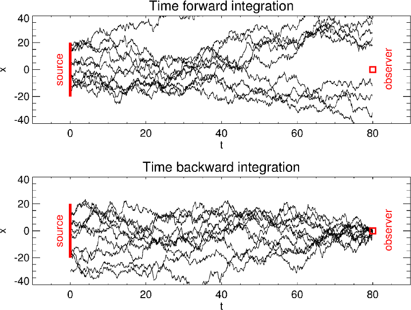
Figure 1: Illustrating time forward (top panel) and time backward (bottom panel) integration of SDEs in a 1D scenario.

In energetic particle transport applications of SDEs, the time backward integration approach is mostly followed. In Fig. 1, it is demonstrated why this is the case: The top panel shows, for illustration purposes, 10 solutions of a 1D SDE, as a function of time, starting at a “source” region (the thick red line at $t=0$). In most astrophysical and heliospheric applications, we are however only interested in calculating the solution of the PDE at a collection of phase-space points, which may be, for example, along the trajectory of a spacecraft or an energy spectrum at a given position. For the top panel of the figure, we are therefore interested in the intensity at an “observational point” (indicated by the red square at $t=80$). It is clear that for this set-up, none of the SDE solutions pass through the observational point, and hence, they do not contribute to the intensity at the observational point – these pseudo-particle trajectories were thus unnecessarily solved and simply wasted computational resources. A much more efficient set-up is illustrated in the bottom panel of the figure: Integration is started at the observational point (where one wants the solution) and traced (solved/integrated) backward in time until model boundaries are reached (for a comparison between the time forward and backward approaches, see Bobik et al., 2016). For many applications, the latter set-up is more efficient. In this review, we will thus focus almost solely on the backward integration method.

1.3 Advantages of the SDE method

There are numerous advantages to adopt an SDE-based numerical scheme above more traditional finite difference methods. These advantages include: (i) The SDE numerical scheme is unconditionally stable, although this does not necessarily imply numerical accuracy. (ii) Related to this, the method can handle large gradients, something that finite difference models struggle with, but care has to be taken in the choice of the time step (see Section 3). (iii) The SDE approach does not calculate solutions on a specific grid, but at a number of discrete phase-space positions. There is thus no need to store unnecessary information, saving computational memory and making computations in higher dimensions possible. (iv) Each solution (i.e. each pseudo-particle) is completely independent, making it possible to perform calculations on parallel computational environments, significantly speeding up calculations. Calculations can also performed in parallel on graphics processing units (GPUs, Dunzlaff et al., 2015). (v) The SDE approach allows one to visualize more of the physics (processes) included in the transport equation under investigation. This will be illustrated further in this work.

2 Handling Boundary Conditions: Solar Modulation of Cosmic Rays

For a moment, nothing happened. Then, after a second or so, nothing continued to happen.

h2g2

We start by considering a simple one-dimensional diffusion equation

$$\frac{\partial f(x,t)}{\partial t}=\kappa\frac{\partial^{2}f}{\partial x^{2}}$$ (10)

where $\kappa=1/2$ is assumed to be constant. This equation is solved on the interval $x\in[x_{\min},x_{\max}]=[-1,1]$. Referring to Eqs. 2 and 7, the time-backward SDE, being equivalent to Eq. 10, is

$$dx=bdW$$ (11)

with $b=1$. For this one-dimensional situation, $\vec{b}$, which is in the general case a tensor, reduces to a scalar. Similarly for the general tensor $\vec{C}$, where a comparison between Eqs. 7 and 10 show that, for this specific set-up, $C=2\kappa$.

In general, the solution at any point $x$, at any time $T$, can obtained by solving the convolution, (see e.g. Pei et al., 2010)

$$f(x,T)=\int_{0}^{T}\int_{x}G(x^{\prime},t)f_{b}(x^{\prime},t)dx^{\prime}dt$$ (12)

where $f_{b}(x^{\prime},t)$ denotes the boundary value for either Dirichlet-type or initial boundary conditions. Here Eq. $G(x,t)$ is a Green’s function of the considered PDE (e.g. Webb and Gleeson, 1977), where the normalization condition

$$\int_{0}^{\infty}\int_{-\infty}^{\infty}G(x^{\prime},t)dx^{\prime}dt=1.$$ (13)

holds.

For the scenarios considered in this section, $f_{b}(x,t)$ has the general form

$$f_{b}(x,t)=\underbrace{g(t)\delta(x+1)}_{\text{left boundary}}+\underbrace{h(t)\delta(x-1)}_{\text{right boundary}}+\underbrace{k(x)\delta(t)}_{\text{initial condition}}$$ (14)

where $g(t)$ and $h(t)$ are boundary conditions specified at $x=\pm 1$ respectively and $k(x)$ is an initial condition. Eq. 12 then becomes

$$f(x,T) = \underbrace{\int_{0}^{T}g(t)G(x=-1,t)dt}_{\text{left boundary contribution}}$$ (15)

$$+ \underbrace{\int_{0}^{T}h(t)G(x=1,t)dt}_{\text{right boundary contribution}}$$

$$+ \underbrace{\int_{-1}^{1}k(x)G(x,t=0)dx}_{\text{initial condition contribution}}.$$

The normalization condition of $G(x,t)$ of course still applies

$$\underbrace{\int_{0}^{\infty}G(x=-1,t)dt}_{\text{left boundary}}+\underbrace{\int_{0}^{\infty}G(x=1,t)dt}_{\text{right boundary}}+\underbrace{\int_{-1}^{1}G(x,t=0)dx}_{\text{initial condition}}=1$$ (16)

For the results presented here, time backward integration is performed, and the solution is only calculated at $x=0$ by means of the SDE model. Although, in this section, we calculate the solution only at a single $x$ point, extension of the scheme for different values of $x$ is simple and will be discussed in the following sections. The SDE results are compared to the solution from a finite difference numerical scheme in order to validate the numerical approach applied here.

Backward time $s$, is related to forward time $t$, via

$$s=T-t$$ (17)

where $T$ is our temporal boundary. Also note that, for example, $G(x,t=0)=G(x,s=T)$.

As we want the solution of the SDE at $x=0$, $N$ pseudo-particles are released from $x=0$ at $s=0$ (this implies $G(x,s)=\delta(x)\delta(s)$) and their stochastic trajectories are traced until the temporal boundary $s=T$ is reached. The trajectory of a small number ($N=5$) of such particles are shown in panel (g) of Fig. 2, where they are integrated from $s=0$ to $s=0.5$. At this point, $G(x,t)$ is calculated by binning the position of the pseudo-particles in either a spatial and/or temporal grid. For example, to apply the initial condition, the spatial grid is divided into $M$ equally spaced grid cells and the number of pseudo-particles in each cell, $N_{j}(x_{j},s)$, where $x_{j}$ refers to the mid-point of each spatial cell, at $s=T$ is recorded, or the pseudo-particles interact with the spatial boundaries, dividing by the total number of pseudo-particles injected initially, one may calculate

$$G(x_{j},t=0)dx\approx\frac{N_{j}}{N}.$$ (18)

From here it is easy to calculate

$$f^{\prime}(x,T)=\int_{-1}^{1}k(x)G(x,t=0)dx\approx\frac{1}{N}\sum_{j=1}^{M}k(x_{j})N_{j}$$ (19)

where $x_{j}$ is the spatial position of the $j$-th bin. $f^{\prime}(x,T)$ is the contribution of the initial condition to the value of $f(x,T)$. A similar approach is then also applied to the boundaries, although integration for this scenario is performed over time and not space. In a later section it will become clear how this binning process works and that, for some applications, the binning process is redundant so that the solution can be obtained directly from the exit position of the pseudo-particles.

2.1 Dirichlet Boundary Conditions

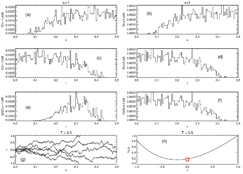
Figure 2: Calculating the solution of the PDE, given by Eq. 10, by means of a SDE numerical method for $(x=0,t=0.5)$. Panels (a) and (b) show the calculated probability distributions ($G(x=-1,s)$ and $G(x=1,s)$) for either the left or right boundaries, binned in terms of backward time. These are then converted to forward time and shown in panels (c) and (d), while the convolutions with the boundary conditions are shown in panels (e) and (f). The solution of the SDE approach is shown in panel (h) as the red box while the solid line is the solution of a FD scheme. For illustrative purposes, panel (g) shows the trajectory of 5 pseudo-particles.

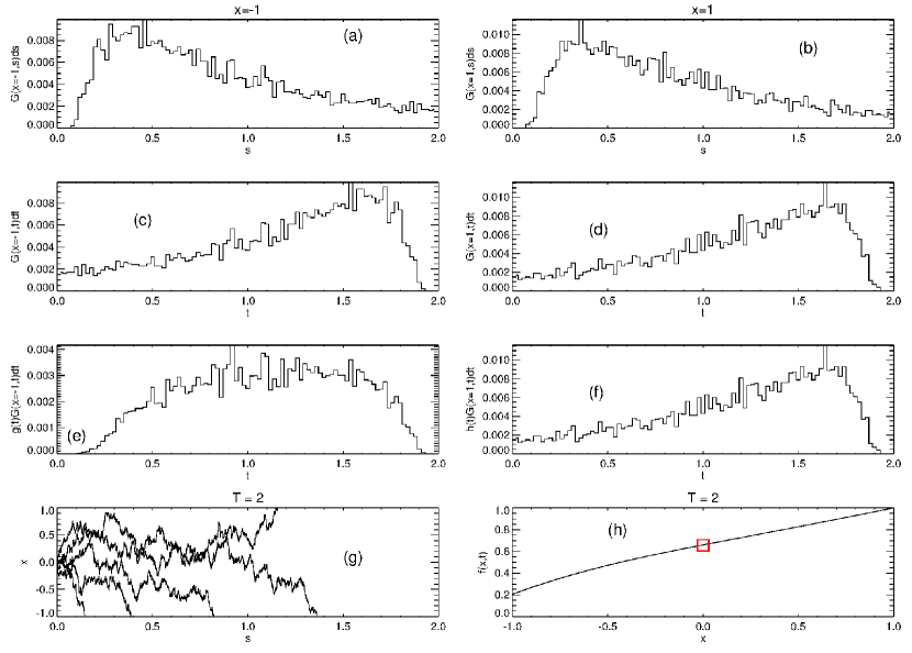
Figure 3: Similar to Fig. 2, but for $T=2$.

We first consider Eq. 10 for the case of $f(x,t=0)=0$ (an empty system as an initial condition, i.e. $k(x)=0$) and the following boundary conditions

$$g(t) = \frac{5}{t}\exp\left[-\frac{1}{t}-\frac{t}{1}\right]$$ (20)

$$h(t) = 1.$$ (21)

The complete methodology to calculate the solution at two different times, $f(x=0,t=0.5)$ and $f(x=0,t=2)$, is illustrated in Figs. 2 and 3. In Fig. 2, the different panels show the calculated $G(x,s)ds$ for $x=-1$ (panel a) and $x=1$ (panel b) for $T=0.5$. They are thus the binned (in terms of backward-time) normalized number of pseudo-particles reaching either the left or right boundary. These quantities are then converted to forward-time and shown as $G(x=-1,t)dt$ (panel c) and $G(x=1,t)dt$ (panel d). Note that for the discretized SDE formulation, all particles that exit the computational region are assumed to interact with the spatial boundaries, therefore all particles with e.g. $x\leq-1$ are counted in the calculation of $G(x=-1,t)dt$. The convolutions $g(t)G(x=-1,t)dt$ (panel e) and $h(t)G(x=1,t)dt$ (panel f) are shown for illustrative purposes, while the solution of the SDE scheme at $(x=0,t=0.5)$ is shown as the red box in panel (h). In this panel, the solid line shows the solution of the FD scheme. Panel (g) shows the trajectory of 5 pseudo-particles for illustrative purposes, all released from $x=0$ (the position at which we want the solution). The inversion $G(x,s)ds\rightarrow G(x,t)dt=G(x,T-s)ds$ is not really needed in calculations as the convolutions may be done directly in terms of backward time, e.g.

$$\int_{0}^{T}h(t)G(x,t)dt=\int_{T}^{0}h(T-s)G(x,s)ds,$$ (22)

but is shown here for completeness sake.

Interesting for the SDE scenario is that the steady-state solution is well defined (in contrast to FD scheme where convergence to a steady state must be checked continuously) for the time backward SDE formulation – it is simply when all the pseudo-particles have exited the computational domain, i.e.

$$t\rightarrow\infty\Rightarrow G(-1<x<1,t)dt\rightarrow 0.$$ (23)

Fig. 3 is similar to Fig. 2, but for a later time $T=2$.

2.2 Initial Conditions

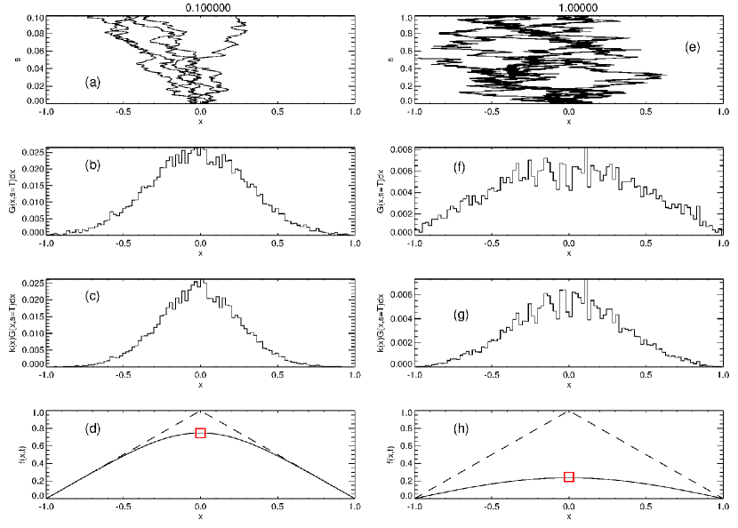
Figure 4: The calculation of $f(x=0,t)$ for $T=0.1$ (left panels) and $T=1$ (right panels). In the bottom panels, the red box shows the solution of the SDE approach, the solid line that of a FD scheme and the dashed line indicates the initial condition specified at $t=0$.

We now turn to the case of a prescribed initial condition. We choose $k(x)=-|x|+1$ along with absorbing boundary conditions at the spatial boundaries, i.e. $g(t)=h(t)=0$.

Fig. 4 shows the calculation of $f(x=0,t)$ for $T=0.1$ (left panels) and $T=1$ (right panels). Panels (a) and (e) again shows illustrative pseudo-particle trajectories, while panels (b) and (f) show $G(x,s=0.1)dx$ and $G(x,s=1)dx$. This time the pseudo-particles are binned in terms of spatial position at $s=T(t=0)$. The corresponding convolutions with the initial condition are shown in panels (c) and (g), while panels (d) and (h) again compare the final solution of the SDE approach to that of the FD scheme. The dashed line indicates the initial solution. For the SDE approach, the solution at $T=0\Rightarrow s,t=0$ is readily obtained: Keeping in mind that $G(x,t=0)dx=G(x,s=0)dx=\delta(x=0)\delta(t=0)$, the solution is simply $f(x,t=0)=k(x)$ as required.

2.3 Von Neumann Boundary Conditions

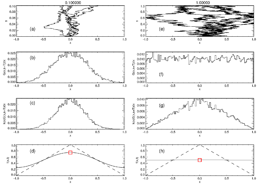
Figure 5: Similar to Fig. 4, except that reflecting boundary conditions are assumed at $x=\pm 1$.

The solutions presented here are similar to that of the previous section, except that reflecting conditions are assumed, where

$$\left.\frac{\partial f(x,t)}{\partial x}\right|_{x=\pm 1}=0.$$ (24)

Reflecting conditions are implemented in the SDE formulation as

$$x<x_{\min} : x\rightarrow-2x_{\mathrm{min}}-x=-2-x$$ (25)

$$x>x_{\max} : x\rightarrow 2x_{\mathrm{max}}-x=2-x$$ (26)

similarly to hard sphere reflection off a planar surface. Note that for this situation, $G(x=-1,t)=G(x=1,t)=0$, so that all pseudo-particles stay in the computational region $x\in(x_{\mathrm{min}},x_{\mathrm{max}})=(-1,1)$. The calculation of $f(x=0,t)$ for this scenario is shown in Fig. 5. The figure is similar to Fig. 4, except with the choice of reflecting boundaries.

Here, the steady-state is less well defined for the SDE approach. As all pseudo-particles must stay in the computational region, the steady state is defined as a limit on the computational time $T\gg 1$. In this limit, $G(x,t)dt$ should become independent of time, and in this particular case also of $x$. This means the pseudo-particle are distributed evenly across the spatial computational region. It is also easy to write down the steady state solution: For reflecting boundaries and the limit $T\rightarrow\infty$, we require

$$G(x,t\rightarrow\infty)dx\rightarrow G_{\infty}dx$$ (27)

where $G_{\infty}$ is simply a constant (i.e. the spatial bins are equally populated by pseudo-particles). Because of the normalization condition, we have that

$$\int_{-1}^{1}G(x,t)dx=G_{\infty}\int_{-1}^{1}dx=1\Rightarrow G_{\infty}=\frac{1}{\int_{-1}^{1}dx}=\frac{1}{2}.$$ (28)

The solution of $f(x,t\rightarrow\infty)$ is then simply

$$f(x,t\rightarrow\infty)=\int_{-1}^{1}k(x)G_{\infty}dx=\frac{1}{2}\int_{-1}^{1}k(x)dx$$ (29)

which is the average of $k(x)$.

2.4 Periodic Boundary Conditions

In the SDE approach, periodic boundary conditions are specified as (see e.g. Strauss et al., 2011a)

$$x<x_{\min} : x\rightarrow x_{\max}-x_{\min}+x$$ (30)

$$x>x_{\max} : x\rightarrow x_{\min}-x_{\max}+x,$$ (31)

in other words, when a pseudo-particle exists the left boundary, $x_{\min}$, it simply re-appears at the right boundary, $x_{\max}$. This formulation will be illustrated and become clear in the following section, see especially Eq. 2.5.1, where the solution of SDEs in spherical spatial coordinates is considered.

2.5 Cosmic ray modulation studies

Galactic cosmic rays (GCRs) are highly energetic and fully ionized charged particles that originate outside of the heliosphere with energies of up to $10^{12}$ GeV (e.g. Hillas, 2006). The most likely GCR accelerators are believed to be supernovae throughout the galaxy (e.g. Moskalenko et al., 2002), although other astrophysical systems, e.g. pulsars, are good acceleration candidates (e.g. Büsching et al., 2008). These particles propagate through the galaxy (see Section 4) and can then reach the edge of the heliosphere – the region of interstellar space influenced by the Sun’s plasma outflow. Once these particles enter the heliosphere, their intensities are modulated by the turbulent heliospheric magnetic field and embedded irregularities or turbulent fluctuations. This is a time- and energy-dependent process, where the amount of modulation generally increases with decreasing energy (see the recent review of Potgieter, 2013).

In order to model the heliospheric modulation of GCRs, i.e. their transport from the heliopause (HP; that is, the outer boundary of the heliosphere) to Earth, the intensity of the different GCR species directly at the HP must be known and prescribed as a Dirichlet-type boundary condition in any numerical modulation model. To achieve this, results from galactic propagation models (e.g. Moskalenko et al., 2002; Strong et al., 2011), are used to estimate the intensity of the GCRs at the HP; simply assumed to be the local interstellar spectrum (LIS). This LIS is then modulated as the GCRs propagate towards the inner heliosphere. The recent crossing of the HP by the Voyager 1 spacecraft (e.g. Stone et al., 2013; Gurnett et al., 2013) has shed some light on the LIS, at least for some GCR species in certain energy regimes, so that this quantity cannot be treated as a free parameter any more (see also the work of e.g. Vos and Potgieter, 2015; Corti et al., 2016).

2.5.1 Transport equation and relevant numerics

The transport of GCRs inside the heliosphere is governed by the Parker (1965) transport equation (TPE),

$$\frac{\partial f}{\partial t}=-\left(\vec{u}+\vec{v}_{d}\right)\cdot\nabla f+\nabla\cdot\left(\mathbf{K}\cdot\nabla f\right)+\frac{1}{3}\left(\nabla\cdot\vec{u}\right)\frac{\partial f}{\partial\ln P}$$ (32)

given in terms of the gyro- and isotropic CR distribution function $f(r,\theta,\phi,P,t)$ (in spherical spatial coordinates) which is related to the GCR differential intensity by $j(r,\theta,\phi,P,t)=P^{2}f(r,\theta,\phi,P,t)$, where $P$ is particle rigidity (defined as $P=pc/q$ with $p$ particle momentum, $c$ the speed of light and $q$ particle charge). A re-derivation of the TPE was given by Webb and Gleeson (1979), while the TPE in the above form can also be derived by averaging the Fokker-Planck equation over pitch angle (e.g. Schlickeiser, 2002; Stawicki, 2003). The processes included in the TPE and described by the associated terms, are from left to right: Temporal changes, convection with the plasma (solar wind) velocity $\vec{u}$ due to the embedded nature of the heliospheric magnetic field (HMF), usually taken to be Parkerian in its simplest formulation (Parker, 1958), particle drifts, diffusion and adiabatic energy changes due to an expansion or compression of the background plasma. In the supersonic solar wind $\nabla\cdot\vec{u}>0$, and hence, GCRs generally loose energy is this region (e.g. Parker, 1966) Additional processes, e.g. momentum diffusion (Fermi II acceleration), can also be included into the TPE by including the corresponding terms, while diffusive shock (Fermi I) acceleration is already included in the adiabatic term in its present form (e.g. Strauss et al., 2010). The components of the 3D diffusion tensor, $\mathbf{K}$ are related to the underlying HMF turbulence evolution (as discussed by, e.g., Oughton et al., 2011; Zank et al., 2012; Usmanov et al., 2014) and different scattering theories coupling this to pitch-angle particle scattering (e.g. Jokipii, 1966; Matthaeus et al., 2003). The ab initio approach to cosmic ray modulation (e.g. Engelbrecht and Burger, 2013) aims to unite these two aspects in a comprehensive modulation model. Although the diffusion tensor can therefore be specified in a HMF aligned coordinate system, it must be transformed into the global coordinate system in which Eq. 32 will be solved (e.g. Effenberger et al., 2012a). Usually the latter is chosen to be in spherical spatial coordinates. Due to the large scale HMF, GCRs will undergo a combination of gradient, curvature and current sheet drift, the latter resulting because of the switch in HMF polarity across the heliospheric current sheet (HCS). Drifts were neglected in modulation models until Jokipii et al. (1977) pointed out that drifts may indeed play a dominant role in GCR modulation and can explain the observed HMF polarity dependent CR observations (e.g. Jokipii and Kopriva, 1979; Potgieter and Moraal, 1985; Burger and Potgieter, 1989). See also the comprehensive review by Potgieter (2013).

As pointed out in Section 1, the 4D transport equation given by Eq. 32 can be cast into a set of 3, 2D SDEs, with the latter much easier to handle numerically. The relevant set of SDEs for GCR modulation is

$$dr = a_{r}\cdot ds+b_{rr}\cdot dW_{r}+b_{r\theta}\cdot dW_{\theta}+b_{r\phi}\cdot dW_{\phi}$$

$$d\theta = a_{\theta}\cdot ds+b_{\theta\theta}\cdot dW_{\theta}+b_{\theta\phi}\cdot dW_{\phi}$$

$$d\phi = a_{\phi}\cdot ds+b_{\phi\phi}\cdot dW_{\phi}$$

$$dp = a_{p}\cdot ds,$$ (33)

where the coefficients $a_{i}$ and $b_{ij}$ depend on the coefficients of the convective and diffusive terms in the TPE. We do not state the explicit form of these here to keep the presentation compact, but they are given for example in Strauss et al. (2011a). We encourage the interested reader to derive and/or look up these coefficients in different coordinate systems and implement them in their own SDE framework. Also note that this is the simplest possible formulation for CR transport when a Parker field is assumed. For a more general scenario, see e.g. Pei et al. (2010).

The multidimensional Wiener process used in the previous equation is given simply by

$$d\vec{W}=[dW_{r},dW_{\theta},dW_{\phi}].$$ (34)

If momentum (energy) diffusion is neglected, $\mathbf{b}$ can be reduced from a $4\times 4$ matrix to a $3\times 3$ matrix (see also the discussion in Kopp et al. (2012)). To calculate $\mathbf{b}$, the square root of the diffusion tensor must be calculated. As discussed by, e.g., Johnson et al. (2002), the magnitude and form of $\mathbf{b}$ may not be unique, but all of these $\mathbf{b}$’s will be mathematically equivalent.

The GCR boundary outer condition (the so-called LIS specified at the HP) can be handled by applying Eq.12. Neglecting initial conditions, this can be rewritten as

$$f(\vec{x}_{0},t_{0})=\int_{0}^{t_{0}}\int_{\vec{x}\in\Omega_{b}}f_{b}(\vec{x},t)\rho(\vec{x},t)d\Omega dt,$$ (35)

where $f_{b}(\vec{x},t)$ represents the boundary condition (i.e. the LIS), $\rho(\vec{x},t)$ the conditional probability density, $f(\vec{x}_{0},t_{0})$ the phase space position where the intensity is calculated, i.e. the observational point, $\Omega_{b}$ the boundary of the integration domain and where $\vec{x}=\{r,\theta,\phi,p\}$ in phase-space coordinates.

Many studies focus on stationary (steady state) solutions of the TPE, where $t\rightarrow\infty\Rightarrow\rho(\vec{x},t):\rightarrow\rho(\vec{x})$, reducing Eq. 35 to

$$f(\vec{x}_{0})=\int_{\vec{x}\in\Omega_{b}}f_{b}(\vec{x})\rho(\vec{x})d\Omega.$$ (36)

For GCRs, the boundary values are only momentum, or energy, dependent so that only integration over momentum space is performed, i.e. $d\Omega:\rightarrow dp$,

$$f(\vec{x}_{0})=\left.\int_{p}^{\infty}f_{b}(p^{\prime})\rho(\vec{x})dp^{\prime}\right|_{\vec{x}\in\Omega_{b}},$$ (37)

which is essentially a convolution of the boundary condition and the probability distribution. Here, we have assumed that only energy losses are present, i.e. the pseudo-particles can only reach the boundary with a higher momentum than they started with. If, however, particle acceleration is also included in the model, pseudo-particles can exit the system with lower energy than they started with (keeping in mind this is the time-backward solution) and the momentum integration boundaries must be changed from $[p,\infty]$ to $[0,\infty]$. Note that Eq. 37 can be expanded when two disjointed boundaries are present, such that $\Omega_{b}^{\prime}\cap\Omega_{b}=0$, to

$$f(\vec{x}_{0})=\left.\int_{p}^{\infty}f_{b}(p^{\prime})\rho(\vec{x})dp^{\prime}\right|_{\vec{x}\in\Omega_{b}}+\left.\int_{p}^{\infty}f_{b}^{\prime}(p^{\prime})\rho(\vec{x})dp^{\prime}\right|_{\vec{x}\in\Omega_{b}^{\prime}},$$ (38)

which is the case if, for example, the Jovian magnetosphere, which is a strong source of low energy electrons (e.g. Chenette, 1980; Moses, 1987), is included into a modulation model as a second CR species.

Two approaches can be used to incorporate these boundary conditions. Firstly, the set of SDEs can be solved to provide $\rho(\vec{x})$, whereafter Eq. 37 is used to obtain the CR flux – this is the most general solution method discussed in Section 2.1. A second, and numerically easier approach is to calculate the weighted value of $f(\vec{x}_{0})$ for each pseudo-particle individually, before normalizing this to the correct magnitude at the end of the integration process. For a single pseudo-particle, reaching a momentum dependent boundary with $p_{i}=p_{i}^{e}$ (where $i$ labels the pseudo-particles),

$$\rho_{i}(\vec{x})=\left.\delta(p_{i}-p_{i}^{e})\right|_{\vec{x}\in\Omega_{b}},$$ (39)

because of the normalization condition. This implies that

$$f_{i}(\vec{x}_{0})=f_{b}(p_{i}^{e}),$$ (40)

so that each pseudo-particle traced to the boundary makes some (weighted; see Eq. 41) contribution to the total solution. Repeating for $N\gg 1$ pseudo-particles, the numerical solution of the TPE can be calculated as

$$f(\vec{x}_{0})=\frac{1}{N}\sum_{i=1}^{N}f_{b}(p_{i}^{e}),$$ (41)

which follows from Eq. 37.

Although the SDE approach does not have to prescribe boundary conditions at the computational domains of the angular coordinates, the angular position of the pseudo-particles needs to be renormalized so that $\theta\in[0,\pi]$ and $\phi\in[0,2\pi]$. This is done by specifying the following conditions:

$$\phi<0 : \phi\rightarrow\phi+2\pi$$

$$\phi>2\pi : \phi\rightarrow\phi-2\pi$$

$$\theta<0 : \theta\rightarrow|\theta|;\phi\rightarrow\phi\pm\pi$$

$$\theta>\pi : \theta\rightarrow 2\pi-\theta;\phi\rightarrow\phi\pm\pi$$ (42)

which occur when the pseudo-particle either propagates around the ecliptic plane or cross the solar poles. Although this is really a coordinate re-normalization, it is very similar to using periodic boundary conditions (see also Section 2.4).

2.5.2 Selected results

The first SDE-based GCR modulation model was presented by Yamada et al. (1998) for the spatially 1D scenario. These authors applied their model to the case of GCR proton modulation and illustrated the validity of the SDE approach by benchmarking the SDE approach to a traditional FD scheme – the comparison was, of course, a success. The SDE approach, however, only gained widespread interest after Zhang (1999) showed the applicability of this approach in 3D, including particle drift in a flat (i.e. a tilt angle of $0^{\circ}$) HCS set-up. In this paper, Zhang illustrated that the SDE approach can also lead to additional insight into the modulation process by visually illustrating the modulation process; we will touch on these illustrative results again later on. Later models applied essentially the same SDE formulation, applied to GCR protons, electrons and Jovian electrons, but most also included extensive benchmarking studies (e.g. Gervasi et al., 1999; Bobik et al., 2008; Pei et al., 2010; Strauss et al., 2011a). An example of such a benchmarking study is shown in Fig. 6 and taken from Pei et al. (2010). Here, the authors compare GCR proton results from a 3D SDE model to that of a FD model, including drifts. These exhaustive benchmarking studies gave confidence in the SDE approach, which led to the heliospheric community quickly embracing this “new” generation of numerical modulation models.

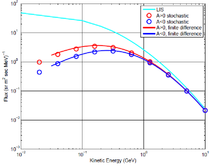
Figure 6: An example of the exhaustive benchmarking studies presented in earlier SDE-model papers. Although, in retrospect, these benchmarking studies seem superfluous (the mathematical equivalence is already established), they were needed in order to illustrate the validity of SDE approach to the heliospheric community. This example is taken from Pei et al. (2010).

The next step in modulation models was the implementation of a wavy HCS. This is, however, by no means an easy task to accomplish in 3D. The first model to achieve this was given by Miyake and Yanagita (2005); this work was summarized in a conference proceeding but never published in detail. A more detailed methodology (but only in 2D) was given by Alanko-Huotari et al. (2007), and for 3D models by Pei et al. (2012) and Strauss et al. (2012). The inclusion of a wavy HCS also gave the opportunity to effectively illustrate the drift process, and an example of such an illustration is shown in Fig. 7. Here the exit positions (that is, the position, in terms of polar and azimuthal angles, at which a pseudo-particle exits the heliosphere, i.e. reaches the edge of the computational domain) at a spherical heliopause for GCR proton pseudo-particles are shown. This representation needs some careful interpretation: The pseudo-particles are released at Earth and exits the heliosphere at the shown positions. In the time-forward scenario, it can thus be concluded that GCR, that enter the heliosphere at these positions, will end up at Earth. It does, however, not mean that GCRs only enter the heliosphere at these positions (the GCR flux is assumed isotropic and uniform outside the heliosphere). The simulations presented in Fig. 7 are performed for the $A>0$ (blue points) and $A<0$ (red points) drift cycles and varying values of the HCS tilt angle. In the $A>0$ drift cycle, GCR protons generally drift from the polar regions to reach Earth, whereas, in the $A<0$ cycle, they mainly drift along the HCS (for details see also Strauss et al., 2012). See also the modelling of Raath et al. (2016, 2015). The effectiveness of SDE-type models in modeling and reproducing drift effects, have recently led to SDE models being increasingly applied to model charge sign dependent modulation effects (e.g., Della Torre et al., 2012; Bobik et al., 2012; Maccione, 2013), that is, simultaneously modeling and reproducing particle and anti-particle ratios in order to gauge the effectiveness of the drifts in different polarity cycles.

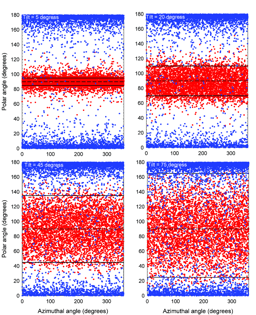
Figure 7: Illustrating drift effects in the heliosphere by plotting the exit position of protons in the so-called $A>0$ (blue) and $A<0$ (red) drift cycles for various tilt angles. The solid and dashed lines show the latitudinal extend of the wavy HCS, with the different tilt angles indicated on each panel. The figure is taken from Strauss et al. (2012). With permission of Springer.

From the onset, Zhang (1999) illustrated that, in the SDE formulation, it is possible to calculated the propagation (resident) time and energy losses suffered by GCRs directly. Strauss et al. (2011b) showed that these quantities, calculated numerically via a SDE model, compare well with earlier analytical models. Florinski and Pogorelov (2009), for example, calculated the propagation time for particles in different regions of the heliosphere and illustrated that they spend a long time in the heliosheath (the region between the termination shock and the heliopause); a region where CRs suffer little or no energy losses. Similarly, Bobik et al. (2011) included and illustrated the effect of additional deterministic energy loss processes. Although such calculations make the modulation process clearer and more understandable, it is not yet conclusively established how these quantities are related to CR intensities or observations (see e.g. Strauss et al., 2013, for an attempt at this). It must always be kept in mind that pseudo-particles are not real particles! More recent work by, e.g., Vogt et al. (2015), suggests more complicated weighting procedures for the propagation time in order for this quantity to be more representative of reality.

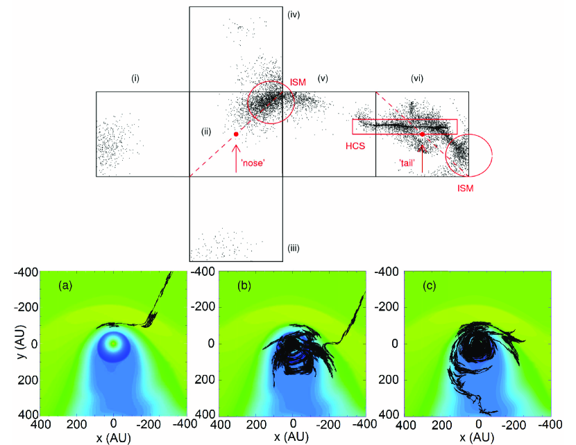
Figure 8: A solution of a hybrid CR modulation model, taken from Strauss et al. (2013). The bottom panels show the trajectory of 3 pseudo-particles in an MHD simulated heliospheric environment (the contour plots show the plasma density). The top panel shows the exit positions of pseudo-particles, initially released from Earth, at the boundaries of the model. For this scenario, the model boundary is a cube, which is “unfolded” in the top panel. The large red circles indicate the position of pseudo-particles that have entered the heliosphere by propagating along the assumed interstellar magnetic field (labelled ISM), while the red square shows particles which drifted along the heliospheric current sheet (labelled HCS). The “nose” and “tail” of the heliosphere are indicated on panels (ii) and (vi) respectively.

Due to the stability of the SDE numerical scheme, coupled with the low memory requirements when solving SDEs in higher dimensions, it has also become possible to create hybrid CR modulation models. These are models that use the input from magneto-hydrodynamic (MHD) models of the heliosphere geometry and plasma flow fields, and solve the TPE using essentially a test (pseudo-) particle approach (i.e. coupling the TPE to an MHD simulated background plasma). Such models can be considered more realistic in the sense that they capture the complex and asymmetrical structure of the heliosphere. The first of these models was presented by Ball et al. (2005), where after the approach was followed by Florinski and Pogorelov (2009), Strauss et al. (2013), Luo et al. (2013), Guo and Florinski (2014b) and most recently by Guo and Florinski (2014a). These models were mostly applied to GCR transport in the large-scale heliosphere (with the focus on the heliosheath; see also Section 3.1), while Guo and Florinski (2014a) modeled the effect of co-rotating interaction regions (CIRs) on GCR intensities in the inner heliosphere. An example solution of such a hybrid modulation model is shown in Fig. 8.

Although the numerical approach to integrating SDEs is, per definition, time dependent (it can be considered an explicit numerical scheme), most of the above-mentioned work considered the steady-state solution, i.e. all pseudo-particles are integrated until they reach a boundary. Some work that has focused on time-dependent (meaning here that the transport coefficients are time-dependent and no stationary solution exists) solutions is, however, available (e.g. Yamada et al., 1999; Luo et al., 2011; Guo and Florinski, 2014a; Wawrzynczak et al., 2015a).

2.5.3 Pseudo-particle interpretation and an illustration of Liouville’s theorem

Because the SDE model solves for $f(\vec{x},t)$, a pseudo-particle represents a realization of $f(\vec{x},t)$, so that a pseudo-particle is defined as an ensemble of CR particles, where the ensemble is constructed such that it results in a gyro- and isotropic collection of particles. A more accurate term for a pseudo-particle is that of a phase space density element. However, the nomenclature of a pseudo-particle is ingrained into the field of SDE based modulation models, and as such, will be used throughout this paper. Many discussions have shown that it is sometimes mistakenly assumed that a pseudo-particle represents an actual CR particle, or the guiding centre of such a particle. This is of course not the case, as a single GCR particle would follow the Lorentz-Newton equations of motion. The way in which particle source and/or loss terms are treated in the SDE approach (see Sections 4 and 5) also shows that pseudo-particles are in fact not physical particles; ‘pseudo’ may be assumed to refer to the fact that they are simply mathematical realizations of particle distribution functions (see also the comments by Kopp et al., 2012).

The trajectory of a pseudo-particle also has an often overlooked and very important physical significance. Along the trajectory of a single pseudo-particle (where $\vec{x}^{\prime}$ labels the set of phase space coordinates along this trajectory)

$$\rho(\mathcal{\vec{x}^{\prime}})=1,$$ (43)

which is an extension of Eq. 39, and occurs because of the normalization condition of $\rho(\vec{x},t)$ as shown in Eq. 39. Because $f(\vec{x},t)\propto\rho(\vec{x},t)$, it follows that

$$f({\vec{x}^{\prime}})=\mathrm{constant},$$ (44)

so that

$$\frac{Df({\vec{x}^{\prime}})}{Dt}=0,$$ (45)

which is a Lagrangian derivative along $\vec{x}^{\prime}$. Eq. 45 is simply a re-statement of Liouville’s theorem: Along the trajectory of a pseudo-particle through phase space, the CR distribution function remains constant. The trajectory of a pseudo-particle therefore also shows a graphical illustration of Liouville’s theorem. For cases, described later on, where sources and/or sinks of particles are considered, the phase-space distribution along the path of a pseudo-particle is no longer constant, and hence, the connection with Liouville’s theorem cannot be made.

3 Choosing the Correct Time Step: Diffusive Shock Acceleration and the Transport of Cosmic Rays Beyond the Heliopause

“Ford!” he said, ”there’s an infinite number of monkeys outside who want to talk to us about this script for Hamlet they’ve worked out.”

h2g2

In this section, we again consider the 1D PDE

$$\frac{\partial f(x,t)}{\partial t}=\frac{\partial}{\partial x}\left(\kappa(x)\frac{\partial f(x,t)}{\partial x}\right)$$ (46)

where $\kappa$ is no longer constant, but assumed to be

$$\kappa(x)=0.5+0.25\tanh\left(10x\right).$$ (47)

$\kappa(x)$, and its derivative, are shown in panels (a) and (b) of Fig. 9. Note that $\kappa(x)$ changes by a factor of three over a length scale of ${L}=0.5$; the meaning of which will become clear during this section.

The corresponding SDE formulation is

$$dx=\frac{d\kappa(x)}{dx}dt+b(x)dW$$ (48)

where $b(x)=\sqrt{2\kappa(x)}$.

We focus on the effect of changing the numerical step size $\Delta t$ in the SDE solver. For the simulation used here, no initial condition is assumed, with $f(x=-1,t)=0$ and $f(x=1,t)=1$ and the results are compared to those of the FD code at time $T=1$.

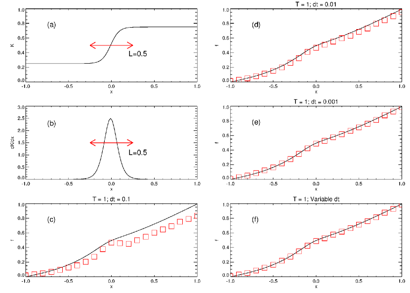
Figure 9: Comparing the SDE (open squares) and finite difference (solid line) methods for different choices of $\Delta t$. Panel (a) shows $\kappa(x)$, panel (b) its derivative and panels (c) - (e) the SDE results for $\Delta t=0.1$, $\Delta t=0.01$ and $\Delta t=0.001$ respectively. The SDE solutions in panel (f) adopt a variable time step.

Unlike finite differences, the SDE method does not have a prescribed restriction on the time step; i.e. no equivalent SDE CFL (Courant-Friedrichs-Lewy, see Courant et al., 1928) formulation is applicable. This has advantages, namely that the SDE method is therefore unconditionally stable. However, as we will show, the SDE solution does not converge to the correct solution if $\Delta t$ is chosen to be too large.

Panel (c) of Fig. 9 shows the results when $\Delta t=0.1$ is used in the SDE scheme (red squares) as compared to the FD scheme (solid line) which derives its value of $\Delta t$ from the appropriate CFL condition. This choice of $\Delta t$ is clearly too large and the comparison shows that the SDE results are clearly incorrect. In panel (d) a reasonable value of $\Delta t=0.01$ is adopted. However, the results of the SDE model, especially for $x>0$, is clearly still incorrect. Only for $\Delta t=0.001$ (panel e) do both numerical methods converge.

A question is however how to correctly choose the value of $\Delta t$? Our methodology to do this consistently starts with evaluating the first- and second-order moments of the SDE

$$\langle\Delta x\rangle = \frac{d\kappa(x)}{dx}\Delta t$$ (49)

$$\langle\Delta x^{2}\rangle = 2\kappa(x)\Delta t=b^{2}(x)\Delta t.$$ (50)

In the SDE approach, it can be assumed that the pseudo-particles, on average, move a distance $l^{2}=\max\left\{\langle\Delta x\rangle^{2},\langle\Delta x^{2}\rangle\right\}$ in a time step $\Delta t$. We can therefore use the numerical spatial step size to constrain the time step, i.e. by specifying a required average jump length $l$ we can determine what $\Delta t$ should be. For the diffusion equation we are currently considering, the transport parameters change over a spatial region of ${L}$. Assuming we want the pseudo-particles to sample this transition, we require that $l\ll{L}$. The time step is thus constrained by the expression

$$\Delta t(x)=\min\left\{\frac{l}{\left|\frac{d\kappa(x)}{dx}\right|},\frac{l^{2}}{b^{2}(x)}\right\}.$$ (51)

where $l$ is specified and must be therefore shorter than the shortest spatial structure present in the computational domain. Krülls and Achterberg (1994) state that a necessary requirement for an SDE model to be accurate is given $\langle\Delta x\rangle^{2}\ll\langle\Delta x^{2}\rangle$. Using our specific example, this imposes the following condition on the timestep, $\Delta t\ll 2\kappa/(d\kappa/dx)^{2}$, stating that the stochastic integration must be dominated by stochastic processes and not by deterministic drift terms. Depending on the integration scheme used, the deterministic terms may be traced, however, quite accurately (Kloeden and Platen, 1999).

For our present example, the smallest length scale of interest is that over which $\kappa$ changes and we choose $l=0.1{L}=0.05$. The results of the SDE scheme using this variable $\Delta t$ are shown in panel (f) of Fig. 9. It can be seen that for this choice of $\Delta t$ a good agreement exists between the SDE and FD schemes.

It is thus clear that, in order to correctly solve an SDE numerically, the modeled pseudo-particles must sample all features in the computational region. This can be done very efficiently, as illustrated in this section, by adopting a variable $\Delta t$, constrained by the first- and second-order moments of the SDE and prescribing the shortest length scale that must be sampled, $l$. Computationally, this is also much cheaper than using an artificially short time step over the entire spatial grid; $\Delta t$ is only reduced where e.g. $\kappa$ changes significantly but could be larger elsewhere.

3.1 Literature Review

In the previous section we have illustrated how crucial the choice of an appropriate time step is in a SDE model; the general rule of thump being that the pseudo-particles should sample the smallest region of interest in the computational domain. In the following section we discuss two scenarios for which this is especially important.

A further scenario was already alluded to in Section 2.5, namely that of drifts along the HCS. As shown by, e.g., Burger et al. (1985), CRs will experience the HCS, and start drifting along, when they are within 2 Larmor radii ($r_{L}$) from it. Therefore, based on the discussion in the previous section, we need to choose $\Delta t$ such that $l\ll 2r_{L}$ in order to capture the full effect of the HCS on CR modulation. Furthermore, because $r_{L}$ changes with both particle energy and spatial position (due to the changing HMF magnitude), is would be logical to implement a varying $\Delta t$ in such a numerical model.

3.1.1 Diffusive Shock Acceleration

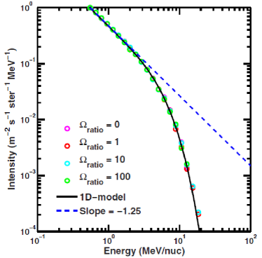
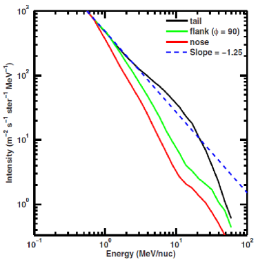
Figure 10: Simulating DSA with an SDE model, as applied to ACR acceleration at the TS (taken from Senanayake and Florinski, 2013). The left panel shows a comparison between the SDE results for spherically symmetric scenario (the symbols) and that of a 1D FD model (the solid line) as compared to the analytical result for an infinite planar shock (dashed line). The right panel shows the resulting ACR spectrum at the TS when a more realistic heliospheric geometry is incorporated, leading to preferred acceleration at some regions along the TS. © AAS. Reproduced with permission.

Without knowing its full implications, Fermi (1949) proposed the basis for shock acceleration: CR particles are scattered by forward and backward moving waves, making “head-on” (resulting in a kinetic energy gain) and “trailing” (resulting in a loss of kinetic energy) collisions. If the intensity of the forward and backward moving waves are roughly equal, the process can lead to diffusion of the original CR distribution function in energy space. The process is referred to as momentum diffusion, or Fermi II acceleration – referring to the fact that the energy gain per collision cycle is $\sim\left(v/c\right)^{2}$, where $v$ is particle speed and $c$ is the speed of light. In the presence of a shock wave (where the supersonic flow slows to subsonic speeds), and assuming the CRs have mobility across the shock, the process is much more efficient – CRs make more head-on collisions when moving upstream of the shock than trailing collisions when moving downstream – and the process is referred to Fermi I acceleration (the energy gain per collision cycle is $\sim v/c$), or more frequently, diffusive shock acceleration (DSA) . DSA is considered the dominant process responsible for particle acceleration at supernovae blast waves (thus creating the GCR component) and, more, locally at the heliospheric termination shock (TS, thus creating the anomalous cosmic ray (ACR) component), while travelling interplanetary shocks can also energize CRs. DSA can be modeled in the Parker formalism, by noting that the plasma flow divergence term, $\nabla\cdot\vec{u}$, governing energy changes, becomes large and negative at a shock, and if treated correctly, can be used to simulate DSA on the distribution function level. For details, see the comprehensive review by Drury (1983), or, more recently, by Fichtner (2001).

In order to numerically model DSA, Parker’s equation needs to be solved, accounting for the large value of $\nabla\cdot\vec{u}$ directly at the shock. Mainly for numerical reasons, but also motivated by physical arguments (see e.g. le Roux et al., 1996), the shock is taken to have a finite width (denoted by $L_{\mathrm{shock}}$). In the SDE formulation, the pseudo-particles should therefore sample this acceleration region $L_{\mathrm{shock}}$ continuously and not only interact with the shock sporadically. In the terminology of the previous section, the numerical step size should be such that $l\ll L_{\mathrm{shock}}$. A thorough discussion regarding this, and SDE model solutions including DSA, are given by Achterberg and Krülls (1992), Krülls and Achterberg (1994), Park and Petrosian (1996), Marcowith and Kirk (1999) and more recently by Achterberg and Schure (2011). The technique of using a variable $\Delta t$, as illustrated in the preceding section, is thus ideally suited for simulating DSA at quasi-discontinuous shocks via SDE models .

The acceleration of ACRs at the TS was recently modeled, utilizing a SDE approach, by Senanayake and Florinski (2013), with some of their results shown in Fig. 10. The acceleration of ACRs proved to be a contentious research topic after Voyager 1 did not observed the expected power law spectrum at the TS (e.g. Stone et al., 2005; Decker et al., 2005), but rather a modulated form. Although several explanations followed, including the inclusion of momentum diffusion into the transport model (e.g. Strauss et al., 2010), this modulated form is generally attributed to more efficient acceleration of ACRs at certain positions along the TS, also evident from the results shown in Fig. 10.

Recently, modeling DSA for anisotropic particle distributions, i.e. adopting the more general Skilling (1971) transport equation, has attracted some attention, with Zuo et al. (2011, 2013) and Kartavykh et al. (2016) applying a pitch-angle dependent SDE model.

3.1.2 Outer Heliosheath Modulation

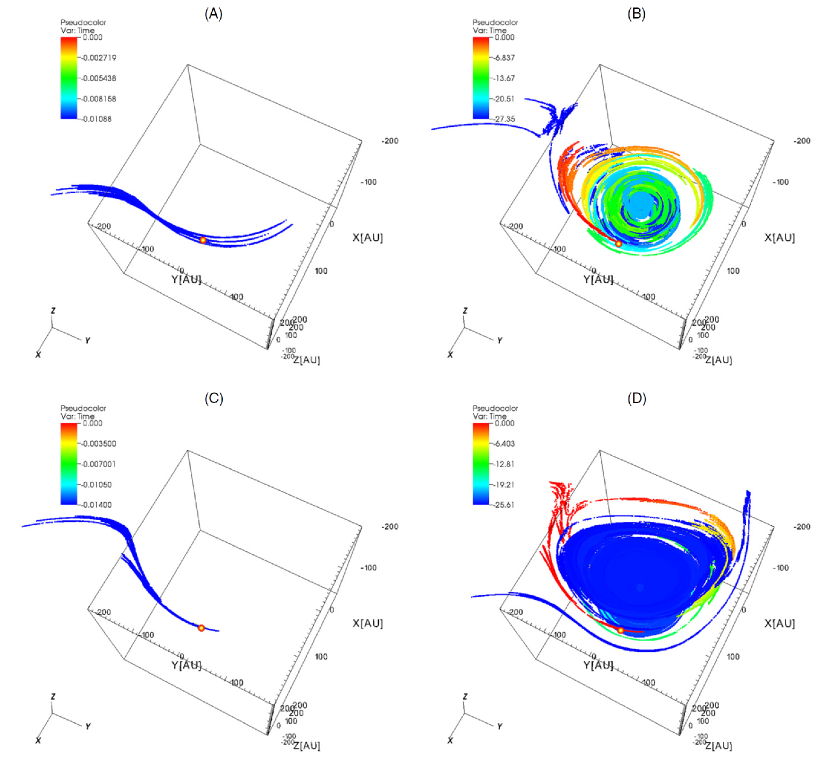
Figure 11: An example of pseudo-particle trajectories in a hybrid CR modulation model, taken from Guo and Florinski (2014b). Although the diffusion coefficients change by orders of magnitude across the HP, a variable $\Delta t$ forces the pseudo-particles to sample different regions of the computational regime with the same spatial precision. Here, the authors choose $l$ to be smaller than the grid size of the MHD model. This is essential to capture the full effect of CR modulation across the HP. © AAS. Reproduced with permission.

Anticipating the Voyager crossing of the HP, Scherer et al. (2011) questioned the use of a Dirichlet boundary condition for GCR modulation at the HP . Because GCRs diffuse through both the heliosphere and the local interstellar medium, it is quite conceivable that GCRs might “leak” into the heliosphere faster than they are replenished from the galaxy, leading to a positive gradient outside the HP. If this is true, the LIS for GCRs (i.e. the Dirichlet boundary condition) must be places at some distance beyond the HP (the region between the HP and the bow-shock if referred to as the outer heliosheath; the region of interstellar plasma still influenced by the presence of the heliosphere). A study by Scherer et al. (2011), using SDEs, and a follow-up study by Herbst et al. (2012) found that this might be the case, depending on the assumed parameters. Kóta and Jokipii (2014), using a semi-analytical model, however, suggested that GCR modulation beyond the HP is not possible.

The models mentioned in the previous paragraph are simplified, to such an extent that they may not be able to capture the complex nature of GCR transport beyond the HP. To mitigate this, Strauss et al. (2013) applied a hybrid GCR modulation model to the problem (see also the discussion in Section 2.5.2). From a modeling point-of-view, the transport of GCRs across the HP presents an intriguing problem: The diffusion coefficients across the HP change by up to a factor of $10^{5}$, due to the different turbulent processes believed to occur in these distinct regions (the HP can be considered a tangential discontinuity so that the two plasmas – the heliospheric plasma on the one side and the interstellar medium on the other – cannot mix and interact). This large, fairly abrupt change in $\mathbf{K}$ leads to a large $\nabla\cdot\mathbf{K}$ drift type term that, if handled incorrectly, can lead to incorrect results. For this reason, Strauss et al. (2013) employed a variable $\Delta t$, in a similar fashion to Eq. 51, mimicking a SDE-type CFL condition. The pseudo-particles can, therefore, not have unreasonable high propagation speeds and are able to sample the HP region sufficiently. Results from this paper corroborated that of Scherer et al. (2011): Modulation beyond the HP is possible, but the level of modulation is heavily parameter-dependent. Two more hybrid GCR modulation models that addressed this possibility followed; firstly by Guo and Florinski (2014b) (with some of their results highlighted in Fig. 11) and recently by Zhang et al. (2015) and Luo et al. (2015). Although the latter confirmed the results of Strauss et al. (2013), the former rejected these. The question of whether modulation of GCRs beyond the HP occurs, and therefore also whether a Dirichlet boundary condition at the HP is appropriate, remains unanswered.

Directly after crossing the HP, Voyager 1 measured anisotropic CR distributions in the interstellar medium (Krimigis et al., 2013). This necessitates the use of a pitch-angle dependent CR transport equation (e.g. Skilling, 1971), rather than the Parker equation, valid only for isotropic CR distributions. Due to the strong gradients emphasized earlier in this section, SDE models were again applied to the problem by Florinski et al. (2013) and Strauss and Fichtner (2014). Explaining these anisotropies remains an ongoing topic of study.

4 Handling Source/Sink Terms: Galactic Cosmic Ray Propagation

We demand rigidly defined areas of doubt and uncertainty!

h2g2

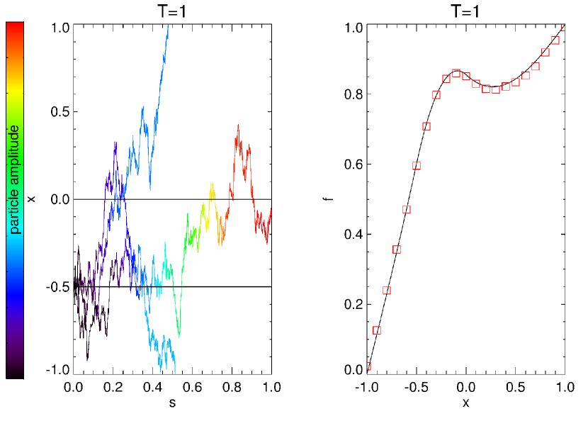
Figure 12: The left panel shows traces of pseudo-particles starting at $x=-0.5$, colored according to their amplitude as given by Eq. 55: Initially $a=0$ (as indicated by black), but $a$ increases when the pseudo-particles interact with the source region. The right panel again compares the results of the SDE and FD models, using $10000$ particles at each $x$ point in the SDE approach.

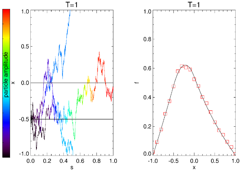
Figure 13: Similar to Fig. 12, but using the boundary conditions $f(x=-1,t)=f(x=1,t)=0$.

We consider again the 1D diffusion equation,

$$\frac{\partial f(x,t)}{\partial t}=\kappa\frac{\partial^{2}f}{\partial x^{2}}+Q(x)$$ (52)

with $\kappa=0.5$ constant, but with the addition of a source term $Q(x)$, given by

$$Q(x)=\left\{\begin{array}[]{l}2:x\in[-0.5,0]\\ 0:\text{otherwise}.\end{array}\right.$$ (53)

The equivalent SDE formulation is once again

$$dx=bdW,$$ (54)

but, with the addition of sources, a particle amplitude $a$ needs to be calculated along the integration trajectory for each pseudo-particle. This quantity is initially zero for each pseudo-particle $a_{i}^{s=0}=0$ (where $i$ refers to a single particle). The value of $a$ then changes during integration as

$$a_{i}(s+ds)=a_{i}(s)+Q(x)ds.$$ (55)

The value of $a$ can be positive (as in our example where a source is considered), but can also be negative (if sinks are considered, i.e $Q<0$).

To calculate $f$, Eq. 12 now needs to be generalized to account for the varying particle amplitude

$$f(x,T)=\underbrace{\int_{0}^{T}\int_{x}G(x^{\prime},t)f_{b}(x^{\prime},t)dxdt}_{\text{contribution from boundary conditions}}+\underbrace{\mathcal{A}(x,T)}_{\text{source contribution}},$$ (56)

where

$$\mathcal{A}(x,T)=\frac{1}{N}\sum_{i=1}^{N}a_{i}(s=T)$$ (57)

in its discretized form and where $N$ is the total number of pseudo-particles solved at a given $x$.

The particle amplitude can be considered as a “correction term” when sources/sinks are considered. This can be understood when re-writing Eq. 52 as

$$\frac{\partial f(x,t)}{\partial t}=\kappa\frac{\partial^{2}f}{\partial x^{2}}+\frac{da}{dt}$$ (58)

with the auxiliary equation

$$\frac{da}{dt}=Q(x)\Rightarrow\Delta a=Q(x)\Delta t$$ (59)

which must be solved simultaneously. The “standard” SDE methodology is followed to solve the diffusion part, while $a$ (the particle amplitude) is updated continuously along the pseudo-particle’s trajectory by solving Eq. 59, via Eq. 55, and adding the averaged correction term, $\mathcal{A}$, in Eq. 56.

The SDE solutions are presented in Fig. 12 using the boundary conditions $f(x=-1,t)=0$ and $f(x=1,t)=1$. The right panel of the figure shows a comparison between the SDE solutions (red squares) and a FD scheme (solid line), showing good agreement. The left panel shows the trajectory of 3 pseudo-particles originating from $x=-0.5$, where the curves are colored according to their particle amplitude (black corresponds to a zero value and red to a high positive value). It is clear that $a_{i}$ changes when the source region is encountered.

Fig. 13 is similar to Fig. 12, but this time using the boundary conditions $f(x=-1,t)=f(x=1,t)=0$. For this case, the only contribution to $f$ is from the $\mathcal{A}$ term in Eq. 56.

4.1 Galactic cosmic ray propagation studies

The transport of cosmic rays (CRs) in our galaxy is a topic of considerable interest, both from a fundamental point of view and due to its connection to the questions of CR origin and acceleration (Schlickeiser, 2002; Strong et al., 2007). It is furthermore believed that the CR component of the interstellar medium plays an important role in its overall dynamics, for example in the generation of the galactic magnetic field through dynamo processes (e.g. Hanasz et al., 2009), or galactic wind production (e.g. Fichtner et al., 1991; Breitschwerdt et al., 1991; Everett et al., 2010). A very recent overview on CR transport and its historic development can, for example, be found in Schlickeiser (2015).

In the past, most of the detailed numerical studies of galactic CR propagation relied on grid-based schemes to solve the diffusion-convection transport equation. The most widely used tool in the community, GALPROP (Strong and Moskalenko, 1998), for example, is based on a finite-difference scheme. The SDE approach offers a distinct alternative to such grid-based schemes. In particular, with the time-backward method, the distribution function can be calculated to high precision for a few phase-space points of interest, without any restriction from numerical stability and the need for a highly resolved computational grid for the entire galaxy. However, to enable CR modeling for the galactic transport problem, a proper treatment of CR sources, as introduced in this section, is essential.

4.1.1 The Galactic transport problem

Similar to the transport equation in CR modulation (Eq. 32), the propagation of CRs in the galaxy is described by a diffusion-convection equation for the differential galactic CR intensity $j(\vec{r},p,t)=p^{2}f(\vec{r},p,t)$ (e.g. Strong et al., 2007):

$$\frac{\partial j}{\partial t}=\nabla\cdot\left(\mathbf{K}\nabla\,j-\vec{u}j\right)-\frac{\partial}{\partial p}\left[\dot{p}j-\frac{p}{3}(\nabla\cdot\vec{u})j\right]+Q$$ (60)

where we have neglected already any momentum diffusion and $\vec{u}$ denotes again the effect of combined background advection effects, e.g. of a galactic wind. Momentum loss processes enter the coefficient $\dot{p}$; for protons in the GeV energy range, for example, the dominant loss processes are ionization and pion production (e.g. Mannheim and Schlickeiser, 1994). Further linear terms can appear in the equation to describe catastrophic losses or sources of particles, through spallation and/or annihilation reactions (e.g. Büsching et al., 2005; Blasi and Amato, 2012). Although the diffusion of CR particles is in general given by a diffusion tensor $\mathbf{K}$, the majority of studies up to now have assumed only a single scalar diffusion coefficient. $Q$ represents the combination of all CR sources, like for example supernova remnants, pulsars or even astrospheres of other stars (Scherer et al., 2008, 2015). A transport equation like Eq. 60 can be solved for any CR species of interest, and they are coupled by a complicated nuclear reaction network (Strong et al., 2007).

4.1.2 Selected results

Instead of elaborating further about the many details that enter the CR transport equation, we restrict ourselves here to a concise discussion of some of the recent studies that made use of the SDE solution method and those related to them.

One of the first studies to use the complete SDE equivalence for the solution of the galactic transport equation was Farahat et al. (2008). They already employed a sophisticated nuclear reaction network and benchmarked their model by comparing their resulting primary to secondary ratios with previous GALPROP calculations by Strong and Moskalenko (1998) and observations. They particularly emphasized the usefulness of the backward time integration to determine the distribution at specific positions in the galaxy and also the easy treatment of extended sources with this method.

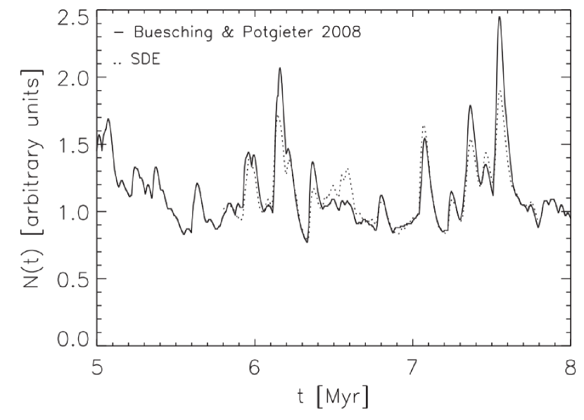
Figure 14: From Kopp et al. (2014): Temporal variation of the cosmic ray flux for 1 GeV protons for an inter-arm region. The solid line gives the Büsching and Potgieter (2008) result, while the dashed line is obtained by the novel SDE code with the same set of point sources. Reprinted with permission from Elsevier.

The influence of CR source distributions on the CR flux variation throughout the galaxy has gained increased attention in recent years. Büsching and Potgieter (2008) already considered a source distribution consisting of more than a hundred thousand discrete supernova remnants (SNRs) with locations following the galactic spiral pattern (e.g. Vallée, 1995, 2014). In their study, they did not employ an SDE method but rather numerics based on a Fourier-Bessel series and a Crank-Nicholson scheme. Their results served as a benchmark for the study by Kopp et al. (2014), in which the SDE method was used to solve a similar problem (see Fig. 14). Furthermore, they considered the influence of a spatial variation of the diffusion coefficient with the spiral arm pattern. Both studies show a significant variation of the CR flux along the solar orbit around the galactic center (i.e. between arm and inter-arm regions) as well as shorter temporal variations due to the discreetness of the sources in space and time. Different spiral source distributions have also recently been studied by Werner et al. (2015) and Kissmann et al. (2015) using novel grid based elliptic solvers (Kissmann, 2014).

Another study on the influence of discrete sources using the SDE method has recently been published by Miyake et al. (2015). They show how the SDE method can yield path lengths and age distributions for the arrival of CRs at Earth, thus emphasizing the strong influence of discrete sources on the observed flux and primary/secondary ratios. These aspects have been discussed already earlier by, e.g. Blasi and Amato (2012) and Mertsch (2011).

The backward SDE methods was employed in Effenberger et al. (2012b) to study the influence of a full diffusion tensor on the GCR propagation in a continuous spiral source model. The background galactic magnetic field was chosen to be aligned with the spiral arm pattern so that the diffusion could be set to a smaller value perpendicular to the arms.

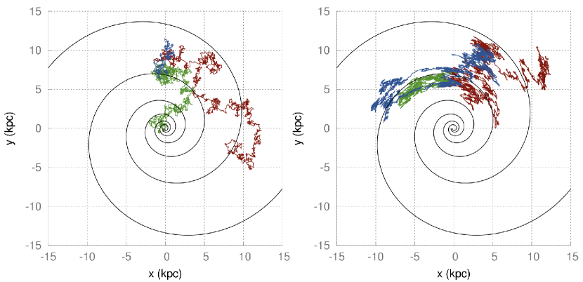
Figure 15: From Effenberger et al. (2012b): Exemplary pseudo-particle trajectories in the galactic magnetic field, projected onto the galactic plane. The left panel is for isotropic diffusion while the right panel shows the effect of anisotropic diffusion with $\kappa_{\perp}/\kappa_{\parallel}=0.1$. Reproduced with permission from Astronomy & Astrophysics, © ESO.

Figure 15 shows how the trajectories of pseudo particles allow to visualize how the phase-space is traced differently when anisotropic diffusion is considered, i.e. when the diffusion along the mean magnetic field, $\kappa_{||}$, is more effective than diffusion perpendicular to it, $\kappa_{\perp}$. Anisotropic diffusion was found to be also of importance for the details and efficiency of galactic magnetic dynamo action (Hanasz et al., 2009; Pakmor et al., 2016).

5 Importance Sampling: Solar Energetic Particle Transport and Diffusive Shock Acceleration

One of the things Ford Prefect had always found hardest to understand about humans was their habit of continually stating and repeating the very very obvious.

h2g2

Consider the diffusion equation with a convective part added

$$\frac{\partial f(x,t)}{\partial t}=V\frac{\partial f}{\partial x}+\kappa\frac{\partial^{2}f}{\partial x^{2}}$$ (61)

where we choose $V=-2$ and $\kappa=0.5$ as constants.

The equivalent SDE formulation is

$$dx=Vdt+bdW$$ (62)

Using the boundary conditions, $f(x=-1,t)=0$ and $f(x=1,t)=1$, Fig. 16 shows the solution at $T=1$. The left panel shows pseudo-particle traces for $50$ particles, starting from $x=-0.5$, along with the average position of the particles $y=\langle\Delta x\rangle$ (dashed red line; the first-order moment) and the $1\sigma$ deviation from this value, $y^{\prime}=\langle\Delta x\rangle\pm\sqrt{\langle\Delta x^{2}\rangle}$ (solid red line; essentially the second-order moment). The right panel shows the solution of the finite difference model (solid line) and the SDE model (symbols). Three cases for the SDE model are shown (denoted by the different symbols). These correspond to the same simulation ($100$ pseudo-particles at each position) but using different sequences of Wiener processes, i.e. each time the integration process is initiating with a different seed.

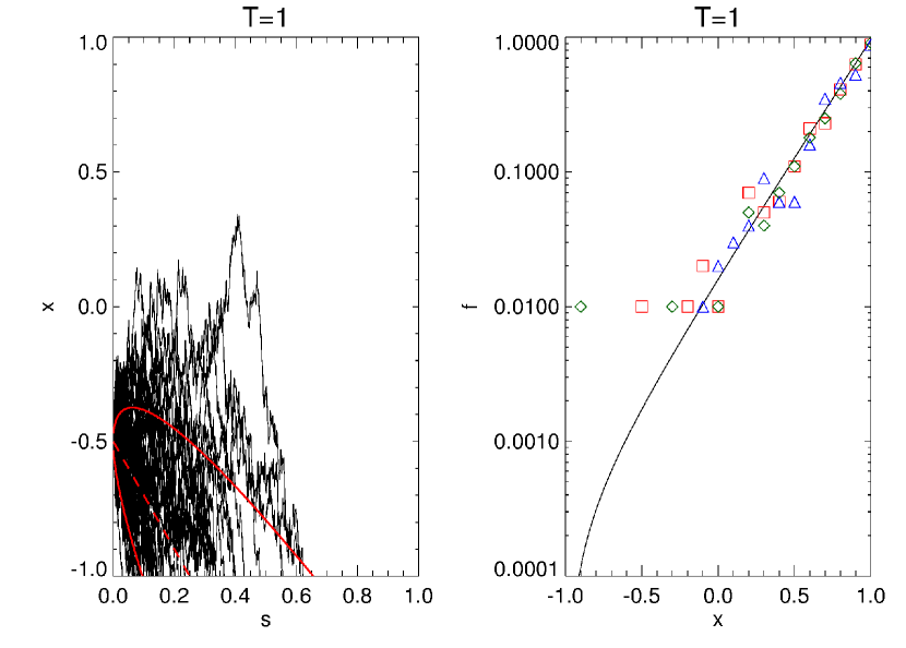
Figure 16: The left panel shows $50$ pseudo-particle traces starting from $x=-0.5$, while the right panel compared the finite difference (solid line) and SDE solutions (symbols) using three different sequences of Wiener processes.

For the set-up discussed above, the SDE model runs into problems with the statistics of the resulting pseudo-particles. With the large negative value of $V$, the pseudo-particles are convected towards smaller $x$ and hence only a very limited number interact with the non-zero boundary at $x=1$. With so few particles reaching it, the statistics of the solution decreases, i.e. the SDE solution becomes more noisy. This is clear from the right panel of the figure, which illustrates that, especially for $x<0$, the SDE solution oscillates around the actual solution. As $x\rightarrow-1$, this effect of course increases with the SDE solution showing a very coarse discrete nature, i.e. if only $1$ in $100$ particles interact with the boundary, the value of $f$ becomes $f=0.01$. For two particles, $f=0.02$, etc.

There are two ways in which to overcome this difficulty. This first is to increase the number of pseudo-particles used. This brute-force method is however computationally very expensive, and does not imply much better statistics. A second, perhaps more elegant method would be to implement an “importance sampling” technique. We discuss here a hands-on method to implement importance sampling for our present model in order to enhances the statistics of the SDE solution near $x=-1$. The basic idea is to add (in a self-consistent manner) an additional and artificial convective term into the SDE equation, thereby forcing the pseudo-particles to sample a spatial region we are interested in. For this case, we want them to be convected more towards $x=1$.

We start by converting the original $f(x,t)$ to a modified function $g(x,t)$,

$$A(x)g(x,t)\equiv f(x,t)$$ (63)

where $A(x)$ is a function chosen later on. As will be shown below, the dependence of $A(x)$ on $x$ will lead to the desired additional convection speed in the $x$-coordinate. The relevant PDE is now

$$\frac{\partial g(x,t)}{\partial t}=\left(V+2\frac{\kappa}{A}\frac{dA}{dx}\right)\frac{\partial g}{\partial x}+\kappa\frac{\partial^{2}g}{\partial x^{2}}+\left(\frac{V}{A}\frac{dA}{dx}+\frac{\kappa}{A}\frac{d^{2}A}{dx^{2}}\right)g$$ (64)

which includes an additional convective term, so that the total convective term becomes

$$V^{\prime}=\underbrace{V}_{\text{original convection}}+\underbrace{2\frac{\kappa}{A}\frac{dA}{dx}}_{\text{artificial convection}}$$ (65)

where the additional convective speed can be chosen arbitrarily in order to increase the statistics of the SDE solver. Note that this equation also has a linear gain/loss term with a coefficient,

$$\mathcal{L}=\frac{V}{A}\frac{dA}{dx}+\frac{\kappa}{A}\frac{d^{2}A}{dx^{2}}$$ (66)

which needs to be taken into account and is discussed below.

The equivalent SDE formulation is then

$$dx=V^{\prime}dt+bdW,$$ (67)

with the addition that, because linear terms are present in the PDE, the particle weight for each pseudo-particle also needs to be evaluated at each time step,

$$\alpha_{i}(s+ds)=\alpha_{i}(s)\exp\left\{\mathcal{L}(x_{i}(s))ds\right\}$$ (68)

where, initially $\alpha_{i}(s=0)=1$ and the index $i$ refers to a single pseudo-particle.

Similarly to the particle amplitude discussed in the previous section, the particle weight is a correction introduced when linear terms are present in the PDE. Casting Eq. 64 into the form

$$\frac{\partial g(x,t)}{\partial t}=V^{\prime}\frac{\partial g}{\partial x}+\kappa\frac{\partial^{2}g}{\partial x^{2}}+\frac{d\alpha}{dt}$$ (69)

with, once again, an axillary term

$$\frac{d\alpha}{dt}=\mathcal{L}\alpha\Rightarrow\Delta\alpha=\exp\left\{\mathcal{L}\Delta t\right\}.$$ (70)

The standard SDE methodology is used to solve the diffusion equation, while the particle weight accounts for the axillary equation, Eq. 70, by solving it, via Eq. 68, along the trajectory of each pseudo-particle.

Say, for our example, we require that

$$V^{\prime}=V+2\frac{\kappa}{A}\frac{dA}{dx}=1,$$ (71)

i.e that the artificially introduced convection speed counteracts the original convection speed. The required value of $A(x)$ is readily evaluated (once again we choose $V=-2$ for the actual convection speed),

$$\frac{1}{A}\frac{dA}{dx}=\frac{d\ln A(x)}{dx}=3\Rightarrow A(x)=Ce^{3x}.$$ (72)

Note that the value of the integration constant, $C$, cancels in all calculations. These values will be used in the following simulations to illustrate the effectiveness of the importance sampling technique in enhancing the statistics of the normal SDE solver.

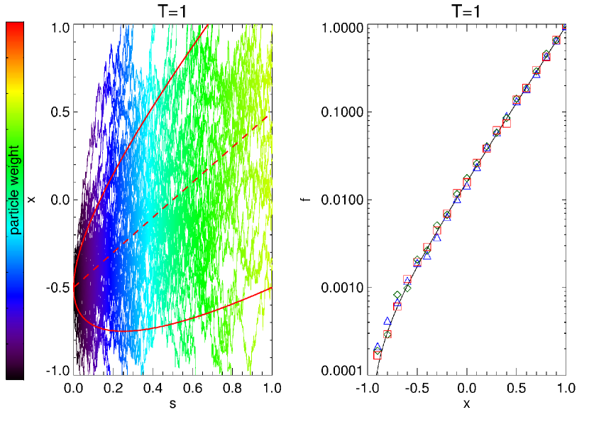
Figure 17: Similar to Fig. 16, but now with the inclusion of importance sampling.

Similar to the particle amplitude, the value of an individual pseudo-particle’s weight also enter the calculation of $f$, but this time, changing $G(x,T)$ directly. When a particle reaches a temporal or spatial integration boundary, it is not counted (in the discretized version) as a single particle, but as a fraction $\alpha_{i}(s=T)$ of a particle (depending on the sign of $\mathcal{L}$ this fraction may be either smaller or larger than unity). In Eq. 18 the binning procedure was explained, for the case of no linear terms, as counting the number of pseudo-particles in each bin $(N_{j})$ and normalizing by the total number of particles $(N)$, i.e.

$$G(x,T)dx\approx\frac{N_{j}}{N}=\frac{1}{N}\sum_{i=1}^{N_{j}}1$$ (73)

when $\alpha\neq 1$ (i.e. when linear terms are introduced) this now becomes the addition of non-integers e.g.

$$G(x,T)dx\approx\frac{1}{N}\sum_{i=1}^{N_{j}}\alpha^{i}(s=T).$$ (74)

The convolution with the boundary condition remains unchanged, although the normalization condition is no longer true

$$\int_{x}\int_{t}G(x,t)dtxt\neq 1.$$ (75)

The results of this modified PDE are shown in Fig. 17. The left panel shows again the pseudo-particle traces (technically now used to calculate $g(x,t)$), colored according to the particle weight, while the right compares the calculated $f(x,t)$ to the finite difference model. Now, all regions of the computational region have adequate sampling and more accurate solutions are obtained. The number of solved pseudo-particle trajectories are the same as in Fig. 16, but the statistics of the solution is much better, especially near the $x=-1$ boundary.

5.1 Literature Review

The importance sampling technique appears to be applicable in any modeling scenario where problems related to pseudo-particle statistics are present, i.e. pseudo-particles, due to the processes they represent, are unable to reach model boundaries, cannot contribute to the intensity, and hence, become redundant in some sense. This technique has not been implemented extensively in astrophysical SDE applications, although a limited number, discussed below, of such implementations do exist.

5.1.1 Solar Energetic Particles

Solar energetic particles (SEPs) are energetic particles accelerated near the Sun during transient solar events. As reviewed by Reames (2013), SEPs events can be divided into two classes: So-called impulsive events, where SEP acceleration is believed to occur at solar flares and gradual events, where the acceleration is though to occur at the shock associated with a propagating coronal mass ejection. Primarily due to very efficient focussing near the Sun (the diverging HMF tends to focus the SEPs into a narrow beam), any SEP distribution is usually highly anisotropic (in terms of pitch-angle), so that the Parker (1965) TPE cannot be used to model their propagation. A more general, focused transport approach is needed (e.g. Roelof, 1969; Skilling, 1971; Ruffolo, 1995; Litvinenko, 2012; Litvinenko and Noble, 2013; Effenberger and Litvinenko, 2014; Litvinenko et al., 2015; Strauss and Fichtner, 2015). We also mention that some models of pick-up ion transport in the heliosphere, like for example in Chalov et al. (1995) and Fichtner et al. (1996), employ SDE methods which are related to SEP transport models in many aspects. These applications are not discussed further in this review.

The transport of SEPs has been modelled extensively, using the time forward SDE formalism, by e.g. Dröge et al. (2010), Dresing et al. (2012), Dröge et al. (2014) and Laitinen et al. (2015). When simulating SEP events in the time-backward SDE framework, a problem related to pseudo-particle statistics is, however, present: Starting from, e.g., Earth, the pseudo-particles are traced, as always, back towards their source, which, for SEPs, is a small spatial region close to the Sun. The problem is that only an extremely small fraction of the pseudo-particles will reach this small source region; this is clear by simply comparing the volume of the source region (usually placed at $r=0.005$ AU) to that of the simulation volume (with an outer boundary placed at a minimum distance of $r=3$ AU), to give the expected probability of SEPs reaching the source region as $\sim 5\times 10^{-7}$ %. To overcome this difficulty, Qin et al. (2005) and Zhang et al. (2009) implemented an importance sampling technique, along the lines discussed in this work, very successfully. In essence, an artificial convective velocity is added to advect the pseudo-particles towards the inner boundary. If such an additional convective speed is included in a self-consistent manner, as illustrated in the previous paragraph, the results are both valid, and have much increased statistics. See also the more recent modelling of e.g. Qin and Wang (2015).

We further want to note here that also in the context of solar flare physics SDEs have been employed successfully. The Fokker-Planck equation used to describe the particle acceleration in a flare is very similar to the transport equations discussed previously. It describes the energy gains through a second order process in momentum, which is due to interactions with the turbulence background created by the reconnection events during a flare (e.g. Petrosian, 2012). MacKinnon and Craig (1991) noted already early that the evolution of the electron distribution in space and pitch-angle due to binary collisions can be described by an equivalent set of ordinary stochastic differential equations. Fletcher (1995), Fletcher (1997) and Jeffrey et al. (2014) applied the SDE method to the impulsive loop-top emission of solar flares and their trapping due to magnetic fields (Fletcher, 1997) and Park and Petrosian (1996) compared different solution methods for the flare acceleration problem. More generally, the stochastic acceleration of solar flare protons and electrons has been discussed by e.g. Barbosa (1979); Schlickeiser and Steinacker (1989); Miller and Roberts (1995) and Petrosian and Liu (2004).

5.1.2 Shock Acceleration

A problem with pseudo-particle statistics may also be present when simulating DSA in a time-backward fashion: The pseudo-particles are initially released, e.g., at the acceleration region (shock) with an energy of $\sim 100$ MeV. These particles, in the time-backward scenario, constantly loose energy while being in the acceleration region, until some of them might reach the injection energy of the source population - this injection energy is usually much lower than the energies of interest, e.g., $\sim 100$ keV. For an ensemble of pseudo-particles, at any higher energy, to have any contribution to the total intensity, they therefore have to sample the acceleration region long enough to reach the injection energy. Because spatial diffusion is also present, the likelihood of this happening is extremely low, and an importance sampling technique can be applied to remedy the lack of pseudo-particle statistics, and interestingly, this can be accomplished by two very different approaches.

The first approach would be to increase the amount of time a pseudo-particle spends in the acceleration region. For example, to include an artificial spatial advective speed to force the pseudo-particles back towards the shock region. A second, and perhaps more elegant approach, is to include an artificial convection speed in energy space, so that the pseudo-particles reach the injection energies faster. The latter approach was followed by Zhang et al. (private communication, 2015), who concluded that such a modification in an SDE model leads to an increase in pseudo-particle statistics, while reproducing the standard SDE results.

6 Summary

Forty-two

h2g2

The transport equations describing the propagation of non-thermal particles through turbulent plasmas have, in recent years, become increasingly complex and must therefore be integrated numerically. An increasingly popular numerical method is the use of SDEs. In this review paper we have tried to give a practical introduction to SDEs and how these equations are solved numerically for a variety of Fokker-Planck type transport equations arising in different fields of space- and astrophysics. We have focussed on possible numerical pit-falls that may arise, e.g., choosing an appropriate time-step, and, demonstrated how to overcome these issues by solving simpler 1D “toy models”. These models also included discussions regarding the handling of sources/sinks and linear gain/loss terms in the SDE formulation by keeping track of the so-called particle amplitude and weight, and introduced a hands-on technique of incorporating importance sampling in an SDE model. After each technical section, we gave a brief overview of the current literature that have applied these techniques, and presented selected results.

It is noteworthy to point to the possibility of further extensions of the SDE scheme to non-diffusive, in particular sub- and superdiffusive processes (e.g. Magdziarz and Weron, 2007; Effenberger, 2014; Stern et al., 2014). The basic idea is to generalize the Wiener process in the SDE formulation to a wider class of stochastic processes, for example so called Lévy or $\alpha$-stable processes, which describe the deviations from Gaussian-like diffusion behavior. This in turn can lead to more “heavy-tailed” distributions and power-laws instead of exponentials in particle configuration space or energy. We recommend the reviews by Perrone et al. (2013) and Zimbardo et al. (2015) to the interested reader, who wants to learn more about the physics background and applications of these concepts.

Although, from our experience in writing this review, the number of studies using the SDE method in space physics and astrophysics is still limited, the trend in the last years is certainly encouraging. The advantages of SDE formulations and numerics for a large class of particle kinetics problems due to the opportunities for parallel computing are significant. With this review, it is our hope that we could provide a contribution in enabling future studies using this powerful and yet simple method.

Exactly!” said Deep Thought. ”So once you do know what the question actually is, you’ll know what the answer means.