Lasso ANOVA Decompositions for Matrix and Tensor Data

Abstract

Consider the problem of estimating the entries of an unknown mean matrix or tensor given a single noisy realization. In the matrix case, this problem can be addressed by decomposing the mean matrix into a component that is additive in the rows and columns, i.e. the additive ANOVA decomposition of the mean matrix, plus a matrix of elementwise effects, and assuming that the elementwise effects may be sparse. Accordingly, the mean matrix can be estimated by solving a penalized regression problem, applying a lasso penalty to the elementwise effects. Although solving this penalized regression problem is straightforward, specifying appropriate values of the penalty parameters is not. Leveraging the posterior mode interpretation of the penalized regression problem, moment-based empirical Bayes estimators of the penalty parameters can be defined. Estimation of the mean matrix using these these moment-based empirical Bayes estimators can be called LANOVA penalization, and the corresponding estimate of the mean matrix can be called the LANOVA estimate. The empirical Bayes estimators are shown to be consistent. Additionally, LANOVA penalization is extended to accommodate sparsity of row and column effects and to estimate an unknown mean tensor. The behavior of the LANOVA estimate is examined under misspecification of the distribution of the elementwise effects, and LANOVA penalization is applied to several datasets, including a matrix of microarray data, a three-way tensor of fMRI data and a three-way tensor of wheat infection data.

1 Introduction

Researchers are often interested in estimating the entries of an unknown $n\times p$ mean matrix $\boldsymbol{M}$ given a single noisy realization, $\boldsymbol{Y}=\boldsymbol{M}+\boldsymbol{Z}$, where the entries of $\boldsymbol{Z}$ are assumed to be independent, identically distributed mean zero normal random variables with unknown variance $\sigma^{2}_{z}$. Consider a noisy matrix $\boldsymbol{Y}$ of gene expression measurements for different genes and tumors. Researchers may be interested in which tumors have unique gene expression profiles, and which genes are differentially expressed across different tumors.

This is challenging because no replicates are observed. Each unknown $m_{ij}$ corresponds to a single observation $y_{ij}$, and so the maximum likelihood estimate $\boldsymbol{Y}$ has high variability. Accordingly, simplifying assumptions that reduce the dimensionality of $\boldsymbol{M}$ are often made. Many such assumptions relate to a two-way ANOVA decomposition of $\boldsymbol{M}$:

$$\boldsymbol{M}=\mu\boldsymbol{1}_{n}\boldsymbol{1}_{p}^{\prime}+\boldsymbol{a}\boldsymbol{1}_{p}^{\prime}+\boldsymbol{1}_{n}\boldsymbol{b}^{\prime}+\boldsymbol{C},$$ (1)

where $\mu$ is an unknown grand mean, $\boldsymbol{a}$ is an $n\times 1$ vector of unknown row effects, $\boldsymbol{b}$ is a $p\times 1$ vector of unknown column effects, $\boldsymbol{C}$ is a matrix of elementwise “interaction” effects and $\boldsymbol{1}_{n}$ and $\boldsymbol{1}_{p}$ are $n\times 1$ and $p\times 1$ vectors of ones, respectively. In the absence of replicates, implicitly assuming $\boldsymbol{C}=\boldsymbol{0}$ is common. This reduces the number of freely varying unknown parameters, from $np$ to $n+p$, but is also unlikely to be appropriate in practice.

Alternatively, one might assume that elements of $\boldsymbol{C}$ can be written as a function of a small number $R$ of multiplicative components, i.e. $c_{ij}=\sum_{r=1}^{R}u_{r,i}v_{r,j}$ where $\boldsymbol{u}_{r}$ and $\boldsymbol{v}_{r}$ and $n\times 1$ and $p\times 1$ row and column factors. This corresponds to a low-rank matrix $\boldsymbol{C}$ and an additive-plus-low-rank mean matrix $\boldsymbol{M}$. Additive-plus-low-rank models have a long history and continue to be very popular (Fisher and Mackenzie, 1923; Gollob, 1968; Johnson and Graybill, 1972; Mandel, 1971; Goodman and Haberman, 1990; Forkman and Piepho, 2014). However, in the settings we consider it is reasonable to expect that $\boldsymbol{C}$ may be sparse with a relatively small number of nonzero elements, e.g. some tumor-gene combinations may have large interaction effects while others may have negligible interaction effects. In such settings, it is easy to imagine scenarios in which a low-rank estimate of $\boldsymbol{M}$ may fail, e.g. if $\boldsymbol{Y}$ were an $n\times n$ square matrix and all $c_{ii}$ were large while all $c_{ij}$, $i\neq j$ were equal to zero. In this case, a low-rank estimate of $\boldsymbol{C}$ would not suffice because a full rank $R=n$ estimate would be needed.

If $\boldsymbol{M}$ is approximately additive in the sense that large deviations from additivity are rare, then $\boldsymbol{C}$ is sparse and estimation of $\boldsymbol{M}$ may be improved by penalizing elements of $\boldsymbol{C}$:

$$\text{min}_{\mu,\boldsymbol{a},\boldsymbol{b},\boldsymbol{C}}\frac{1}{2\sigma^{2}_{z}}\left|\left|\text{vec}\left\{\boldsymbol{Y}-\left(\mu\boldsymbol{1}_{n}\boldsymbol{1}_{p}^{\prime}+\boldsymbol{a}\boldsymbol{1}_{p}^{\prime}+\boldsymbol{1}_{n}\boldsymbol{b}^{\prime}+\boldsymbol{C}\right)\right\}\right|\right|^{2}_{2}+\lambda_{c}\left|\left|\text{vec}\left(\boldsymbol{C}\right)\right|\right|_{1}.$$ (2)

The $\ell_{1}$ penalty induces sparsity among the estimated entries of $\boldsymbol{C}$ and solving this penalized regression problem yields unique estimates of $\boldsymbol{M}$ and $\boldsymbol{C}$. Elements of $\boldsymbol{C}$ can be interpreted as interactions insofar as they indicate deviation from a strictly additive model.

Although (2) is a standard lasso regression problem that can be solved easily given values of $\lambda_{c}$ and $\sigma^{2}_{z}$, specifying values of $\lambda_{c}$ and $\sigma^{2}_{z}$ is uniquely challenging in this setting. The methods suggested by Donoho and Johnstone (1994) and Donoho and Johnstone (1995) are not appropriate because they are specific to orthogonal design matrices; columns of the design matrix corresponding to the regression problem in (2) are correlated. The same is true of the unbiased risk estimate minimization procedure suggested by Tibshirani (1996). Although columns of the design matrix will become less correlated as $n$ and $p\rightarrow\infty$, the correlations may not be negligible in practice especially if $n$ or $p$ is relatively small. Tibshirani (1996) also suggested cross validation, which could be performed after rewriting Equation (2) to depend on a single parameter $\eta=\lambda_{c}\sigma^{2}_{z}$. However, cross-validation is also poorly suited to this setting. Consider leave-one-out cross validation to select a value of $\eta$, and suppose we hold out $y_{11}$ and solve (2) for any fixed value of $\eta$ using the elements of $\boldsymbol{Y}$ excluding $y_{11}$. We obtain estimates of $\mu$, $\boldsymbol{a}$, $\boldsymbol{b}$, and all elements of $\boldsymbol{C}$ except $c_{11}$, as only the held out test data point $y_{11}$ contains any information about $c_{11}$. For this reason, we cannot compute an out-of-sample prediction for $y_{11}$ without making additional assumptions that relate $\mu$, $\boldsymbol{a}$, $\boldsymbol{b}$ and all of the elements of $\boldsymbol{C}$ except $c_{11}$ to $c_{11}$ and selecting $\eta$ by cross validation without additional assumptions is not possible.

This penalized regression problems has been considered in the literature on outlier detection, as nonzero elements of $\boldsymbol{C}$ can alternatively be interpreted as outliers. She and Owen (2011) interpret elements of $\boldsymbol{C}$ in this way and consider the more general problem with an arbitrary full rank design matrix $\boldsymbol{X}$. They approach specification of $\lambda_{c}$ and $\sigma^{2}_{z}$ by introducing a conservative extension of the methods suggested by Donoho and Johnstone (1994) for orthogonal design matrices, setting $np$ different values $\lambda_{i}=\sigma\sqrt{2\left(1-h_{ii}\right)\text{log}\left(np\right)}$ where $\boldsymbol{H}=\boldsymbol{X}\left(\boldsymbol{X}^{\prime}\boldsymbol{X}\right)^{-1}\boldsymbol{X}$. Because $\sigma^{2}$ can be very challenging to estimate, they suggest setting $\lambda_{i}=\lambda\sqrt{1-h_{ii}}$ in a data-adaptive way using a modified BIC. Although the methods proposed by She and Owen (2011) have the advantage of applying to general regression problems with arbitrary design matrices $\boldsymbol{X}$, they have computational disadvantages in high dimensions because they require computing an initial robust estimate of and iteratively re-estimating $\boldsymbol{C}$.

We take another approach and view the $\ell_{1}$ penalty on $\boldsymbol{C}$ as a Laplace prior distribution, in which case $\lambda_{c}$ and $\sigma^{2}_{z}$ can be interpreted as nuisance parameters that can be estimated from the data. The relationship between the $\ell_{1}$ penalty and the Laplace prior has long been acknowledged (Tibshirani, 1996). It offers not only a framework for specifying $\lambda_{c}$ and $\sigma^{2}_{z}$, but also decision theoretic justifications for using estimates of $\boldsymbol{M}$ and $\boldsymbol{C}$ obtained by solving (2) using estimated $\lambda_{c}$ and $\sigma^{2}_{z}$ because the posterior mode is known to minimize a specific data-adaptive loss function (Pratt et al., 1965; Tiao and Box, 1973). The challenge is in the estimation of $\lambda_{c}$ and $\sigma^{2}_{z}$, because computing maximum marginal likelihood estimates may be prohibitively computationally demanding and intractable in practice (Figueiredo, 2003; Park and Casella, 2008). In this paper we instead present moment-based empirical Bayes estimators of the nuisance parameters $\lambda_{c}$ and $\sigma^{2}_{z}$ that are easy to compute, consistent and independent of assumptions made regarding $\boldsymbol{a}$ and $\boldsymbol{b}$. As our approach to estimating $\lambda_{c}$ and $\sigma^{2}_{z}$ uses the Laplace prior interpretation of the $\ell_{1}$ penalty, we refer to estimation of $\boldsymbol{M}$ via optimization of Equation (2) using these nuisance parameter estimators as LANOVA penalization and we refer to the estimate $\widehat{\boldsymbol{M}}$ as the LANOVA estimate.

The paper proceeds as follows: In Section 2, we introduce moment-based estimators for $\lambda_{c}$ and $\sigma^{2}_{z}$, show that they are consistent as either the number of rows or columns of $\boldsymbol{Y}$ go to infinity. We show that their efficiency is comparable to that of asymptotically efficient marginal maximum likelihood estimators (MMLEs). In Section 3, we discuss estimation of $\boldsymbol{M}$ via Equation (2) given estimates of $\lambda_{c}$ and $\sigma^{2}_{z}$ and introduce a test of whether or not elements of $\boldsymbol{C}$ are heavy-tailed, which allows us to avoid LANOVA penalization in settings where it is especially inappropriate. We also investigate the performance of LANOVA estimates of $\boldsymbol{M}$ relative to strictly additive estimates, strictly non-additive estimates, additive-plus-low-rank estimates, IPOD estimates from She and Owen (2011), and approximately minimax estimates based on Donoho and Johnstone (1994), and examine robustness to misspecification of the distribution of elements of $\boldsymbol{C}$. In Section 4, we extend LANOVA penalization to include penalization of lower-order mean parameters $\boldsymbol{a}$ and $\boldsymbol{b}$ and also to apply to the case where $\boldsymbol{Y}$ and $\boldsymbol{M}$ are $K$-way tensors. In Section 5, we apply LANOVA penalization to a matrix of gene expression measurements, a three-way tensor of fMRI data and a three-way tensor of wheat infection data. In Section 6 we discuss extensions, specifically multilinear regression models and opportunities that arise in the presence of replicates.

2 LANOVA Nuisance Parameter Estimation

Consider the following statistical model for deviations of $\boldsymbol{Y}$ from a strictly additive model:

$$\boldsymbol{Y} =\mu\boldsymbol{1}_{n}\boldsymbol{1}_{p}^{\prime}+\boldsymbol{a}\boldsymbol{1}_{p}^{\prime}+\boldsymbol{1}_{n}\boldsymbol{b}^{\prime}+\boldsymbol{C}+\boldsymbol{Z},$$ (3)

$$\boldsymbol{C} =\{c_{ij}\}\sim\text{i.i.d.\ Laplace}\left(0,\lambda_{c}^{-1}\right)\text{, \quad}\boldsymbol{Z}=\{z_{ij}\}\sim\text{i.i.d.\ }N\left(0,\sigma^{2}_{z}\right).$$

The posterior mode of $\mu$, $\boldsymbol{a}$, $\boldsymbol{b}$ and $\boldsymbol{C}$ under this Laplace prior for $\boldsymbol{C}$ and flat priors for $\mu$, $\boldsymbol{a}$ and $\boldsymbol{b}$ corresponds to the solution of LANOVA penalization problem given by Equation (2).

We construct estimators of $\lambda_{c}$ and $\sigma^{2}_{z}$ as follows. Letting $\boldsymbol{H}_{k}=\boldsymbol{I}_{k}-\boldsymbol{1}_{k}\boldsymbol{1}_{k}/k$ be the $k\times k$ centering matrix, we define $\boldsymbol{R}=\boldsymbol{H}_{n}\boldsymbol{Y}\boldsymbol{H}_{p}$. $\boldsymbol{R}$ dependes on $\boldsymbol{C}$ and $\boldsymbol{Z}$ alone, specifically $\boldsymbol{R}=\boldsymbol{H}_{n}\left(\boldsymbol{C}+\boldsymbol{Z}\right)\boldsymbol{H}_{p}$. We construct estimators of $\lambda_{c}$ and $\sigma^{2}_{z}$ from $\boldsymbol{R}$ by leveraging the difference between Laplace and normal tail behavior as measured by fourth order moments. The fourth order central moment of any random variable $x$ with mean $\mu_{x}$ and variance $\sigma^{2}_{x}$ can be expressed as $\mathbb{E}\left[\left(x-\mu_{x}\right)^{4}\right]=\left(\kappa+3\right)\sigma^{4}_{x}$, where $\kappa$ is interpreted as the excess kurtosis of the distribution of $x$ relative to a normal distribution. A normally distributed variable has excess kurtosis equal to $0$, whereas a Laplace distributed random variable has excess kurtosis equal to $3$. It follows that the second and fourth order central moments of elements of $\boldsymbol{C}+\boldsymbol{Z}$ are $\mathbb{E}\left[\left(c_{ij}+z_{ij}\right)^{2}\right]=\sigma^{2}_{c}+\sigma^{2}_{z}$ and $\mathbb{E}\left[\left(c_{ij}+z_{ij}\right)^{4}\right]=3\sigma^{4}_{c}+3\left(\sigma^{2}_{c}+\sigma^{2}_{z}\right)^{2}$, respectively, where $\sigma^{2}_{c}=2/\lambda^{2}_{c}$ is the variance of a Laplace$(0,\lambda_{c}^{-1})$ random variable. Given values of $\mathbb{E}\left[\left(c_{ij}+z_{ij}\right)^{2}\right]$ and $\mathbb{E}\left[\left(c_{ij}+z_{ij}\right)^{4}\right]$, we see that $\sigma^{2}_{c}$ and $\sigma^{2}_{z}$, and accordingly $\lambda_{c}$, can easily be recovered.

We do not observe $\boldsymbol{C}+\boldsymbol{Z}$ directly, but we can use the the second and fourth order sample moments of $\boldsymbol{R}$, an estimate of $\boldsymbol{C}+\boldsymbol{Z}$, given by $\overline{r}^{\left(2\right)}=\frac{1}{np}\sum_{i=1}^{n}\sum_{j=1}^{p}r^{2}_{ij}$ and $\overline{r}^{\left(4\right)}=\frac{1}{np}\sum_{i=1}^{n}\sum_{j=1}^{p}r^{4}_{ij}$, respectively, to separately estimate $\sigma^{2}_{c}$ and $\sigma^{2}_{z}$. These estimators are:

$$\widehat{\sigma}^{4}_{c}= \left\{\frac{n^{3}p^{3}}{\left(n-1\right)\left(n^{2}-3n+3\right)\left(p-1\right)\left(p^{2}-3p+3\right)}\right\}\left\{\overline{r}^{\left(4\right)}/3-\left(\overline{r}^{\left(2\right)}\right)^{2}\right\},$$ (4)

$$\widehat{\sigma}^{2}_{c}= \sqrt{\widehat{\sigma}^{4}_{c}}\text{,\quad}\widehat{\sigma}^{2}_{z}=\left\{\frac{np}{\left(n-1\right)\left(p-1\right)}\right\}\overline{r}^{\left(2\right)}-\widehat{\sigma}^{2}_{c}.$$

An estimator of $\lambda_{c}$ is then given by $\widehat{\lambda}_{c}=\sqrt{2/\widehat{\sigma}^{2}_{c}}$. Studying the properties of these estimators is slightly challenging, as elements of $\boldsymbol{R}$ are neither independent nor identically distributed.

The estimator $\widehat{\sigma}^{4}_{c}$ is biased. It is possible to obtain an unbiased estimator for $\sigma^{4}_{c}$, however the unbiased estimator will not be consistent as $n\rightarrow\infty$ with $p$ fixed or $p\rightarrow\infty$ with $n$ fixed. Because these estimators depend on higher-order terms which can be very sensitive to outliers, it is desirable to have consistency as either the number of rows or columns grows. Accordingly, we prefer the biased estimator and examine its bias in the following proposition.

Proposition 2.1

Under the model given by Equation (3),

$$\mathbb{E}\left[\widehat{\sigma}^{4}_{c}\right]-\sigma^{4}_{c}= -\left\{\frac{n^{3}p^{3}}{\left(n-1\right)\left(n^{2}-3n+3\right)\left(p-1\right)\left(p^{2}-3p+3\right)}\right\}\left[\left\{\frac{3\left(n-1\right)^{2}\left(p-1\right)^{2}}{n^{3}p^{3}}\right\}\sigma^{4}_{c}+\right.$$

$$\left.\left\{\frac{2\left(n-1\right)\left(p-1\right)}{n^{2}p^{2}}\right\}\left(\sigma^{2}_{c}+\sigma^{2}_{z}\right)^{2}\right].$$

A proof of this proposition and all other results presented in this paper are given in an web appendix. The bias is always negative and accordingly, yields overpenalization of $\boldsymbol{C}$. When both $n$ and $p$ are small, $\widehat{\sigma}^{4}_{c}$ tends to underestimate $\sigma^{4}_{c}$. Recalling that $\sigma^{4}_{c}$ is inversely related to $\lambda_{c}$, this reflects a tendency to overpenalize and accordingly overshrink elements of $\boldsymbol{C}$ when both $n$ and $p$ are small. This is desirable, in that it reflects a tendency to prefer the simple additive model when few data are available. We also observe that the bias depends on both $\sigma^{2}_{c}$ and $\sigma^{2}_{z}$. Holding $n$, $p$ and $\sigma^{2}_{c}$ fixed, we will overestimate $\lambda_{c}$ more when $\sigma^{2}_{z}$ is larger. Again, this is desirable, in that it reflects a tendency to prefer the simple additive model when the data are very noisy. Last, we see that the bias is $O\left(1/np\right)$, i.e. the bias approaches zero as either the number of rows or the number of columns increases. The large sample behavior of our estimators of the nuisance parameters is similar.

Proposition 2.2

Under the model given by Equation (3), $\widehat{\sigma}^{4}_{c}\stackrel{{\scriptstyle p}}{{\rightarrow}}\sigma^{4}_{c}$, $\widehat{\sigma}^{2}_{c}\stackrel{{\scriptstyle p}}{{\rightarrow}}\sigma^{2}_{c}$, $\widehat{\lambda}_{c}\stackrel{{\scriptstyle p}}{{\rightarrow}}\lambda_{c}$ and $\widehat{\sigma}^{2}_{z}\stackrel{{\scriptstyle p}}{{\rightarrow}}\sigma^{2}_{z}$ as $n\rightarrow\infty$ with $p$ fixed, $p\rightarrow\infty$ with $n$ fixed, or $n,p\rightarrow\infty$.

Although these nuisance parameter estimators are easy to compute and consistent as $n$ or $p\rightarrow\infty$, they are not maximum likelihood estimators and may not be asymptotically efficient even as $n$ and $p\rightarrow\infty$. Accordingly, we compare the asymptotic efficiency of our estimator $\widehat{\sigma}^{2}_{c}$ to that of the corresponding asymptotically efficient marginal maximum likelihood estimator (MMLE) denoted by $\widetilde{\sigma}^{2}_{c}$ as $n$ and $p\rightarrow\infty$. As noted in the Introduction, obtaining $\widetilde{\sigma}^{2}_{c}$ is computationally demanding because maximizing the marginal likelihood of the data requires a Gibbs-within-EM algorithm that can be slow to converge (Park and Casella, 2008). Fortunately, computing the asymptotic variance of $\widetilde{\sigma}^{2}_{c}$ is simpler than computing $\widetilde{\sigma}^{2}_{c}$ itself. The asymptotic variance of $\widetilde{\sigma}^{2}_{c}$ is given by the Cramér-Rao lower bound for $\sigma^{2}_{c}$, which can be computed numerically from the density of the sum of Laplace and normally distributed variables (Nadarajah, 2006; Díaz-Francés and Montoya, 2008). The asymptotic variance of $\widehat{\sigma}^{2}_{c}$ is straightforward to compute as $\sqrt{np}\left(\widehat{\sigma}^{4}_{c}-\sigma^{4}_{c}\right)$ converges in distribution to a moment estimator of $\sigma^{4}_{c}$. We note that the asymptotic variance of $\widehat{\lambda}_{c}$ is similarly straightforward to compute; both asymptotic variances are given in the web appendix. Letting $\mathbb{V}\left[\widetilde{\sigma}^{2}_{c}\right]$ and $\mathbb{V}\left[\widehat{\sigma}^{2}_{c}\right]$ refer to the variances of the estimators $\widetilde{\sigma}^{2}_{c}$ and $\widehat{\sigma}^{2}_{c}$, we plot the asymptotic relative efficiency $\mathbb{V}\left[\widetilde{\sigma}^{2}_{c}\right]/\mathbb{V}\left[\widehat{\sigma}^{2}_{c}\right]$ over values of $\sigma^{2}_{c},\sigma^{2}_{z}\in\left[0,1\right]$ in Figure 1. Note that the relative efficiency of $\widehat{\sigma}^{2}_{c}$ compared to $\widetilde{\sigma}^{2}_{c}$ also reflects the relative efficiency of our estimators $\widehat{\lambda}_{c}$ and $\widehat{\sigma}^{2}_{z}$ compared to the MMLEs $\widetilde{\lambda}_{c}$ and $\widetilde{\sigma}^{2}_{c}$, respectively, because both are simple functions of $\widehat{\sigma}^{2}_{c}$.

Figure 1: Asymptotic relative efficiency $\mathbb{V}[\widetilde{\sigma}^{2}_{c}]/\mathbb{V}[\widehat{\sigma}^{2}_{c}]$ of the MMLE $\widetilde{\sigma}^{2}_{c}$ versus our moment-based estimator $\widehat{\sigma}^{2}_{c}$ as a function of the true variances $\sigma^{2}_{c}$ and $\sigma^{2}_{z}$.

When $\sigma^{2}_{c}$ is small relative to $\sigma^{2}_{z}$, the MMLE $\widetilde{\sigma}^{2}_{c}$ tends to be slightly more efficient. When $\sigma^{2}_{c}$ is large relative to $\sigma^{2}_{z}$, $\widetilde{\sigma}^{2}_{c}$ tends to be much more efficient. However, in such cases the interactions will not be heavily penalized and LANOVA penalization will not tend to yield a simplified, nearly additive estimate of $\boldsymbol{M}$. Put another way, Figure 1 indicates that $\widehat{\lambda}_{c}$ and $\widehat{\sigma}^{2}_{z}$ will be nearly as efficient as the corresponding MMLEs when LANOVA penalization is useful for producing a simplified, nearly additive estimate of $\boldsymbol{M}$ with sparse interactions. We also note that because they are moment-based, our estimators may be more robust to misspecification of the distribution of elements of $\boldsymbol{C}$ and $\boldsymbol{Z}$ than the MMLEs.

3 Mean Estimation, Interpretation, Model Checking and Robustness

3.1 Mean Estimation

In practice, our nuisance parameter estimators are not guaranteed to be nonnegative and two special cases can arise. When $\widehat{\sigma}^{4}_{c}<0$, we set $\widehat{\sigma}^{2}_{c}=0$, $\widehat{\boldsymbol{C}}=\boldsymbol{0}$, and $\widehat{\boldsymbol{M}}=\widehat{\boldsymbol{M}}_{ADD}$, where $\widehat{\boldsymbol{M}}_{ADD}=\left(\boldsymbol{I}_{n}-\boldsymbol{H}_{n}\right)\boldsymbol{Y}\left(\boldsymbol{I}_{p}-\boldsymbol{H}_{p}\right)$ is the strictly additive estimate. When $\widehat{\sigma}^{2}_{z}<0$, we reset $\widehat{\sigma}^{2}_{z}=0$ and set $\widehat{\boldsymbol{M}}=\widehat{\boldsymbol{M}}_{MLE}$, where $\widehat{\boldsymbol{M}}_{MLE}=\boldsymbol{Y}$ is the strictly non-additive estimate. Neither special case prohibits estimation of $\boldsymbol{M}$.

We assess how often these special cases arise via a small simulation study. Setting $\sigma^{2}_{z}=1$, $n=p=25$, $\mu=0$, $\boldsymbol{a}=\boldsymbol{0}$ and $\boldsymbol{b}=\boldsymbol{0}$, we simulate $10,000$ realizations of $\boldsymbol{Y}=\boldsymbol{C}+\boldsymbol{Z}$ under the model given by Equation (3) for each value of $\sigma^{2}_{c}\in\left\{1/2,1,3/2\right\}$. We obtain $\widehat{\sigma}^{2}_{c}\leq 0$ in 13.7%, 1.64% and 0.02% of simulations for $\sigma^{2}_{c}$ equal to $1/2$, $1$ and $3/2$, respectively. This means that when the magnitude of elements of $\boldsymbol{C}$ is smaller, we are more likely to obtain a strictly additive estimate of $\boldsymbol{M}$. We do not obtain $\widehat{\sigma}^{2}_{z}=0$ in any simulations.

When $\widehat{\sigma}^{2}_{c}>0$ and $\widehat{\sigma}^{2}_{z}>0$, we can obtain an estimate of $\boldsymbol{M}$ from Equation (2) using block coordinate descent. Setting $\widehat{\boldsymbol{C}}^{0}=\boldsymbol{H}_{n}\boldsymbol{Y}\boldsymbol{H}_{p}$ and $k=1$, our block coordinate descent algorithm iterates the following until the objective function Equation (2) converges:

• Set $\widehat{\mu}^{k}=\boldsymbol{1}_{n}^{\prime}(\boldsymbol{Y}-\widehat{\boldsymbol{C}}^{k-1})\boldsymbol{1}_{p}/np$, $\widehat{\boldsymbol{a}}^{k}=\boldsymbol{H}_{n}^{\prime}(\boldsymbol{Y}-\widehat{\boldsymbol{C}}^{k-1})\boldsymbol{1}_{p}/p$,
  $\widehat{\boldsymbol{b}}^{k}=\boldsymbol{H}_{p}(\boldsymbol{Y}-\widehat{\boldsymbol{C}}^{k-1})^{\prime}\boldsymbol{1}_{n}/n$ and $\boldsymbol{R}^{k}=\boldsymbol{Y}-\widehat{\mu}^{k}\boldsymbol{1}_{n}\boldsymbol{1}_{p}^{\prime}-\widehat{\boldsymbol{a}}^{k}\boldsymbol{1}_{p}^{\prime}-\boldsymbol{1}_{n}(\widehat{\boldsymbol{b}}^{k})^{\prime}$;

• Set $\widehat{\boldsymbol{C}}^{k}=\text{sign}(\boldsymbol{R}^{k})(|\boldsymbol{R}^{k}|-\widehat{\lambda}_{c}\widehat{\sigma}^{2}_{z})_{+}$, where $\widehat{\lambda}_{c}=\sqrt{2/\widehat{\sigma}^{2}_{c}}$ $\text{sign}(\cdot)$ and the soft-thresholding function $(\cdot)_{+}$ are applied elementwise. Set $k=k+1$.

3.2 Interpretation

The nonzero entries of $\widehat{\boldsymbol{C}}$ correspond to the $r$ largest residuals from fitting a strictly additive model with $\boldsymbol{C}=\boldsymbol{0}$, where $r$ is determined by $\widehat{\lambda}_{c}$ and $\widehat{\sigma}^{2}_{z}$. Elements of $\widehat{\boldsymbol{C}}$ can be interpreted as interactions insofar as they indicate deviation from a strictly additive model for $\boldsymbol{M}$. However, because we do impose the standard ANOVA zero-sum constraints, we cannot interpret elements of $\widehat{\boldsymbol{C}}$ directly as population average interaction effects, i.e. $\widehat{c}_{ij}\neq\mathbb{E}\left[y_{ij}\right]-\frac{1}{p}\sum_{j=1}^{p}\mathbb{E}\left[y_{ij}\right]-\frac{1}{n}\sum_{i=1}^{n}\mathbb{E}\left[y_{ij}\right]+\frac{1}{np}\sum_{i=1}^{n}\sum_{j=1}^{p}\mathbb{E}\left[y_{ij}\right]$. For the same reason, $\mu$, $\boldsymbol{a}$ and $\boldsymbol{b}$ cannot be interpreted as the grand mean and population average main effects. To obtain estimates that have the standard population average interpretation, we recommend performing a two-way ANOVA decomposition of $\widehat{\boldsymbol{M}}$. In the appendix, we show that the grand mean and population average main effects obtained via ANOVA decomposition of $\widehat{\boldsymbol{M}}$ are identical to those obtained by performing an ANOVA decomposition of $\boldsymbol{Y}$.

3.3 Testing

LANOVA penalization assumes the distribution of entries of $\boldsymbol{C}$ have tail behavior consistent with a Laplace distribution. It is natural to ask if this assumption is appropriate, but it is difficult to test it because $\boldsymbol{C}$ and $\boldsymbol{Z}$ enter into the observed data through their sum $\boldsymbol{C}+\boldsymbol{Z}$. Accordingly, we suggest a test of the more general assumption that elements of $\boldsymbol{C}$ are heavy-tailed. This allows us to rule out LANOVA penalization when it is especially inappropriate, i.e. when the data suggest elements of $\boldsymbol{C}$ are normal tailed. When the distribution of elements of $\boldsymbol{C}$ is heavy-tailed, the distribution of elements of $\boldsymbol{C}+\boldsymbol{Z}$ will also be heavy-tailed and will have strictly positive excess kurtosis. In contrast, when elements of $\boldsymbol{C}$ are either all zero or have a distribution with normal tails, elements of $\boldsymbol{C}+\boldsymbol{Z}$ will have excess kurtosis equal to exactly zero. We construct a test of the null hypothesis $H_{0}$: $c_{ij}+z_{ij}\sim\text{i.i.d.}\ N\left(0,\sigma^{2}_{c}+\sigma^{2}_{z}\right)$, which encompasses the cases in which $\boldsymbol{C}=\boldsymbol{0}$ or elements of $\boldsymbol{C}$ are normally distributed. Conveniently, the test statistic is a simple function of $\widehat{\sigma}^{2}_{c}$ and $\widehat{\sigma}^{2}_{z}$ and can be computed at little additional computational cost. We can also think of this as a test of deconvolvability of $\boldsymbol{C}+\boldsymbol{Z}$, where the null hypothesis is that deconvolution of $\boldsymbol{C}+\boldsymbol{Z}$ is not possible.

Proposition 3.1

For $\boldsymbol{Y}=\mu\boldsymbol{1}_{n}\boldsymbol{1}_{p}^{\prime}+\boldsymbol{a}\boldsymbol{1}_{p}^{\prime}+\boldsymbol{1}_{n}\boldsymbol{b}^{\prime}+\boldsymbol{C}+\boldsymbol{Z}$, as $n$ and $p\rightarrow\infty$ an asymptotically level-$\alpha$ test of $H_{0}$: $c_{ij}+z_{ij}\sim\text{i.i.d.}\ N\left(0,\sigma^{2}_{c}+\sigma^{2}_{z}\right)$ is obtained by rejecting $H_{0}$ when

$$\sqrt{np}\left\{\frac{\widehat{\sigma}^{4}_{c}}{\sqrt{\frac{8}{3}}\left(\widehat{\sigma}^{2}_{c}+\widehat{\sigma}^{2}_{z}\right)^{2}}\right\}>z_{1-\alpha},$$

where $z_{1-\alpha}$ denotes the $1-\alpha$ quantile of the standard normal distribution.

This test gives us power against the alternative where elements $\boldsymbol{C}$ are heavy-tailed and LANOVA penalization may be appropriate.

Because this is an approximate test, we assess its level in finite samples in a small simulation study. Setting $\sigma^{2}_{z}=1$, $n=p$, $\mu=0$, $\boldsymbol{a}=\boldsymbol{0}$ and $\boldsymbol{b}=\boldsymbol{0}$, we simulate $10,000$ realizations of $\boldsymbol{Y}=\boldsymbol{C}+\boldsymbol{Z}$ under $H_{0}$ for each value of $n\in\left\{25,100\right\}$ and $\sigma^{2}_{c}\in\left\{1/2,1,3/2\right\}$. When $n=p=25$, the test rejects at a slightly higher rate than the nominal level. It rejects in 7.98%, 7.65% and 8.66% of simulations for $\sigma^{2}_{c}$ equal to $1/2$, $1$ and $3/2$, respectively. When $n=p=100$, the test nearly achieves the desired level. It rejects in 6.13%, 5.60% and 6.00% of simulations for $\sigma^{2}_{c}$ equal to $1/2$, $1$ and $3/2$, respectively. We compute the approximate power of this test under two heavy-tailed distributions for elements of $\boldsymbol{C}$: the Laplace distribution assumed for LANOVA penalization and a Bernoulli-normal spike-and-slab distribution.

Proposition 3.2

Assume that elements of $\boldsymbol{C}$ are independent, identically distributed mean zero Laplace random variables with variance $\sigma^{2}_{c}$ and let $\phi^{2}=\sigma^{2}_{c}/\sigma^{2}_{z}$. Then as $n$ and $p\rightarrow\infty$, the asymptotic power of the test given by Proposition 3.1 is:

$$1-\Phi\left[\frac{z_{1-\alpha}-\sqrt{\frac{3np}{8}}\left(\frac{\phi^{2}}{\phi^{2}+1}\right)^{2}}{\sqrt{1+\left\{\frac{68\phi^{8}+36\phi^{6}+9\phi^{4}}{\left(1+\phi^{2}\right)^{4}}\right\}}}\right].$$

The power depends on the variances $\sigma^{2}_{c}$ and $\sigma^{2}_{z}$ only through their ratio $\phi^{2}$. It is plotted for for $\alpha=0.05$, $\phi^{2}\in\left[0,2\right]$ and $np=\left\{100,200,\dots,1000\right\}$ in Figure 2. The power of the test is increasing in $\phi^{2}$ and increasing more quickly when $np$ is larger and more data are available.

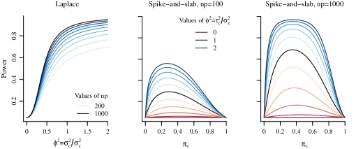
Figure 2: Approximate power of the test described in Proposition 3.1.

Now we consider the power for Bernoulli-normal distributed elements of $\boldsymbol{C}$.

Proposition 3.3

Assume that elements of $\boldsymbol{C}$ are independent, identically distributed Bernoulli-normal random variables. An element of $\boldsymbol{C}$ is exactly equal to zero with probability $1-\pi_{c}$, and normally distributed with mean zero and variance $\tau^{2}_{c}$ otherwise. Letting $\phi^{2}=\tau^{2}_{c}/\sigma^{2}_{z}$, as $n$ and $p\rightarrow\infty$, the asymptotic power of the test given by Proposition 3.1 is:

$$1-\Phi\left[\frac{z_{1-\alpha}-\pi_{c}\left(1-\pi_{c}\right)\left\{\sqrt{\frac{3np}{8}}\left(\frac{\phi^{2}}{\pi_{c}\phi^{2}+1}\right)^{2}\right\}}{\sqrt{1+\pi_{c}\left(1-\pi_{c}\right)\left\{\frac{\left(20\pi_{c}^{2}-28\pi_{c}+35\right)\phi^{8}+16\left(5-\pi_{c}\right)\phi^{6}+72\phi^{4}}{8\left(\pi_{c}\phi^{2}+1\right)^{4}}\right\}}}\right].$$

The approximate power depends on the variances of the nonzero effects $\tau^{2}_{c}$ and the noise $\sigma^{2}_{z}$ only through their ratio $\phi^{2}$. It is plotted for $\alpha=0.05$, $\pi_{c}\in\left[0,1\right]$, $\phi^{2}\in\left\{0,0.2,\dots,2\right\}$ and $np=\left\{100,1000\right\}$ in Figure 2. The approximate power is always increasing in $\phi^{2}$ and $np$. For fixed $\phi^{2}$ and $np$, power diminishes as the probability of an element of $\boldsymbol{C}$ being nonzero $\pi_{c}$ approaches $0$ or $1$ and $\boldsymbol{C}+\boldsymbol{Z}$ becomes more normally distributed. Overall, the test is more powerful when estimating $\boldsymbol{C}$ separately from $\boldsymbol{Z}$ is more valuable, e.g. when elements of $\boldsymbol{C}$ are large in magnitude relative to the noise and when many entries of $\boldsymbol{C}$ are exactly zero.

3.4 Robustness and Comparative Performance

If the true model is not the LANOVA model and elements of $\boldsymbol{C}$ are drawn from a different heavy-tailed distribution, it is natural to ask how our estimates $\widehat{\sigma}^{2}_{c}$, $\widehat{\sigma}^{2}_{z}$, and $\widehat{\boldsymbol{M}}$ perform. As $\boldsymbol{M}$ is a function of $\mu$, $\boldsymbol{a}$, $\boldsymbol{b}$ and $\boldsymbol{C}$, the performance of $\widehat{\boldsymbol{M}}$ also reflects the performance of $\widehat{\mu}$, $\widehat{\boldsymbol{a}}$, $\widehat{\boldsymbol{b}}$ and $\widehat{\boldsymbol{C}}$ indirectly. We find that the excess kurtosis $\kappa$ of the “true” distribution of elements of $\boldsymbol{C}$ determines our ability to estimate $\sigma^{2}_{c}$ separately from $\sigma^{2}_{z}$.

Proposition 3.4

Under the model $\boldsymbol{Y}=\mu\boldsymbol{1}_{n}\boldsymbol{1}_{p}^{\prime}+\boldsymbol{a}\boldsymbol{1}_{p}^{\prime}+\boldsymbol{1}_{n}\boldsymbol{b}^{\prime}+\boldsymbol{C}+\boldsymbol{Z}$, where elements of $\boldsymbol{C}$ are independent, identically distributed draws from a mean zero, symmetric distribution with variance $\sigma^{2}_{c}$, excess kurtosis $\kappa$ and finite eighth moment and elements of $\boldsymbol{Z}$ are normally distributed with mean zero and variance $\sigma^{2}_{z}$, $\widehat{\sigma}^{2}_{c}\stackrel{{\scriptstyle p}}{{\rightarrow}}\sqrt{\kappa/3}\sigma^{2}_{c}$ and $\widehat{\sigma}^{2}_{z}\stackrel{{\scriptstyle p}}{{\rightarrow}}\sigma^{2}_{z}+\left(1-\sqrt{\kappa/3}\right)\sigma^{2}_{c}$ as $n\rightarrow\infty$ with $p$ fixed, $p\rightarrow\infty$ with $n$ fixed, or $n$ and $p\rightarrow\infty$.

Proposition 3.4 indicates that we underestimate $\sigma^{2}_{c}$ when elements of $\boldsymbol{C}$ are lighter-than-Laplace tailed and we overestimate $\sigma^{2}_{c}$ when elements of $\boldsymbol{C}$ are heavier-than-Laplace tailed. To see how this affects estimation of $\boldsymbol{M}$, we consider exponential power and Bernoulli-normal distributed elements of $\boldsymbol{C}$. Exponential power distributed $c_{ij}$ have density $p(c_{ij}|\sigma^{2}_{c},q_{c})=(q_{c}/(2\sigma_{c}))\sqrt{\Gamma(3/q_{c})/\Gamma(1/q_{c})^{3}}\text{exp}\{-(\Gamma(3/q_{c})/\Gamma(1/q_{c}))^{q_{c}/2}|c_{ij}/\sigma_{c}|^{q_{c}}\}$ that is parameterized in terms of the variance $\sigma^{2}_{c}$ and a shape parameter $q_{c}$, and Bernoulli-normal distributed $c_{ij}$ are exactly equal to zero with probability $1-\pi_{c}$ and normally distributed with mean zero and $\tau^{2}_{c}$ otherwise. Both distributions can be lighter- or heavier-than-Laplace tailed. The excess kurtosis of exponential power and Bernoulli-normal $c_{ij}$ is $\Gamma\left(5/q_{c}\right)\Gamma\left(1/q_{c}\right)/\Gamma\left(3/q_{c}\right)^{2}-3$ and $3\left(1-\pi_{c}\right)/\pi_{c}$, respectively. As a result, elements of $\boldsymbol{C}$ will be heavier-than-Laplace tailed when $q_{c}<1$ or $\pi_{c}<0.5$ and lighter-than-Laplace tailed when $q_{c}>1$ or $\pi_{c}>0.5$. Note that when $q_{c}=1$ the exponential power distribution corresponds to the Laplace distribution and the LANOVA model is correct, and when $\pi_{c}=0.5$ the spike-and-slab distributed $\boldsymbol{C}$ have the same excess kurtosis as Laplace distributed $\boldsymbol{C}$ and the variance estimators $\widehat{\sigma}^{2}_{c}$ and $\widehat{\sigma}^{2}_{z}$ will be consistent.

We compare the risk of the LANOVA estimate $\widehat{\boldsymbol{M}}$ to the risk of the maximum likelihood estimate $\widehat{\boldsymbol{M}}_{MLE}$, the risk of the strictly additive estimate $\widehat{\boldsymbol{M}}_{ADD}$, the risk of additive-plus-low-rank estimates $\widehat{\boldsymbol{M}}_{LOW,1}$ and $\widehat{\boldsymbol{M}}_{LOW,5}$ which assume rank-one and rank-five $\boldsymbol{C}$ respectively, the risk of the soft- and hard-thresholding IPOD estimates of She and Owen (2011) $\widehat{\boldsymbol{M}}_{IPOD,S}$ and $\widehat{\boldsymbol{M}}_{IPOD,H}$, and the risk of approximately minimax estimates $\widehat{\boldsymbol{M}}_{MINI,U}$ and $\widehat{\boldsymbol{M}}_{MINI,S}$ obtained using the universal threshold and Stein’s unbiased risk estimate (SURE) described by Donoho and Johnstone (1994). Additive-plus-low-rank estimates are computed according to Johnson and Graybill (1972). Approximately minimax estimates are computed according to $\widehat{\boldsymbol{M}}_{MINI,U}=\widehat{\boldsymbol{M}}_{ADD}+\widehat{\boldsymbol{C}}_{MINI,U}$ and $\widehat{\boldsymbol{M}}_{MINI,S}=\widehat{\boldsymbol{M}}_{ADD}+\widehat{\boldsymbol{C}}_{MINI,S}$, where $\widehat{\boldsymbol{C}}_{MINI,S}$ and $\widehat{\boldsymbol{C}}_{MINI,S}$ are obtained by applying the universal threshold or SURE soft thresholding methods given by Donoho and Johnstone (1994) to elements of $\boldsymbol{Y}-\widehat{\boldsymbol{M}}_{ADD}$, as if elements of $\boldsymbol{Y}-\widehat{\boldsymbol{M}}_{ADD}$ were independent and identically distributed.

We compute Monte Carlo estimates of the relative risks for $n=p=25$, $\mu=0$, $\boldsymbol{a}=\boldsymbol{0}$, $\boldsymbol{b}=\boldsymbol{0}$ and $\sigma^{2}_{z}=1$. For exponential power distributed $\boldsymbol{C}$, we vary $\sigma^{2}_{c}=\left\{1/2,1,2\right\}$ and $q_{c}=\left\{0.1,\dots,1.9\right\}$. For Bernoulli-normal distributed $\boldsymbol{C}$, we vary $\tau^{2}_{c}=\left\{1/2,1,2\right\}$ and $\pi_{c}=\left\{0,0.1,\dots,0.9,1\right\}$. For each $(\sigma^{2}_{c},q_{c})$ and $(\tau^{2}_{c},\pi_{c})$, the Monte Carlo estimate is based on 500 simulated $\boldsymbol{Y}$.

The results shown in Figure 3 indicate generally favorable performance of the LANOVA estimate $\widehat{\boldsymbol{M}}$. The top four plots show log relative risk estimates when elements of $\boldsymbol{C}$ are exponential power distributed, whereas the bottom four plots show log relative risk estimates when elements of $\boldsymbol{C}$ are Bernoulli-normal distributed. As expected, the LANOVA estimate performs as well as or better than all alternative estimators when $q_{c}=1$ and the LANOVA model is true. Interestingly, the LANOVA estimate also performs as well as or better than all alternative estimators when $\pi_{c}=0.5$, even though the LANOVA model is not true. This suggests that the LANOVA estimate will tend to perform well relative to alternative estimators when the excess kurtosis of elements of $\boldsymbol{C}$ is similar to the excess kurtosis of a Laplace distribution. This is consistent with Proposition 3.4, which states that the asymptotic bias of the variance estimators $\widehat{\sigma}^{2}_{c}$ and $\widehat{\sigma}^{2}_{z}$ will depend on the excess kurtosis of the true distribution of elements of $\boldsymbol{C}$.

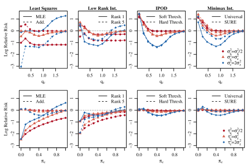
Figure 3: Monte Carlo approximations of the relative risks of the LANOVA estimate $\widehat{\boldsymbol{M}}$ versus the MLE $\widehat{\boldsymbol{M}}_{MLE}$, the strictly additive estimate of $\widehat{\boldsymbol{M}}_{ADD}$, additive-plus-low-rank estimates $\widehat{\boldsymbol{M}}_{LOW,1}$ and $\widehat{\boldsymbol{M}}_{LOW,5}$ based on rank-1 and rank-5 estimates of $\boldsymbol{C}$, soft- and hard-thresholding IPOD estimates $\widehat{\boldsymbol{M}}_{IPOD,S}$ and $\widehat{\boldsymbol{M}}_{IPOD,H}$, and universal threshold and SURE based approximately minimax estimates $\widehat{\boldsymbol{M}}_{MINI,U}$ and $\widehat{\boldsymbol{M}}_{MINI,S}$.

In the first column of Figure 3, we see that the LANOVA estimate $\widehat{\boldsymbol{M}}$ tends to outperform the strictly non-additive estimate $\widehat{\boldsymbol{M}}_{MLE}$ when $q_{c}<1$ or $\pi_{c}<0.5$, especially when the variance of the interactions $\sigma^{2}_{c}$ or $\tau^{2}_{c}$ is small relative to the variance of the noise $\sigma^{2}_{z}$. Intuitively, this makes sense. When $q_{c}$ is small we expect that many elements of $\boldsymbol{C}$ will be very close to zero, and when $\pi_{c}$ is small, many elements of $\boldsymbol{C}$ will be exactly equal to zero. Furthermore, when $\sigma^{2}_{c}$ or $\tau^{2}_{c}$ are small we expect even the largest interactions to be small relative to the noise. Accordingly, this suggests that $\widehat{\boldsymbol{M}}$ tends to outperform the strictly non-additive estimate $\widehat{\boldsymbol{M}}_{MLE}$ when $\boldsymbol{M}$ is more nearly additive. Analogously, the LANOVA estimate $\widehat{\boldsymbol{M}}$ tends to outperform the strictly additive estimate $\widehat{\boldsymbol{M}}_{ADD}$ when $q_{c}>1$ or $\pi_{c}>0.5$, especially when the variance of the interactions $\sigma^{2}_{c}$ or $\tau^{2}_{c}$ is large relative to the variance of the noise $\sigma^{2}_{z}$. Again, this makes sense because we expect that fewer elements of $\boldsymbol{C}$ will be nearly or exactly equal to zero when $q_{c}>1$ or $\pi_{c}>0.5$, and more elements of $\boldsymbol{M}$ will be strictly non-additive.

In the second column of Figure 3, we see that the relative performance of the LANOVA estimate $\widehat{\boldsymbol{M}}$ relative to the additive-plus-low-rank estimates $\widehat{\boldsymbol{M}}_{LOW,1}$ and $\widehat{\boldsymbol{M}}_{LOW,5}$ depends on the distribution of elements of $\boldsymbol{C}$. When elements of $\boldsymbol{C}$ are exponential power distributed, the LANOVA estimate $\widehat{\boldsymbol{M}}$ outperforms the additive-plus-low-rank estimates $\widehat{\boldsymbol{M}}_{LOW,1}$ and $\widehat{\boldsymbol{M}}_{LOW,5}$ as long as $q_{c}$ is neither to small nor too large, especially when the variance of the interactions $\sigma^{2}_{c}$ is large relative to the variance of the noise $\sigma^{2}_{z}$. When elements of $\boldsymbol{C}$ are Bernoulli-normal distributed, the LANOVA estimate $\widehat{\boldsymbol{M}}$ almost always outperforms both additive-plus-low-rank estimates $\widehat{\boldsymbol{M}}_{LOW,1}$ and $\widehat{\boldsymbol{M}}_{LOW,5}$. This makes sense, as low rank approximations of sparse matrices tend to perform poorly.

In the third column, we see that the LANOVA estimate $\widehat{\boldsymbol{M}}$ tends to outperform the the soft- and hard-thresholding IPOD estimates $\widehat{\boldsymbol{M}}_{IPOD,S}$ and $\widehat{\boldsymbol{M}}_{IPOD,H}$ for values of $q_{c}>0.5$ and all values of $\pi_{c}$ and $\tau^{2}_{c}$. The soft-thresholding IPOD estimate $\widehat{\boldsymbol{M}}_{IPOD,S}$ performs almost identically to the strictly additive estimate $\widehat{\boldsymbol{M}}_{ADD}$ which suggests that it tends to overpenalize elements of $\boldsymbol{C}$. Surprisingly, $\widehat{\boldsymbol{M}}_{IPOD,S}$ tends to slightly outperform $\widehat{\boldsymbol{M}}_{IPOD,H}$. As discussed in She and Owen (2011), outlier detection based on convex penalties, which are used to compute $\widehat{\boldsymbol{M}}$ and $\widehat{\boldsymbol{M}}_{IPOD,S}$, tends to perform worse than outlier detection based on nonconvex penalties, which are used to compute $\widehat{\boldsymbol{M}}_{IPOD,H}$. However the relatively better performance of $\widehat{\boldsymbol{M}}$ and $\widehat{\boldsymbol{M}}_{IPOD,S}$ relative to $\widehat{\boldsymbol{M}}_{IPOD,H}$ can be attributed to the fact that outlier detection based on convex penalties performs well when all observations have equal leverage, as is the case in this setting (Rousseeuw and Leroy, 1987). The LANOVA estimate $\hat{\boldsymbol{M}}$ is also much faster to compute than both IPOD estimates; the soft- and hard-thresholding IPOD estimates take over $1,000$ times longer than the LANOVA estimate to compute on average across all simulations.

In the last column, we see that the LANOVA estimate $\widehat{\boldsymbol{M}}$ tends to outperform the approximately minimax estimates $\widehat{\boldsymbol{M}}_{MINI,U}$ and $\widehat{\boldsymbol{M}}_{MINI,S}$ as long as elements of $\boldsymbol{C}$ are not extremely heavy tailed or extremely sparse, especially when the variance of the interactions $\sigma^{2}_{c}$ is large relative to the variance of the noise $\sigma^{2}_{z}$. Additionally, the improvements offered by the LANOVA estimate $\widehat{\boldsymbol{M}}$ over the approximately minimax estimates $\widehat{\boldsymbol{M}}_{MINI,U}$ and $\widehat{\boldsymbol{M}}_{MINI,S}$ are greater when $\boldsymbol{C}$ is exponential power distributed versus Bernoulli-normal distributed, which suggests that LANOVA penalization may be particularly useful when we expect that some elements of $\boldsymbol{C}$ are nearly but not exactly equal to zero.

Altogether, these results also suggest that the LANOVA estimate $\widehat{\boldsymbol{M}}$ can offer better or comparable performance relative to alternatives as long as the tail behavior of elements of $\boldsymbol{C}$ is not too different from the tail behavior of a Laplace distribution. Relatedly, the results also also suggest that we might be able to construct an improved estimate of $\boldsymbol{M}$ based on LANOVA penalization if prior information on the tail behavior of elements of $\boldsymbol{C}$ is available. The results displayed in Figure 3 suggest that the biased estimation of $\widehat{\sigma}^{2}_{c}$ and $\widehat{\sigma}^{2}_{z}$ when elements of $\boldsymbol{C}$ have lighter- or heavier-than Laplace tailed described in Proposition 3.4 leads to poorer LANOVA estimates of $\boldsymbol{M}$. Fortunately, this suggests that estimation of $\boldsymbol{M}$ could be improved if less biased estimates of $\widehat{\sigma}^{2}_{c}$ and $\widehat{\sigma}^{2}_{z}$ could be obtained. Proposition 3.4 suggests a correction of multiplying $\widehat{\sigma}^{2}_{c}$ by $\sqrt{3/\kappa}$ and subtracting $(1-\sqrt{\kappa/3})\sqrt{3/\kappa}\widehat{\sigma}^{2}_{c}$ from $\widehat{\sigma}^{2}_{z}$. However because excess kurtosis $\kappa$ is not a readily interpretable quantity, specifying a more appropriate value of $\kappa$ a priori may be difficult. However if a Bernoulli-normal distribution for elements of $\boldsymbol{C}$ is plausible, a more appropriate value of $\pi_{c}$ can be used to specify a more appropriate value of $\kappa$. If the new value of $\pi_{c}$ is close to the “true” proportion of nonzero elements of $\boldsymbol{C}$, this may improve estimation of $\sigma^{2}_{c}$ and $\sigma^{2}_{z}$ and accordingly, $\boldsymbol{M}$.

4 Extensions

4.1 Penalizing Lower-Order Parameters

When $\boldsymbol{Y}$ has many rows or columns, it may be reasonable to believe that many elements of $\boldsymbol{a}$ or $\boldsymbol{b}$ are exactly zero. A natural extension of Equation (2) is given by

$$\text{min}_{\mu,\boldsymbol{a},\boldsymbol{b},\boldsymbol{C}}\frac{1}{2\sigma^{2}_{z}}\left|\left|\text{vec}\left(\boldsymbol{Y}-\boldsymbol{M}\right)\right|\right|^{2}_{2}+\lambda_{a}\left|\left|\boldsymbol{a}\right|\right|_{1}+\lambda_{b}\left|\left|\boldsymbol{b}\right|\right|_{1}+\lambda_{c}\left|\left|\text{vec}\left(\boldsymbol{C}\right)\right|\right|_{1},$$ (5)

where we still have $\boldsymbol{M}=\boldsymbol{1}_{n}\boldsymbol{1}_{p}^{\prime}\mu+\boldsymbol{a}\boldsymbol{1}_{p}^{\prime}+\boldsymbol{1}_{n}\boldsymbol{b}^{\prime}+\boldsymbol{C}$. Again, using the posterior mode interpretation of Equation (5), we can estimate $\sigma^{2}_{a}$ and $\sigma^{2}_{b}$ from the observed data, $\boldsymbol{Y}$:

$$\widehat{\sigma}^{2}_{a} =\frac{1}{n-1}\sum_{i=1}^{n}\check{a}^{2}_{i}-\frac{n}{\left(n-1\right)\left(p-1\right)}\overline{r}^{\left(2\right)}\text{, \quad}\widehat{\sigma}^{2}_{b}=\frac{1}{p-1}\sum_{j=1}^{p}\check{b}^{2}_{j}-\frac{p}{\left(n-1\right)\left(p-1\right)}\overline{r}^{\left(2\right)}.$$

where $\check{\boldsymbol{a}}=\boldsymbol{H}_{n}\boldsymbol{Y}\boldsymbol{1}_{p}/p$ and $\check{\boldsymbol{b}}=\boldsymbol{H}_{p}\boldsymbol{Y}^{\prime}\boldsymbol{1}_{n}/n$ are OLS estimates for $\boldsymbol{a}$ and $\boldsymbol{b}$. The estimators $\widehat{\lambda}_{a}=\sqrt{2/\widehat{\sigma}^{2}_{a}}$ and $\widehat{\lambda}_{b}=\sqrt{2/{\widehat{\sigma}^{2}_{b}}}$ can be shown to be consistent for $\lambda_{a}$ and $\lambda_{b}$ as $n\rightarrow\infty$ and $p\rightarrow\infty$, respectively. Because $\widehat{\lambda}_{c}$ and $\widehat{\sigma}^{2}_{z}$ do not depend on of $\boldsymbol{a}$ and $\boldsymbol{b}$, our estimators for $\lambda_{c}$ and $\sigma^{2}_{z}$ are unchanged. A block coordinate descent algorithm for solving Equation (5) is given in the web appendix. With respect to interpretation, population average row and column main effects can be obtained via ANOVA decomposition of $\widehat{\boldsymbol{M}}$.

4.2 Tensor Data

LANOVA penalization can be extended to a $p_{1}\times p_{2}\times\dots\times p_{K}$ $K$-mode tensor $\boldsymbol{Y}$. We consider:

$$\text{vec}\left(\boldsymbol{Y}\right) =\boldsymbol{W}\boldsymbol{\beta}+\text{vec}\left(\boldsymbol{C}\right)+\text{vec}\left(\boldsymbol{Z}\right),$$ (6)

$$\boldsymbol{C} =\left\{c_{i_{1}\dots i_{K}}\right\}\sim\text{i.i.d. Laplace}\left(0,\lambda_{c}^{-1}\right)\text{, \quad}\boldsymbol{Z}=\left\{z_{i_{1}\dots i_{K}}\right\}\sim\text{i.i.d. N}\left(0,\sigma^{2}_{z}\right),$$

where $\text{vec}\left(\boldsymbol{Y}\right)$ is the $\prod_{k=1}^{K}p_{k}\times 1$ vectorization of the $K$-mode tensor $\boldsymbol{Y}$ with “lower” indices moving “faster” and $\boldsymbol{W}$ and $\boldsymbol{\beta}$ are the design matrix and unknown mean parameters corresponding to a $K$-way ANOVA decomposition treating the $K$ modes of $\boldsymbol{Y}$ as factors. The matrix $\boldsymbol{W}=\left[\boldsymbol{W}_{1},\dots,\boldsymbol{W}_{2^{K}-1}\right]$ is obtained by concatenating the $2^{K}-1$ unique matrices of the form $\boldsymbol{W}_{l}=\left(\boldsymbol{W}_{l,1}\otimes\dots\otimes\boldsymbol{W}_{l,K}\right)$, where each $\boldsymbol{W}_{l,k}$ is equal to either $\boldsymbol{I}_{p_{k}}$ or $\boldsymbol{1}_{p_{k}}$, excluding the identity matrix, $\boldsymbol{I}_{p_{K}}\otimes\dots\otimes\boldsymbol{I}_{p_{1}}$. As in the matrix case, approaches that assume a low rank $\boldsymbol{C}$ are common (van Eeuwijk and Kroonenberg, 1998; Gerard and Hoff, 2017). We penalize elements of the highest order mean term $\boldsymbol{C}$ for which no replicates are observed. In the three-way tensor case, the first part of Equation (6) refers to the following decomposition:

$$y_{ijk}=\mu+a_{i}+b_{j}+d_{k}+e_{ij}+f_{ik}+g_{jk}+c_{ijk}+z_{ijk}.$$ (7)

Estimates of $\sigma^{2}_{z}$ and $\lambda_{c}$ are constructed from $\text{vec}\left(\boldsymbol{R}\right)=\left(\boldsymbol{H}_{K}\otimes\dots\otimes\boldsymbol{H}_{1}\right)\text{vec}\left(\boldsymbol{Y}\right)$, where $\boldsymbol{H}_{k}=\boldsymbol{I}_{p_{k}}-\boldsymbol{1}_{p_{k}}\boldsymbol{1}_{p_{k}}/p_{k}$ is the $p_{k}\times p_{k}$ centering matrix and ‘$\otimes$’ is the Kronecker product. As in the matrix case, $\text{vec}\left(\boldsymbol{R}\right)$ is independent of the lower-order unknown mean parameters $\boldsymbol{\beta}$, i.e. $\text{vec}\left(\boldsymbol{R}\right)=\left(\boldsymbol{H}_{K}\otimes\dots\otimes\boldsymbol{H}_{1}\right)\text{vec}\left(\boldsymbol{C}+\boldsymbol{Z}\right)$. Our estimates of $\sigma^{2}_{z}$ and $\lambda_{c}$ are still functions of the second and fourth sample moments of $\boldsymbol{R}$: $\overline{r}^{\left(2\right)}=\frac{1}{p}\sum_{i=1}^{p}r^{2}_{i}$ and $\overline{r}^{\left(4\right)}=\frac{1}{p}\sum_{i=1}^{p}r^{4}_{i}$, where $p=\prod_{k=1}^{K}p_{k}$. We extend our empirical Bayes estimators as follows:

$$\widehat{\sigma}^{4}_{c}= \left\{\prod_{k=1}^{K}\frac{p_{k}^{3}}{\left(p_{k}-1\right)\left(p_{k}^{2}-3p_{k}+3\right)}\right\}\left\{\overline{r}^{\left(4\right)}/3-\left(\overline{r}^{\left(2\right)}\right)^{2}\right\},$$ (8)

$$\widehat{\sigma}^{2}_{c}= \sqrt{\widehat{\sigma}^{4}_{c}}\text{,\quad}\widehat{\sigma}^{2}_{z}=\left(\prod_{k=1}^{K}\frac{p_{k}}{p_{k}-1}\right)\overline{r}^{\left(2\right)}-\widehat{\sigma}^{2}_{c},$$

where $\widehat{\lambda}_{c}=\sqrt{2/\widehat{\sigma}^{2}_{c}}$. As in the matrix case, we can compute the bias of $\widehat{\sigma}^{4}_{c}$.

Proposition 4.1

Under the model given by Equation (6),

$$\mathbb{E}\left[\widehat{\sigma}^{4}_{c}\right]-\sigma^{4}_{c}= -\left\{\prod_{k=1}^{K}\frac{p_{k}^{3}}{\left(p_{k}-1\right)\left(p^{2}_{k}-3p_{k}+3\right)}\right\}\left[\left\{3\prod_{k=1}^{K}\frac{\left(p_{k}-1\right)^{2}}{p_{k}^{3}}\right\}\sigma^{4}_{c}+\right.$$

$$\left.\left(2\prod_{k=1}^{K}\frac{p_{k}-1}{p_{k}^{2}}\right)\left(\sigma^{2}_{c}+\sigma^{2}_{z}\right)^{2}\right].$$

Interpretation of this result is analogous to the matrix case. We tend to prefer the simpler model with $\text{vec}\left(\boldsymbol{C}\right)=\boldsymbol{0}$ over a more complicated model with nonzero elements of $\text{vec}\left(\boldsymbol{C}\right)$ when few data are available or when the data is very noisy. Additionally, $\mathbb{E}\left[\widehat{\sigma}^{4}_{c}\right]-\sigma^{4}_{c}=O\left(1/p\right)$, i.e. the bias of $\widehat{\sigma}^{4}_{c}$ diminishes as the number of levels of any mode increases. We also assess the large-sample performance of our empirical Bayes estimators in the $K$-way tensor case.

Proposition 4.2

Under the model given by Equation (6), $\widehat{\sigma}^{4}_{c}\stackrel{{\scriptstyle p}}{{\rightarrow}}\sigma^{4}_{c}$, $\widehat{\sigma}^{2}_{c}\stackrel{{\scriptstyle p}}{{\rightarrow}}\sigma^{2}_{c}$, $\widehat{\lambda}_{c}\stackrel{{\scriptstyle p}}{{\rightarrow}}\lambda_{c}$ and $\widehat{\sigma}^{2}_{z}\stackrel{{\scriptstyle p}}{{\rightarrow}}\sigma^{2}_{z}$ as $p_{k^{\prime}}\rightarrow\infty$ with $p_{k}$, $k\neq k^{\prime}$, fixed or $p_{1},\dots,p_{K}\rightarrow\infty$.

A block coordinate descent algorithm for estimating the unknown mean parameters is given in the web appendix. Results for testing the appropriateness of assuming heavy-tailed $\boldsymbol{C}$ and robustness carry over to $K$-way tensors. $K$-way tensor analogues to Propositions 3.1-3.4, where we replace $np$ with $p$ and assume all $p_{1},\dots,p_{K}\rightarrow\infty$, are shown to hold in the web appendix. Lastly we can also extend LANOVA penalization for tensor data to penalize lower-order mean parameters. Because tensor-variate $\boldsymbol{Y}$ include even more lower-order mean parameters, penalizing lower-order parameters is especially useful. We give nuisance parameter estimators for penalizing lower-order parameters in the three-way case in the web appendix.

5 Numerical Examples

Brain Tumor Data:

We consider a $356\times 43$ matrix of gene expression measurements for 356 genes and 43 brain tumors. The 43 brain tumors include 24 glioblastomas and 19 oligodendrogal tumors, which include 5 astrocytomas, 8 oliodendrogliomas and 6 mixed oligoastrocytomas. This data is contained in the denoiseR package for R (Josse et al., 2016), and it has been used to identify genes associated with glioblastomas versus oligodendrogal tumors (Bredel et al., 2005; de Tayrac et al., 2009). We focus on comparison to de Tayrac et al. (2009), who used a variation of principal components analysis of $\boldsymbol{Y}$ to identify differentially expressed genes and groups of tumors which is similar to using an additive-plus-low-rank estimate of $\boldsymbol{M}$. To ensure a straightforward comparison to the methods used in de Tayrac et al. (2009), we do not perform any additional preprocessing of the data, e.g. adjustments for possible low rank confounding factors that are often observed in gene expression data (Leek and Storey, 2007; Gagnon-Bartsch et al., 2013).

Unlike pairwise test-based methods which require prespecified tumor groupings, LANOVA penalization and additive-plus-low-rank estimates can be used to examine differential expression both within and across types of brain tumors. Differential expression within types of brain tumors in particular is of recent interest (Bleeker et al., 2012).

We apply LANOVA penalization with penalized interaction effects and unpenalized main effects. The test given by Proposition 3.1 supports a non-additive estimate of $\boldsymbol{M}$; we obtain a test statistic of $18.45$ and reject the null hypothesis of normally distributed elementwise variability at level $\alpha=0.05$ with $p<10^{-5}$. We estimate that $11,188$ elements of $\boldsymbol{C}$ (73%) are exactly equal to zero, i.e. most genes are not differentially expressed. Figure 4 shows $\widehat{\boldsymbol{C}}$ and a subset containing fifty genes with the lowest gene-by-tumor sparsity rates.

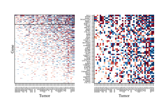
Figure 4: Elements of the $356\times 43$ matrix $\widehat{\boldsymbol{C}}$. The first panel shows the entire matrix $\widehat{\boldsymbol{C}}$ with rows (genes) and columns (tumors) sorted in decreasing order of the row and column sparsity rates. The second panel zooms in on the rows of $\widehat{\boldsymbol{C}}$ (genes) marked in the first panel, which correspond to the fifty rows (genes) with the lowest sparsity rates. Colors correspond to positive (red) versus negative (blue) values of $\widehat{\boldsymbol{C}}$ and darkness corresponds to magnitude.

The results of LANOVA penalization are consistent with those of de Tayrac et al. (2009). We observe that 49% and 56% of the elements of $\widehat{\boldsymbol{C}}$ involving the genes ASPA and PDPN are nonzero. Examination of $\widehat{\boldsymbol{M}}$ indicates overexpression of these genes among glioblastomas relative to oligodendrogal tumors, as observed in de Tayrac et al. (2009). LANOVA penalization yields additional results that are consistent with the wider literature. The gene DLL3 has the highest rate of gene-by-tumor interactions at 74% and tends to be underexpressed in glioblastomas. This is consistent with findings of overexpression of DLL3 in brain tumors with better prognoses (Bleeker et al., 2012). The KLRC genes KLRC1, KLRC2 and KLRC3.1 all have very high rates of gene-by-tumor interactions at 72%, 70% and 60%. Ducray et al. (2008) has found evidence for differential KLRC expression across glioma subtypes. LANOVA penalization also indicates that several brain tumors have unique gene expression profiles. Glioblastomas 3, 4 and 30 have rates of nonzero gene-by-tumor interactions exceeding 50% and similar gene expression profiles. Specifically, we observe overexpression of FCGR2B and HMOX1 and underexpression of RTN3 for gliomastomas 3, 4 and 30. Overexpression of FCGR2B or HMOX1 is associated with poorer prognosis (Zhang et al., 2016; Ghosh et al., 2016), and RTN3 is differentially expressed across subgroups of glioblastoma that differ with respect to prognosis (Cosset et al., 2017). This suggests that glioblastomas 3, 4 and 30 may correspond to an especially aggressive subtype.

fMRI Data:

Second, we consider a tensor of fMRI data which appeared in Mitchell et al. (2004). During each of 36 tasks, fMRI activations were measured at $55$ time points and $4,698$ locations (voxels). Accordingly, the data can be represented as a $36\times 55\times 4,698$ three-way tensor. Because the data is so high dimensional, many methods of analysis are prohibitively computationally burdensome. Accordingly, parcellation approaches that reduce the spatial resolution of fMRI data by grouping voxels into spatially contiguous groups are common, however, the choice of a specific parcellation can be difficult (Thirion et al., 2014). Instead, we propose LANOVA penalization as an exploratory method to identify relevant dimensions of spatial variation that should be accounted for in a subsequent analysis.

The test given by Proposition 3.1 supports a non-additive estimate of $\boldsymbol{M}$; we obtain a test statistic of $298.87$ and reject the null hypothesis of normally distributed elementwise variability at level $\alpha=0.05$ with $p<10^{-5}$. Having found support for the use of a non-additive estimate of $\boldsymbol{M}$, we also penalize lower-order mean parameters as $\boldsymbol{Y}$ is high dimensional and sparsity of lower-order mean parameters could result in substantial dimension reduction and improved interpretability. The LANOVA estimate has $1,751,179$ nonzero parameters, a small fraction of the $9,302,040$ parameters needed to represent the raw data, $\boldsymbol{Y}$ ($18.83\%$).

Recalling that we are primarily interested in spatial variation, we examine estimated task-by-location interactions $\widehat{\boldsymbol{F}}$ and task-by-time-by-location elementwise interactions $\widehat{\boldsymbol{C}}$, as defined in Equation (7). Figure 5 shows the percent of nonzero entries $\widehat{\boldsymbol{F}}$ and $\widehat{\boldsymbol{C}}$ at each location. At each location, the proportion of nonzero entries of $\widehat{\boldsymbol{F}}$ is much larger than the proportion of nonzero entries of $\widehat{\boldsymbol{C}}$. This suggests that much of the spatial variation of activations by task can be attributed to an overall level change in activation over the duration of the task, as opposed to time-specific changes in activation. In a subsequent analysis, it may be reasonable to ignore task-by-time-by-location interactions.

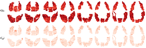
Figure 5: Percent of nonzero entries of $\widehat{\boldsymbol{F}}$ and $\widehat{\boldsymbol{C}}$ by location, where $\widehat{\boldsymbol{F}}$ and $\widehat{\boldsymbol{C}}$ estimate $\boldsymbol{F}$ and $\boldsymbol{C}$ as defined in Equation (7). Entries of $\boldsymbol{F}$ index task-by-location interaction terms and entries of $\boldsymbol{C}$ index task-by-time-by-location elementwise interaction terms. Darker colors indicate higher percentages.

By examining the percent of nonzero entries of $\widehat{\boldsymbol{F}}$ by location, we can get a sense of which locations correspond to level changes in fMRI activity response by task. There is evidence for an overall level change in response to at least some tasks for all locations; the minimum percent of nonzero entries of $\widehat{\boldsymbol{F}}$ per location is $33\%$. However, voxels in the the parietal region, the calcarine fissure and the right- and left-dorsolateral prefrontal cortex have particularly high proportions of nonzero entries of $\widehat{\boldsymbol{F}}$, suggesting that overall activation in these regions is particularly responsive to tasks. By examining the percent of nonzero entries of $\widehat{\boldsymbol{C}}$ by location, we can get a sense of which locations correspond to time-specific differential activity by task over time. We see that nonzero entries of $\widehat{\boldsymbol{C}}$ are concentrated among voxels in the upper supplementary motor area, the calcarine fissure and the left- and right-temporal lobes. In this way, we can use LANOVA estimates to identify subsets of relevant voxels that should be included in a subsequent analysis.

Fusarium Data:

Last, we consider the problem of checking for nonzero three-way interactions in experimental data without replicates. The data is a $20\times 7\times 4$ three-way tensor containing severity of disease incidence ratings for 20 varieties of wheat infected with 7 strains of Fusarium head blight over 4 years, from 1990-1993 that appeared in van Eeuwijk and Kroonenberg (1998). There is scientific reason to believe that several nonzero three-way variety-by-strain-by-year interactions are present. van Eeuwijk and Kroonenberg (1998) examined these interactions using a rank-one tensor model for $\boldsymbol{C}$, i.e. $c_{ijk}=\alpha_{i}\gamma_{j}\delta_{k}$. However as noted in Section 1, a low rank model may not be sufficient even if few nonzero interactions are present.

As in van Eeuwijk and Kroonenberg (1998), we transform the severity ratings to the logit scale before estimating LANOVA parameters. The test given by Proposition 3.1 supports a non-additive estimate of $\boldsymbol{M}$; we obtain a test statistic of $3.99$ and reject the null hypothesis of normally distributed elementwise variability at level $\alpha=0.05$ with $p=3.34\times 10^{-5}$. We obtain 87 nonzero entries of $\widehat{\boldsymbol{C}}$ ($16\%$).

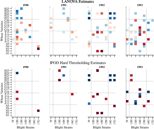
Figure 6: Entries of $\widehat{\boldsymbol{C}}$. Red (blue) points indicate positive (negative) nonzero entries of $\widehat{\boldsymbol{C}}$ and darker colors correspond to larger magnitudes.

Figure 6 shows nonzero elements of $\widehat{\boldsymbol{C}}$ as well as nonzero elements of $\widehat{\boldsymbol{C}}_{IPOD,H}$ obtained using the hard-thresholding IPOD method of She and Owen (2011), with dashed lines separating groups of wheat and blight by country of origin: Hungary (H), Germany (G), France (F) or the Netherlands (N). Estimates of elements of $\widehat{\boldsymbol{C}}_{IPOD,S}$ obtained using the soft-thresholding IPOD method of She and Owen (2011) are not pictured because they are all exactly equal to zero. We can interpret nonzero elements of estimates of $\boldsymbol{C}$ as evidence for variety-by-year-by-strain interactions that cannot be expressed as additive in variety-by-year, year-by-strain and variety-by-strain effects. Like van Eeuwijk and Kroonenberg (1998), both the LANOVA estimate $\widehat{C}$ and the hard-thresholding IPOD estimate $\widehat{\boldsymbol{C}}_{IPOD,H}$ include large three-way interactions in 1992, during which there was a disturbance in the storage of blight strains. Specifically, we observe interactions involving Dutch variety 2, the only variety with no infections at all in 1992, and interactions between Hungarian varieties 21 and 23 and foreign blight strains, which despite the storage disturbance were still able to cause infection in these two Hungarian varieties alone. The soft-thresholding IPOD estimate $\widehat{\boldsymbol{C}}_{IPOD,S}$ fails to include these real interactions, suggesting that it overpenalized $\boldsymbol{C}$ just as we observed in simulations. We do not have enough information about the data to assess whether or not the remaining interactions identified by $\hat{\boldsymbol{C}}$ and $\hat{\boldsymbol{C}}_{IPOD,H}$ are related to features of the study or known patterns in the behavior of certain varieties and strains, however they suggest further investigation of these varieties and strains may be warranted.

6 Discussion

This paper demonstrates the use the common Lasso penalty and the corresponding Laplace prior distribution for estimating elementwise effects of scientific interest in the absence of replicates. Our procedure, LANOVA penalization, can also be interpreted as assessing evidence for nonadditivity. We show that our nuisance parameter estimators are consistent and explore their behavior when assumptions are violated. We demonstrate that the corresponding mean parameter estimates can perform favorably relative to strictly additive, strictly non-additive, additive-plus-low-rank, IPOD, and approximately minimax estimates when elements of $\boldsymbol{C}$ are exponential power or Bernoulli-normal distributed, especially if the tail behavior of elements of $\boldsymbol{C}$ is similar to the tail behavior of a Laplace distribution and the variance of the interactions $\sigma^{2}_{c}$ is large relative to the variance of the noise $\sigma^{2}_{z}$. We emphasize that LANOVA penalization is computationally simple. The nuisance parameter estimators are easy to compute for arbitrarily large matrices and estimates of $\boldsymbol{M}$ can be computed using fast a block coordinate descent algorithm that exploits the structure of the problem. We also extend LANOVA penalization to penalize lower-order mean parameters and apply to tensors. Finally, we show that LANOVA estimates can be used to examine gene-by-tumor interactions using microarray data, to perform exploratory analysis of spatial variation in activation response to tasks over time in high dimensional fMRI data and to assess evidence for “real” elementwise interaction effects at in experimental data. To conclude, we discuss several limitations and extensions.

One limitation is that we assume heavy-tailed elementwise variation is of scientific interest and should be incorporated into the mean $\boldsymbol{M}$, whereas normally distributed elementwise variation is spurious noise $\boldsymbol{Z}$. If the noise is heavy-tailed, it may erroneously be incorporated into the estimate of $\boldsymbol{C}$. Similar issues arise with low rank models for $\boldsymbol{C}$, insofar as systematic correlated noise can erroneously be incorporated into the estimate of $\boldsymbol{C}$. Furthermore, if the elementwise variation of scientific interest includes low rank components, these low rank components may not be included in LANOVA estimates of the mean $\boldsymbol{M}$. This is of particular concern in the brain tumor data example but also of more general concern in applications involving gene expression data, because unobserved confounders with low rank structure may be present and need to be accounted for (Leek and Storey, 2007; Gagnon-Bartsch et al., 2013). That said, any method that aims to separate elementwise variation into components that are of scientific interest and spurious noise requires strong assumptions that must be considered in the context of the problem.

Another limitation is that the results of the simulation study assessing the performance of the LANOVA estimate $\widehat{\boldsymbol{M}}$ do not necessarily suggest favorable performance of the LANOVA estimate in all settings. First, we only consider exponential power and Bernoulli-normal elements of $\boldsymbol{C}$. Although we expect the LANOVA estimate to perform well when elements of $\boldsymbol{C}$ are heavy tailed, we do not expect the LANOVA estimate to perform well when $\boldsymbol{C}$ are light-tailed. Second, this scenario considers $\boldsymbol{C}$ with independent, identically distributed elements. In some settings, it may be reasonable to expect dependence across elements of $\boldsymbol{C}$ and additive-plus-low-rank estimates may perform better.

The methods presented in this paper could be extended in several ways. Although we use our estimators of $\lambda_{c}$ and $\sigma^{2}_{z}$ in posterior mode estimation, the same estimators could also be used to simulate from the posterior distribution using a Gibbs sampler. The output of a Gibbs sampler could be used to construct credible intervals for elements of $\boldsymbol{M}$, which would be one way of addressing uncertainty. We may also want to account for additional uncertainty induced by estimating $\lambda_{c}$ and $\sigma^{2}_{z}$. To address this, a fully Bayesian approach with prior distributions set for $\lambda_{c}$ and $\sigma^{2}_{z}$ could be taken at the cost of losing a sparse estimate of $\boldsymbol{C}$. Our empirical Bayes nuisance parameter estimators could be used to set parameters of prior distributions for $\lambda_{c}$ or $\sigma^{2}_{z}$. Last, LANOVA penalization for matrices is a specific case of the more general bilinear regression model, where we assume $\boldsymbol{Y}=\boldsymbol{A}\boldsymbol{W}+\boldsymbol{B}\boldsymbol{X}+\boldsymbol{C}+\boldsymbol{Z}$, given known $\boldsymbol{W}$ and $\boldsymbol{X}$. We chose to focus on a simpler case in this paper to facilitate the derivation of interpretable expressions for the bias of $\sigma^{4}_{c}$ as well as estimators that are consistent as either $n$ or $p\rightarrow\infty$ because researchers often encounter “fat” or “skinny” matrices in practice. However, the same logic could easily be extended to the more general bilinear regression context as well as the even more general multilinear context for tensor $\boldsymbol{Y}$.

Finally, our intuition combined with the results of Section 3 suggests that the Laplace distributional assumptions used in this paper are likely to be violated in many settings. The strength of the Laplace distributional assumption for elements of $\boldsymbol{C}$ can be justified by the need to make some assumptions to estimate $\sigma^{2}_{c}$ and $\sigma^{2}_{z}$ when $\boldsymbol{C}$ and $\boldsymbol{Z}$ are always observed as a sum $\boldsymbol{C}+\boldsymbol{Z}$. Given that we need to estimate fourth order moments of $\boldsymbol{C}$ and $\boldsymbol{Z}$ just to separately estimate $\sigma^{2}_{c}$ and $\sigma^{2}_{z}$, we expect that we would need to estimate even higher order moments to assess the appropriateness of the Laplace distributional assumption for $\boldsymbol{C}$ which is notoriously difficult to do well in practice. However, if we observed replicate measurements, as is the case for lower-order mean parameters $\boldsymbol{a}$ and $\boldsymbol{b}$, we would not need to estimate fourth order moments to separately estimate $\sigma^{2}_{a}$ or $\sigma^{2}_{b}$ from $\sigma^{2}_{z}$. Instead, we could use fourth order moments to assess the appropriateness of the Laplace distributional assumptions for $\boldsymbol{a}$ or $\boldsymbol{b}$ and possibly improve distribution specification. In recent work, we have considered this question in the general regression setting and have found that it can be possible to test the appropriateness of Laplace distributional assumptions and, when Laplace distributional assumptions are inappropriate, choose better ones (Griffin and Hoff, 2017).

References

- Bleeker et al. (2012) Bleeker, F. E., R. J. Molenaar, and S. Leenstra (2012). Recent advances in the molecular understanding of glioblastoma. Journal of Neuro-Oncology 108(1), 11–27.
- Bredel et al. (2005) Bredel, M., C. Bredel, D. Juric, G. R. Harsh, H. Vogel, L. D. Recht, and B. I. Sikic (2005). Functional Network Analysis Reveals Extended Gliomagenesis Pathway Maps and Three Novel MYC-Interacting Genes in Human Gliomas. Cancer Research 65(19), 8679–8689.
- Cosset et al. (2017) Cosset, É., S. Ilmjärv, V. Dutoit, K. Elliott, T. von Schalscha, M. F. Camargo, A. Reiss, T. Moroishi, L. Seguin, G. Gomez, J. S. Moo, O. Preynat-Seauve, K. H. Krause, H. Chneiweiss, J. N. Sarkaria, K. L. Guan, P. Y. Dietrich, S. M. Weis, P. S. Mischel, and D. A. Cheresh (2017). Glut3 Addiction Is a Druggable Vulnerability for a Molecularly Defined Subpopulation of Glioblastoma. Cancer Cell 32, 856–868.
- de Tayrac et al. (2009) de Tayrac, M., S. Lê, M. Aubry, J. Mosser, and F. Husson (2009). Simultaneous analysis of distinct Omics data sets with integration of biological knowledge: Multiple Factor Analysis approach. BMC Genomics 10(1), 32.
- Díaz-Francés and Montoya (2008) Díaz-Francés, E. and J. A. Montoya (2008). Correction to “On the linear combination of normal and Laplace random variables”, by Nadarajah, S., Computational Statistics, 2006, 21, 63–71. Computational Statistics 23(4), 661–666.
- Donoho and Johnstone (1994) Donoho, D. L. and I. M. Johnstone (1994). Ideal spatial adaptation by wavelet shrinkage. Biometrika 81(July), 425–455.
- Donoho and Johnstone (1995) Donoho, D. L. and I. M. Johnstone (1995). Adapting to Unknown Smoothness via Wavelet Shrinkage. Journal of the American Statistical Association 90(432), 1200–1224.
- Ducray et al. (2008) Ducray, F., A. Idbaih, A. de Reyniès, I. Bièche, J. Thillet, K. Mokhtari, S. Lair, Y. Marie, S. Paris, M. Vidaud, K. Hoang-Xuan, O. Delattre, J. Y. Delattre, and M. Sanson (2008). Anaplastic oligodendrogliomas with 1p19q codeletion have a proneural gene expression profile. Molecular Cancer 7, 1–17.
- Figueiredo (2003) Figueiredo, M. A. T. (2003). Adaptive Sparseness for Supervised Learning. IEEE Transactions on Pattern Analysis and Machine Intelligence 25(9), 1150–1159.
- Fisher and Mackenzie (1923) Fisher, R. A. and W. A. Mackenzie (1923). Studies in crop variation: II. The manurial response of different potato varieties. The Journal of Agricultural Science 13(3), 311–320.
- Forkman and Piepho (2014) Forkman, J. and H.-P. Piepho (2014). Parametric bootstrap methods for testing multiplicative terms in GGE and AMMI models. Biometrics 70(3), 639–647.
- Gagnon-Bartsch et al. (2013) Gagnon-Bartsch, J. A., L. Jacob, and T. P. Speed (2013). Removing Unwanted Variation from High Dimensional Data with Negative Controls. Technical Reports from the Department of Statistics, University of California, Berkeley (820), 1–112.
- Gerard and Hoff (2017) Gerard, D. and P. Hoff (2017). Adaptive Higher-order Spectral Estimators. Electronic Journal of Statistics 11(2), 3703–3737.
- Ghosh et al. (2016) Ghosh, D., I. V. Ulasov, L. Chen, L. E. Harkins, K. Wallenborg, P. Hothi, S. Rostad, L. Hood, and C. S. Cobbs (2016). TGFb-Responsive HMOX1 Expression Is Associated with Stemness and Invasion in Glioblastoma Multiforme. Stem Cells 34(9), 2276–2289.
- Gollob (1968) Gollob, H. F. (1968). A statistical model which combines features of factor analytic and analysis of variance techniques. Psychometrika 33(1), 73–115.
- Goodman and Haberman (1990) Goodman, L. A. and S. J. Haberman (1990). The Analysis of Nonadditivity in Two-Way Analysis of Variance. Journal of the American Statistical Association 85(409), 139–145.
- Griffin and Hoff (2017) Griffin, M. and P. D. Hoff (2017). Testing Sparsity Inducing Penalties. arXiv: 1712.06230.
- Johnson and Graybill (1972) Johnson, D. E. and F. A. Graybill (1972). An Analysis of a Two-Way Model with Interaction and No Replication. Journal of the American Statistical Association 67(340), 862–868.
- Josse et al. (2016) Josse, J., S. Sardy, and S. Wager (2016). denoiseR: A Package for Low Rank Matrix Estimation. R package version 1.0.
- Leek and Storey (2007) Leek, J. T. and J. D. Storey (2007). Capturing heterogeneity in gene expression studies by surrogate variable analysis. PLoS Genetics 3(9), 1724–1735.
- Mandel (1971) Mandel, J. (1971). A New Analysis of Variance Model for Non-Additive Data. Technometrics 13(1), 1–18.
- Mitchell et al. (2004) Mitchell, T. M., R. Hutchinson, R. S. Niculescu, and X. Wang (2004). Learning to Decode Cognitive States from Brain Images. Machine Learning 57(January), 145–175.
- Nadarajah (2006) Nadarajah, S. (2006). On the linear combination of normal and Laplace random variables. Computational Statistics 21(1), 63–71.
- Park and Casella (2008) Park, T. and G. Casella (2008). The Bayesian Lasso. Journal of the American Statistical Association 103(482), 681–686.
- Pratt et al. (1965) Pratt, J. W., H. Raiffa, and R. Schlaifer (1965). Introduction to Statistical Decision Theory. New York: McGraw-Hill.
- Rousseeuw and Leroy (1987) Rousseeuw, P. J. and A. M. Leroy (1987). Robust Regression and Outlier Detection. New York: John Wiley and Sons.
- She and Owen (2011) She, Y. and A. B. Owen (2011). Outlier Detection Using Nonconvex Penalized Regression. Journal of the American Statistical Association 106(494), 626–639.
- Thirion et al. (2014) Thirion, B., G. Varoquaux, E. Dohmatob, and J. B. Poline (2014). Which fMRI clustering gives good brain parcellations? Frontiers in Neuroscience 8(8 JUL), 1–13.
- Tiao and Box (1973) Tiao, G. C. and G. E. P. Box (1973). Some Comments on ”Bayes” Estimators. The American Statistician 27(1), 12–14.
- Tibshirani (1996) Tibshirani, R. (1996). Regression Shrinkage and Selection via the Lasso. Journal of the Royal Statistical Society: Series B (Statistical Methodology) 58(1), 267–288.
- van Eeuwijk and Kroonenberg (1998) van Eeuwijk, F. A. and P. M. Kroonenberg (1998). Multiplicative Models for Interaction in Three-Way ANOVA, with Applications to Plant Breeding. Biometrics 54(4), 1315–1333.
- Zhang et al. (2016) Zhang, C., J. Li, H. Wang, and S. Wei Song (2016). Identification of a five B cell-associated gene prognostic and predictive signature for advanced glioma patients harboring immunosuppressive subtype preference. Oncotarget 7(45), 73971–73983.