Spatial solitons in thermo-optical media from the nonlinear
Schrödinger-Poisson equation and dark matter analogues

Abstract

We analyze theoretically the Schrödinger-Poisson equation in two transverse dimensions in the presence of a Kerr term. The model describes the nonlinear propagation of optical beams in thermo-optical media and can be regarded as an analogue system for a self-gravitating self-interacting wave. We compute numerically the family of radially symmetric ground state bright stationary solutions for focusing and defocusing local nonlinearity, keeping in both cases a focusing nonlocal nonlinearity. We also analyze excited states and oscillations induced by fixing the temperature at the borders of the material. We provide simulations of soliton interactions, drawing analogies with the dynamics of galactic cores in the scalar field dark matter scenario.

I I. Introduction

Optical solitons have been a subject of intense research during the last decades Kivshar2003xv ; 1464-4266-7-5-R02 ; 0034-4885-75-8-086401 . The interplay of dispersion, diffraction and different types of nonlinearities gives rise to an amazing variety of phenomena. This has led to an ever increasing control on light propagation and to qualitative and quantitative connections to other areas of physics.

The Schrödinger-Poisson equation, sometimes also called Schrödinger-Newton or Gross-Pitaevskii-Newton equation was initially introduced to describe self-gravitating scalar particles, as a non-relativistic approximation to boson stars PhysRev.187.1767 . Since then, it has found application in very disparate physical contexts. For instance, it has been used in foundations of quantum mechanics to model wavefunction collapse diosi ; penrose1 ; penrose2 ; 1367-2630-16-11-115007 , in particular situations of cold boson condensates with long-range interactions atom1 or for fermion gases in magnetic fields PhysRevLett.115.023901 . In cosmology, it plays a crucial role for two different dark matter scenarios, namely those of quantum chromodynamic axions guth and scalar field dark matter 1475-7516-2007-06-025 ; Matos ; Marsh:2015xka ; schive ; schiveprl (usually abbreviated as $\psi$DM or SFDM, it also goes under the name of fuzzy dark matter FDM witten ). In nonlinear optics, it can describe the propagation of light in liquid nematic crystals PhysRevLett.91.073901 ; 2040-8986-18-5-054006 or thermo-optical media segev .

This broad applicability underscores the interest of theoretical analysis of different versions of the Schrödinger-Poisson equation. Moreover, it paves the way for the design of laboratory analogues of gravitational phenomena atom1 ; segev . It is worth remarking that nonlinear optical analogues have been useful in the past to make progress in different disciplines, e.g. the generation of solitons in condensed cold atoms PhysRevA.57.3837 ; StreckerSolitons ; Khaykovich1290 or the understanding of rogue waves in the ocean OpticalRogue . Gravity-optics analogies have been studied for Newtonian gravity segev , aspects of general relativity segev ; Philbin1367 and even issues related to quantum gravity Braidotti:2016ido . In the present context, we envisage the possibility of mimicking certain qualitative aspects of gravitating galactic dark matter waves in the $\psi$DM model by studying laser beams in thermo-optical media. Although this can only be a partial analogy (the optical dynamics is 1+2 dimensional instead of 1+3), it is certainly appealing and can lead to novel views on both sides.

Consequently, this article focuses on the following system of equations:

$$i\frac{\partial\psi}{\partial z} = -\frac{1}{2}\nabla^{2}\psi-\lambda_{K}|\psi|^{2}\psi+\Phi\psi$$ (1)

$$\nabla^{2}\Phi = C|\psi|^{2}$$ (2)

The constant $C$ can be fixed to any value and we will choose $C=2\pi$. $|\psi|^{2}$ represents the laser beam intensity and $\Phi$ corresponds to the temperature, see section II for their precise definitions. In the $\psi$DM escenario, $|\psi|^{2}$ is associated to the dark matter density and $\Phi$ to the gravitational potential.

All coefficients in (1), (2) have been rescaled to bring the expressions to their canonical form and all quantities are dimensionless. This rescaling can be performed without loss of generality, see section II and the appendix for the details of the relation to dimensionful parameters. Notice that the wavefunction $\psi$ is complex while the potential $\Phi$ is real. The coordinate $z$ is the propagation distance in optics and plays the role of time in condensed matter waves. The Laplacian acts on two transverse dimensions $d=2$. We constrain ourselves to the case in which the Poissonian interaction is attractive and thus fix a positive sign for the $\Phi\psi$ term. The constant $\lambda_{K}=\pm 1$ is related to the focusing (defocusing) Kerr nonlinearity for positive (negative) sign. For matter waves, it is proportional to the s-wave scattering length which leads to attractive (repulsive) local interactions. We remark that in the $\psi$DM model of cosmology, this term is sometimes absent schive but there are also numerous works considering $\lambda_{K}\neq 0$, e.g. PhysRevD.53.2236 ; Goodman ; guzman1 .

Equation (2) has to be supplemented with boundary conditions. This is a compelling property of $d=2$ since it allows to partially control the dynamics by tuning the boundary conditions, as demonstrated in PhysRevLett.95.213904 ; Alberucci:07 ; Alberucci:07a ; Alfassi:07 . In this aspect, there is a marked difference with the three-dimensional case $d=3$, in which $\Phi\to 0$ at spatial infinity if the energy distribution $|\psi|^{2}$ is confined to a finite region.

Another point that raises interest on the study of equations (1) and (2) is that they include competing nonlinearities, one of which is nonlocal. Different kinds of competing nonlinearities have been thoroughly studied since they can improve the tunability of optical media and lead to rich dynamics, see e.g PhysRevLett.102.203903 ; Gurgov:09 ; Laudyn:15 ; PhysRevA.83.053838 ; Cavitation ; PhysRevLett.116.163902 ; PhysRevLett.115.253902 ; 0295-5075-98-4-44003 . On the other hand, it is well known that nonlocal interactions can stabilize nonlinear solitary waves since they tend to arrest collapse PhysRevE.62.4300 ; PhysRevE.66.046619 ; 1464-4266-6-5-017 . Moreover, nonlocality can lead to long-range interaction between solitons segev2 and other interesting phenomena as, for instance the stabilization of multipole solitons Kartashov:06 ; Lopez-Aguayo:06 .

The existence of robust solitons for the Schrödinger-Poisson equation with $d=3$ has been demonstrated and their properties have been thoroughly analyzed diosi ; penrose ; harrison ; atom1 ; atom2 ; PhysRevA.78.013615 ; PhysRevA.82.023611 ; 0004-637X-645-2-814 ; Chavanis ; Pop . However, the two dimensional case has received less attention, although we must stress that relevant results in similar contexts without the Kerr term can be found in harrison ; PhysRevE.71.065603 ; PhysRevA.76.053833 ; PhysRevA.91.013841 ; Alberucci:14 ; breather . Here, we intend to close this gap by performing a systematic analysis of the basic stationary solutions of (1), (2) and by simulating some simple interactions between them.

In section II, we discuss the implementation of equations (1), (2) in nonlinear optical setups. Section III is devoted to the analysis of the simplest eigenstates of these equations, namely the spatial optical solitons. The cases of focusing and defocusing Kerr nonlinearities are discussed in turn. In section IV, we comment on their interactions and on analogies with dark matter theories. The different sections are (mostly) independent and can be read separately. Section V summarizes our findings.

II II. The optical setup

The Schrödinger-Poisson system, without the Kerr term, describes the propagation of a continuous wave laser beam in a thermo-optical medium, see e.g. segev and references therein. In this section, we briefly review the formalism in order to make the discussion reasonably self-contained and to fix notation. Then, we argue that the Kerr term can play a significant role in certain situations. Finally, we discuss some details of interest for a possible experimental implementation and the conserved quantities.

II.1 a. Formalism

The paraxial propagation equation for a beam of angular frequency $\omega$ in a medium with refractive index $n=n_{0}+\Delta n$ is given by:

$$-2ik_{0}n_{0}\frac{\partial A}{\partial\tilde{z}}=\tilde{\nabla}^{2}A+2\Delta nk_{0}^{2}n_{0}A$$ (3)

where we have assumed that $n_{0}$ is a constant and neglected terms of order ${\cal O}\left(\Delta n^{2}\right)$. We denote with a tilde the dimensionful coordinates such that the Laplacian is $\tilde{\nabla}^{2}\equiv\partial_{\tilde{x}}^{2}+\partial_{\tilde{y}}^{2}$. The electric field is $E={\rm Re}[Ae^{i(n_{0}k_{0}\hat{z}-\omega\tilde{t})}]$, the intensity is given by $I=\frac{n_{0}}{2\eta_{0}}|A|^{2}$ where $\eta_{0}=\sqrt{\frac{\mu_{0}}{\epsilon_{0}}}$ and $k_{0}=\omega/c$ is the wavenumber in vacuum. In the paraxial approximation, the electromagnetic wave envelope $A$ is assumed to vary slowly at the scale of the wavelength $\partial_{z}^{2}A\ll k\partial_{z}A$. We will consider a model in which $\Delta n$ is the sum of an optical Kerr term $\Delta n_{K}=n_{2}I=\frac{n_{2}n_{0}}{2\eta_{0}}|A|^{2}$ and of a thermo-optical variation of the refractive index $\Delta n_{T}=\beta\Delta T$ where $\beta$ is the thermo-optic coefficient which we assume to be positive and the temperature is defined as $T=T_{0}+\Delta T$ where $T_{0}$ is a fiducial constant.

We now write down the equation determining the temperature distribution in the material. In a stationary situation, it is given by $\kappa\tilde{\nabla}^{2}T=q$, where $\kappa$ is thermal conductivity (with units of $\frac{W}{m\,K}$) and $q$ the heat-flux density of the source (power exchanged per unit volume), which comes from the absorption of the beam in the material $q=-\alpha\,I$ where $\alpha$ is the linear absorption coefficient of the optical medium. Thus,

$${\kappa}\tilde{\nabla}^{2}\Delta T=-\frac{\alpha n_{0}}{2\eta_{0}}|A|^{2}$$ (4)

We are taking here a two dimensional Laplacian, therefore assuming $\frac{\partial^{2}\Delta T}{\partial\tilde{z}^{2}}\ll\tilde{\nabla}^{2}\Delta T$. This is a kind of paraxial approximation for the temperature distribution motivated by the paraxial distribution of the source beam. Notice, however, that the neglected term may play a role in non-stationary situations under certain circumstances PhysRevA.91.013841 .

We can rewrite (3), (4) in dimensionless form (1), (2) taking $\lambda_{K}$ to be the sign of $n_{2}$, $C=2\pi$ and performing the following rescaling (see the appendix):

$$\tilde{z}=\frac{2\pi\kappa n_{0}|n_{2}|k_{0}}{\alpha\beta}z,\qquad(\tilde{x},\tilde{y})=\sqrt{\frac{2\pi\kappa|n_{2}|}{\alpha\beta}}(x,y)\$$

$$A=\sqrt{\frac{\eta_{0}\alpha\beta}{\pi\kappa n_{0}^{2}|n_{2}|^{2}k_{0}^{2}}}\psi,\quad\Delta T=-\frac{\alpha}{2\pi\kappa n_{0}|n_{2}|k_{0}^{2}}\Phi\$$ (5)

The power of the beam $\tilde{P}=\int Id\tilde{x}d\tilde{y}$ is given by:

$$\tilde{P}=\frac{P}{n_{0}|n_{2}|k_{0}^{2}}\equiv\frac{1}{n_{0}|n_{2}|k_{0}^{2}}\int|\psi|^{2}dxdy$$ (6)

The limit $P\ll 1$ corresponds to negligible Kerr nonlinearity, a fact that will be made explicit in section III when discussing the eigenstates.

II.2 b. The Kerr term

The goal of this paper is to perform a general analysis of the dimensionless equations (1), (2), which can be associated to a particular physical scenario through Eqs. (5), (6) or, in general, Eq. (18) in the appendix. Nevertheless, it is interesting to consider a particular case in order to provide benchmark values for the physical quantities. Thus, let us quote the values associated to the experiments in PhysRevLett.95.213904 ; segev2 ; segev , in which a continuous wave laser beam with a power $\tilde{P}$ of a few watts and $\lambda=488$nm propagates through lead glass with $\kappa$=0.7 W/(m  K), $\beta$=14 $\times 10^{-6}$ K^-1, $n_{0}=1.8$, $\alpha$=0.01 cm^-1 (values taken from PhysRevLett.95.213904 ) and $n_{2}=2.2\times 10^{-19}$m²/W Gurgov:09 . In this setup, $P\approx 10^{-4}$ and the Kerr term is inconsequential. In order to motivate the inclusion of this term in (1), it is worth commenting on different experimental options to increase $P$.

The first possibility is to treat the material in order to enlarge $|n_{2}|$. This can be done by doping it with metallic nanoparticles singh and/or ions Can-Uc:16 . Another option is to use a pulsed laser. The thermo-optical term, being a slow nonlinearity, mostly depends on the average power and therefore does not change much with the temporal structure of the pulse. On the other hand, the Kerr term does of course depend on the peak power. Thus, for a pulsed laser, we can use the same formalism (1), (2) and, compared to a continuous wave laser of the same average power, it amounts to enhancing $n_{2}$ by a factor which is approximately $(\tau R_{r})^{-1}$ where $\tau$ is the pulse duration and $R_{r}$ the repetition rate. In fact, this kind of interplay between slow (nonlocal) and fast (local) nonlinearities has been demonstrated for spatiotemporal solitons, also called light bullets PhysRevLett.102.203903 ; Gurgov:09 . In our case, Eqs. (1), (2) do not include the temporal dispersion and would not be valid for very short pulses, but are well suited for, e.g., Q-switched lasers, where both kind of nonlinearities can be comparable for the spatial dynamics of the beam.

II.3 c. Measurable quantities and boundary conditions

We now briefly comment on certain details of interest for an eventual experimental implementation. We do so by quoting the techniques employed in experiments of laser propagation in lead glass, see PhysRevLett.95.213904 ; segev and references therein.

The first question is what observables can actually be measured. As in segev , we envisage the possibility of taking images of the laser power distribution at the entrance and exit facets. Below, we present plots of the evolution of the spatial profile of the beam at different values of the propagation distance $z$. They would correspond to propagation within sections of the thermo-optical material of different lengths, with the rest of conditions fixed. Notice that, in the absence of Kerr term ($\lambda_{K}=0$), there is a scaling symmetry $\gamma^{2}\psi(\gamma x,\gamma y,\gamma^{2}z)$, $\gamma^{2}\Phi(\gamma x,\gamma y,\gamma^{2}z)$ solves (1), (2) for any $\gamma$ if it is a solution for $\gamma=1$. Thus, in this case, different adimensional propagation lengths can be studied just by changing the initial power and width of the beam, and not the medium itself.

Of course, it would be of interest to measure the intensity profile within the material, but we are unaware of techniques that can achieve that goal without distorting the beam propagation itself. We are also unaware of techniques to measure the temperature distribution within the material and, thus, $\Delta T$ can be estimated through the modeling equations but can only be indirectly compared to measurements.

A second important point is that of boundary conditions for the Poisson field or, in physical terms, how to fix the temperature at the borders of the material. This can be done by thermally connecting the borders to heat sinks at fixed temperature which exchange energy with the optical material PhysRevLett.95.213904 . Therefore, in a typical experiment, the mathematical problem is supplemented with Dirichlet boundary conditions. The boundary value of $\Phi$ can be tuned to be different at different positions of the perimeter, giving rise to a turning knob useful to control the laser dynamics from the exterior of the sample PhysRevLett.95.213904 . However, for simplicity, in this work we will consider $\Phi$ at the border to be constant. Non-Dirichlet boundary conditions for $\Phi$ are also feasible in experimental implementations. For instance, if the edge of the material is thermally isolated, Neumann boundary conditions are in order.

It is also worth commenting on the behavior of the electromagnetic wave at the borders. If at most a negligible fraction of the optical energy reaches the boundary facets that are parallel to propagation, the boundary conditions for $\psi$ used in computations become irrelevant. However, as we show below, capturing some aspects of dark matter evolution requires long propagations during which, unavoidably, part of the radiation does reach the border. In an actual experiment, the easiest is to have reflecting boundary conditions, with the interface acting as a mirror for light. Physically, for a dark matter analogue, it would be better in turn to avoid reflections and therefore to have open or absorbing boundary conditions. This can be accomplished by attaching an absorbing element with the same real part of the refractive index as the bulk material. We will come back to this question in section IV.

II.4 d. Conserved quantities

We close this section by mentioning the conserved quantities upon propagation in $z$. We assume here that $\psi$ is vanishingly small near the boundary of the sample and that generic Dirichlet conditions hold for $\Phi$. It is then straightforward to check from (1), (2) that the norm $N=\int|\psi|^{2}d^{2}{\bf x}$ and hamiltonian:

$$H=\frac{1}{2}\int\left(\vec{\nabla}\psi^{*}\cdot\vec{\nabla}\psi-\lambda_{K}|\psi|^{4}+\Phi|\psi|^{2}\right)dxdy$$ (7)

do not change during evolution in $z$.

III III. Radially symmetric bright solitons

In this section, we study stationary solutions of Eqs. (1), (2) of the form $\psi=e^{i\mu z}f(r)$, $\Phi=\phi(r)$ where we have introduced $r=\sqrt{x^{2}+y^{2}}$. With a usual abuse of language, we refer to these solutions as solitons. The system gets reduced to:

$$\mu f(r) = \frac{1}{2}\frac{d^{2}f(r)}{dr^{2}}+\frac{1}{2r}\frac{df(r)}{dr}+\lambda_{K}f(r)^{3}-\phi(r)f(r)$$

$$2\pi f(r)^{2} = \frac{d^{2}\phi(r)}{dr^{2}}+\frac{1}{r}\frac{d\phi(r)}{dr}$$ (9)

Equation (9) has to be supplemented with a boundary condition for $\phi(r)$ since, unlike the $d=3$ case, it is not possible to require that $\lim_{r\to\infty}\phi(r)=0$. We consider a boundary condition that preserves radial symmetry. Non-radially symmetric boundary conditions lead to non-radially symmetric solitons PhysRevLett.95.213904 , whose systematic study we leave for future work. Therefore, we impose $\phi(R)=\phi_{R}$, where $\phi_{R}$ is an arbitrary constant and $R$ is much larger than the bright soliton radius $R\gg r_{sol}$. The particular values of $R$ and $\phi_{R}$ are unimportant because for $r\gg r_{sol}$, the optical field vanishes $f(r)\approx 0$ and the potential reads $\phi=\phi_{R}+P\,\log(r/R)$, where $P$ is the adimensional power defined in eq. (6). Thus, changing $\phi_{R}$ and $R$ only amounts to adding a constant to $\phi$ which can be absorbed as a shift in $\mu$, while the beam profile $f(r)$ is unaffected. However, in order to compare the propagation constant $\mu$ of different solutions, it is important to compute them with the same convention. In our computations, we take, without loss of generality $\phi_{R}=0$, $R=100$. For large $r$, the function $f(r)$ decays as $\exp(-r\sqrt{2P\log(r/R)})$. We remark that in the case of defocusing nonlocal nonlinearity there are no decaying solutions of this kind and, accordingly, there are no bright solitons.

Enforcing regularity at $r=0$, we find the following expansion, in terms of two constants $f_{0}$ and $\varphi_{0}$. The propagation constant $\mu$ can be absorbed as a shift in $\phi$ for the computation, taking $\varphi(r)=\phi(r)+\mu$:

$$f(r) = f_{0}+\frac{f_{0}}{2}(\varphi_{0}-\lambda_{K}f_{0}^{2})r^{2}+{\cal O}(r^{4})$$

$$\varphi(r) = \varphi_{0}+\frac{\pi}{2}f_{0}^{2}r^{2}+{\cal O}(r^{4})$$ (10)

III.1 a. Focusing Kerr term

We start discussing the Kerr focusing case $\lambda_{K}=1$. For any positive value of $f_{0}$ there is a discrete set of values $\varphi_{0,i}(f_{0})$ which yield normalizable solutions with $i=0,1,2,\dots$ nodes for $f(r)$. These values can be found numerically, for instance using a simple shooting technique. For each solution, the value of $\mu$ is computed from the boundary condition for $\phi(R)$.

In figure 1, we plot the $f(r)$ profiles of the solutions with $i=0,1,2$ for different values of $f_{0}$ and $\lambda_{K}=1$. We compare the ground state solutions $i=0$ to gaussians with the same value of $f(r=0)$ and norm. Gaussians are a usual approximate trial function for soliton profiles in nonlocal media Snyder1538 and the figure shows that in the present case, the approximation is rather precise and becomes better for smaller $f_{0}$.

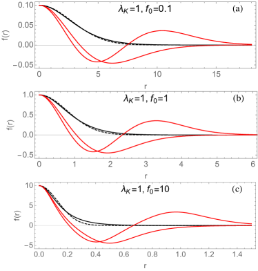
Figure 1: [Color online] The ground state solution for $\lambda_{K}=1$, $f_{0}=0.1,1,10$ compared to a gaussian (dashed line). In red, the solutions with one and two nodes in each case.

III.1.1 Ground state

In figure 2, we depict how the power and propagation constant vary within the family of ground state solutions with $\lambda_{K}=1$, that interpolate between the solution without Kerr term for $f_{0}\to 0$ and the one with only Kerr term, namely the Townes profile PhysRevLett.13.479 , for $f_{0}\to\infty$. Explicitly, for small $f_{0}$, we have $P\approx 2.40f_{0}$, $\mu\approx 10.53f_{0}+1.20f_{0}\log f_{0}$, where the logarithmic term is related to the boundary condition for $\phi(R)$. For the large $f_{0}$, we have $P\approx 5.85$ and $\mu\approx 0.205f_{0}^{2}+\left(26.9+5.85\log f_{0}\right)$. The $\mu$ is the sum of the one of the Townes solution plus a term coming from the value of $\phi(r)$ at small $r$. Notice that the light intensity is confined to a small region in $r<r_{sol}$ where $\phi$ reaches its minimum. Away from it, $\phi(R)\approx\phi(r_{sol})+P\log\frac{R}{r_{sol}}$. Thus, from our boundary condition $\phi(100)=0$, we find $\phi(r_{sol})=-P\log\frac{100}{r_{sol}}$, where $r_{sol}\approx f_{0}^{-1}$ for the Townes profile.

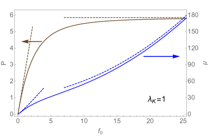
Figure 2: [Color online] The adimensional power $P$ and propagation constant $\mu$ as a function of $f_{0}$ for the Schrödinger-Poisson equation with focusing Kerr term $\lambda_{K}=1$. Dashed lines represent the asymptotic behaviors described in the text.

Both $P(f_{0})$ and $\mu(f_{0})$ are monotonically increasing functions. Thus $\frac{dP}{d\mu}$ is always positive within the family and all solutions are stable according to the Vakhitov-Kolokolov criterion. Clearly this derivative approaches zero for large $f_{0}$, as expected for the Townes profile.

III.1.2 Excited states and details on evolution algorithms

Let us now turn to excited states $i\geq 1$. In figure 3, we show an example of the disintegration of the solution with $f_{0}=3$ with two nodes. The computation of figure 3 and the rest of dynamical simulations displayed in this paper are performed setting boundary conditions in the sides of a square. The reason is that radial symmetry is not usually preserved by the actual pieces of thermo-optical material used in experiments segev ; PhysRevLett.95.213904 . In order to compare to the dark matter scenario, the best would be to fix the boundary conditions to match the monopolar contribution of the Poisson field sourced by the energy distribution. In a non-cylindrical sample material, this requires generating a space dependent particular temperature distribution at the boundary, which seems difficult to implement experimentally. Thus, we still fix constant $\Phi$ conditions at the borders of the square. We remark that radial symmetry is broken in a soft way if the square is much larger than the beam size and the main features of the evolution are not affected by this mismatch. Our simulations are performed using the beam propagation method to solve Eq. (1) and a finite difference scheme to solve Eq. (2) at each step. Convergence of the method has been checked by comparing simulations with different spacing for the spatial computational grids and steps in $z$.

We have not found any excited state stationary solution that preserves its shape for long propagation distances. Fig. 3 shows the initial stages of the disintegration of an unstable solution. Following the propagation to larger $z$, the system typically tends towards a ground state solution, surrounded by some radiation that takes the excess energy. This is similar to what we will discuss in section IV.c. The analogue behavior in three dimensions was analyzed in PRD69 . When the total power is above the Townes critical value $P\approx 5.85$, the evolution can eventually result in collapse, with $\psi$ diverging at finite $z$. When the beam profile becomes extremely narrow, the nonlocal term is negligible and the collapse is equivalent to that with only focusing Kerr term.

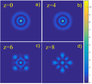
Figure 3: [Color online] An illustration of the initial stages of the evolution of an unstable solution with two nodes, $\lambda_{K}=1$ and $f_{0}=3$. The size of the images is 10 $\times$ 10 (dimensionless units). Boundary conditions $\phi=0$ are set in the sides of a 20 $\times$ 20 square.

III.1.3 Oscillations around the center of the material

The radially symmetric solutions we have discussed require that the center of the thermo-optical material coincides with the center of the soliton. In a first approximation, if the light beam is shifted from the center of the material, the beam profile remains unchanged but its center feels a refractive index gradient which induces an oscillation Alfassi:07 ; Alberucci:07 ; Alberucci:07a ; Shou:09 . One can think of this phenomenon as a self-force mediated by boundary conditions. It can be understood in terms in terms of Green’s function for two dimensional Laplace equation on the disk.

$$G(\rho,\theta)=\frac{P}{2}\log\frac{\hat{\rho}^{2}+\rho^{2}-2\hat{\rho}\rho\cos(\theta-\hat{\theta})}{R^{2}+\hat{\rho}^{2}\rho^{2}/R^{2}-2\hat{\rho}\rho\cos(\theta-\hat{\theta})}$$ (11)

This expression solves (2) for a point source of power $P$ placed at $(\hat{x},\hat{y})$, namely $|\psi|^{2}=P\delta(x-\hat{x})\delta(y-\hat{y})$ and satisfies the boundary condition $\phi(R)=0$. We have introduced $\rho^{2}=x^{2}+y^{2}\leq R^{2}$, $\hat{\rho}^{2}=\hat{x}^{2}+\hat{y}^{2}<R^{2}$, $\theta=\arctan(y/x)$, and $\hat{\theta}=\arctan(\hat{y}/\hat{x})$. The Green function (11) is computed by considering an image at a distance $R^{2}/\hat{\rho}$ from the center of the disk. We can think of the self-force mediated by boundary conditions as the force performed by the image on the source Shou:09 .

Without loss of generality, consider a soliton with center at $x=x_{s}$ with $y_{s}=0$. Taking the gradient of the potential generated by the image, keeping only the leading terms in $|x_{s}|/R<1$ and using Ehrenfest theorem we find the approximate expression:

$$\frac{d^{2}x_{s}}{dz^{2}}\approx-2P\frac{x_{s}}{R^{2}}-2P\frac{x_{s}^{3}}{R^{4}}$$ (12)

where $x_{s}$ is the position of the soliton at propagation distance $z$. Notice that this restoring force induced by boundary conditions becomes negligible for large $R$ and fixed $x_{s}$. This means that, if the electromagnetic wave is confined in a given region, the role of boundaries diminishes when the piece of optical material is taken wider.

From (12), it is immediate to infer a periodic motion with a period in the propagation distance $Z\approx\left(\frac{\sqrt{2}\pi R}{\sqrt{P}}-\frac{3\pi x_{i}^{2}}{4\sqrt{2P}R}\right)$ for a soliton initially at rest at $x=x_{i}$.

We have performed a series of simulations, with boundary conditions $\phi=0$ set at the boundary of a square of side $L$, by placing solitons of different powers initially displaced a distance $x_{i}$ from the center of the square. As expected from the discussion above, there is an oscillation induced by the boundary conditions. The period of the oscillation follows the same kind of dependence on $P$, $L$ and $x_{i}$ as the one found analytically for the disk. From our numerics, we infer that the period in $z$ of the oscillation is:

$$Z\approx\left(3.38\frac{L}{\sqrt{P}}-8.2\frac{x_{i}^{2}}{\sqrt{P}L}\right)$$ (13)

In figure 4 we depict an example of the oscillation found by numerically solving the evolution equations and a comparison of Eq. (13) with the computed value of $Z$ for several cases.

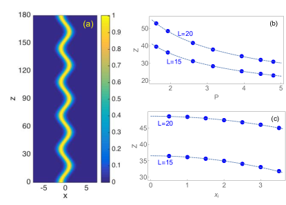
Figure 4: [Color online] Panel a) shows the oscillation in the $x$-direction for a particular example $f_{0}=1$ ($P\approx 1.93$), $x_{i}=-1$, $L=15$. We represent a contour plot $|\psi|^{2}(x,y=0,z)$. Panel b) represents examples of the numerically computed oscillation period with $x_{i}=-1$ for two values of $L$, compared to the model (13) (dashed line). Panel c) is a similar comparison as a function of $x_{i}$ with $P=1.93$ fixed.

III.2 b. Defocusing Kerr term

We now turn to the case of defocusing Kerr nonlinearity $\lambda_{K}=-1$. As in the previous case, for any $f_{0}>0$ there is a discrete set of values $\varphi_{0,i}(f_{0})$ which yield normalizable solutions with $i=0,1,2,\dots$ nodes for $f(r)$. Again, the ground state is always stable while we have not found stable excited solutions. Figure 5 shows several examples. Unsurprisingly, the solutions with $f_{0}=0.1$ are almost indistinguishable from those in figure 1, since the $f_{0}\to 0$ limit corresponds to negligible Kerr term. On the other hand, for large $f_{0}$, the difference becomes apparent. Curiously, in the intermediate case with $f_{0}=1$, the numerical solution is really similar to a gaussian.

Figure 5: [Color online] The ground state solution for $\lambda_{K}=-1$, $f_{0}=0.1,1,10$ compared to a gaussian (dashed line). In red, the solutions with one and two nodes in each case.

Figure 6 represents the power and propagation constant as a function of $f_{0}$ for the family of ground state solutions with $\lambda_{K}=-1$. For small $f_{0}$, we have $P\approx 2.40f_{0}$, $\mu\approx 10.53f_{0}+1.20f_{0}\log f_{0}$ as in the focusing case, since the Kerr term is unimportant in this limit. For large $f_{0}$, both nonlinearities play a decisive role. We have found by directly fitting the numerical data that both $P$ and $\mu$ grow quadratically $P\approx 1.27f_{0}^{2}$, $\mu\approx 5.88f_{0}^{2}$. A remarkable feature is that the size of the soliton solutions tends to a constant for large $f_{0}$. More precisely, the full width at half maximum of the distribution, defined as $f(r={\rm fwhm}/2)=f_{0}/\sqrt{2}$ asymptotes to $\lim_{f_{0}\to\infty}{\rm fwhm}\approx 1.21$, see the inset of figure 6.

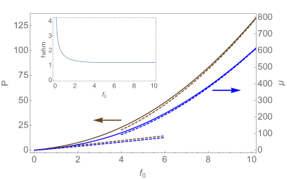
Figure 6: [Color online] The adimensional power $P$ and propagation constant $\mu$ as a function of $f_{0}$ for the Schrödinger-Poisson equation with defocusing Kerr term $\lambda_{K}=-1$. Dashed lines represent the asymptotic behaviors described in the text. In the inset, the full width at half maximum of the soliton solutions as a function of $f_{0}$.

Regarding oscillations mediated by boundary conditions, the dynamics with $\lambda_{K}=-1$ is rather similar to the one with focusing Kerr term because this effect is linked to the nonlocal nonlinearity while the local nonlinear term only affects the shape of the soliton itself but is hardly related to its overall motion.

IV IV. Soliton interactions and dark matter analogues

In this section, we provide several examples of the dynamics of interacting solitons by numerically analyzing Eqs. (1), (2). These simulations are relevant for the propagation of light in thermo-optical media, as described in section II. Moreover, they can be considered as analogues of galactic dark matter dynamics. In the context of the scalar field dark matter ($\psi$DM), soliton interactions have been studied in different situations, including head-on collisions guzman1 ; guzman2 ; Paredes:2015wga ; PhysRevD.93.103535 ; cotner , dipole-like structures PhysRevD.94.043513 and soliton mergers schiveprl ; PhysRevD.94.043513 . These works deal with Eqs. (1), (2) with one more transverse dimension $d=3$, but, as we will show, there are many qualitative similarities with the $d=2$ case. We remark that the dynamics of soliton collisions is of great importance in cosmology, since the wave-like evolution of $\psi$DM provides different outcomes from those of particle-like dark matter scenarios. Thus, it may furnish a way of improving our understanding of the nature and dynamics of dark matter, allowing us to discriminate between different scenarios and to make progress in one of the most important open problems of fundamental physics. For instance, wave interference at a galactic scale can induce large offsets between dark matter distributions and stars that might explain some recent puzzling observations Paredes:2015wga .

Some technical details of the numerical methods were briefly explained for Fig. 3 above. In order to generate initial conditions, we use the $f(r)$ profiles of the eigenstates discussed in section III:

$$\psi|_{z=0}=\sum_{i=1}^{n_{sol}}f_{i}(|{{\bf x}-{\bf x}_{i}|})e^{i({\bf v}_{i}\cdot{\bf x}+\phi_{i})}$$ (14)

where the sum runs over a number $n_{sol}$ of initial solitons with initial positions ${\bf x}_{i}$, phases $\phi_{i}$ and “velocities” ${\bf v}_{i}$. From now on, for $dx_{s}/dz$ we use the word velocity , which is appropriate for matter waves. In the optical setup, this quantity is of course the angle of propagation with respect to the axis. Boldface characters represent two-dimensional vectors ${\bf x}=(x,y)$, etc. In the examples displayed below, boundary conditions $\Phi=0$ are set at the perimeter of a square of side $L=20$ and center at ${\bf x}=0$.

IV.1 a. Head-on collisions

We start by analyzing the encounter of two solitons of the same power with equal phases. In the cosmological three-dimensional setup, this kind of problem has been addressed in guzman1 ; guzman2 ; Paredes:2015wga ; PhysRevD.93.103535 . Qualitative results are very similar in the present $d=2$ optical setup. What happens during evolution largely depends on the initial relative velocity as we describe below.

For large velocities, where for large we mean that ${|\bf v}|$ is larger than the inverse size of the initial structures, the solitons cross each other. During the collision, a typical interference fringe pattern is produced. Moreover, some tiny fraction of energy is radiated away from the solitons. We stress that we are using the word soliton in a loose sense, since the theory is not integrable and therefore even if the solitary waves cross each other, they do not come out undistorted. This behavior is depicted in figure 7. After the crossing, the non-local attraction and the self-interaction mediated by boundary conditions pull the solitons against each other again and, depending on the particular case, this might result in a second collision.

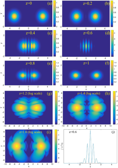
Figure 7: [Color online] Two solitons crossing each other and producing an interference pattern when they meet. The images (a)-(f) are contour plots of $|\psi|^{2}(x,y)$ at different values of the propagation distance $z$ for a numerical simulation of (1), (2) with $\lambda_{K}=1$. Panels (g)-(i) are contour plots of $\log_{10}(|\psi|^{2}(x,y))$ for the subsequent evolution. We use logarithmic scale in order to visualize the energy flowing away from the soliton centers (a meager $1\%$ in the example). Panel (h) depicts the interference pattern at $z=0.6$, integrated in $y$. Initial conditions are set by Eq. (14) with $n_{sol}=2$, $\phi_{i}=0$, $-x_{1}=x_{2}=3$, $v_{1}=-v_{2}=5$, $f_{0,1}=f_{0,2}=1.049$ ($P_{1}=P_{2}\approx 2$).

For intermediate velocities, solitons also cross each other but the associated wavelength is too small to generate a pattern with multiple fringes. Figure 8 shows an example.

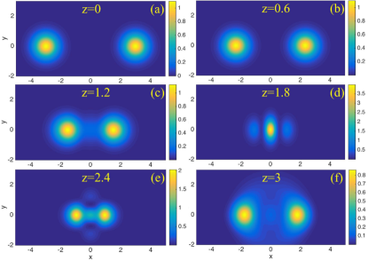
Figure 8: [Color online] Two solitons crossing each other with insufficient velocity to produce several interference fringes. All parameters are as in Fig. 7 except for $v_{1}=-v_{2}=1$.

For small velocities, the solitons merge in a fashion similar to subsection c below.

IV.2 b. Dipole-like configuration

As it is well known in different contexts, solitons in phase opposition repel each other. Possible consequences of this fact for galactic clusters were explored in Paredes:2015wga . In order to illustrate the fact, we consider a dipole-like structure: two solitons of the same size and power in phase opposition bounce back from each. Due to the nonlocal nonlinearity, they attract each other until they bounce back again and so on (see PhysRevD.94.043513 for similar consideration in the dark matter context). There is a competition between the attraction due to the Poisson term and the repulsion due to wave destructive interference. The Kerr term contributes to attraction or repulsion depending on its sign.

At this point, it is important to comment on the boundary conditions for the wave, since for large propagations part of the electromagnetic energy can reach the bound of the domain. We will consider absorbing conditions, which are the best suited for cosmological analogues. They can be implemented introducing at the borders a material with an imaginary part of the refractive index, but with the same real part as the one of the bulk. Mathematically, it can be modeled by introducing a “sponge”, as discussed for the three-dimensional dark matter case in guzman1 ; 0004-637X-645-2-814 ; PRD69 ; PRD74 . This amounts to adding a term:

$$-\frac{i}{4}V_{0}\left(4-\tanh\frac{x+\gamma}{\delta}+\tanh\frac{x-\gamma}{\delta}+\right.$$

$$\left.+\tanh\frac{y+\gamma}{\delta}+\tanh\frac{y-\gamma}{\delta}\right)\psi$$ (15)

to the right hand side of (1). This is a smooth version of a step function PRD69 . $\gamma$ fixes the position of the step and $\delta$ controls how steep the step is. In our simulations we fix $\gamma=0.4$, $\delta=0.2$, $V_{0}=1$.

Figure 9 shows an example of the bounces of a dipolar configuration, comparing the evolution for cases with $\lambda_{K}=\pm 1$ and the same soliton power. It is shown, that, eventually, the bouncing pattern becomes unstable and the solitons merge. As one could expect, this happens before for focusing Kerr nonlinearity $\lambda_{K}=+1$. Notice, however, that the values of $z$ reached in fig. 9 are much larger than those of the other figures of this section. This means that the instabilities only become manifest for long propagations. In fig 9, we also plot the $z$-evolution of the norm $N=\int|\psi|^{2}dxdy$, which decreases when the radiation approached the boundary because of the absorbing condition described above. This is the analogue of having scalar radiation flowing away from the region of interest in $\psi$DM. The figure shows that it starts happening when the instability breaks the initial solitons. The system eventually evolves into a pseudo-stationary state, similar to the one described in the next subsection.

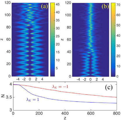
Figure 9: [Color online] Solitons in phase opposition bouncing against each other in a dipole-like structure and finally getting destabilized. We show contour plots of $|\psi|^{2}(x,z)$ integrated along $y$ for simulations of (1), (2) with $n_{sol}=2$, $v_{1}=v_{2}=0$, $\phi_{2}-\phi_{1}=\pi$. In panel (a), $\lambda_{K}=-1$ (defocusing Kerr term), $-x_{1}=x_{2}=3$, $f_{0,1}=f_{0,2}=0.7097$ ($P_{1}=P_{2}=2$). In panel (b), $\lambda_{K}=1$ (focusing Kerr term), $-x_{1}=x_{2}=2.6$, $f_{0,1}=f_{0,2}=1.409$ ($P_{1}=P_{2}=2$). Panel (c) portrays how the norm decreases due to the “sponge potential”, showing that when the dipolar structure breaks down and the soliton merge, a fraction of energy is radiated away.

We have not found any stable dipolar structure, but this aspect might deserve further research.

IV.3 c. Soliton mergers

In the $\psi$DM model of cosmology, the outcome of the merging of solitons has important consequences for the galactic dark matter distributions. In schiveprl ; PhysRevD.94.043513 , it was proven that the final configuration of such a process is a new, more massive, soliton (to be identified with a galactic core) surrounded by an incoherent distribution of matter with its density decreasing with a power law. The gravitational attraction prevents that this halo is radiated away. Here, we will show that a very similar behavior takes place in $d=2$, paving the way for optical experiments partially mimicking galactic mergers.

Figure 10 depicts an example of the initial stages of evolution of four equal merging solitons. The Kerr nonlinearity has been taken to be focusing and the total power to be below Townes’ threshold in order to avoid a possible collapse. The solitons rapidly coalesce and form a peaked narrow structure with a faint distribution of power around it.

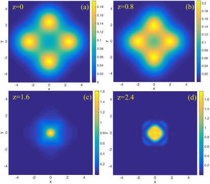
Figure 10: [Color online] Four merging solitons. The images are contour plots of $|\psi|^{2}(x,y)$ at different values of $z$ for a simulation with $\lambda_{K}=1$. Initial conditions are set by Eq. (14) with $n_{sol}=4$, $\phi_{i}=0$, $-x_{1}=x_{2}=-y_{3}=y_{4}=2.6$, $v_{i}=0$, $f_{0,i}=0.4$ (the power of the entire configuration is $P\approx 5.14$).

Continuing the numerical evolution of Eqs. (1), (2) to large values of $z$, a pseudo-stationary situation is attained, with an oscillation about a soliton profile at its center and incoherent radiation around it. This is shown in figure 11, where we depict an average in $z$ of the density profile depending on the distance to the center. We do the computation for the absorbing boundary condition presented in section IV.b. We also include an example with defocusing Kerr term $\lambda_{K}=-1$.

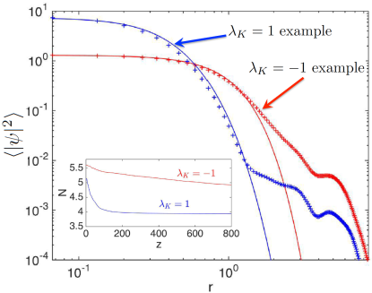
Figure 11: [Color online] Doubly logarithmic plot depicting the asymptotic power distribution for the simulation of figure 10 ($\lambda_{K}=1$) and another simulation with $\lambda_{K}=-1$ (four initial solitons with $f_{0}=4$, $\phi_{i}=0$, $-x_{1}=x_{2}=-y_{3}=y_{4}=3$, $P\approx 5.61$). The crosses are the result of the numerical computations and the solid lines represent the soliton profiles (section III) with the same energy density at $r=0$. In the vertical axis, $\langle|\psi|^{2}\rangle$ represents an average in $z$, taken over the interval $z\in[600,800]$ and along the line $y=0$, $x>0$, but the result depends only mildly in this particular choices. In the inset, we depict the $z$-evolution of the norm $N=\int|\psi|^{2}dxdy$ due the absorbing potential (15), showing that some energy is radiated away during the merging and then, slowly, the configuration tends to a pseudo-stationary situation.

The graphs show that, roughly speaking, the merging results in a soliton surrounded by a halo of energy trapped by “gravity”. Part of the initial energy has been radiated away during the merging of the solitonic structures. Their qualitative agreement with those of schiveprl ; PhysRevD.94.043513 is apparent. The force mediated by boundary conditions for $\Phi$ affects the result but does not change the qualitative picture with respect to the three-dimensional case.

V V. Conclusions

We have analyzed the Schrödinger-Poisson equations (1), (2) in two dimensions ($d=2$) in the presence of a Kerr term. We have limited the discussion to positive sign for the Poisson term. The model is relevant to describe laser propagation in thermo-optical materials, among other physical systems. With radially symmetric boundary conditions for $\Phi$, we have found uniparametric families of radially symmetric stable solitons. When the Kerr term is focusing, the family interpolates between the solution without Kerr term and the Townes profile. For defocusing Kerr term, the family interpolates between the solution without Kerr term and solitons which asymptotically tend to a particular finite size. The fixed boundary conditions induce effective forces which push the solitons towards the center of the material.

Regarding interactions, the Poisson term produces attraction at a distance, resembling gravity. This fact has been studied experimentally segev . Both the local and nonlocal nonlinearities shape the solitons and the results of dynamical evolution. However, we remark that in soliton collisions, a prominent role is played by the wave nature of Schrödinger equation. As in many nonlinear systems, interference fringes appear for appropriate initial conditions and there is attraction/repulsion for phase coincidence/opposition.

We have remarked that the same equations, in one more dimension ($d=3$), are the basis of the scalar field dark matter ($\psi$DM) model of cosmology, which relies on the hypothesis of the existence of a cosmic Bose-Einstein condensate of an ultralight axion. In this scenario, the physics of solitons is connected to phenomena taking place at length scales comparable to galaxies.

Certainly, there are differences between the cosmological $d=3$ case and the possible laboratory $d=2$ setups. First of all, we have not considered situations with evolution of the cosmic scale factor. Furthermore, the Poisson interaction is stronger in smaller dimension and the monopolar “gravitational force” decays as $1/r$ in $d=2$ rather than as $1/r^{2}$. It is of particular importance the role of boundary conditions. In the Universe, one typically has open boundary conditions. In a laboratory experiment, they have to be specified at a finite distance from the center. For the Poisson field (temperature), the simplest is to make it constant at the borders of the sample, even if this generates restoring forces towards the center. For the electromagnetic wave, the best is to introduce an absorbing element that prevents reflections towards the center of the radiation reaching the borders. This simulates the sponge typically used in the numerical $3d$ computations. In any case, the effects related to boundary conditions are reduced by taking larger two-dimensional sections of the optical material. We see no obstruction, apart from cost, to utilizing large pieces of glass in this kind of experiment. Let us also remark that, apart from the analogy discussed here, boundary conditions are a useful turning knob in optical experiments with nonlocal nonlinearities.

Despite these discrepancies and the disparate physical scales involved, there are apparent strong similarities between the families of self-trapped waves, their stability and their interactions in the $d=2$ and $d=3$ cases. We emphasize that this resemblance holds with or without Kerr term, corresponding to the presence or absence of non-negligible local self-interactions of the scalar in the cosmological setup. We hope that these considerations will pave the way for the experimental engineering of optical experiments that introduce analogues of dark matter dynamics in the $\psi$DM scenario.

VI Appendix: Scaling the equation to its canonical form

Consider the equation:

$$ia_{1}\frac{\partial\tilde{\psi}}{\partial\tilde{z}} = -\frac{1}{2}a_{2}\tilde{\nabla}^{2}\tilde{\psi}-\lambda_{K}a_{3}|\tilde{\psi}|^{2}\tilde{\psi}+a_{4}\tilde{\Phi}\tilde{\psi}$$ (16)

$$\tilde{\nabla}^{2}\tilde{\Phi} = a_{5}|\tilde{\psi}|^{2}$$ (17)

where the $a_{i}>0$ are constants and tilded quantities correspond to dimensionful coordinates, potential and wave function. Equations (16), (17) are transformed into the canonical dimensionless form (1), (2) by the following rescalings.

$$\tilde{z}=\frac{Ca_{1}a_{3}}{a_{2}a_{4}a_{5}}z,\qquad\quad\ (\tilde{x},\tilde{y})=\left(\frac{Ca_{3}}{a_{4}a_{5}}\right)^{\frac{1}{2}}(x,y)$$

$$\tilde{\psi}=\left(\frac{a_{2}a_{4}a_{5}}{Ca_{3}^{2}}\right)^{\frac{1}{2}}\psi,\qquad\ \tilde{\Phi}=\frac{a_{2}a_{5}}{Ca_{3}}\Phi.$$ (18)

- (1) Y. S. Kivshar and G. P. Agrawal, Optical Solitons. Academic Press, 2003.
- (2) B. A. Malomed, D. Mihalache, F. Wise, and L. Torner, “Spatiotemporal optical solitons,” J. Opt. B: Quantum Semiclass. Opt., 7, R53 (2005).
- (3) Z. Chen, M. Segev, and D. N. Christodoulides, “Optical spatial solitons: historical overview and recent advances,” Rep. Prog. Phys. 75, 086401 (2012).
- (4) R. Ruffini and S. Bonazzola, “Systems of self-gravitating particles in general relativity and the concept of an equation of state,” Phys. Rev. 187, 1767 (1969).
- (5) L. Diósi, “Gravitation and quantum-mechanical localization of macro-objects,” Phys. Lett. A 105, 199 (1984).
- (6) R. Penrose, “On gravity’s role in quantum state reduction,” Gen. Rel. Gravit. 28, 581 (1996).
- (7) R. Penrose, “On the gravitization of quantum mechanics 1: Quantum state reduction,” Found. Phys. 44, 557 (2014).
- (8) M. Bahrami, A. Grossardt, S. Donadi, and A. Bassi, “The Schrödinger-Newton equation and its foundations,” New J. Phys. 16, 115007 (2014).
- (9) D. O’Dell, S. Giovanazzi, G. Kurizki, and V. M. Akulin, “Bose-Einstein condensates with interatomic attraction: Electromagnetically induced “gravity”,” Phys. Rev. Lett. 84, 5687 (2000).
- (10) J. Qin, G. Dong, and B. A. Malomed, “Hybrid matter-wave microwave solitons produced by the local-field effect,” Phys. Rev. Lett. 115, 023901 (2015).
- (11) A. H. Guth, M. P. Hertzberg, and C. Prescod-Weinstein, “Do Dark Matter Axions Form a Condensate with Long-Range Correlation?,” Phys. Rev. D 92, 103513 (2015).
- (12) C. G. Böhmer and T. Harko, “Can dark matter be a Bose-Einstein condensate?,” J. Cosmol. and Astropart. Phys., 2007, 025 (2007).
- (13) A. Suárez, V. H. Robles, and T. Matos, “A review on the scalar field/Bose-Einstein condensate dark matter model,” in Accelerated Cosmic Expansion (C. Moreno González, J. E. Madriz Aguilar, and L. M. Reyes Barrera, eds.), vol. 38 of Astrophysics and Space Science Proceedings, pp. 107–142, Springer International Publishing, 2014.
- (14) D. J. Marsh, “Axion cosmology,” Phys. Rep. 643, 1 (2016).
- (15) H.-Y. Schive, T. Chiueh, and T. Broadhurst, “Cosmic structure as the quantum interference of a coherent dark wave,” Nat. Phys. 10, 496 (2014).
- (16) H.-Y. Schive, M.-H. Liao, T.-P. Woo, S.-K. Wong, T. Chiueh, T. Broadhurst, and W.-Y. P. Hwang, “Understanding the core-halo relation of quantum wave dark matter from 3d simulations,” Phys. Rev. Lett. 113, 261302 (2014).
- (17) L. Hui, J.P. Ostriker, S. Tremaine, and E. Witten, “On the hypothesis that cosmological dark matter is composed of ultra-light bosons”, arXiv:1610.08297 (2016).
- (18) C. Conti, M. Peccianti, and G. Assanto, “Route to nonlocality and observation of accessible solitons,” Phys. Rev. Lett. 91, 073901 (2003).
- (19) Y. Izdebskaya, W. Krolikowski, N. F. Smyth, and G. Assanto, “Vortex stabilization by means of spatial solitons in nonlocal media,” J. Opt. 18, 054006 (2016).
- (20) R. Bekenstein, R. Schley, M. Mutzafi, C. Rotschild, and M. Segev, “Optical simulations of gravitational effects in the Newton-Schrödinger system,” Nat. Phys. 11, 872 (2015).
- (21) V. M. Pérez-García, H. Michinel, and H. Herrero, “Bose-Einstein solitons in highly asymmetric traps,” Phys. Rev. A 57, 3837 (1998).
- (22) K. E. Strecker, G. B. Partridge, A. G. Truscott, and R. G. Hulet, “Formation and propagation of matter-wave soliton trains,” Nature 417, 150 (2002).
- (23) L. Khaykovich, F. Schreck, G. Ferrari, T. Bourdel, J. Cubizolles, L. D. Carr, Y. Castin, and C. Salomon, “Formation of a matter-wave bright soliton,” Science 296, 1290 (2002).
- (24) D. R. Solli, C. Ropers, P. Koonath, and B. Jalali, “Optical rogue waves,” Nature 450, 1054 (2007).
- (25) T. G. Philbin, C. Kuklewicz, S. Robertson, S. Hill, F. König, and U. Leonhardt, “Fiber-optical analog of the event horizon,” Science 319, 1367 (2008).
- (26) M. C. Braidotti, Z. H. Musslimani, and C. Conti, “Generalized uncertainty principle and analogue of quantum gravity in optics”, Physica D: Nonlinear Phenomena, in press, 2016.
- (27) J.W. Lee and I.G. Koh, “Galactic halos as boson stars,” Phys. Rev. D 53, 2236 (1996).
- (28) J. Goodman, “Repulsive dark matter,” New Astron. 5, 103 (2000).
- (29) A. Bernal and F. S. Guzmán, “Scalar field dark matter: Head-on interaction between two structures,” Phys. Rev. D 74, 103002 (2006).
- (30) C. Rotschild, O. Cohen, O. Manela, M. Segev, and T. Carmon, “Solitons in nonlinear media with an infinite range of nonlocality: First observation of coherent elliptic solitons and of vortex-ring solitons,” Phys. Rev. Lett. 95, 213904 (2005).
- (31) A. Alberucci, M. Peccianti, and G. Assanto, “Nonlinear bouncing of nonlocal spatial solitons at the boundaries,” Opt. Lett. 32, 2795 (2007).
- (32) A. Alberucci and G. Assanto, “Propagation of optical spatial solitons in finite-size media: interplay between nonlocality and boundary conditions,” J. Opt. Soc. Am. B 24, 2314 (2007).
- (33) B. Alfassi, C. Rotschild, O. Manela, M. Segev, and D. N. Christodoulides, “Boundary force effects exerted on solitons in highly nonlocal nonlinear media,” Opt. Lett. 32, 154 (2007).
- (34) I. B. Burgess, M. Peccianti, G. Assanto, and R. Morandotti, “Accessible light bullets via synergetic nonlinearities,” Phys. Rev. Lett. 102, 203903 (2009).
- (35) H. C. Gurgov and O. Cohen, “Spatiotemporal pulse-train solitons,” Opt. Express 17, 7052 (2009).
- (36) U. A. Laudyn, M. Kwasny, A. Piccardi, M. A. Karpierz, R. Dabrowski, O. Chojnowska, A. Alberucci, and G. Assanto, “Nonlinear competition in nematicon propagation,” Opt. Lett. 40, 5235 (2015).
- (37) K.-H. Kuo, Y.Y. Lin, R.-K. Lee, and B. A. Malomed, “Gap solitons under competing local and nonlocal nonlinearities,” Phys. Rev. A 83, 053838 (2011).
- (38) A. Paredes, D. Feijoo, and H. Michinel, “Coherent cavitation in the liquid of light,” Phys. Rev. Lett. 112, 173901 (2014).
- (39) F. Maucher, T. Pohl, S. Skupin, and W. Krolikowski, “Self-organization of light in optical media with competing nonlinearities,” Phys. Rev. Lett. 116, 163902 (2016).
- (40) Y.-C. Zhang, Z.-W. Zhou, B. A. Malomed, and H. Pu, “Stable solitons in three dimensional free space without the ground state: Self-trapped Bose-Einstein condensates with spin-orbit coupling,” Phys. Rev. Lett. 115, 253902 (2015).
- (41) D. Novoa, D. Tommasini, and H. Michinel, “Ultrasolitons: Multistability and subcritical power threshold from higher-order kerr terms,” EPL 98, 44003 (2012).
- (42) V. M. Pérez-García, V. V. Konotop, and J. J. García-Ripoll, “Dynamics of quasicollapse in nonlinear schrödinger systems with nonlocal interactions,” Phys. Rev. E 62, 4300 (2000).
- (43) O. Bang, W. Krolikowski, J. Wyller, and J. J. Rasmussen, “Collapse arrest and soliton stabilization in nonlocal nonlinear media,” Phys. Rev. E 66, 046619 (2002).
- (44) W. Kroikowski, O. Bang, N. I. Nikolov, D. Neshev, J. Wyller, J. J. Rasmussen, and D. Edmundson, “Modulational instability, solitons and beam propagation in spatially nonlocal nonlinear media,” J. Opt. B: Quantum Semiclass. Opt. 6, S288 (2004).
- (45) C. Rotschild, B. Alfassi, O. Cohen, and M. Segev, “Long-range interactions between optical solitons,” Nat. Phys. 2, 769 (2006).
- (46) Y. V. Kartashov, L. Torner, V. A. Vysloukh, and D. Mihalache, “Multipole vector solitons in nonlocal nonlinear media,” Opt. Lett. 31, 1483 (2006).
- (47) S. Lopez-Aguayo, A. S. Desyatnikov, Y. S. Kivshar, S. Skupin, W. Krolikowski, and O. Bang, “Stable rotating dipole solitons in nonlocal optical media,” Opt. Lett. 31, 1100 (2006).
- (48) I. M. Moroz, R. Penrose, and P. Tod, “Spherically-symmetric solutions of the Schrödinger-Newton equations,” Class. Quantum Grav. 15, 2733 (1998).
- (49) R. Harrison, I. Moroz, and K. P. Tod, “A numerical study of the Schrödinger- Newton equations,” Nonlinearity 16, 101 (2003).
- (50) I. Papadopoulos, P. Wagner, G. Wunner, and J. Main, “Bose-Einstein condensates with attractive interaction: The case of self-trapping,” Phys. Rev. A 76, 053604 (2007).
- (51) H. Cartarius, T. Fabcic, J. Main, and G. Wunner, “Dynamics and stability of Bose-Einstein condensates with attractive interaction,” Phys. Rev. A 78, 013615 (2008).
- (52) S. Rau, J. Main, H. Cartarius, P. Köberle, and G. Wunner, “Variational methods with coupled gaussian functions for Bose-Einstein condensates with long-range interactions. II. applications,” Phys. Rev. A 82, 023611 (2010).
- (53) F. S. Guzmán and L. A. Ureña-López, “Gravitational cooling of self-gravitating Bose condensates,” Astrophys. J. 645, 814 (2006).
- (54) P.-H. Chavanis and L. Delfini, “Mass-radius relation of newtonian self-gravitating Bose-Einstein condensates with short-range interactions. ii. numerical results,” Phys. Rev. D 84, 043532 (2011).
- (55) D. J. E. Marsh and A.-R. Pop, “Axion dark matter, solitons and the cusp-core problem,” Mon. Not. R. Astron. Soc. 451, 2479 (2015).
- (56) A. I. Yakimenko, Y. A. Zaliznyak, and Y. Kivshar, “Stable vortex solitons in nonlocal self-focusing nonlinear media,” Phys. Rev. E 71, 065603 (2005).
- (57) S. Ouyang and Q. Guo, “-dimensional strongly nonlocal solitons,” Phys. Rev. A 76, 053833 (2007).
- (58) A. Alberucci, C. P. Jisha, N. F. Smyth, and G. Assanto, “Spatial optical solitons in highly nonlocal media,” Phys. Rev. A 91, 013841 (2015).
- (59) A. Alberucci, C. P. Jisha, and G. Assanto, “Accessible solitons in diffusive media,” Opt. Lett. 39, 4317 (2014).
- (60) A. Alberucci, C. P. Jisha, and G. Assanto, “Breather solitons in highly nonlocal media,” arXiv:1602.01722 (2016).
- (61) V. Singh and P. Aghamkar, “Surface plasmon enhanced third-order optical nonlinearity of Ag nanocomposite film,” Appl. Phys. Lett. 104 (2014).
- (62) B. Can-Uc, R. Rangel-Rojo, A. P. na Ramírez, C. B. de Araújo, H. T. M. C. M. Baltar, A. Crespo-Sosa, M. L. Garcia-Betancourt, and A. Oliver, “Nonlinear optical response of platinum nanoparticles and platinum ions embedded in sapphire,” Opt. Express 24, 9955 (2016).
- (63) A. W. Snyder and D. J. Mitchell, “Accessible solitons,” Science 276, 1538 (1997).
- (64) R. Y. Chiao, E. Garmire, and C. H. Townes, “Self-trapping of optical beams,” Phys. Rev. Lett. 13, 479 (1964).
- (65) F. S. Guzmán, and L. A. Ureña-López, “Evolution of the Schrödinger-Newton system for a self-gravitating scalar field”, Phys. Rev. D 69, 0124033 (2004).
- (66) Q. Shou, Y. Liang, Q. Jiang, Y. Zheng, S. Lan, W. Hu, and Q. Guo, “Boundary force exerted on spatial solitons in cylindrical strongly nonlocal media,” Opt. Lett. 34, 3523 (2009).
- (67) J. A. González and F. S. Guzmán, “Interference pattern in the collision of structures in the Bose-Einstein condensate dark matter model: Comparison with fluids,” Phys. Rev. D 83, 103513 (2011).
- (68) A. Paredes and H. Michinel, “Interference of dark matter solitons and galactic offsets,” Phys. Dark Univ. 12, 50 (2016).
- (69) F. S. Guzmán, J. A. González, and J. P. Cruz-Pérez, “Behavior of luminous matter in the head-on encounter of two ultralight BEC dark matter halos,” Phys. Rev. D 93, 103535 (2016).
- (70) E. Cotner, “Collisional interactions between self-interacting non-relativistic boson stars: effective potential analysis and numerical simulations,” Phys. Rev. D 94, 063503 (2016).
- (71) B. Schwabe, J. C. Niemeyer, and J. F. Engels, “Simulations of solitonic core mergers in ultralight axion dark matter cosmologies,” Phys. Rev. D 94, 043513 (2016).
- (72) A. Bernal, and F. S. Guzmán, “Scalar field dark matter: Nonspherical collapse and late-time behavior”, Phys. Rev. D 74, 063504 (2006).