Jacobi-Davidson method on low-rank matrix manifolds

Abstract

In this work we generalize the Jacobi-Davidson method to the case when eigenvector can be reshaped into a low-rank matrix. In this setting the proposed method inherits advantages of the original Jacobi-Davidson method, has lower complexity and requires less storage. We also introduce low-rank version of the Rayleigh quotient iteration which naturally arises in the Jacobi-Davidson method.

1 Introduction

This paper considers generalization of the Jacobi-Davidson (JD) method [26] for finding target eigenvalue $\lambda$ (extreme or closest to a given number) and the corresponding eigenvector $x$ of $N\times N$ matrix $A$:

$$Ax=\lambda x.$$

We treat the specific case when $N=nm$ and the eigenvector $x$ reshaped into $n\times m$ matrix is exactly or approximately of small rank $r$. For example, consider a Laplacian operator discretized on tensor product grid; its reshaped eigenvectors are of rank $1$. For $r\ll n,m$ our assumption allows to significantly reduce storage of the final solution, at the same time leading to algorithmic complications that we address in this paper.

Similarly to the original JD method, we derive the low-rank Jacobi correction equation and propose low-rank version of subspace acceleration. The proposed approach takes the advantage of the original JD method. Compared with the Rayleigh quotient iteration and the Davidson approach, the method is efficient for the cases when arising linear systems are solved both accurately and inexactly.

The JD method is known to be a Riemannian Newton method on a unit sphere $\{x:\|x\|=1\}$ with additional subspace acceleration [1]. We utilize this interpretation and derive a new method as an inexact Riemannian Newton method on the intersection of the sphere and the fixed-rank manifold. In derivation we assume that the matrix $A$ is real and symmetric, however we test our approach on non-symmetric matrices as well. Complexity of the proposed algorithm scales as $\mathcal{O}\left((n+m)r(R+r)\right)$ if $A$ can be approximated as

$$A\approx\sum_{\alpha=1}^{R}F_{\alpha}\otimes G_{\alpha},$$

where $F_{\alpha}$ and $G_{\alpha}$ allow fast matrix-vector multiplication, e.g. they are sparse.

Our main contributions are:

• We generalize the Jacobi correction equation (Sec. 3) and the subspace acceleration (Sec. 4) to the case of fixed-rank matrix manifolds.

• We introduce low-rank version of the Rayleigh quotient iteration (Sec. 5) which naturally arises in the JD method.

2 Rayleigh quotient minimization on sphere

The first ingredient of the JD method is the Jacobi correction equation. The Jacobi correction equation can be derived as a Riemannian Newton method on the unit sphere [1], which will be useful for our purposes. In this section we provide the derivation, and in Sec. 3 it will be generalized to the low-rank case.

Given a symmetric matrix $A\in\mathbb{R}^{n\times n}$ the goal is to optimize

$$\mathfrak{R}(x)=x^{\top}Ax,$$ (1)

subject to $x\in S^{n-1}$, where $S^{n-1}$ is a unit sphere considered as an embedded submanifold of $\mathbb{R}^{n}$ with the pullback metric $g_{x}(\xi,\eta)=\xi^{\top}\eta$. The Riemannian optimization approach implies that we optimize $\mathfrak{R}(x)$ on $S^{n-1}$, i.e. constraints are already accounted for in the search space. One of the key concepts in the Riemannian optimization is a tangent space which is in fact a linearization of the manifold at a given point. The orthogonal projection of $\xi$ on the tangent space $T_{x}S^{n-1}$ of $S^{n-1}$ at $x$ can be written as [1]

$$\mathrm{P}_{T_{x}S^{n-1}}\xi=(I-xx^{\top})\xi.$$ (2)

The Riemannian gradient of (1) is

$$\mathop{\operator@font grad}\nolimits\mathfrak{R}(x)=\mathrm{P}_{T_{x}S^{n-1}}\nabla\mathfrak{R}(x)=(I-xx^{\top})(2Ax),$$ (3)

where $\nabla$ denotes the Euclidean gradient. The Hessian $\mathrm{Hess}_{x}:T_{x}S^{n-1}\to T_{x}S^{n-1}$ can be obtained as [2]

$$\begin{split}\mathrm{Hess}_{x}\,\mathfrak{R}(x)[\xi]=&\mathrm{P}_{T_{x}S^{n-1}}\left(\mathrm{D}\,\left(\mathrm{grad}\,\mathfrak{R}(x)\right)[\xi]\right)=\\ &2\mathrm{P}_{T_{x}S^{n-1}}\left(\mathrm{D}\left(\mathrm{P}_{T_{x}S^{n-1}}Ax\right)[\xi]\right)=\\ &2\mathrm{P}_{T_{x}S^{n-1}}(A\xi+\dot{\mathrm{P}}_{T_{x}S^{n-1}}Ax),\quad\xi\in T_{x}S^{n-1},\end{split}$$ (4)

where $\mathrm{D}$ denotes the differential map (directional derivative) and

$$\dot{\mathrm{P}}_{T_{x}S^{n-1}}Ax\equiv\mathrm{D}(\mathrm{P}_{T_{x}S^{n-1}})[\xi]Ax=-(x^{\top}Ax)\xi-(\xi^{\top}Ax)x.$$

Since $\mathrm{P}_{T_{x}S^{n-1}}x=0$ and $\mathrm{P}_{T_{x}S^{n-1}}\xi=\xi$ we arrive at

$$\mathrm{Hess}_{x}\,\mathfrak{R}(x)[\xi]=2\mathrm{P}_{T_{x}S^{n-1}}\left(A-(x^{\top}Ax)I\right)\mathrm{P}_{T_{x}S^{n-1}}\xi.$$ (5)

The $k$-th step of the Riemannian Newton methods looks as

$$\mathrm{Hess}_{x_{k}}\,\mathfrak{R}(x_{k})[\xi_{k}]=-\mathop{\operator@font grad}\nolimits\mathfrak{R}(x_{k}),\quad\xi_{k}\in T_{x_{k}}S^{n-1},$$ (6)

with the retraction

$$x_{k+1}=\frac{x_{k}+\xi_{k}}{\|x_{k}+\xi_{k}\|},$$ (7)

which returns $x_{k}+\xi_{k}$ back to the manifold $S^{n-1}$. Using (2), (3) and (5) we can rewrite (6) as

$$(I-x_{k}x_{k}^{\top})\left(A-\mathfrak{R}(x_{k})I\right)(I-x_{k}x_{k}^{\top})\xi_{k}=-r_{k},\quad x_{k}^{\top}\xi_{k}=0,$$ (8)

where

$$\mathfrak{R}(x_{k})=x_{k}^{\top}Ax_{k},\quad r_{k}=(I-x_{k}x_{k}^{\top})Ax_{k}=Ax_{k}-\mathfrak{R}(x_{k})x_{k}.$$

Equation (8) is called the Jacobi correction equation [26]. Note that without the projection $(I-x_{k}x_{k}^{\top})$ we obtain the Davidson equation

$$\left(A-\mathfrak{R}(x_{k})I\right)\xi_{k}=-r_{k},$$

which has solution $\xi_{k}=-x_{k}$ collinear to the current approximation $x_{k}$. This is the reason for the Davidson equation to be solved inexactly. The original Davidson algorithm [6] replaces $A$ by its diagonal part $\mathrm{diag}(A)$. By contrast, even if the Jacobi correction equation (8) is solved inexactly using Krylov iterative methods, its solution $\xi_{k}$ will be automatically orthogonal to $x_{k}$ which is beneficial for the computational stability. Moreover, since the JD method has the Newton interpretation it boasts local superlinear convergence.

The goal of this paper is to extend the Jacobi correction equation (8) and the second ingredient of the JD method — subspace acceleration — to the case of low-rank manifolds.

3 Jacobi correction equation on fixed-rank manifolds

Let $x\in\mathbb{R}^{nm}$ be an eigenvector of $A$ and $X\in\mathbb{R}^{n\times m}$ be its matricization: $x=\operatorname{vec}(X)$, where $\operatorname{vec}$ denotes columnwise reshape of $n\times m$ matrix into $nm$ vector. In this paper we make an assumption that matricisized eigenvector $X$ is approximately of rank $r$. Therefore, for example, to approximate the smallest eigenvalue we solve the following optimization problem

$$\begin{split}\text{minimize}\quad&\mathfrak{R}(x)=x^{\top}Ax\\ \text{s.t. }\quad&x\in S^{nm-1}\cap\mathcal{M}_{r},\end{split}$$ (9)

where

$$\mathcal{M}_{r}=\{\mathrm{vec}(X),\,X\in\mathbb{R}^{n\times m}:\text{rank}(X)=r\},$$

which forms a smooth embedded submanifold of $\mathbb{R}^{nm}$ of dimension $(m+n)r-r^{2}$ [19]. By analogy with the derivation of the Jacobi equation we additionally intersected the manifold $\mathcal{M}_{r}$ with the sphere $S^{nm-1}$. As we will see from the following proposition $S^{nm-1}\cap\mathcal{M}_{r}$ forms a smooth embedded submanifold of $\mathbb{R}^{nm}$. Hence, optimization problem (9) can be solved using Riemannian optimization techniques.

Proposition 1.

Let $\mathcal{N}=S^{nm-1}\cap\mathcal{M}_{r}$, then

1. $\mathcal{N}$ forms smooth embedded submanifold of $\mathbb{R}^{nm}$ of dimension $(n+m)r-r^{2}-1$

2. The tangent space of $\mathcal{N}$ at $\operatorname{vec}(X)\in\mathcal{N}$ with $X$ given by SVD: $X=USV^{\top}$, $U^{\top}U=I$, $V^{\top}V=I$, $S=\mathrm{diag}(\sigma_{1},\dots,\sigma_{r})$, $\sigma_{1}\geq\dots\geq\sigma_{r}>0$ can be parametrized as

   $$\begin{split}T_{X}\mathcal{N}=\{\operatorname{vec}(U_{\xi}V^{\top}+UV^{\top}_{\xi}+US_{\xi}V^{\top}):U_{\xi}\perp U,\,V_{\xi}\perp V,\,\operatorname{vec}(S_{\xi})\perp\operatorname{vec}(S)\}.\end{split}$$

3. The orthogonal projection $\mathrm{P}_{T_{X}\mathcal{N}}$ onto $T_{X}\mathcal{N}$ can be written as

   $$\mathrm{P}_{T_{X}\mathcal{N}} =\mathrm{P}_{T_{X}\mathcal{M}_{r}}\mathrm{P}_{T_{X}S^{nm-1}}=\mathrm{P}_{T_{X}S^{nm-1}}\mathrm{P}_{T_{X}\mathcal{M}_{r}}$$ (10)

   $$=\mathrm{P}_{T_{X}\mathcal{M}_{r}}-\mathrm{vec}(X)\mathrm{vec}^{\top}(X),$$

   where $\mathrm{P}_{T_{X}\mathcal{M}_{r}}$ is the orthogonal projection onto the tangent space of $\mathcal{M}_{r}$:

   $$\mathrm{P}_{T_{X}\mathcal{M}_{r}}=VV^{\top}\otimes UU^{\top}+VV^{\top}\otimes(I_{n}-UU^{\top})+(I_{m}-VV^{\top})\otimes UU^{\top}.$$

The first property follows from the fact that $\mathcal{M}_{r}$ and $S^{nm-1}$ are transversal embedded submanifolds of $\mathbb{R}^{nm}$. Indeed, one can easily verify that

$$T_{X}\mathcal{M}_{r}+T_{X}S^{nm-1}=\mathbb{R}^{nm}.$$

Hence, by the transversality property [19] $\mathcal{N}$ forms a smooth embedded submanifold of $\mathbb{R}^{nm}$ of dimension

$$\dim(\mathcal{M}_{r})+\dim(S^{nm-1})-\dim(\mathbb{R}^{nm})=(n+m-r)r-1$$

Let us prove the second property of the proposition. Vector $\xi\in T_{X}\mathcal{M}_{r}$ can be parametrized [27] as

$$\xi=\operatorname{vec}(U_{\xi}V^{\top}+UV^{\top}_{\xi}+US_{\xi}V^{\top})$$ (11)

with the gauge conditions

$$U_{\xi}\perp U,\quad V_{\xi}\perp V.$$ (12)

To obtain the parametrization of $\xi\in T_{X}S^{nm-1}\cap T_{X}\mathcal{M}_{r}$ we need to take into account that $\xi\in T_{X}S^{nm-1}$ and, hence, $\xi^{\top}x=0$ yielding the additional gauge condition

$$\text{vec}(S_{\xi})\perp\text{vec}(S).$$ (13)

Let us prove the third property by showing that operators $\mathrm{P}_{T_{X}\mathcal{M}_{r}}$ and $\mathrm{P}_{T_{X}S^{nm-1}}$ commute and, hence,

$$\mathrm{P}_{T_{X}\mathcal{N}}=\mathrm{P}_{T_{X}\mathcal{M}_{r}}\mathrm{P}_{T_{X}S^{nm-1}}=\mathrm{P}_{T_{X}S^{nm-1}}\mathrm{P}_{T_{X}\mathcal{M}_{r}}$$ (14)

is an orthogonal projection on the intersection of $T_{X}\mathcal{M}_{r}$ and $T_{X}S^{nm-1}$. Indeed, since

$$\operatorname{vec}(X)\operatorname{vec}\left(X\right)^{\top}=(V\otimes U)\operatorname{vec}(S)\left(\operatorname{vec}(S)\right)^{\top}(V^{\top}\otimes U^{\top}),$$

and

$$UU^{\top}(I-UU^{\top})=0,\quad VV^{\top}(I-VV^{\top})=0,$$

we get

$$\mathrm{P}_{T_{X}\mathcal{M}_{r}}\operatorname{vec}(X)\left(\operatorname{vec}(X)\right)^{\top}=\operatorname{vec}(X)\left(\operatorname{vec}(X)\right)^{\top}=\operatorname{vec}(X)\left(\operatorname{vec}(X)\right)^{\top}\mathrm{P}_{T_{X}\mathcal{M}_{r}}.$$

Finally, since $\mathrm{P}_{T_{X}S^{nm-1}}=I-\operatorname{vec}(X)\left(\operatorname{vec}(X)\right)^{\top}$

$$\begin{split}\mathrm{P}_{T_{X}\mathcal{N}}\mathrm{P}_{T_{X}\mathcal{N}}=&\ \mathrm{P}_{T_{X}\mathcal{M}_{r}}\mathrm{P}_{T_{X}S^{nm-1}}=\ \mathrm{P}_{T_{X}\mathcal{M}_{r}}(I-\operatorname{vec}(X)\left(\operatorname{vec}(X)\right)^{\top})\\ =&\ \mathrm{P}_{T_{X}\mathcal{M}_{r}}-\operatorname{vec}(X)\left(\operatorname{vec}(X)\right)^{\top}=\ \mathrm{P}_{T_{X}S^{nm-1}}\mathrm{P}_{T_{X}\mathcal{M}_{r}},\end{split}$$

which completes the proof.

3.1 Derivation of Jacobi correction equation on $\mathcal{N}$

Let us derive the generalization of the original Jacobi correction equation, which is the Riemannian Newton method on $\mathcal{N}$. Using (10) and notation $x=\operatorname{vec}(X)$ we obtain

$$\mathop{\operator@font grad}\nolimits\mathfrak{R}(x)=\mathrm{P}_{T_{X}\mathcal{N}}\nabla\mathfrak{R}(x)=\mathrm{P}_{T_{X}\mathcal{M}_{r}}(I-xx^{\top})\nabla\mathfrak{R}(x)=2\mathrm{P}_{T_{X}\mathcal{M}_{r}}(I-xx^{\top})Ax.$$ (15)

Similarly to (4) using (10) we get

$$\begin{split}\mathrm{Hess}_{X}\,\mathfrak{R}(x)[\xi]=&2\mathrm{P}_{T_{X}\mathcal{N}}(A\xi+\dot{\mathrm{P}}_{T_{X}\mathcal{N}}Ax)=\\ &2\mathrm{P}_{T_{X}\mathcal{N}}(A\xi-x\,\xi^{\top}Ax-\xi x^{\top}Ax+\dot{\mathrm{P}}_{T_{X}\mathcal{M}_{r}}Ax),\\ &\xi\in T_{X}\mathcal{N}.\end{split}$$

According to (10) $\mathrm{P}_{T_{X}\mathcal{N}}x=\mathrm{P}_{T_{X}\mathcal{M}_{r}}\mathrm{P}_{T_{X}S^{nm-1}}x=0$, thus

$$\begin{split}\mathrm{Hess}_{X}\,\mathfrak{R}(x)[\xi]=\ &2\mathrm{P}_{T_{X}\mathcal{N}}(A-(x^{\top}Ax)I)\xi+\mathrm{P}_{T_{X}\mathcal{N}}\dot{\mathrm{P}}_{T_{X}\mathcal{M}_{r}}Ax=\\ &2\mathrm{P}_{T_{X}\mathcal{M}_{r}}(I-xx^{\top})(A-(x^{\top}Ax)I)\xi+\mathrm{P}_{T_{X}\mathcal{N}}\dot{\mathrm{P}}_{T_{X}\mathcal{M}_{r}}Ax,\end{split}$$

where the part $\mathrm{P}_{T_{X}\mathcal{N}}\dot{\mathrm{P}}_{T_{X}\mathcal{M}_{r}}Ax$ corresponds to the curvature of the low-rank manifold. This term contains inverses of singular values. Singular values can be small if the rank is overestimated. This, therefore, leads to difficulties in numerical implementation. Similarly to [16] we omit this part and obtain an inexact Newton method, which can be viewed as a constrained Gauss-Newton method. Omitting $\mathrm{P}_{T_{X}\mathcal{N}}\dot{\mathrm{P}}_{T_{X}\mathcal{M}_{r}}Ax$ we get

$$\mathrm{Hess}_{X}\,\mathfrak{R}(x)[\xi]\approx 2\mathrm{P}_{T_{X}\mathcal{M}_{r}}(I-xx^{\top})(A-\mathfrak{R}(x)I)\xi,$$

or in the symmetric form

$$\mathrm{Hess}_{X}\,\mathfrak{R}(x)[\xi]\approx 2\mathrm{P}_{T_{X}\mathcal{M}_{r}}(I-xx^{\top})(A-\mathfrak{R}(x)I)(I-xx^{\top})\mathrm{P}_{T_{X}\mathcal{M}_{r}}\xi.$$ (16)

Using (15) and (16) we can write the linear system arising in the inexact Newton method as

$$\begin{split}(I-xx^{\top})\left[\mathrm{P}_{T_{X}\mathcal{M}_{r}}(A-\mathfrak{R}(x)I)\mathrm{P}_{T_{X}\mathcal{M}_{r}}\right]&(I-xx^{\top})\xi=-\mathrm{P}_{T_{X}\mathcal{M}_{r}}(I-xx^{\top})Ax,\\ \xi^{\top}x=0,&\quad\xi\in{T_{X}\mathcal{M}_{r}}.\end{split}$$ (17)

which has the form similar to the original Jacobi correction equation (8) with $(A-\mathfrak{R}(x)I)$ projected on $T_{X}\mathcal{M}_{r}$.

Equation (17) is a linear system of size $nm\times nm$, but the number of unknown elements is equal to dimension of the tangent space $(n+m)r-r^{2}-1$. Hence, the next step is to derive a local linear system that is of smaller size and is useful for the numerical implementation. The following proposition holds.

Proposition 2.

The solution of (17) written as

$$\xi=\operatorname{vec}(U_{\xi}V^{\top}+UV^{\top}_{\xi}+US_{\xi}V^{\top}),$$

can be found from the local system

$$(I-BB^{\top})(A-\mathfrak{R}(x)I)_{\mathrm{loc}}(I-BB^{\top})\tau_{\xi}=-(I-BB^{\top})g,\quad B^{\top}\tau_{\xi}=0,$$ (18)

where

$$\tau_{\xi}=\begin{bmatrix}\operatorname{vec}(U_{\xi})\\ \operatorname{vec}(V^{\top}_{\xi})\\ \operatorname{vec}(S_{\xi})\end{bmatrix},\quad g=\begin{bmatrix}A_{v,v}\,\operatorname{vec}(US)\\ A_{u,u}\,\operatorname{vec}(SV^{\top})\\ A_{vu,vu}\,\operatorname{vec}(S)\end{bmatrix},\quad B=\begin{bmatrix}I_{r}\otimes U&0&0\\ 0&V\otimes I_{r}&0\\ 0&0&\operatorname{vec}(S)\\ \end{bmatrix},$$

$$(A-\mathfrak{R}(x)I)_{\mathrm{loc}}=\begin{bmatrix}(A-\mathfrak{R}(x)I)_{v,v}&(A-\mathfrak{R}(x)I)_{v,u}&(A-\mathfrak{R}(x)I)_{v,uv}\\ (A-\mathfrak{R}(x)I)_{u,v}&(A-\mathfrak{R}(x)I)_{u,u}&(A-\mathfrak{R}(x)I)_{u,vu}\\ (A-\mathfrak{R}(x)I)_{vu,v}&(A-\mathfrak{R}(x)I)_{vu,u}&(A-\mathfrak{R}(x)I)_{vu,vu}\end{bmatrix},$$

Notice that $\mathrm{P}_{T_{X}\mathcal{M}_{r}}$ is a sum of three orthogonal projections

$$\begin{split}\mathrm{P}_{T_{X}\mathcal{M}_{r}}&=\mathrm{P}_{1}+\mathrm{P}_{2}+\mathrm{P}_{3},\\ \mathrm{P}_{1}=VV^{\top}\otimes(I_{n}-UU^{\top}),\quad\mathrm{P}_{2}&=(I_{m}-VV^{\top})\otimes UU^{\top},\quad\mathrm{P}_{3}=VV^{\top}\otimes UU^{\top}\end{split}$$

Since $\mathrm{P}_{i}\mathrm{P}_{j}=\mathrm{O}$, $i\not=j$ and $\mathrm{P}_{i}^{2}=\mathrm{P}_{i}$ we obtain

$$\begin{bmatrix}\mathrm{P}_{1}\\ \mathrm{P}_{2}\\ \mathrm{P}_{3}\end{bmatrix}(I-xx^{\top})(A-\mathfrak{R}(x)I)(I-xx^{\top})\begin{bmatrix}\mathrm{P}_{1}&\mathrm{P}_{2}&\mathrm{P}_{3}\end{bmatrix}\begin{bmatrix}\mathrm{P}_{1}\xi\\ \mathrm{P}_{2}\xi\\ \mathrm{P}_{3}\xi\end{bmatrix}=\begin{bmatrix}\mathrm{P}_{1}\\ \mathrm{P}_{2}\\ \mathrm{P}_{3}\end{bmatrix}(I-xx^{\top})Ax.$$ (19)

It is easy to verify that

$$\begin{split}\mathrm{P}_{1}(I-xx^{\top})=&\ \mathrm{P}_{1}=(V\otimes I_{n})(V^{\top}\otimes(I_{n}-UU^{\top})),\\ \mathrm{P}_{2}(I-xx^{\top})=&\ \mathrm{P}_{2}=(I_{m}\otimes U)((I_{m}-VV^{\top})\otimes U^{\top}),\\ \mathrm{P}_{3}(I-xx^{\top})=&\ (VV^{\top}\otimes UU^{\top})(I-(V\otimes U)\operatorname{vec}(S)\left(\operatorname{vec}(S)\right)^{\top}(V^{\top}\otimes U^{\top}))=\\ &(V\otimes U)(I_{r^{2}}-\operatorname{vec}(S)\left(\operatorname{vec}(S)\right)^{\top})(V^{\top}\otimes U^{\top}).\end{split}$$

Then from (11)

$$\begin{split}&\mathrm{P}_{1}\xi=V\otimes(I_{n}-UU^{\top})\,\operatorname{vec}(U_{\xi}),\\ &\mathrm{P}_{2}\xi=(I_{m}-VV^{\top})\otimes U\,\operatorname{vec}(V_{\xi}^{\top}),\\ &\mathrm{P}_{3}\xi=V\otimes U\,\operatorname{vec}(S_{\xi}),\\ \end{split}$$

Thus, the first block row in (19) can be written as

$$\begin{split}V\otimes(I_{n}-UU^{\top})(&\underbrace{(V^{\top}\otimes I)(A-\mathfrak{R}(x)I)(V\otimes I_{n})}_{(A-\mathfrak{R}(x)I)_{v,v}}(I_{r}\otimes(I_{n}-UU^{\top}))\operatorname{vec}(U_{\xi})+\\ &\underbrace{(V^{\top}\otimes I)(A-\mathfrak{R}(x)I)(I_{m}\otimes U)}_{(A-\mathfrak{R}(x)I)_{v,u}}((I_{m}-VV^{\top})\otimes I_{r})\operatorname{vec}(V^{\top}_{\xi})+\\ &\underbrace{(V^{\top}\otimes I)(A-\mathfrak{R}(x)I)(V\otimes U))}_{(A-\mathfrak{R}(x)I)_{v,uv}}(I_{r^{2}}-\operatorname{vec}(S)\left(\operatorname{vec}(S)\right)^{\top})\operatorname{vec}(S_{\xi})=\\ V\otimes(I_{n}-UU^{\top})&\underbrace{(V^{\top}\otimes I)A(V\otimes I_{n})}_{A_{v,v}}\operatorname{vec}(US).\end{split}$$

Since $V$ has full column rank we obtain exactly the first block row in (18). Other block rows can be obtained in a similar way.

3.2 Retraction

Similarly to (7) after we obtained the solution $\xi$ from (18) we need to map the vector $x+\xi$ from the tangent space back to the manifold. The following proposition gives an explicit representation for the retraction on $\mathcal{N}$.

Proposition 3.

Let $R_{r}$ be a retraction from the tangent bundle $T\mathcal{M}_{r}$ onto $\mathcal{M}_{r}$, then

$$R(X,\dot{X})=\frac{R_{r}(X,\dot{X})}{\|R_{r}(X,\dot{X})\|},$$ (20)

is a retraction onto $\mathcal{N}$.

To verify that $R$ is a retraction we need to check the following properties [3]

1. Smoothness on a neighborhood of the zero element in $T\mathcal{N}$;

2. $R(X,0)=X$ for all $X\in\mathcal{N}$;

3. $\left.\frac{d}{dt}R(X,t\dot{X})\right|_{t=0}=\dot{X}$ for all $X\in\mathcal{N}$ and $\dot{X}\in T_{X}\mathcal{N}$.

The first property follows from the smoothness of $R_{r}$. The second property holds since $R_{r}(X,0)=X$ and $\|X\|=1$ for $X\in\mathcal{N}$. Let us verify the third property:

$$\begin{split}&\left.\frac{d}{dt}R(X,t\dot{X})\right|_{t=0}=\left.\frac{d}{dt}\left(\frac{R_{r}(X,t\dot{X})}{\|R_{r}(X,t\dot{X})\|}\right)\right|_{t=0}=\\ &\frac{\left.\frac{d}{dt}R_{r}(X,t\dot{X})\right|_{t=0}\left.\|R_{r}(X,t\dot{X})\right|_{t=0}\|-\frac{d}{dt}\left.\|R_{r}(X,t\dot{X})\|\right|_{t=0}\left.R_{r}(X,t\dot{X})\right|_{t=0}}{\|\left.R_{r}(X,t\dot{X})\right|_{t=0}\|^{2}}.\end{split}$$ (21)

Since $(X,\dot{X})=0$ for $X\in\mathcal{N}$, we get

$$\begin{split}\left.\frac{d}{dt}\|R_{r}(X,t\dot{X})\|\right|_{t=0}&=\\ &\frac{\left.\left(\frac{d}{dt}R_{r}(X,t\dot{X}),R_{r}(X,t\dot{X})\right)\right|_{t=0}+\left.\left(R_{r}(X,t\dot{X}),\frac{d}{dt}R_{r}(X,t\dot{X})\right)\right|_{t=0}}{2\left.\|R_{r}(X,t\dot{X})\right|_{t=0}\|}\\ &=\frac{(\dot{X},X)+({X},\dot{X})}{2\|X\|}=0,\quad X\in\mathcal{N},\quad\dot{X}\in T_{X}\mathcal{N}.\end{split}$$

Substituting the latter expression into (21) and accounting for

$$\left.\|R_{r}(X,t\dot{X})\right|_{t=0}\|=\|R_{r}(X,0)\|=\|X\|=1$$

we obtain $\left.\frac{d}{dt}R(X,t\dot{X})\right|_{t=0}=\dot{X}$ which completes the proof.

Remark 1.

Retraction (20) is a composition of two retractions: first on the low-rank manifold $\mathcal{M}_{r}$ and then on the sphere $S^{n-1}$. Note that the composition in the reversed order is not a retraction as it does not map to the manifold $\mathcal{N}$.

A standard choice of retraction on $\mathcal{M}_{r}$ is [3]

$$R_{r}(x,\xi)\equiv R_{r}(x+\xi)=\mathrm{P}_{\mathcal{M}_{r}}(x+\xi),$$

where

$$\mathrm{P}_{\mathcal{M}_{r}}(x+\xi)\equiv\operatorname*{arg\,min}_{y\in\mathcal{M}_{r}}\|y-(x+\xi)\|.$$

For small enough correction $\xi$ retraction can be calculated using the SVD procedure [3] as follows. First,

$$\begin{split}x+\xi=\text{vec}(USV^{\top}+U_{\xi}V^{\top}+UV^{\top}_{\xi}+US_{\xi}V^{\top})=\\ \operatorname{vec}\left(\begin{bmatrix}U&U_{\xi}\end{bmatrix}\begin{bmatrix}S+S_{\xi}&I\\ I&O\end{bmatrix}\begin{bmatrix}V&V_{\xi}\end{bmatrix}^{\top}\right)\end{split}.$$

Then we calculate $QR$ decompositions

$$Q_{U}R_{U}=\begin{bmatrix}U&U_{\xi}\end{bmatrix},\quad Q_{V}R_{V}=\begin{bmatrix}V&V_{\xi}\end{bmatrix}.$$

and the truncated SVD with truncation rank $r$ of

$$R_{U}\begin{bmatrix}S+S_{\xi}&I\\ I&O\end{bmatrix}R_{V}^{\top},$$

with $r$ leading singular vectors $U_{r}\in\mathbb{R}^{2r\times r}$, $V_{r}\in\mathbb{R}^{2r\times r}$ and the matrix of leading $r$ singular values $S_{r}\in\mathbb{R}^{r\times r}$. Thus, the resulting retraction can be written as

$$R_{r}(x+\xi)=(Q_{U}U_{r})S_{r}(Q_{V}V_{r})^{\top}.$$

and from (20) the retraction has the form

$$R(x,\xi)\equiv R(x+\xi)=(Q_{U}U_{r})\frac{S_{r}}{\|S_{r}\|}(Q_{V}V_{r})^{\top}.$$ (22)

3.3 Properties of the local system

Let us mention several important properties of the matrix $(A-\mathfrak{R}(x)I)_{\text{loc}}$. Assume that we are looking for the smallest eigenvalue $\lambda_{1}$ and $\mathfrak{R}(x)$ is closer to $\lambda_{1}$ than to the next eigenvalue $\lambda_{2}$, i.e. the matrix $(A-\mathfrak{R}(x)I)$ is nonnegative definite.

First, the matrix $(A-\mathfrak{R}(x)I)_{\text{loc}}$ is singular. Indeed, a nonzero vector

$$\begin{bmatrix}\operatorname{vec}(U)\\ -\operatorname{vec}(V^{\top})\\ 0\end{bmatrix}$$

is in the nullspace of $(A-\mathfrak{R}(x)I)_{\text{loc}}$. This is the result of nonuniqueness of the representation of a tangent vector without gauge conditions. However, $(A-\mathfrak{R}(x)I)_{\text{loc}}$ is positive definite on the subspace

$$B^{\top}\tau_{z}=0,\quad\tau_{z}=\begin{bmatrix}\operatorname{vec}(U_{z})\\ -\operatorname{vec}(V_{z}^{\top})\\ \operatorname{vec}(S_{z})\end{bmatrix}$$

where $B$ is defined in (18). Indeed,

$$\begin{split}&\min_{\begin{subarray}{c}B^{\top}\tau_{z}=0,\\ \tau_{z}\not=0\end{subarray}}\left(\tau_{z},(A-\mathfrak{R}(x)I)_{\text{loc}}\,\tau_{z}\right)=\\ &\min_{\begin{subarray}{c}B^{\top}\tau_{z}=0,\\ \tau_{z}\not=0\end{subarray}}(\operatorname{vec}(U_{z}V^{\top}+UV_{z}^{\top}+US_{z}V^{\top}),(A-\mathfrak{R}(x)I)\operatorname{vec}(U_{z}V^{\top}+UV_{z}^{\top}+US_{z}V^{\top}))=\\ &\min_{\begin{subarray}{c}z\in T_{x}\mathcal{N},\\ z\not=0\end{subarray}}\left(z,(A-\mathfrak{R}(x)I)\,z\right)\geq\min_{\begin{subarray}{c}z\perp x,\\ z\not=0\end{subarray}}\left(z,(A-\mathfrak{R}(x)I)\,z\right)\geq\lambda_{1}+\lambda_{2}-2\mathfrak{R}(x).\end{split}$$ (23)

The latter inequality follows from [20, Lemma 3.1]. Hence, if $\mathfrak{R}(x)$ is closer to $\lambda_{1}$ than to $\lambda_{2}$, the matrix is positive definite.

Let us show that the condition number of

$$(I-BB^{\top})(A-\mathfrak{R}(x)I)_{\text{loc}}(I-BB^{\top})$$

does not deteriorate as $\mathfrak{R}(x)$ converges to the exact eigenvalue. The condition number is given as

$$\kappa=\frac{\max_{\begin{subarray}{c}\tau_{z}:B^{\top}\tau_{z}=0,\\ \tau_{z}\not=0\end{subarray}}q(\tau_{z})}{\min_{\begin{subarray}{c}\tau_{z}:B^{\top}\tau_{z}=0,\\ \tau_{z}\not=0\end{subarray}}q(\tau_{z})},\quad q(\tau_{z})=\frac{(\tau_{z},(A-\mathfrak{R}(x)I)_{\text{loc}}\tau_{z})}{(\tau_{z},\tau_{z})}.$$

Similarly to (23) one can show that

$$\kappa\leq\frac{\max_{\begin{subarray}{c}z:z\perp x,\\ z\not=0\end{subarray}}q(z)}{\min_{\begin{subarray}{c}z:z\perp x,\\ z\not=0\end{subarray}}q(z)}.$$

This expression is a bound for the original Jacobi correction equation and according to [20] its condition number does not grow as $\mathfrak{R}(x)$ approaches the exact eigenvalue $\lambda_{1}$.

4 Subspace acceleration

Since the considered Newton method is inexact or linear systems are solved approximately, we can additionally do the line search

$$x_{\text{new}}=R(x+\alpha_{\mathrm{opt}}\xi),$$ (24)

where

$$\alpha_{\mathrm{opt}}=\operatorname*{arg\,min}_{\alpha}\mathfrak{R}(R(x+\alpha\xi)),$$

which can be found from the Armijo backtracking rule [1] or simply approximated without retraction as

$$\alpha_{\mathrm{opt}}\approx\operatorname*{arg\,min}_{\alpha}\mathfrak{R}(x+\alpha\xi),$$ (25)

which can be solved exactly.

To accelerate the convergence one can utilize vectors obtained on previous iterations in the Jacobi-Davidson manner. However, to avoid instability and reduce the computational cost we use the vector transport [1]. At each iteration we project the basis obtained from previous iterations on the tangent space of the current approximation to the solution. Let us consider this approach in more details.

After $k$ iterations we have the basis $\mathcal{V}_{b-1}=[v_{1},\dots,v_{b-1}]$, $b\leq k$ and project it on $T_{X_{k}}\mathcal{M}_{r}$:

$$\mathcal{\widetilde{V}}_{b-1}=[\mathrm{P}_{T_{X_{k}}\mathcal{M}_{r}}v_{1},\dots,\mathrm{P}_{T_{X_{k}}\mathcal{M}_{r}}v_{b-1}].$$

If needed we can carry out additional orthogonalization of $\mathcal{\widetilde{V}}_{b-1}$ vectors. Note that orthogonalization onto the tangent space is an inexpensive operation since linear combinations of any number of vectors from the tangent space can be at most of rank $2r$. Given the solution $\xi_{k}$ of (17) next step is to expand $\mathcal{\widetilde{V}}_{b-1}$ with $v_{b}$ obtained from the orthogonalization of $\xi_{k}$ with respect to $\mathcal{\widetilde{V}}_{b-1}$:

$$\mathcal{V}_{b}=[\mathcal{\widetilde{V}}_{b-1},v_{b}]$$ (26)

A new approximation to $x$ is calculated using the Rayleigh-Ritz procedure. Namely, we calculate $\mathcal{V}_{b}^{\top}A\mathcal{V}_{b}$ and then find the eigenpair $(\theta,c)$:

$$\mathcal{V}_{b}^{\top}A\mathcal{V}_{b}\,c=\theta c,$$ (27)

corresponding to the desired eigenvalue. Finally, the Ritz vector $c$ gives us a new approximation to $x$:

$$x_{k+1}=\mathcal{V}_{b}\,c.$$

We emphasize that the columns of $\mathcal{V}_{b}$ are from $T_{X_{k}}\mathcal{M}_{r}$, therefore there is no problem with the rank growth. If one wants to maintain fixed rank $r$ it is required to optimize the coefficients $c$:

$$x_{k+1}=R(\mathcal{V}_{b}c_{\mathrm{opt}}),\quad c_{\mathrm{opt}}=\operatorname*{arg\,min}_{c_{1},\dots,c_{b}}\mathfrak{R}(R(\mathcal{V}_{b}c)).$$

Optimization can be done, e.g. by using the line search over each of $c_{i}$ sequentially, starting from the initial guess found from (27). However, to reduce complexity one can optimize only over the coefficient in front of $v_{b}$, or simply use $c$ instead of $c_{\mathrm{opt}}$.

5 Connection with Rayleigh quotient iteration

If the linear system in (8) is solved exactly, JD method without the subspace acceleration is known [26] to be equivalent to the Rayleigh quotient iteration:

$$\begin{split}&(A-\mathfrak{R}(x_{k})I)\tilde{x}=x_{k},\\ &x_{k+1}=\frac{\tilde{x}}{\|\tilde{x}\|}.\end{split}$$ (28)

Let us find how the method will look like when we solve (17) exactly. On the $k$-th iteration equation (17) looks as

$$\begin{split}(I-x_{k}x_{k}^{\top})\mathrm{P}_{T_{X_{k}}\mathcal{M}_{r}}(A-\mathfrak{R}(x_{k})I)\mathrm{P}_{T_{X_{k}}\mathcal{M}_{r}}\xi_{k}&=-\mathrm{P}_{T_{X_{k}}\mathcal{M}_{r}}(I-x_{k}x_{k}^{\top})Ax_{k},\\ \mathrm{P}_{T_{X_{k}}\mathcal{M}_{r}}\xi_{k}=\xi_{k},\quad x_{k}^{\top}\xi_{k}&=0.\end{split}$$

Therefore,

$$\begin{split}\mathrm{P}_{T_{X_{k}}\mathcal{M}_{r}}(A-\mathfrak{R}(x_{k})I)\mathrm{P}_{T_{X_{k}}\mathcal{M}_{r}}&\xi_{k}-\alpha x_{k}=-\mathrm{P}_{T_{X_{k}}\mathcal{M}_{r}}(A-\mathfrak{R}(x_{k})I)x_{k},\end{split}$$

where

$$\alpha=x_{k}^{\top}\,\left[\mathrm{P}_{T_{X_{k}}\mathcal{M}_{r}}(A-\mathfrak{R}(x_{k})I)\mathrm{P}_{T_{X_{k}}\mathcal{M}_{r}}\right]\xi_{k}.$$

Denoting $\tilde{x}=x_{k}+\xi_{k}$, we obtain

$$\begin{split}&\left[\mathrm{P}_{T_{X_{k}}\mathcal{M}_{r}}(A-\mathfrak{R}(x_{k})I)\mathrm{P}_{T_{X_{k}}\mathcal{M}_{r}}\right]\tilde{x}=x_{k},\quad\mathrm{P}_{T_{X_{k}}\mathcal{M}_{r}}\tilde{x}=\tilde{x},\\ &x_{k+1}=R(\tilde{x}).\end{split}$$ (29)

where the parameter $\alpha$ was omitted thanks to $R(\alpha\tilde{x})=R(\tilde{x})$. Thus, (29) represents the extension of the Rayleigh quotient (RQ) iteration (28) to the low-rank case and can be interpreted as a Gauss-Newton method.

One can expect that the JD method converges faster than the RQ iteration (29) when systems are solved inexactly. As we have shown in Sec. 3.3 the condition number of local systems in the proposed JD method does not deteriorate when $\mathfrak{R}(x_{k})$ approaches the exact eigenvalue. This property positively influences the convergence, as was investigated for the original JD [21]. We will illustrate it in the numerical experiments in Sec. 8.

6 Complexity

Let us discuss how to solve the Jacobi correction equation numerically for the matrix $A$ given as

$$A=\sum_{\alpha=1}^{R}F_{\alpha}\otimes G_{\alpha},$$ (30)

where matrices $F_{\alpha}$ and $G_{\alpha}$ are of sizes $n\times n$ and $m\times m$ correspondingly. In complexity estimates we additionally assume that $F_{\alpha}$ and $G_{\alpha}$ can be multiplied by a vector using $\mathcal{O}(n)$ and $\mathcal{O}(m)$ operations respectively, e.g. they are sparse. As an example, $A$ can be the Laplacian-type operator with low-rank potential.

Even if the initial operator $A$ is sparse, the projected local system $A_{\text{loc}}$ is usually dense. Fortunately, a fast matrix-vector multiplication by $A_{\text{loc}}$ can be done. Let us consider the multiplication by the first block row of $A_{\text{loc}}$:

$$\begin{split}u&=A_{v,v}\text{vec}(U)+A_{v,u}\text{vec}(V^{\top})+A_{vu,vu}\text{vec}(S)\\ &=(V_{k}^{\top}\otimes I_{n})A(\text{vec}(UV_{k}^{\top}+U_{k}V^{\top}+U_{k}SV_{k}^{\top})\\ &=(V_{k}^{\top}\otimes I_{n})A(\text{vec}(UV_{k}^{\top}+U_{k}(V^{\top}+SV_{k}^{\top})),\end{split}$$ (31)

where we took into account that the vector from the tangent space $UV_{k}^{\top}+U_{k}V^{\top}+U_{k}SV_{k}$ is of rank $2r$ instead of $3r$ as in the case when summing $3$ arbitrary rank-$r$ matrices. This slightly decreases the cost of matrix-vector multiplication. Finally substituting (30) into (31)

$$\begin{split}u=(V_{k}^{\top}\otimes I_{n})\left(\sum_{\alpha=1}^{R}F_{\alpha}\otimes G_{\alpha}\right)\left((V_{k}\otimes I_{n})\text{vec}(U)+(I_{n}\otimes U_{k})\text{vec}(V^{\top}+SV_{k}^{\top})\right)=\\ \left(\sum_{\alpha=1}^{R}(V_{k}^{\top}F_{\alpha}V_{k})\otimes G_{\alpha}\right)\text{vec}(U)+\left(\sum_{\alpha=1}^{R}(V_{k}^{\top}F_{\alpha})\otimes(G_{\alpha}U_{k})\right)\text{vec}(V^{\top}+SV_{k}^{\top}).\end{split}$$

Calculation of an $r\times r$ matrix $V_{k}^{\top}F_{\alpha}V_{k}$ requires $\mathcal{O}(nr^{2}+nr)$ operations. Multiplication of $V_{k}^{\top}F_{\alpha}V_{k}\otimes G_{\alpha}$ by a vector costs $\mathcal{O}(mr^{2}+mr)$. Calculation of $V_{k}^{\top}F_{\alpha}$ and $G_{\alpha}U_{k}$ costs $\mathcal{O}(n^{2}r)$ and $\mathcal{O}(m^{2}r)$ respectively. As a result, matrix-vector multiplication costs $\mathcal{O}((n+m)r^{2})$ operations. Given fast matrix-vector multiplication we can solve (18) by the appropriate Krylov type iterative method. In the next section we discuss how to construct a preconditioner for this system.

In subspace acceleration we project vectors of $V_{b}$ (26) onto the tangent space. Projection of each vector costs $\mathcal{O}((m+n)r^{2})$. Thus, assuming that $r\ll n,m$ the complexity of the whole algorithm is $\mathcal{O}((n+m)r(R+r))$.

7 Block Jacobi preconditioning of the local system

In the work [26] the preconditioner of the type

$$M_{d}=(I-xx^{\top})M(I-xx^{\top})$$

was proposed, where $M$ is an approximation to $A-\mathfrak{R}(x)I$. If a system with $M$ can be easily solved, then to solve

$$M_{d}\,y=z,$$

one can use the explicit formula

$$y=-\lambda M^{-1}x-M^{-1}z,\quad\lambda=-\frac{x^{\top}M^{-1}z}{x^{\top}M^{-1}x}.$$ (32)

Following this concept we consider a preconditioner of a type

$$M_{d}=(I-BB^{\top})M_{\text{loc}}(I-BB^{\top}),$$ (33)

where $M_{\text{loc}}$ is an approximation to $(A-\mathfrak{R}(x)I)_{\text{loc}}$. Even if $M$ is easily inverted, this might not be the case for the projected matrix $M_{\text{loc}}$. Hence, we use a block Jacobi preconditioner

$$\begin{split}M_{d}=(I-BB^{\top})\begin{bmatrix}A_{v,v}-\mathfrak{R}(x)I&0\\ 0&A_{u,u}-\mathfrak{R}(x)I&0\\ 0&0&A_{vu,vu}-\mathfrak{R}(x)I\end{bmatrix}(I-BB^{\top})=\\ \begin{bmatrix}P^{\perp}_{U}(A_{v,v}-\mathfrak{R}(x)I)P^{\perp}_{U}&0\\ 0&P^{\perp}_{V}(A_{u,u}-\mathfrak{R}(x)I)P^{\perp}_{V}&0\\ 0&0&P^{\perp}_{S}(A_{vu,vu}-\mathfrak{R}(x)I)P^{\perp}_{S}\end{bmatrix},\\ \end{split}$$ (34)

where the projection matrices $P^{\perp}_{U}$, $P^{\perp}_{V}$ and $P^{\perp}_{S}$ are defined as

$$\begin{split}&P^{\perp}_{U}=I_{r}\otimes(I_{n}-UU^{\top}),\\ &P^{\perp}_{V}=(I_{n}-VV^{\top})\otimes I_{r},\\ &P^{\perp}_{S}=I_{r^{2}}-\text{vec}(S)\left(\operatorname{vec}(S)\right)^{\top}.\end{split}$$

Let us note that the system with the matrix $A_{vu,vu}-\mathfrak{R}(x)I$ can be solved directly since it is of small size $r^{2}\times r^{2}$. Thus, to solve

$$P^{\perp}_{S}(A_{vu,vu}-\mathfrak{R}(x)I)P^{\perp}_{S}y=P^{\perp}_{S}z,\quad y^{\top}\operatorname{vec}(S)=0,$$

a direct formula can be used (it follows directly from (32))

$$y=(A_{vu,vu}-\mathfrak{R}(x)I)^{-1}P^{\perp}_{S}z-\lambda_{S}(A_{vu,vu}-\mathfrak{R}(x)I)^{-1}\text{vec}(S),$$

where

$$\lambda_{S}=\frac{\left(\operatorname{vec}(S)\right)^{\top}(A_{vu,vu}-\mathfrak{R}(x)I)^{-1}P^{\perp}_{S}z}{\left(\operatorname{vec}(S)\right)^{\top}(A_{vu,vu}-\mathfrak{R}(x)I)^{-1}\text{vec}(S)}.$$

Let us derive formulas for solving

$$P^{\perp}_{U}(A_{v,v}-\mathfrak{R}(x)I)P^{\perp}_{U}y=z,\quad P^{\perp}_{U}y=y$$

or equivalently

$$(I_{r}\otimes(I_{n}-UU^{\top}))\,(A_{v,v}-\mathfrak{R}(x)I)\,(I_{r}\otimes(I_{n}-UU^{\top}))\,y=z,\quad(I_{r}\otimes U^{\top})y=0,$$

then

$$(A_{v,v}-\mathfrak{R}(x)I)y-(I_{r}\otimes U)\Lambda=z,$$

where the matrix $\Lambda$ is chosen to satisfy $(I_{r}\otimes U^{\top})y=0$. For a suitable preconditioner $M_{vv}$ which approximates $(A_{v,v}-\mathfrak{R}(x)I)$ we have

$$y-M_{vv}^{-1}(I_{r}\otimes U)\Lambda=M_{vv}^{-1}z,$$

Multiplying the latter equation by $(I_{r}\otimes U^{\top})$ we obtain

$$\Lambda=-\left[(I_{r}\otimes U^{\top})M_{vv}^{-1}(I_{r}\otimes U)\right]^{-1}M_{vv}^{-1}z,$$

and

$$y=M_{vv}^{-1}(I_{r}\otimes U)\Lambda+M_{vv}^{-1}z.$$

Similarly for

$$P^{\perp}_{V}(A_{u,u}-\mathfrak{R}(x)I)P^{\perp}_{V}y=z,\quad P^{\perp}_{V}y=y$$

we obtain formulas

$$y=M_{uu}^{-1}(V\otimes I_{r})\Lambda+M_{uu}^{-1}z,\quad\Lambda=-\left[(V^{\top}\otimes I_{r})M_{uu}^{-1}(V\otimes I_{r})\right]^{-1}M_{uu}^{-1}z.$$

Matrices $\left[(V^{\top}\otimes I_{r})M_{uu}^{-1}(V\otimes I_{r})\right]$ and $\left[(I_{r}\otimes U^{\top})M_{vv}^{-1}(I_{r}\otimes U)\right]$ are of size $r\times r$ and can be inverted explicitly. The main difficulty is to find $M_{uu}^{-1}$ and $M_{vv}^{-1}$. Their inversion depends on the particular application. For instance, if $M=I\otimes F+G\otimes I$, then the inverse can be approximated explicitly as [12]

$$M^{-1}\approx\sum_{k=1}^{K}c_{k}\,e^{-t_{k}F}\otimes e^{-t_{k}G},$$ (35)

which we use later in numerical experiments. Alternatively, one can use inner iterations to solve a system with diagonal blocks.

Note that similar to the original JD method, our method is not a preconditioned eigensolver. We use the preconditioner only to solve auxiliary linear systems.

8 Numerical experiments

In numerical experiments we find approximation to the smallest eigenvalue of the convection-diffusion operator

$$\begin{split}&\mathcal{A}u\equiv-\frac{\partial^{2}u}{\partial x^{2}}-\frac{\partial^{2}u}{\partial y^{2}}+\frac{\partial u}{\partial x}+\frac{\partial u}{\partial y}+Vu,\quad(x,y)\in\Omega\\ &\left.u\right|_{\partial\Omega}=0,\end{split}$$

where $\Omega=(-1/2,1/2)^{2}$, and potential $V$ is chosen such that solution is of low rank: $V\equiv V(x,y)=e^{-\sqrt{x^{2}+y^{2}}/10}$. We use a standard second-order finite difference discretization on a $n\times n$ tensor product uniform grid to discretize second derivatives and backward difference to approximate first derivatives. The potential $V$ on the grid is approximated by the SVD decomposition with relative accuracy $10^{-10}$ and, hence, represented as a diagonal sum-of-product operator. The discretized operator $A$ is represented in the form (30) with sparse matrices $F_{\alpha}$, $G_{\alpha}$ and $R=14$.

Low-rank version and original JD

Let us compare the behaviour of the original JD method and the proposed low-rank version. Figure 1 shows the residual plot with respect to the number of outer iterations. We set the rank $r=5$, grid size $n=150$. One can observe that the low-rank version stagnates near the accuracy of the best rank $5$ approximation to the exact eigenvector.

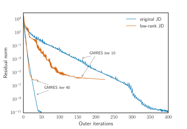
Fig. 1: Residual norm w.r.t. the number of outer iterations for the original and the proposed JD methods. Plots are done for different number of inner GMRES iterations to solve linear systems. Parameters: $N=150^{2}$, $r=5$.

We note that the cost of each inner iteration is different: $\mathcal{O}(nrR)$ for the proposed version and $\mathcal{O}(n^{2})$ for the original version, so the proposed version is more efficient for large $n$. Nevertheless, Figure 1 shows that our method requires fewer number of less expensive iterations to achieve a given accuracy (before stagnation). The less accurately we solve the system, the more gain we observe. Such speed-up may happen due to the usage of additional information about the solution, namely that it is of low rank.

Comparison with the low-rank Davidson approach and the Rayleigh quotient iteration

In this experiment we compare performance of the proposed fixed-rank Jacobi-Davidson approach and the proposed Rayleigh quotient inverse iteration (29). We also compare them with the “Davidson” approach when no projection $I-x_{k}x_{k}^{\top}$ is done:

$$\left[\mathrm{P}_{T_{X_{k}}\mathcal{M}_{r}}(A-\mathfrak{R}(x_{k})I)\mathrm{P}_{T_{X_{k}}\mathcal{M}_{r}}\right]\xi_{k}=-\mathrm{P}_{T_{X_{k}}\mathcal{M}_{r}}r_{k},\quad\mathrm{P}_{T_{X_{k}}\mathcal{M}_{r}}\xi_{k}=\xi_{k}.$$ (36)

Figure 2 illustrates the results of the comparison. As anticipated, when local systems are solved accurately the Davidson approach stagnates since the exact solution of (36) is $-x_{k}$. So, no additional information is added to the previous approximation $x_{k}$. This problem does not occur if local systems are solved inexactly. For the Rayleigh quotient iteration we observe opposite behaviour due to the deterioration of condition number of local systems. The Jacobi-Davidson approach yields good convergence in both cases.

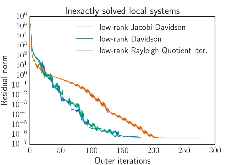
(a)

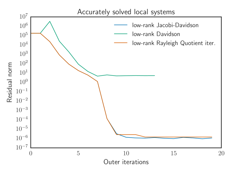
(b)

Fig. 2: Residual w.r.t. number of outer iterations, $N=2000^{2}$, $r=3$. Local systems from Figure 2(a) were solved inexactly using $100$ GMRES iterations, while local systems from Figure 2(b) were solved accurately with the preconditioner (35), $K=20$ and $30$ GMRES iterations.

Comparison with the ALS method

Alternating linear scheme (ALS) method is the standard approach for low-rank optimization. The idea is following: given $X=UV^{\top}$ we minimize Rayleigh quotient $\mathfrak{R}(x)\equiv\widetilde{\mathfrak{R}}(U,V)$ successively over $U$ and $V$. Minimization over $U$ results in the eigenvalue problem with matrix $A_{v,v}$, while minimization over $V$ results in the eigenvalue problem with matrix $A_{u,u}$.

Note that in the proposed JD method we need to solve local systems, while in the ALS approach we solve local eigenvalue problems. To make comparison fair we ran original JD method to solve local problems in ALS. We choose the fixed number of iterations as choosing fixed accuracy to solve eigenvalue problems in ALS leads to stagnation of the method. Since the inner JD solver has two types of iterations: iterations to solve local problem and outer iterations, we need to tune these parameters to get fair comparison. We tuned them such that each ALS iteration runs approximately the same amount of time as the outer iteration of the proposed JD and gives the best possible convergence. Results are presented on Figure 3. On both subfigures the proposed JD method yields the fastest convergence.

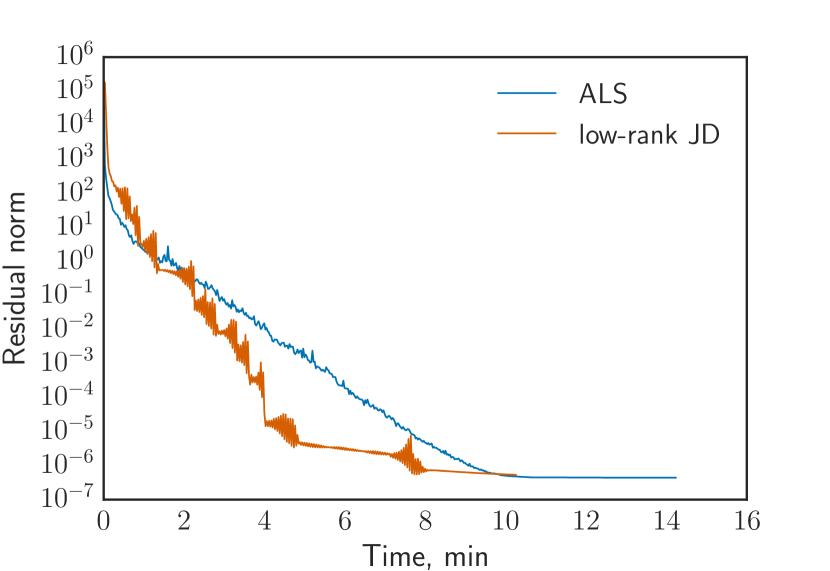
(a)

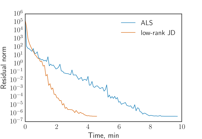
(b)

Fig. 3: Residual w.r.t. time for ALS and the proposed JD methods. Figures 3(a) and 3(b) correspond to 150 and 600 GMRES iterations to solve local problem of the proposed JD. Parameters of local problems in ALS were chosen to give similar to the proposed JD time of each outer iteration, $N=2000^{2}$.

Subspace acceleration

In this part we investigate the behaviour of the subspace accelerated version proposed in Sec. 4. First, on Figure 5 we compare he original subspace acceleration and the version with vector transport when subspace is projected onto the tangent space of the current approximation. No restarts are used. As anticipated the projected version stagnates when accuracy of approximation equals error of low-rank approximation. Apart from that, the convergence behaviour of the methods is comparable, but the projected version is more suitable for low-rank calculations. To illustrate this point we provide Figure 5, where the projected version is compared with the version with no projection. The latter one is implemented with hard rank thresholding of linear combination (20). No additional optimization over coefficients besides Rayleigh-Ritz procedure is done. As we observe from the figure, the projected version outperforms the version without projection. The point is that we exactly optimize coefficients on the tangent space since no rank thresholding in this case is required. If vectors do not belong to the tangent space, rank rapidly grows with the subspace size and rank thresholding can introduce significant error.

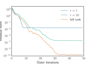
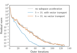
Fig. 4: Comparison of original subspace accelerated version of JD and the version with vector transport. In both cases full version of JD with no restarts is used. $N=150^{2}$, local systems are solved using $150$ GMRES iterations.

Fig. 5: Proposed JD method with subspace acceleration for two cases: when search subspace is projected onto the tangent space (with vector transport) and when no projection is done. Parameters: $N=2000^{2}$, $r=5$, $150$ GMRES iterations to solve local systems.

9 Related work

Eigenvalue problems with low-rank constraint are usually considered in literature in the context of more general low-rank decompositions of multidimensional arrays, e.g. the tensor train decomposition [22]. Two-dimensional case naturally follows from the multidimensional generalization.

There are two standard ways to solve eigenvalue problems in low-rank format: optimization of Rayleigh quotient based on alternating minimization, which accounts for multilinear structure of the decomposition, and iterative methods with rank truncation. The first approach has been developed for a long time in the matrix product state community [25, 28, 23]. We also should mention altenating minimization algorithms that were recently proposed in the mathematical community. They are based either on the alternating linear scheme (ALS) procedure [11, 7] or on basis enrichment using alternating minimal energy method (AMEn) [14, 8]. Rank truncated iterative methods include power method [4, 5], inverse iteration [10], locally optimal block preconditioned conjugate gradient method [15, 17, 18]. For more information about eigensolvers in low-rank formats see [9]. To our knowledge no generalization of the Jacobi-Davidson method was considered.

In [16] authors consider inexact Riemannian Newton method for solving linear systems with a low-rank solution. They also omit the curvature part in the Hessian and utilize specific structure of the operator to construct a preconditioner.

In [24] authors proposed a version of inverse iteration based on the alternating linear scheme ALS procedure, which is similar to (28). By contrast, the present work considers inverse iteration on the whole tangent space. We also provide an interpretation of the method as an inexact Newton method.

We note that the proposed approach is considered on the fixed rank manifolds. Recently desingularization technique was applied to non-smooth variety of bounded-rank matrices $\mathcal{M}_{\leq r}$ [13].

10 Conclusions and future work

The natural next step is to consider generalization to the multidimensional case. Most of the results can be directly generalized to the tensor train decomposition, e.g. (17), (20) and (29). However, to avoid cumbersome formulas and present the method in the most comprehensible way we restricted the paper to the treatment of the two-dimensional case. Moreover, the correct choice of parametrization of the tangent space and efficient practical implementation worth individual consideration. We plan to address them in a separate work and test the method on real-world applications.

References

- [1] P-A Absil, Robert Mahony, and Rodolphe Sepulchre. Optimization algorithms on matrix manifolds. Princeton University Press, 2009.
- [2] P-A Absil, Robert Mahony, and Jochen Trumpf. An extrinsic look at the riemannian hessian. In Geometric science of information, pages 361–368. Springer, 2013.
- [3] P. A. Absil and I. V. Oseledets. Low-rank retractions: a survey and new results. Comput. Optim. Appl., 2014.
- [4] G. Beylkin and M. J. Mohlenkamp. Numerical operator calculus in higher dimensions. Proc. Nat. Acad. Sci. USA, 99(16):10246–10251, 2002.
- [5] G. Beylkin and M. J. Mohlenkamp. Algorithms for numerical analysis in high dimensions. SIAM J. Sci. Comput., 26(6):2133–2159, 2005.
- [6] Ernest R. Davidson. The iterative calculation of a few of the lowest eigenvalues and corresponding eigenvectors of large real-symmetric matrices. J. Comput. Phys., 17(1):87–94, 1975.
- [7] S. V. Dolgov, B. N. Khoromskij, I. V. Oseledets, and D. V. Savostyanov. Computation of extreme eigenvalues in higher dimensions using block tensor train format. Computer Phys. Comm., 185(4):1207–1216, 2014.
- [8] S. V. Dolgov and D. V. Savostyanov. Corrected one-site density matrix renormalization group and alternating minimal energy algorithm. In Numerical Mathematics and Advanced Applications — ENUMATH 2013, volume 103, pages 335–343, 2015.
- [9] L. Grasedyck, D. Kressner, and C. Tobler. A literature survey of low-rank tensor approximation techniques. GAMM-Mitt., 36(1):53–78, 2013.
- [10] W. Hackbusch, B. N. Khoromskij, S. A. Sauter, and E. E. Tyrtyshnikov. Use of tensor formats in elliptic eigenvalue problems. Numer. Linear Algebra Appl., 19(1):133–151, 2012.
- [11] S. Holtz, T. Rohwedder, and R. Schneider. The alternating linear scheme for tensor optimization in the tensor train format. SIAM J. Sci. Comput., 34(2):A683–A713, 2012.
- [12] B. N. Khoromskij. Tensor-structured preconditioners and approximate inverse of elliptic operators in . Constr. Approx., 30:599–620, 2009.
- [13] Valentin Khrulkov and Ivan Oseledets. Desingularization of bounded-rank matrix sets. arXiv preprint 1612.03973, 2016.
- [14] D. Kressner, M. Steinlechner, and A. Uschmajew. Low-rank tensor methods with subspace correction for symmetric eigenvalue problems. SIAM J Sci. Comput., 36(5):A2346–A2368, 2014.
- [15] D. Kressner and C. Tobler. Preconditioned low-rank methods for high-dimensional elliptic PDE eigenvalue problems. Computational Methods in Applied Mathematics, 11(3):363–381, 2011.
- [16] Daniel Kressner, Michael Steinlechner, and Bart Vandereycken. Preconditioned low-rank Riemannian optimization for linear systems with tensor product structure. SIAM J. Sci. Comput., 38(4):A2018–A2044, 2016.
- [17] O. S. Lebedeva. Block tensor conjugate gradient-type method for Rayleigh quotient minimization in two-dimensional case. Comput. Math. Math. Phys., 50(5):749–765, 2010.
- [18] O. S. Lebedeva. Tensor conjugate-gradient-type method for Rayleigh quotient minimization in block QTT-format. Russ. J. Numer. Anal. Math. Modelling, 26(5):465–489, 2011.
- [19] John M. Lee. Introduction to smooth manifolds, 2001.
- [20] Yvan Notay. Combination of Jacobi–Davidson and conjugate gradients for the partial symmetric eigenproblem. Numer. Linear Algebra Appl., 9(1):21–44, 2002.
- [21] Yvan Notay. Inner iterations in eigenvalue solvers. Report GANMN 05, 1, 2005.
- [22] I. V. Oseledets. Tensor-train decomposition. SIAM J. Sci. Comput., 33(5):2295–2317, 2011.
- [23] S. Östlund and S. Rommer. Thermodynamic limit of density matrix renormalization. Phys. Rev. Lett., 75(19):3537–3540, 1995.
- [24] Maxim Rakhuba and Ivan Oseledets. Calculating vibrational spectra of molecules using tensor train decomposition. J. Chem. Phys., 145:124101, 2016.
- [25] U. Schollwöck. The density-matrix renormalization group in the age of matrix product states. Annals of Physics, 326(1):96–192, 2011.
- [26] Gerard L. G. Sleijpen and Henk A. Van der Vorst. A Jacobi–Davidson iteration method for linear eigenvalue problems. SIAM Rev., 42(2):267–293, 2000.
- [27] Bart Vandereycken. Low-rank matrix completion by Riemannian optimization. SIAM J. Optim., 23(2):1214–1236, 2013.
- [28] Steven R. White. Density matrix formulation for quantum renormalization groups. Phys. Rev. Lett., 69(19):2863–2866, 1992.