Diving into the shallows: a computational perspective on large-scale shallow learning

Abstract

Remarkable recent success of deep neural networks has not been easy to analyze theoretically. It has been particularly hard to disentangle relative significance of architecture and optimization in achieving accurate classification on large datasets. On the other hand, shallow methods (such as kernel methods) have encountered obstacles in scaling to large data, despite excellent performance on smaller datasets, and extensive theoretical analysis. Practical large-scale optimization methods, such as variants of gradient descent, used so successfully in deep learning, seem to produce below par results when applied to kernel methods.

In this paper we first identify a basic limitation in gradient descent-based optimization methods when used in conjunctions with smooth kernels. An analysis based on the spectral properties of the kernel demonstrates that only a vanishingly small portion of the function space is reachable after a polynomial number of gradient descent iterations. This lack of approximating power drastically limits gradient descent for a fixed computational budget leading to serious over-regularization/underfitting. The issue is purely algorithmic, persisting even in the limit of infinite data.

To address this shortcoming in practice, we introduce EigenPro iteration, based on a simple and direct preconditioning scheme using a small number of approximately computed eigenvectors. It can also be viewed as learning a new kernel optimized for gradient descent. It turns out that injecting this small (computationally inexpensive and SGD-compatible) amount of approximate second-order information leads to major improvements in convergence. For large data, this translates into significant performance boost over the standard kernel methods. In particular, we are able to consistently match or improve the state-of-the-art results recently reported in the literature with a small fraction of their computational budget.

Finally, we feel that these results show a need for a broader computational perspective on modern large-scale learning to complement more traditional statistical and convergence analyses. In particular, many phenomena of large-scale high-dimensional inference are best understood in terms of optimization on infinite dimensional Hilbert spaces, where standard algorithms can sometimes have properties at odds with finite-dimensional intuition. A systematic analysis concentrating on the approximation power of such algorithms within a budget of computation may lead to progress both in theory and practice.

1 Introduction

In recent years we have witnessed remarkable advances in many areas of artificial intelligence. In large part this progress has been due to the success of machine learning methods, notably deep neural networks, applied to very large datasets. These networks are typically trained using variants of stochastic gradient descent (SGD), allowing training on large data using modern hardware. Despite intense recent research and significant progress toward understanding SGD and deep architectures, it has not been easy to understand the underlying causes of that success. Broadly speaking, it can be attributed to (a) the structure of the function space represented by the network or (b) the properties of the optimization algorithms used. While these two aspects of learning are intertwined, they are distinct and there is hope that they may be disentangled.

As learning in deep neural networks is still largely resistant to theoretical analysis, progress both in theory and practice can be made by exploring the limits of shallow methods on large datasets. Shallow methods, such as kernel methods, are a subject of an extensive and diverse literature. Theoretically, kernel machines are known to be universal learners, capable of learning nearly arbitrary functions given a sufficient number of examples [STC04, SC08]. Kernel methods are easily implementable and show state-of-the-art performance on smaller datasets (see [CK11, HAS⁺14, DXH⁺14, LML⁺14, MGL⁺17] for some comparisons with DNN’s). On the other hand, there has been significantly less progress in applying these methods to large modern data. The goal of this work is to make a step toward understanding the subtle interplay between architecture and optimization for shallow algorithms and to take practical steps to improve performance of kernel methods on large data.

The paper consists of two main parts. First, we identify a basic underlying limitation of using gradient descent-based methods in conjunction with smooth kernels typically used in machine learning. We show that only very smooth functions can be well-approximated after polynomially many steps of gradient descent. On the other hand, a less smooth target function cannot be approximated within $\epsilon$ using any polynomial number $P(1/\epsilon)$ steps of gradient descent for kernel regression. This phenomenon is a result of the fast spectral decay of smooth kernels and can be readily understood in terms of the spectral structure of the gradient descent operator in the least square regression/classification setting, which is the focus of our discussion. Note the marked contrast with the standard analysis of gradient descent for convex optimizations problems, requiring at most $O(1/\epsilon)$ steps to get an $\epsilon$-approximation of a minimum. The difference is due to the infinite (or, in practice, very high) dimensionality of the target space and the fact that the minimizer of a convex functional is not generally an element of the same space.

A direct consequence of this theoretical analysis is slow convergence of gradient descent methods for high-dimensional regression, resulting in severe over-regularization/underfitting and suboptimal performance for less smooth functions. These functions are arguably very common in practice, at least in the classification setting, where we expect sharp transitions or even discontinuities near the class boundaries. We give some examples on real data showing that the number of steps of gradient descent needed to obtain near-optimal classification is indeed very large even for smaller problems. This shortcoming of gradient descent is purely algorithmic and is not related to the sample complexity of the data, persisting even in the limit of infinite data. It is also not an intrinsic flaw of kernel architectures, which are capable of approximating arbitrary functions but potentially require a very large number of gradient descent steps. The issue is particularly serious for large data, where direct second order methods cannot be used due to the computational constraints. Indeed, even for a dataset with only $10^{6}$ data points, practical direct solvers require cubic, on the order of $10^{18}$ operations, weeks of computational time for a fast processor/GPU. While many approximate second-order methods are available, they rely on low-rank approximations and, as we discuss below, also lead to over-regularization as important information is contained in eigenvectors with very small eigenvalues typically discarded in such approximations.

In the second part of the paper we address this problem by proposing EigenPro iteration (see github.com/EigenPro for the code), a direct and simple method to alleviate slow convergence resulting from fast eigen-decay for kernel (and covariance) matrices. EigenPro is a preconditioning scheme based on approximately computing a small number of top eigenvectors to modify the spectrum of these matrices. It can also be viewed as constructing a new kernel, specifically optimized for gradient descent. While EigenPro uses approximate second-order information, it is only employed to modify first-order gradient descent leading to the same mathematical solution (without introducing a bias). Moreover, only one second-order problem at the start of the iteration needs to be solved. EigenPro requires only a small overhead per iteration compared to standard gradient descent and is also fully compatible with SGD. We analyze the step size in the SGD setting and provide a range of experimental results for different kernels and parameter settings showing consistent acceleration by a factor from five to over thirty over the standard methods, such as Pegasos [SSSSC11] for a range of datasets and settings. For large datasets, when the computational budget is limited, that acceleration translates into significantly improved accuracy and/or computational efficiency. It also obviates the need for complex computational resources such as supercomputer nodes or AWS clusters typically used with other methods. In particular, we are able to improve or match the state-of-the-art recent results for large datasets in the kernel literature at a small fraction of their reported computational budget, using a single GPU.

Finally, we note that in the large data setting, we are limited to a small number of iterations of gradient descent and certain approximate second-order computations. Thus, investigations of algorithms based on the space of functions that can be approximated within a fixed computational budget of these operations (defined in terms of the input data size) reflect the realities of modern large-scale machine learning more accurately than the more traditional analyses of convergence rates. Moreover, many aspects of modern inference are best reflected by an infinite dimensional optimization problem whose properties are sometimes different from the standard finite-dimensional results. Developing careful analyses and insights into these issues will no doubt result in significant pay-offs both in theory and in practice.

2 Gradient descent for shallow methods

Shallow methods. In the context of this paper, shallow methods denote the family of algorithms consisting of a (linear or non-linear) feature map $\operatorname{\phi}:\mathbb{R^{N}}\to\mathcal{H}$ to a (finite or infinite-dimensional) Hilbert space $\mathcal{H}$ followed by a linear regression/classification algorithm. This is a simple yet powerful setting amenable to theoretical analysis. In particular, it includes the class of kernel methods, where the feature map typically takes us from finite dimensional input to an infinite dimensional Reproducing Kernel Hilbert Space (RKHS). In what follows we will employ the square loss which significantly simplifies the analysis and leads to efficient and competitive algorithms.

Linear regression. Consider $n$ labeled data points $\{({\boldsymbol{x}}_{1},y_{1}),...,({\boldsymbol{x}}_{n},y_{n})\in\mathcal{H}\times\mathbb{R}\}$. To simplify the notation let us assume that the feature map has already been applied to the data, i.e., ${\boldsymbol{x}}_{i}=\operatorname{\phi}({\boldsymbol{z}}_{i})$. Least square linear regression aims to recover the parameter vector $\alpha^{*}$ that minimize the empirical loss as follows:

$$L({\boldsymbol{\alpha}})\mathrel{\overset{\makebox[0.0pt]{\mbox{\tiny def}}}{=}}\frac{1}{n}\sum_{i=1}^{n}(\langle{\boldsymbol{\alpha}},{\boldsymbol{x}}_{i}\rangle_{\mathcal{H}}-y_{i})^{2}$$ (1)

$${\boldsymbol{\alpha}}^{*}=\arg\min_{{\boldsymbol{\alpha}}\in{\mathcal{H}}}{L({\boldsymbol{\alpha}})}$$ (2)

When ${\boldsymbol{\alpha}}^{*}$ is not uniquely defined, we can choose the smallest norm solution. We do not include the typical regularization term, $\lambda\|\alpha\|_{\mathcal{H}}^{2}$ for reasons which will become clear shortly.

Minimizing the empirical loss is related to solving a linear system of equations. Define the data matrix $X\mathrel{\overset{\makebox[0.0pt]{\mbox{\tiny def}}}{=}}({\boldsymbol{x}}_{1},...,{\boldsymbol{x}}_{n})^{T}$ and the label vector ${\boldsymbol{y}}\mathrel{\overset{\makebox[0.0pt]{\mbox{\tiny def}}}{=}}(y_{1},...,y_{n})^{T}$, as well as the (non-centralized) covariance matrix/operator,

$$H\mathrel{\overset{\makebox[0.0pt]{\mbox{\tiny def}}}{=}}\frac{2}{n}\sum_{i=1}^{n}{{\boldsymbol{x}}_{i}{\boldsymbol{x}}_{i}^{T}}=\frac{2}{n}X^{T}X$$ (3)

Rewrite the loss as $L({\boldsymbol{\alpha}})=\frac{1}{n}\left\lVert X{\boldsymbol{\alpha}}-{\boldsymbol{y}}\right\rVert^{2}_{2}$. Since $\nabla L({\boldsymbol{\alpha}})\mid_{{\boldsymbol{\alpha}}={\boldsymbol{\alpha}}^{*}}=0$, minimizing $L({\boldsymbol{\alpha}})$ is equivalent to solving the linear system

$$H{\boldsymbol{\alpha}}-{\boldsymbol{b}}=0$$ (4)

with ${\boldsymbol{b}}=X^{T}{\boldsymbol{y}}$. When $d=\dim({\mathcal{H}})<\infty$, the time complexity of solving the linear system in Eq. 4 directly (using Gaussian elimination or other methods typically employed in practice) is $O(d^{3})$.

Remark 2.1.

For kernel methods we frequently have $d=\infty$. Instead of solving Eq. 4, one solves the dual $n\times n$ system $K{\boldsymbol{\alpha}}-{\boldsymbol{y}}=0$ where $K\mathrel{\overset{\makebox[0.0pt]{\mbox{\tiny def}}}{=}}[k({\boldsymbol{z}}_{i},{\boldsymbol{z}}_{j})]_{i,j=1,\ldots,n}$ is the kernel matrix corresponding to the kernel function $k(\cdot,\cdot)$. The solution can be written as $\sum_{i=1}^{n}k({\boldsymbol{z}}_{i},\cdot){\boldsymbol{\alpha}}({\boldsymbol{z}}_{i})$. A direct solution requires $O(n^{3})$ operations.

Gradient descent (GD). While linear systems of equations can be solved by direct methods, their computational demands make them impractical for large data. On the other hand, gradient descent-type iterative methods hold the promise of a small number of $O(n^{2})$ matrix-vector multiplications, a much more manageable task. Moreover, these methods can typically be used in a stochastic setting, reducing computational requirements and allowing for very efficient GPU implementations. These schemes are adopted in popular kernel methods implementations such as NORMA [KSW04], SDCA [HCL⁺08], Pegasos [SSSSC11], and DSGD [DXH⁺14].

For linear systems of equations gradient descent takes a particularly simple form known as Richardson iteration [Ric11]. It is given by

$${\boldsymbol{\alpha}}^{(t+1)}={\boldsymbol{\alpha}}^{(t)}-\eta(H{\boldsymbol{\alpha}}^{(t)}-{\boldsymbol{b}})$$ (5)

We see that

$${\boldsymbol{\alpha}}^{(t+1)}-{\boldsymbol{\alpha}}^{*}=({\boldsymbol{\alpha}}^{(t)}-{\boldsymbol{\alpha}}^{*})-\eta H({\boldsymbol{\alpha}}^{(t)}-{\boldsymbol{\alpha}}^{*})$$

and thus

$${\boldsymbol{\alpha}}^{(t+1)}-{\boldsymbol{\alpha}}^{*}=(I-\eta H)^{t}({\boldsymbol{\alpha}}^{(1)}-{\boldsymbol{\alpha}}^{*})$$ (6)

It is easy to see that for convergence of ${\boldsymbol{\alpha}}^{t}$ to ${\boldsymbol{\alpha}}^{*}$ as $t\to\infty$ we need to ensure that $\|I-\eta H\|\leq 1$. It follows that $0<\eta<2/\lambda_{1}(H)$.

Remark 2.2.

When $H$ is finite dimensional the inequality has to be strict. In infinite dimension convergence is possible even if $\|I-\eta H\|=1$ as long as each eigenvalue of $I-\eta H$ is strictly smaller than one in absolute value. That will be the case for kernel integral operators.

It is now easy to describe the computational reach of gradient descent $\mathcal{CR}_{t}$, i.e. the set of vectors which can be $\epsilon$-approximated by gradient descent after $t$ steps

$$\mathcal{CR}_{t}(\epsilon)\mathrel{\overset{\makebox[0.0pt]{\mbox{\tiny def}}}{=}}\{{\boldsymbol{v}}\in{\mathcal{H}},s.t.\|(I-\eta H)^{t}{\boldsymbol{v}}\|<\epsilon\|{\boldsymbol{v}}\|\}$$

It is important to note that any ${\boldsymbol{b}}\notin\mathcal{CR}_{t}(\epsilon)$ cannot be $\epsilon$-approximated by gradient descent in less than $t+1$ iterations.

Remark 2.3.

We typically care about the quality of the solution $\|H{\boldsymbol{\alpha}}^{(t)}-{\boldsymbol{b}}\|$, rather than the error estimating the parameter vector $\|{\boldsymbol{\alpha}}^{(t)}-{\boldsymbol{\alpha}}^{*}\|$ where ${\boldsymbol{\alpha}}^{*}=H^{-1}{\boldsymbol{b}}$. Thus (noticing that $H$ and $(I-\eta H)^{t}$ commute), we get $\|(I-\eta H)^{t}{\boldsymbol{v}}\|=\|H^{-1}(I-\eta H)^{t}H{\boldsymbol{v}}\|$ in the definition.

Remark 2.4 (Initialization).

We assume that the initialization ${\boldsymbol{\alpha}}^{(1)}=0$. Choosing a different starting point will not significantly change the analysis unless second order information is incorporated in the initialization conditions. We also note that if $H$ is not full rank, gradient descent will converge to the minimum norm solution of Eq. 4.

Remark 2.5 (Infinite dimensionality).

Some care needs to be taken when $K$ is infinite-dimensional. In particular, the space of parameters $\alpha=K^{-1}{\mathcal{H}}$ and ${\mathcal{H}}$ are very different spaces when $K$ is an integral operator. The space of parameters is in fact a space of distributions (generalized functions). Sometimes that can be addressed by using $K^{1/2}$ instead of $K$, as $K^{-1/2}{\mathcal{H}}=L^{2}(\Omega)$.

To get a better idea of the space $\mathcal{CR}_{t}(\epsilon)$ consider the eigendecomposition of $H$. Let $\lambda_{1}\geq\lambda_{2}\geq\ldots\geq 0$ be its eigenvalues and ${\boldsymbol{e}}_{1},{\boldsymbol{e}}_{2},\ldots$ the corresponding eigenvectors/eigenfunctions. We have

$$H=\sum{\lambda_{i}{\boldsymbol{e}}_{i}{\boldsymbol{e}}_{i}^{T}},\leavevmode\nobreak\ \leavevmode\nobreak\ \leavevmode\nobreak\ \leavevmode\nobreak\ \langle{\boldsymbol{e}}_{i},{\boldsymbol{e}}_{j}\rangle=\delta_{ij}$$ (7)

Writing Eq. 6 in terms of eigendirection yields

$${\boldsymbol{\alpha}}^{(t+1)}-{\boldsymbol{\alpha}}^{*}=\sum{(1-\eta\lambda_{i})^{t}\langle{\boldsymbol{e}}_{i},{\boldsymbol{\alpha}}^{(1)}-{\boldsymbol{\alpha}}^{*}\rangle{\boldsymbol{e}}_{i}}$$ (8)

and hence, putting $a_{i}=\langle{\boldsymbol{e}}_{i},{\boldsymbol{v}}\rangle$,

$$\mathcal{CR}_{t}(\epsilon)=\{{\boldsymbol{v}},s.t.\sum{(1-\eta\lambda_{i})^{2t}a_{i}^{2}}<\epsilon^{2}\sum a_{i}^{2}$$ (9)

Recalling that $\eta<2\lambda_{1}$ and using the fact that $(1-1/z)^{z}\approx 1/e$, we see that a necessary condition for ${\boldsymbol{v}}\in\mathcal{CR}_{t}$

$$\frac{1}{3}\sum_{i,s.t.\lambda_{i}<\frac{\lambda_{1}}{2t}}a_{i}^{2}<\sum_{i}{(1-\eta\lambda_{i})^{2t}a_{i}^{2}}<\epsilon^{2}\sum a_{i}^{2}$$ (10)

This is a convenient characterization, we will denote

$$\mathcal{CR^{\prime}}_{t}(\epsilon)\mathrel{\overset{\makebox[0.0pt]{\mbox{\tiny def}}}{=}}\{{\boldsymbol{v}},s.t.\sum_{i,s.t.\lambda_{i}<\frac{\lambda_{1}}{2t}}a_{i}^{2}<\epsilon^{2}\ \|{\boldsymbol{v}}\|^{2}\supset\mathcal{CR}_{t}(\epsilon)$$ (11)

Another convenient necessary condition for ${\boldsymbol{v}}\in\mathcal{CR}_{t}$, is that

$$\forall_{i}\leavevmode\nobreak\ \leavevmode\nobreak\ \leavevmode\nobreak\ \left|{\left(1-\frac{2\lambda_{i}}{\lambda_{1}}\right)^{t}\langle{\boldsymbol{e}}_{i},{\boldsymbol{v}}\rangle}\right|<\epsilon\|{\boldsymbol{v}}\|.$$

Applying logarithm and noting that $\log(1-x)<-x$ results in the following inequality that must hold for all $i$ (assuming $\lambda_{i}<\lambda_{1}/2$):

$$t>\frac{\lambda_{1}}{2\lambda_{i}}\log\left(\frac{|\langle{\boldsymbol{e}}_{i},{\boldsymbol{v}}\rangle|}{\epsilon\|{\boldsymbol{v}}\|}\right)$$ (12)

Remark 2.6.

The standard result (see, e.g., [BV04]) that the number of iterations necessary for uniform convergence is of the order of the condition number $\lambda_{1}/\lambda_{d}$ follows immediately. However, we are primarily interested in the case when $d$ is infinite or very large. The corresponding operators/matrices are extremely ill-conditioned with infinite or approaching infinity condition number. In that case instead of a single condition number, one should consider a sequence of “condition numbers” along each eigen-direction.

2.1 Gradient descent, smoothness, and kernel methods.

We now proceed to analyze the computational reach for kernel methods. We will start by discussing the case of infinite data (the population case). It is both easier to analyze and allows us to demonstrate the purely computational (non-statistical) nature of limitations of gradient descent.

We will show that when the kernel is smooth, the reach of gradient descent is limited to very smooth, at least infinitely differentiable functions. Moreover, to approximate a function with less smoothness within some accuracy $\epsilon$ in the $L^{2}$ norm one needs a super-polynomial (or even exponential) in $1/\epsilon$ number of iterations of gradient descent.

Let the data be sampled from a probability with density $\mu$ on a compact domain $\Omega\subset\mathbb{R}^{p}$. In the case of infinite data $\mathcal{K}$ becomes an integral operator corresponding to a positive definite kernel $k(\cdot,\cdot)$. We have

$$\mathcal{K}f(x)=\int_{\Omega}k(x,z)f(z)d\mu_{z}$$ (13)

This is a compact self-adjoint operator with an infinite positive spectrum $\lambda_{1},\lambda_{2},\ldots$ with $\lim_{i\rightarrow\infty}\lambda_{i}=0$.

We start by stating some results on the decay of eigenvalues of $\mathcal{K}$.

Theorem 1.

If $k$ is an infinitely differentiable kernel, the rate of eigenvalue decay is super-polynomial, i.e.

$$\lambda_{i}=O(i^{-P})\leavevmode\nobreak\ \leavevmode\nobreak\ \leavevmode\nobreak\ \leavevmode\nobreak\ \leavevmode\nobreak\ \forall P\in\mathbb{N}$$

Moreover, if $k$ is an infinitely differentiable radial kernel (e.g., a Gaussian kernel), there exist constants $C,C^{\prime}>0$ such that for large enough $i$,

$$\lambda_{i}<C^{\prime}\exp\left(-C{i^{1/p}}\right)$$

Proof.

The statement for arbitrary smooth kernels is an immediate corollary of Theorem 4 in [Küh87]. The rate for the practically important smooth radial kernels, including Gaussian kernels, Cauchy kernel and a number of other kernel families, is given in in [SS16], Theorem 6. ∎

Remark 2.7.

Interestingly, while eigenvalue decay is nearly exponential, it becomes milder as the dimension increases, leading to an unexpected “blessing of dimensionality" for gradient-descent type methods in high dimension. On the other hand, while not reflected in Theorem 1, this depends on the intrinsic dimension of the data, moderating the effect.

The computational reach of gradient descent in kernel methods. Consider now the eigenfunctions of $\mathcal{K}$, $\mathcal{K}e_{i}=\lambda_{i}e_{i}$, which form an orthonormal basis for $L^{2}(\Omega)$ by the Mercer’s theorem. We can write a function $f\in L^{2}(\Omega)$ as $f=\sum_{i=1}^{\infty}a_{i}e_{i}$. We have $\|f\|_{L^{2}}^{2}=\sum_{i=1}^{\infty}a_{i}^{2}$.

We can now describe the reach of kernel methods with smooth kernel (in the infinite data setting). Specifically, functions which can be approximated in a polynomial number of iterations must have super-polynomial coefficient decay in the basis of kernel eigenfunctions.

Theorem 2.

Suppose $f\in L^{2}(\Omega)$ is such that it can be approximated within $\epsilon$ using a polynomial in $1/\epsilon$ number of gradient descent iterations, i.e., $\forall_{\epsilon>0}f\in\mathcal{CR}_{\epsilon^{-M}}(\epsilon)$ for some $M\in\mathbb{N}$. Then for any $N\in\mathbb{N}$ and $i$ large enough $|a_{i}|<i^{-N}$.

Proof.

Note that $f\in{CR^{\prime}}_{t}(\epsilon)$. We have $1/3\sum_{i,s.t.\lambda_{i}<\frac{\lambda_{1}}{2\epsilon^{M}}}a_{i}^{2}<\epsilon^{2}\|f\|$ and hence $|a_{i}|<\sqrt{3}\epsilon\|f\|$ for any $i$, such that $\lambda_{i}<\frac{\lambda_{1}}{2\epsilon^{M}}$. From Theorem 1 we have $\lambda_{i}=o(i^{-NM})$. Thus this inequality holds whenever $i>C\epsilon^{-1/N}$ for some $C$. Writing $\epsilon$ in terms of $i$ yields $|a_{i}|<i^{-N}$ for $i$ sufficiently large. ∎

It is easy to see that the eigenfunctions $e_{i}$ corresponding to an infinitely differentiable kernel are also infinitely differentiable. Suppose in addition that their derivatives grow at most polynomially in $i$, i.e. $\|e_{i}\|_{W_{k,2}}<P_{k}(i)$, where $P_{k}$ is some polynomial and $W_{k,2}$ is a Sobolev space. Then by differentiating the expansion of $f$ in terms of eigenfunctions we have the following

Corollary 1.

Any $f\in L^{2}(\Omega)$ that for any $\epsilon>0$ can be $\epsilon$-approximated with polynomial in $1/\epsilon$ number of steps of gradient descent is infinitely differentiable. Thus, if $f$ is not infinitely differentiable it cannot be $\epsilon$-approximated in $L^{2}(\Omega)$ using a polynomial number of gradient descent steps.

We contrast Theorem 2 showing extremely slow convergence of gradient descent with the analysis of gradient descent for convex objective functions. The standard analysis (e.g. [B⁺15]) indicates that $O(1/\epsilon)$ steps of gradient descent is sufficient to recover the optimal value with $\epsilon$ accuracy and at first glance seems to apply in general to infinite dimensional Hilbert spaces. However in this case the standard analysis cannot be used is that the sequence ${\boldsymbol{\alpha}}^{(t)}$ diverges in $L^{2}(\Omega)$ as the optimal solution $f^{*}=\mathcal{K}^{-1}\mathrm{y}$ is not generally a function in $L^{2}(\Omega)$. This is a consequence of the fact that the infinite-dimensional operator $\mathcal{K}^{-1}$ is unbounded (see Appendix D for some experimental results).

Remark 2.8.

Note that in finite dimension every non-degenerate operator, e.g. an inverse of a kernel matrix, is bounded. Nevertheless, infinite dimensional unboundedness manifests itself as the norm of the optimal solution can increase very rapidly with the size of the kernel matrix.

Gradient descent for periodic functions on $\mathbb{R}$. Let us now consider a simple but important special case, where gradient descent and its reach can be analyzed very explicitly. Let $\Omega$ be a circle with the uniform measure, or, equivalently, consider periodic functions on the interval $[0,2\pi]$. Let $k_{s}(x,z)$ be the heat kernel on the circle [Ros97]. This kernel is very close to the Gaussian kernel $k_{s}(x,z)\approx\frac{1}{\sqrt{2\pi s}}\exp{\left(-\frac{(x-z)^{2}}{4s}\right)}$. The eigenfunctions $e_{j}$ of the integral operator $\mathcal{K}$ corresponding to $k_{s}(x,z)$ are simply the Fourier harmonics $\sin jx$ and $\cos jx$. The corresponding eigenvalues are $\{1,e^{-s},e^{-s},e^{-4s},e^{-4s},\ldots,e^{-\lfloor j/2+1\rfloor^{2}s},\ldots\}$ and the kernel can be written as

$$k_{s}(x,z)=\sum_{0}^{\infty}e^{-\lfloor j/2+1\rfloor^{2}s}e_{j}(x)e_{j}(z).$$

Given a function $f$ on $[0,2\pi]$, we can write its Fourier series $f=\sum_{j=0}^{\infty}a_{j}e_{j}$. A direct computation shows that for any $f\in{CR}_{t}(\epsilon)$, we have $\sum_{i>\frac{\sqrt{2\ln{2t}}}{s}}a_{i}^{2}<3\epsilon^{2}\sum_{0}^{\infty}a_{i}^{2}$. We see that the space $f\in{CR}_{t}(\epsilon)$ is “frozen” as ${\sqrt{2\ln{2t}}{s}}$ grows extremely slowly when the number of iterations $t$ increases. As a simple example consider the Heaviside step function $f(x)$ (on a circle), taking $1$ and $-1$ values for $x\in(0,\pi]$ and $x\in(\pi,2\pi]$, respectively. The step function can be written as $f(x)=\frac{4}{\pi}\sum_{j=1,3,\ldots}\frac{1}{j}\sin(jx)$. From the analysis above, we need $O(\exp(\frac{s}{\epsilon^{2}}))$ iterations of gradient descent to obtain an $\epsilon$-approximation to the function. It is important to note that the Heaviside function is a rather natural example in the classification setting, where it represents the simplest two-class classification problem.

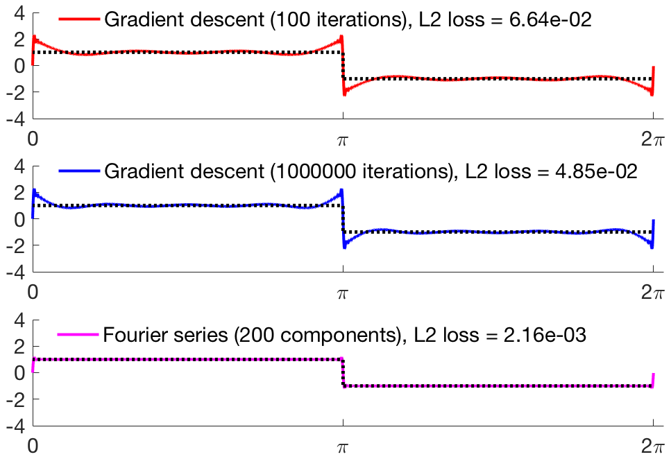
Figure 1: Top: Heaviside step function approximated by $100$ iterations of gradient descent with the Heat kernel (s=0.5). Middle: Approximation after $10^{6}$ iterations of gradient descent. Bottom: Fourier series approximation with $200$ Fourier harmonics.

In contrast, a direct computation of inner products $\langle f,e_{i}\rangle$ yields exact function recovery for any function in $L^{2}([0,2\pi])$ using the amount of computation equivalent to just one step of gradient descent. Thus, we see that the gradient descent is an extremely inefficient way to recover Fourier series for a general periodic function. See Figure 1 for an illustration of this phenomenon. We see that the approximation for the Heaviside function is only marginally improved by going from $100$ to $10^{6}$ iterations of gradient descent. On the other hand, just $200$ Fourier harmonics provide a far more accurate reconstruction.

Things are not much better for functions with more smoothness unless they happen to be extremely smooth with exponential Fourier component decay. Thus in the classification case we expect nearly exponential increase in computational requirements as the margin between classes decreases.

The situation is only mildly improved in dimension $d$, where the span of at most $O^{*}\left(({\log t})^{d/2}\right)$ eigenfunctions of a Gaussian kernel or $O\left(t^{1/p}\right)$ eigenfunctions of an arbitrary $p$-differentiable kernel can be approximated in $t$ iterations. The discussion above shows that the gradient descent with a smooth kernel can be viewed as a heavy regularization of the target function. It is essentially a band-limited approximation with $(\ln t)^{\alpha}$ Fourier harmonics for some $\alpha$. While regularization is often desirable from a generalization/finite sample point of view in machine learning, especially when the number of data points is small, the bias resulting from the application of the gradient descent algorithm cannot be overcome in a realistic number of iterations unless the target functions are extremely smooth or the kernel itself is not infinitely differentiable.

Remark 2.9 (Rate of convergence vs statistical fit).

Note that we can improve convergence by changing the shape parameter of the kernel, i.e. making it more “peaked” (e.g., decreasing the bandwidth $s$ in the definition of the Gaussian kernel) While that does not change the exponential nature of the asymptotics of the eigenvalues, it slows their decay. Unfortunately improved convergence comes at the price of overfitting. In particular, for finite data, using a very narrow Gaussian kernel results in an approximation to the $1$-NN classifier, a suboptimal method which is up to a factor of two inferior to the Bayes optimal classifier in the binary classification case asymptotically. See Appendix H for some empirical results on the bandwidth selection for Gaussian kernels. Another possibility is to use a kernel, such as the Laplace kernel, which is not differentiable at zero. However, it also seems to consistently under-perform more smooth kernels on real data, see Appendix E for some experiments.

Finite sample effects, regularization and early stopping. So far we have discussed the effects of the infinite-data version of gradient descent. We will now discuss issues related to the finite sample setting we encounter in practical machine learning. It is well known (e.g., [B⁺05, RBV10]) that the top eigenvalues of kernel matrices approximate the eigenvalues of the underlying integral operators. Therefore computational obstructions encountered in the infinite case persist whenever the data set is large enough.

Note that for a kernel method, $t$ iterations of gradient descent for $n$ data points require $t\cdot n^{2}$ operations. Thus, gradient descent is computationally pointless unless $t\ll n$. That would allow us to fit only about $O(\log t)$ eigenvectors. In practice we would like to have $t$ to be much smaller than $n$, probably a reasonably small constant.

At this point we should contrast our conclusions with the important analysis of early stopping for gradient descent provided in [YRC07] (see also [RWY14, CARR16]). The authors analyze gradient descent for kernel methods obtaining the optimal number of iterations of the form $t=n^{\theta},\theta\in(0,1)$. That seems to contradict our conclusion that a very large, potentially exponential, number of iterations may be needed to guarantee convergence. The apparent contradiction stems from the assumption in [YRC07] and other works that the regression function $f^{*}$ belongs to the range of some power of the kernel operator $K$. For an infinitely differentiable kernel, that implies super-polynomial spectral decay ($a_{i}=O(\lambda_{i}^{N})$ for any $N>0$). In particular, it implies that $f^{*}$ belongs to any Sobolev space. We do not typically expect such high degree of smoothness in practice, particularly in classification problems. In general, we expect sharp transitions of label probabilities across class boundaries to be typical for many classifications datasets. The Heaviside step function seems to be a simple but reasonable model for that behavior in one dimension. These areas of near-discontinuity will result in slow decay of Fourier coefficients of $f^{*}$ and a mismatch with any infinitely differentiable kernel. Thus a reasonable approximation of $f^{*}$ would require a large number of gradient descent iterations.

Dataset Metric Number of iterations 1 80 1280 10240 81920 MNIST-10k L2 loss train 4.07e-1 9.61e-2 2.60e-2 2.36e-3 2.17e-5 test 4.07e-1 9.74e-2 4.59e-2 3.64e-2 3.55e-2 c-error (test) 38.50% 7.60% 3.26% 2.39% 2.49% HINT-M-10k L2 loss train 8.25e-2 4.58e-2 3.08e-2 1.83e-2 4.21e-3 test 7.98e-2 4.24e-2 3.34e-2 3.14e-2 3.42e-2

To illustrate this point with a real data example, consider the results in the table on the right. We show the results of gradient descent for two subsets of $10000$ points from the MNIST and HINT-M datasets (see Section 6 for the description) respectively. We see that the regression error on the training set is roughly inverse to the number of iterations, i.e. every extra bit of precision requires twice the number of iterations for the previous bit. For comparison, as we are primarily interested in the generalization properties of the solution, we see that the minimum regression ($L^{2}$) error on both test sets is achieved at over $10000$ iterations. This results in at least cubic computational complexity equivalent to that of a direct method. While HINT-M is a regression dataset, the optimal classification accuracy for MNIST is also achieved at about $10000$ iterations.

Regularization “by impatience”/explicit regularization terms. The above discussion suggests that gradient descent applied to kernel methods would typically result in underfitting for most larger datasets. Indeed, even $10000$ iterations of gradient descent is prohibitive when data size is more than $10^{6}$. As we will see in the experimental results section this is indeed the case. SGD ameliorates the problem mildly by allowing us to take approximate steps much faster but even so running standard gradient descent methods to optimality is often impractical. In most cases we observe little need for explicit early stopping rules. Regularization is a result of computational constraints (cf. [YRC07, RWY14, CARR16]) and can be termed regularization “by impatience” as we run out of time/computational budget allotted to the task.

Note that typical forms of regularization, result a large bias along eigenvectors with small eigenvalues $\lambda_{i}$. For example, adding a term of the form $\lambda\|f\|_{\mathcal{K}}$ (Tikhonov regularization/ridge regression) replaces $\frac{1}{\lambda_{i}}$ by $\frac{1}{\lambda+\lambda_{i}}$. While this improves the condition number and hence the speed of convergence, it comes at a high cost in terms of over-regularization/under-fitting as it essentially discards information along eigenvectors with eigenvalues smaller than $\lambda$. In the Fourier series analysis example, introducing $\lambda$ this is similar to considering band-limited functions with $\sim\frac{\sqrt{\log(1/\lambda)}}{s}$ Fourier components. Even for $\lambda=10^{-16}$ (machine precision for double floats) and the kernel parameter $s=1$ we can only fit about $10$ Fourier components! We argue that in most cases there is little need for explicit regularization in the big data regimes as our primary concern is underfitting.

Remark 2.10 (Stochastic gradient descent).

Our discussion so far has been centered entirely on gradient descent. In practice stochastic gradient descent is often used for large data. In our setting, for fixed $\eta$, using SGD results in the same expected step size in each eigendirection as gradient descent. Hence, using SGD does not expand the algorithmic reach of gradient descent, although it speeds up convergence in practice. On the other hand, SGD introduces a number of interesting algorithmic and statistical subtleties. We will address some of them below.

3 EigenPro iteration: extending the reach of gradient descent

We will now propose some practical measures to alleviate the issues related to over-regularization of linear regression by gradient descent. As seen above, one of the key shortcomings of shallow learning methods based on smooth kernels (and their approximations, e.g. Fourier and RBF features) is their fast spectral decay. That observation suggests modifying the corresponding matrix $H$ by decreasing its top eigenvalues. This “partial whitening” enables the algorithm to approximate more target functions in a fixed number of iterations.

It turns out that accurate approximations of the top eigenvectors can be obtained from small subsamples of the data with modest computational expenditure. Moreover, “partially whitened" iteration can be done in a way compatible with stochastic gradient descent thus obviating the need to materialize full covariance/kernel matrices in memory. Combining these observations we construct a low overhead preconditioned Richardson iteration which we call EigenPro iteration.

Preconditioned (stochastic) gradient descent. We will modify the linear system in Eq. 4 with an invertible matrix $P$, called a left preconditioner.

$$PH{\boldsymbol{\alpha}}-P{\boldsymbol{b}}=0$$ (14)

Clearly, the modified system in Eq. 14 and the original system in Eq. 4 have the same solution. The Richardson iteration corresponding to the modified system (preconditioned Richardson iteration) is

$${\boldsymbol{\alpha}}\leftarrow{\boldsymbol{\alpha}}-\eta P(H{\boldsymbol{\alpha}}-{\boldsymbol{b}})$$ (15)

It is easy to see that as long as $\eta\|PH\|<1$ it converges to ${\boldsymbol{\alpha}}^{*}$, the solution of the original linear system.

Preconditioned SGD can be defined similarly by

$${\boldsymbol{\alpha}}\leftarrow{\boldsymbol{\alpha}}-\eta P(H_{m}{\boldsymbol{\alpha}}-{\boldsymbol{b}}_{m})$$ (16)

where we define $H_{m}\mathrel{\overset{\makebox[0.0pt]{\mbox{\tiny def}}}{=}}\frac{2}{m}X_{m}^{T}X_{m}$ and $b_{m}\mathrel{\overset{\makebox[0.0pt]{\mbox{\tiny def}}}{=}}\frac{2}{m}X^{T}_{m}{\boldsymbol{y}}_{m}$ using $(X_{m},{\boldsymbol{y}}_{m})$, a sampled mini-batch of size $m$. This preconditioned iteration also converges to ${\boldsymbol{\alpha}}^{*}$ with properly chosen $\eta$ [Mur98].

Remark 3.1.

Notice that the preconditioned covariance matrix $PH$ does not in general have to be symmetric. It is sometimes convenient to consider the closely related iteration

$${\boldsymbol{\beta}}\leftarrow{\boldsymbol{\beta}}-\eta(P^{\frac{1}{2}}HP^{\frac{1}{2}}{\boldsymbol{\beta}}-P^{\frac{1}{2}}{\boldsymbol{b}})$$ (17)

Here $P^{\frac{1}{2}}HP^{\frac{1}{2}}$ is a symmetric matrix. We see that ${\boldsymbol{\beta}}^{*}=P^{-1/2}{\boldsymbol{\alpha}}^{*}$.

Preconditioning as a linear feature map. It is easy to see that preconditioned iteration in Eq. 17 is in fact equivalent to the standard Richardson iteration in Eq. 5 on a dataset transformed with the linear feature map,

$$\operatorname{\phi}_{P}({\boldsymbol{x}})\mathrel{\overset{\makebox[0.0pt]{\mbox{\tiny def}}}{=}}P^{\frac{1}{2}}{\boldsymbol{x}}$$ (18)

This is a convenient point of view as the transformed data can be stored for future use. It also shows that preconditioning is compatible with most computational methods both in practice and, potentially, in terms of analysis.

3.1 Linear EigenPro

We will now discuss properties desired to make preconditioned GD/SGD methods effective on large scale problems. Thus for the modified iteration in Eq. 15 we would like to choose $P$ to meet the following targets:

Acceleration. The algorithm should provide high accuracy in a small number of iterations.

Initial cost. The preconditioning matrix $P$ should be accurately computable without materializing the full covariance matrix.

Cost per iteration. Preconditioning by $P$ should be efficient per iteration in terms of computation and memory.

0:  $\mathrm{EigenPro}(X,{\boldsymbol{y}},k,m,\eta,\tau,M)$

0:  training data $(X,{\boldsymbol{y}})$, number of eigen-directions $k$, mini-batch size $m$, step size $\eta$, damping factor $\tau$, subsample size $M$

0:  weight of the linear model ${\boldsymbol{\alpha}}$

1:  $[E,\Lambda,\hat{\lambda}_{k+1}]=\mathrm{RSVD}(X,k+1,M)$

2:  $P\mathrel{\overset{\makebox[0.0pt]{\mbox{\tiny def}}}{=}}I-E(I-\tau\hat{\lambda}_{k+1}\Lambda^{-1})E^{T}$

3:  Initialize ${\boldsymbol{\alpha}}\leftarrow 0$

4:  while stopping criteria is False do

5:     $(X_{m},{\boldsymbol{y}}_{m})\leftarrow$ $m$ rows sampled from $(X,{\boldsymbol{y}})$ without replacement

6:     ${\boldsymbol{g}}\leftarrow\frac{1}{m}(X_{m}^{T}(X_{m}{\boldsymbol{\alpha}})-X_{m}^{T}{\boldsymbol{y}}_{m})$

7:     ${\boldsymbol{\alpha}}\leftarrow{\boldsymbol{\alpha}}-\eta P{\boldsymbol{g}}$

8:  end while

Table 1: EigenPro iteration in vector space

The relative approximation error along $i$ the eigenvector for gradient descent after $t$ iterations is $\left(1-\frac{\lambda_{i}(PH)}{\lambda_{1}(PH)}\right)^{t}$. Minimizing the error suggests choosing the preconditioner $P$ to maximize the ratio $\frac{\lambda_{i}(PH)}{\lambda_{1}(PH)}$ for each $i$. We see that modifying the top eigenvalues of $H$ makes the most difference in convergence. For example, decreasing $\lambda_{1}$ improves convergence along all directions, while decreasing any other eigenvalue only speeds up convergence in that direction . However, decreasing $\lambda_{1}$ below $\lambda_{2}$ does not help unless $\lambda_{2}$ is decreased as well. Therefore it is natural to decrease the top $k$ eigenvalues to the maximum amount, i.e. to $\lambda_{k+1}$, leading to the preconditioner

$$\begin{split}P\mathrel{\overset{\makebox[0.0pt]{\mbox{\tiny def}}}{=}}I-\sum_{i=1}^{k}{(1-\frac{\lambda_{k+1}}{\lambda_{i}}){\boldsymbol{e}}_{i}{\boldsymbol{e}}_{i}^{T}}\end{split}$$ (19)

In fact it can be readily seen that $P$ is the optimal preconditioner of the form $I-Q$, where $Q$ is a low rank matrix. We will see that $P$-preconditioned iteration accelerates convergence by approximately a factor of $\lambda_{1}/\lambda_{k}$.

However, exact construction of $P$ involves computing the eigendecomposition of the $d\times d$ matrix $H$, which is not feasible for large data size. To avoid this, we use subsample randomized SVD [HMT11] to obtain an approximate preconditioner, defined as

$$\begin{split}\hat{P}_{\tau}\mathrel{\overset{\makebox[0.0pt]{\mbox{\tiny def}}}{=}}I-\sum_{i=1}^{k}{(1-\tau\frac{\hat{\lambda}_{k+1}}{\hat{\lambda}_{i}})\hat{{\boldsymbol{e}}}_{i}\hat{{\boldsymbol{e}}}_{i}^{T}}\end{split}$$ (20)

where algorithm RSVD (see Appendix A) computes the approximate top eigenvectors $E\leftarrow(\hat{{\boldsymbol{e}}}_{1},\ldots,\hat{{\boldsymbol{e}}}_{k})$ and eigenvalues $\Lambda\leftarrow\textrm{diag}(\hat{\lambda}_{1},\ldots,\hat{\lambda}_{k})$ and $\hat{\lambda}_{k+1}$ for subsample covariance matrix $H_{M}$. Alternatively, a Nyström method based SVD (see Appendix A) can be applied to obtain eigenvectors (slightly less accurate although with little impact on training in practice) through a highly efficient implementation for GPU.

Additionally, we introduce the parameter $\tau$ to counter the effect of approximate top eigenvectors “spilling” into the span of the remaining eigensystem. Using $\tau<1$ is preferable to the obvious alternative of decreasing the step size $\eta$ as it does not decrease the step size in the directions nearly orthogonal to the span of $(\hat{{\boldsymbol{e}}}_{1},\ldots,\hat{{\boldsymbol{e}}}_{k})$. That allows the iteration to converge faster in those directions. In particular, $(\hat{{\boldsymbol{e}}}_{1},\ldots,\hat{{\boldsymbol{e}}}_{k})$ are computed exactly, the step size in other eigendirections will not be affected by the choice of $\tau$.

We call SGD with the preconditioner $\hat{P}_{\tau}$ (Eq. 16) EigenPro iteration. The details of the algorithm are given in Table 1. Moreover, the key step size parameter $\eta$ can be selected in a theoretically sound way discussed below.

3.2 Kernel EigenPro

While EigenPro iteration can be applied to any linear regression problem, it is particularly useful in conjunction with smooth kernels which have fast eigenvalue decay. We will now discuss modifications needed to work directly in the RKHS (primal) setting.

0:  $\mathrm{EigenPro}(\operatorname{k}(\cdot,\cdot),X,{\boldsymbol{y}},k,m,\eta,s_{0})$

0:  kernel function $\operatorname{k}(\cdot,\cdot)$, training data $(X,{\boldsymbol{y}})$, number of eigen-directions $k$, mini-batch size $m$, step size $\eta$, subsample size $M$, damping factor $\tau$

0:  weight of the kernel method ${\boldsymbol{\alpha}}$

1:  $K\mathrel{\overset{\makebox[0.0pt]{\mbox{\tiny def}}}{=}}\operatorname{k}(X,X)$ materialized on demand

2:  $[E,\Lambda,\lambda_{k+1}]\leftarrow\mathrm{RSVD}(K,k+1,M)$

3:  $D\mathrel{\overset{\makebox[0.0pt]{\mbox{\tiny def}}}{=}}E\Lambda^{-1}(I-\tau\lambda_{k+1}\Lambda^{-1})E^{T}$

4:  Initialize ${\boldsymbol{\alpha}}\leftarrow 0$

5:  while stopping criteria is False do

6:     $(K_{m},{\boldsymbol{y}}_{m})\leftarrow$ $m$ rows sampled from $(K,{\boldsymbol{y}})$

7:     ${\boldsymbol{\alpha}}_{m}\mathrel{\overset{\makebox[0.0pt]{\mbox{\tiny def}}}{=}}$ portion of ${\boldsymbol{\alpha}}$ related to $K_{m}$

8:     ${\boldsymbol{g}}_{m}\leftarrow\frac{1}{m}(K_{m}{\boldsymbol{\alpha}}-{\boldsymbol{y}}_{m})$

9:     ${\boldsymbol{\alpha}}_{m}\leftarrow{\boldsymbol{\alpha}}_{m}-\eta{\boldsymbol{g}}_{m}$, ${\boldsymbol{\alpha}}\leftarrow{\boldsymbol{\alpha}}+\eta DK_{m}^{T}{\boldsymbol{g}}_{m}$

10:  end while

Table 2: EigenPro iteration in RKHS space

In this setting, a reproducing kernel $\operatorname{k}(\cdot,\cdot):\mathbb{R}^{N}\times\mathbb{R}^{N}\rightarrow\mathbb{R}$ implies a feature map from $X$ to an RKHS space $\mathcal{H}$ (typically) of infinite dimension. The feature map can be written as $\operatorname{\phi}:x\mapsto k(x,\cdot),\mathbb{R}^{N}\to\mathcal{H}$. This feature map leads to the (shallow) learning problem

$$f^{*}=\arg\min_{f\in\mathcal{H}}\frac{1}{n}\sum_{i=1}^{n}{(\langle f,\operatorname{k}({\boldsymbol{x}}_{i},\cdot)\rangle_{\mathcal{H}}-y_{i})^{2}}$$

Using properties of RKHS, EigenPro iteration in ${\mathcal{H}}$ becomes $f\leftarrow f-\eta\operatorname{P}_{\tau}(\mathcal{K}(f)-\operatorname{b})$ where covariance operator $\mathcal{K}\mathrel{\overset{\makebox[0.0pt]{\mbox{\tiny def}}}{=}}\frac{2}{n}\sum_{i=1}^{n}{\operatorname{k}({\boldsymbol{x}}_{i},\cdot)\otimes\operatorname{k}({\boldsymbol{x}}_{i},\cdot)}$ and $\operatorname{b}\mathrel{\overset{\makebox[0.0pt]{\mbox{\tiny def}}}{=}}\frac{2}{n}\sum_{i=1}^{n}{y_{i}k({\boldsymbol{x}}_{i},\cdot)}$. The top eigensystem of $\mathcal{K}$ forms the preconditioner

$$\operatorname{P}_{\tau}\mathrel{\overset{\makebox[0.0pt]{\mbox{\tiny def}}}{=}}\operatorname{I}-\sum_{i=1}^{k}{(1-\tau\frac{\lambda_{k+1}(\mathcal{K})}{\lambda_{i}(\mathcal{K})})\operatorname{e}_{i}(\mathcal{K})\otimes\operatorname{e}_{i}(\mathcal{K})}$$

Notice that by the Representer theorem [Aro50], $f^{*}$ admits a representation of the form $\sum_{i=1}^{n}{\alpha_{i}\operatorname{k}({\boldsymbol{x}}_{i},\cdot)}$. Parameterizing the above iteration accordingly and applying some linear algebra lead to the following iteration in a finite-dimensional vector space,

$${\boldsymbol{\alpha}}\leftarrow{\boldsymbol{\alpha}}-\eta P_{\tau}(K{\boldsymbol{\alpha}}-{\boldsymbol{y}})$$

where $K\mathrel{\overset{\makebox[0.0pt]{\mbox{\tiny def}}}{=}}[\operatorname{k}({\boldsymbol{x}}_{i},{\boldsymbol{x}}_{j})]_{i,j=1,\ldots,n}$ is the kernel matrix and EigenPro preconditioner $P$ is defined using the top eigensystem of $K$ (assume $K{\boldsymbol{e}}_{i}=\lambda_{i}{\boldsymbol{e}}_{i}$),

$$P_{\tau}\mathrel{\overset{\makebox[0.0pt]{\mbox{\tiny def}}}{=}}I-\sum_{i=1}^{k}{\frac{1}{\lambda_{i}}(1-\tau\frac{\lambda_{k+1}}{\lambda_{i}}){\boldsymbol{e}}_{i}{\boldsymbol{e}}_{i}^{T}}$$

This preconditioner differs from that for the linear case (Eq. 19) with an extra factor of $\frac{1}{\lambda_{i}}$ due to the difference between the parameter space of $\alpha$ and the RKHS space. Table 2 details the SGD version of this iteration.

EigenPro as kernel learning. Another way to view EigenPro is in terms of kernel learning. Assuming that the preconditioner is computed exactly, we see that in the population case EigenPro is equivalent to computing the (distribution-dependent) kernel

$$k_{EP}(x,z)\mathrel{\overset{\makebox[0.0pt]{\mbox{\tiny def}}}{=}}\sum_{i=1}^{k}\lambda_{k+1}e_{i}(x)e_{i}(z)+\sum_{i=k+1}^{\infty}\lambda_{i}e_{i}(x)e_{i}(z)$$

Notice that the RKHS spaces corresponding to $k_{EP}$ and $k$ contain the same functions but have different norms. The norm in $k_{EP}$ is a finite rank modification of the norm in the RKHS corresponding to $k$, a setting reminiscent of [SNB05] where unlabeled data was used to “warp” the norm for semi-supervised learning. However, in our paper the “warping" is purely for computational efficiency.

3.3 Costs and Benefits

We will now discuss the acceleration provided by EigenPro and the overhead associated with the algorithm.

Acceleration. Assuming that the preconditioner $P$ can be computed exactly, EigenPro computes the solution exactly in the span of the top $k+1$ eigenvectors. For $i>k+1$ EigenPro provides the acceleration factor of $\alpha=\frac{\left(1-{\lambda_{i}}/{\lambda_{1}}\right)^{t}}{\left(1-\lambda_{i}/\lambda_{k+1}\right)^{t}}$ along the $i$th eigendirection. Assuming that $\lambda_{i}\ll\lambda_{1}$, a simple calculation shows an acceleration factor of at least $\frac{\lambda_{1}}{\lambda_{k+1}}$ over the standard gradient descent. Note that this assumes full gradient descent and exact computation of the preconditioner. See below for an acceleration analysis in the SGD setting resulting in a potentially somewhat smaller acceleration factor.

Initial cost. To construct the preconditioner $P$, we perform RSVD (Appendix A) to compute the approximate top eigensystem of covariance $H$. Algorithm RSVD has time complexity $O(Md\log{k}+(M+d)k^{2})$ (see [HMT11]). The subsample size $M$ can be much smaller than the data size $n$ while still preserving the accuracy of estimation for top eigenvectors. In addition, we need extra $kd$ memory to store the top-$k$ eigenvectors.

Cost per iteration. For standard SGD with $d$ features (or kernel centers) and mini-batch of size $m$, the computational cost per iteration is $O(md)$. In addition, applying the preconditioner $P$ in EigenPro requires left multiplication by a matrix of rank $k$. That involves $k$ vector-vector dot products for vectors of length $d$, resulting in $k\cdot d$ operations per iteration. Thus EigenPro using top-$k$ eigen-directions needs $O(md+kd)$ operations per iteration. Note that these can be implemented efficiently on a GPU. See Section 6 for actual overhead per iteration achieved in practice.

4 Step Size Selection for EigenPro Preconditioned Methods

We will now discuss the key issue of the step size selection for EigenPro iteration. For iteration involving covariance matrix $H$, $\eta=\left\lVert H\right\rVert^{-1}$ results in optimal (within a factor of $2$) convergence.

This suggests choosing the corresponding step size $\eta=\left\lVert PH\right\rVert^{-1}=\lambda_{k+1}^{-1}$. However, in practice this will lead to divergence due to (1) approximate computation of eigenvectors (2) the randomness inherent in SGD. One possibility would be to compute $\left\lVert PH_{m}\right\rVert$ at every step. That, however, is costly, requiring computing the top singular value for every mini-batch. As the mini-batch can be assumed to be chosen at random, we propose using a lower bound on $\left\lVert H_{m}\right\rVert^{-1}$ (with high probability) as the step size to guarantee convergence at each iteration, which works well in practice.

Linear EigenPro. Consider the EigenPro preconditioned SGD in Eq. 16. For this analysis assume that $P$ is formed by the exact eigenvectors of $H$. Interpreting $P^{\frac{1}{2}}$ as a linear feature map as in Section 2, makes $P^{\frac{1}{2}}H_{m}P^{\frac{1}{2}}$ a random subsample on the dataset $XP^{\frac{1}{2}}$. Now applying Lemma 3 (Appendix C) results in

Theorem 3.

If $\left\lVert{\boldsymbol{x}}\right\rVert^{2}_{2}\leq\kappa$ for any ${\boldsymbol{x}}\in X$ and $\lambda_{k+1}=\lambda_{k+1}(H)$, $\left\lVert PH_{m}\right\rVert$ has following upper bound with probability at least $1-\delta$,

$$\begin{split}\left\lVert PH_{m}\right\rVert\leq\lambda_{k+1}+\frac{2(\lambda_{k+1}+\kappa)}{3m}\ln{\frac{2d}{\delta}}+\sqrt{\frac{2\lambda_{k+1}\kappa}{m}\ln{\frac{2d}{\delta}}}\end{split}$$ (21)

Kernel EigenPro. For EigenPro iteration in RKHS space, we can bound $\left\lVert\operatorname{P}\circ\mathcal{K}_{m}\right\rVert$ with a similar theorem where $\mathcal{K}_{m}$ is the subsample covariance operator and $\operatorname{P}$ is the corresponding EigenPro preconditioner operator. Since $d=dim(\mathcal{K})$ is infinite, we introduce intrinsic dimension from [Tro15] $\mathrm{intdim}(A)\mathrel{\overset{\makebox[0.0pt]{\mbox{\tiny def}}}{=}}\frac{tr(A)}{\left\lVert A\right\rVert}$ where $A:\mathcal{H}\rightarrow\mathcal{H}$ is an arbitrary operator. It can be seen as a measure of the number of dimensions where $A$ has significant spectral content. Let $\mathrm{d}\mathrel{\overset{\makebox[0.0pt]{\mbox{\tiny def}}}{=}}\mathrm{intdim}(\mathbb{E}[(\mathcal{K}_{m}-\mathcal{K})\circ(\mathcal{K}_{m}-\mathcal{K})])$. Then by Lemma 4 (Appendix C), we have

Theorem 4.

If $k({\boldsymbol{x}},{\boldsymbol{x}})\leq\kappa$ for any ${\boldsymbol{x}}\in X$ and $\lambda_{k+1}=\lambda_{k+1}(\mathcal{K})$, with probability at least $1-\delta$ we have,

$$\begin{split}\left\lVert\operatorname{P}\circ\mathcal{K}_{m}\right\rVert\leq\lambda_{k+1}+\frac{2(\lambda_{k+1}+\kappa)}{3m}\ln{\frac{8\mathrm{d}}{\delta}}+\sqrt{\frac{2\lambda_{k+1}\kappa}{m}\ln{\frac{8\mathrm{d}}{\delta}}}\end{split}$$ (22)

Choice of the step size. In both spectral norm bounds Eq. 21 and Eq. 22, $\lambda_{k+1}$ is the dominant term when the mini-batch size $m$ is large. However, in most large-scale settings, $m$ is small, and $\sqrt{\frac{2\lambda_{k+1}\kappa}{m}}$ becomes the dominant term. This suggests choosing step size $\eta\sim\sqrt{\frac{m}{\lambda_{k+1}}}$ leading to acceleration on the order of $\sqrt{\frac{\lambda_{1}}{\lambda_{k+1}}}$ over the standard (unpreconditioned) SGD. That choice works well in practice.

5 EigenPro and Related Work

Recall that the setting of large scale machine learning imposes some fairly specific requirements on the optimization methods. In particular, the computational budget allocated to the problem must not significantly exceed $O(n^{2})$ operations, i.e., a small number of matrix-vector multiplications. That restriction rules out most direct second order methods which require $O(n^{3})$ operations. Approximate second order methods are far more effective computationally. However, they typically rely on low rank matrix approximation, a strategy which underperforms in conjunction with smooth kernels as information along important eigen-directions with small eigenvalues is discarded. Similarly, regularization improves conditioning and convergence but also discards information by biasing small eigen-directions.

While first order methods preserve important information, they, as discussed in this paper, are too slow to converge along eigenvectors with small eigenvalues. It is clear that an effective method must thus be a hybrid approach using approximate second order information in a first order method.

EigenPro is an example of such an approach as the second order information is used in conjunction with an iterative first order method. The things that make EigenPro effective are the following:
1. The second order information (eigenvalues and eigenvectors) is computed efficiently from a subsample of the data. Due to the quadratic loss function, that computation needs to be conducted only once. Moreover, the step size can be fixed throughout the iteration.
2. Preconditioned Richardson iteration is efficient and has a natural stochastic version. Preconditioning by a low rank modification of the identity matrix results in low overhead per iteration. The preconditioned update is computed on the fly without a need to materialize the full preconditioned covariance.
3. EigenPro iteration converges (mathematically) to the same result independently of the preconditioning matrix. That makes EigenPro relatively robust to errors in the second order preconditioning term $P$, in contrast to most approximate second order methods.

We will now discuss some related literature and connections.

First order optimization methods. Gradient based methods, such as gradient descent (GD), stochastic gradient descent (SGD), are classic textbook methods [She94, DJS96, BV04, Bis07]. Recent renaissance of neural networks had drawn significant attention to improving and accelerating these methods, especially, the highly scalable mini-batch SGD. Methods like SAGA [RSB12] and SVRG [JZ13] improve stochastic gradient by periodically evaluated full gradient to achieve variance reduction. Another set of approaches [DHS11, TH12, KB14] compute adaptive step size for each gradient coordinate every iteration. The step size is normally chosen to minimize certain regret bound of the loss function. Most of these methods introduce affordable $O(d)$ computation and memory overhead.

Remark 5.1.

Interpreting EigenPro iteration as a linear “partial whitening" feature map, followed by Richardson iteration, we see that most of these first order methods are compatible with EigenPro. Moreover, many convergence bounds for these methods [BV04, RSB12, JZ13] involve the condition number $\lambda_{1}(H)/\lambda_{d}(H)$. EigenPro iteration generically improves such bounds by (potentially) reducing the condition number to $\lambda_{k+1}(H)/\lambda_{d}(H)$.

Second order/hybrid optimization methods. Second order methods use the inverse of the Hessian matrix or its approximation to accelerate convergence [SYG07, BBG09, MNJ16, BHNS16, ABH16]. A limitations of many of these methods is the need to compute the full gradient instead of the stochastic gradient every iteration [LN89, EM15, ABH16] making them harder to scale to large data.

We note the work [EM15] which analyzed a hybrid first/second order method for general convex optimization with a rescaling term based on the top eigenvectors of the Hessian. That can be viewed as preconditioning the Hessian at every iteration of gradient descent. A related recent work [GOSS16] analyses a hybrid method designed to accelerate SGD convergence for linear regression with ridge regularization. The data are preconditioned by preprocessing (rescaling) all data points along the top singular vectors of the data matrix. The authors provide a detailed analysis of the algorithm depending on the regularization parameter. Another recent second order method PCG [ACW16] accelerates the convergence of conjugate gradient on large kernel ridge regression using a novel preconditioner. The preconditioner is the inverse of an approximate covariance generated with random Fourier features. By controlling the number of random features, this method strikes a balance between preconditioning effect and computational cost. [TRVR16] achieves similar preconditioning effects by solving a linear system involving a subsampled kernel matrix every iteration. While not strictly a preconditioner Nyström with gradient descent(NYTRO) [CARR16] also improves the condition number. Compared to many of these methods EigenPro directly addresses the underlying issues of slow convergence without introducing a bias in directions with small eigenvalues and incurring only a small overhead per iteration both in memory and computation.

Finally, limited memory BFGS (L-BFGS) [LN89] and its variants [SYG07, MNJ16, BHNS16] are among the most effective second order methods for unconstrained nonlinear optimization problems. Unfortunately, they can introduce prohibitive memory and computation overhead for large multi-class problems.

Scalable kernel methods. There is a significant literature on scalable kernel methods including [KSW04, HCL⁺08, SSSSC11, TBRS13, DXH⁺14]. Most of these are first order optimization methods. To avoid the $O(n^{2})$ computation and memory requirement typically involved in constructing the kernel matrix, they often adopt approximations like RBF feature [WS01, QB16, TRVR16] or random Fourier features [RR07, DXH⁺14, TRVR16], which reduces such requirement to $O(nd)$. Exploiting properties of random matrices and the Hadamard transform, [LSS13] further reduces the $O(nd)$ requirement to $O(n\log{d})$ computation and $O(n)$ memory, respectively.

Remark 5.2 (Fourier and other feature maps).

As discussed above, most scalable kernel methods suffer from limited computational reach when used with Gaussian and other smooth kernels. Feature maps, such as Random Fourier Features [RR07], are non-linear transformations and are agnostic with respect to the optimization methods. Still they can be viewed as approximations of smooth kernels and thus suffer from the fast decay of eigenvalues.

Preconditioned linear systems. There is a vast literature on preconditioned linear systems with a number of recent papers focusing on preconditioning kernel matrices, such as for low-rank approximation [FM12, CARR16] and faster convergence [COCF16, ACW16]. In particular, we note [FM12] which suggests approximations using top eigenvectors of the kernel matrix as a preconditioner, an idea closely related to EigenPro.

6 Experimental Results

In this section, we will present a number of experimental results to evaluate EigenPro iteration on a range of datasets.

Name $n$ $d$ Label CIFAR-10 $5\times 10^{4}$ 1024 {0,…,9} MNIST $6\times 10^{4}$ 784 {0,…,9} SVHN $7\times 10^{4}$ 1024 {1,…,10} HINT-S $2\times 10^{5}$ 425 $\{0,1\}^{64}$ TIMIT $1.1\times 10^{6}$ 440 {0,…,143} SUSY $5\times 10^{6}$ 18 $\{0,1\}$ HINT-M $7\times 10^{6}$ 246 $[0,1]^{64}$ MNIST-8M $8\times 10^{6}$ 784 {0,…,9}

Computing Resource. All experiments were run on a single workstation equipped with 128GB main memory, two Intel Xeon(R) E5-2620 processors, and one Nvidia GTX Titan X (Maxwell) GPU.

Datasets. The table on the right summarizes the datasets used in experiments. For image datasets (MNIST [LBBH98], CIFAR-10 [KH09], and SVHN [NWC⁺11]), color images are first transformed to grayscale images. We then rescale the range of each feature to $[0,1]$. For other datasets (HINT-S, HINT-M [HYWW13], TIMIT [GLF⁺93], SUSY [BSW14]), we normalize each feature by z-score. In addition, all multiclass labels are mapped to multiple binary labels.

Metrics. For datasets with multiclass or binary labels, we measure the training result by classification error (c-error), the percentage of predicted labels that are incorrect; for datasets with real valued labels, we adopt the mean squared error (mse).

Kernel methods. For smaller datasets exact solution of kernel regularized least squares (KRLS) gives the error close to optimal for kernel methods with the specific kernel parameters. To handle large dataset, we adopt primal space method, Pegasos [SSSSC11] using the square loss and stochastic gradient. For even larger dataset, we combine SGD and Random Fourier Features [RR07] (RF, see Appendix B) as in [DXH⁺14, TRVR16]. The results of these two methods are presented as the baseline. Then we apply EigenPro to Pegasos and RF as described in Section 3. In addition, we compare the state-of-the-art results of other kernel methods to that of EigenPro in this section.

Hyperparameters. For consistent comparison, all iterative methods use mini-batch of size $m=256$. EigenPro preconditioner is constructed using the top $k=160$ eigenvectors of a subsampled dataset of size $M=4800$. For EigenPro iteration with random features, we set the damping factor $\tau=\frac{1}{4}$. For primal EigenPro $\tau=1$.

Overhead of EigenPro iteration. The right side figure shows that the computational overhead of EigenPro iteration over the standard SGD ranged between $10\%$ and $50\%$. For $k=160$ which is the default setting in all other experiments, EigenPro overhead is approximately $20\%$.

Convergence acceleration by EigenPro for different kernels. Table 3 presents the number of epochs needed by EigenPro and Pegasos to reach the error of the optimal kernel classifier (computed by a direct method on these smaller datasets). The actual error can be found in Appendix E. We see that EigenPro provides acceleration of $6$ to $35$ times in terms of the number of epochs required without any loss of accuracy. The actual acceleration is about $20\%$ less due to the overhead of maintaining and applying a preconditioner.

Table 3: Number of epochs to reach the optimal classification error (by KRLS)

Dataset Size Gaussian Kernel Laplace Kernel Cauchy Kernel EigenPro Pegasos EigenPro Pegasos EigenPro Pegasos MNIST $6\times 10^{4}$ 7 77 4 143 7 78 CIFAR-10 $5\times 10^{4}$ 5 56 13 136 6 107 SVHN $7\times 10^{4}$ 8 54 14 297 17 191 HINT-S $5\times 10^{4}$ 19 164 15 308 13 126

Kernel bandwidth selection. We have investigated the impact of kernel bandwidth selection over convergence and performance for Gaussian kernel. As expected, kernel matrix with smaller bandwidth has slower eigenvalue decay, which in turn accelerates convergence of gradient descent. However, selecting smaller bandwidth also decreases test set performance. When the bandwidth is very small, the Gaussian classifier converges to 1-nearest neighbor method, something which we observe in practice. While 1-NN classifier provides reasonable performance, it has up to twice the error of the optimal Bayes classifier in theory and far from the carefully selected Gaussian kernel classifier in practice. See Appendix H for detailed results.

Comparisons on large datasets. On datasets involving up to a few million points, EigenPro consistently outperforms Pegasos/SGD-RF by a large margin when training with the same number of epochs (Table 4).

Table 4: Error rate after 10 epochs / GPU hours (with Gaussian kernel)

Dataset Size Metric EigenPro Pegasos EigenPro-RF^† SGD-RF^† result hours result hours result hours result hours HINT-S $2\times 10^{5}$ c-error 10.0% 0.1 11.7% 0.1 10.3% 0.2 11.5% 0.1 TIMIT $1\times 10^{6}$ 31.7% 3.2 33.0% 2.2 32.6% 1.5 33.3% 1.0 MNIST-8M $1\times 10^{6}$ 0.8% 3.0 1.1% 2.7 0.8% 0.8 1.0% 0.7 $8\times 10^{6}$ - - 0.7% 7.2 0.8% 6.0 HINT-M $1\times 10^{6}$ mse 2.3e-2 1.9 2.7e-2 1.5 2.4e-2 0.8 2.7e-2 0.6 $7\times 10^{6}$ - - 2.1e-2 5.8 2.4e-2 4.1

$\dagger$ We adopt $D=2\times 10^{5}$ random Fourier features.

Comparisons to the state-of-the-art. In Table 5 we provide a comparison to state-of-the-art results for large datasets recently reported in the kernel literature. All of them use significant computational resources and sometimes complex training procedures. We see that EigenPro improves or matches performance performance on each dataset typically at a small fraction of the computational budget. We notice that the very recent work [MGL⁺17] achieves a better 30.9% error rate on TIMIT (using an AWS cluster). It is not directly comparable to our result as it employs kernel features generated using a new supervised feature selection method. EigenPro can plausibly further improve the training error or decrease computational requirements using this new feature set.

Table 5: Comparison to large scale kernel results (Gaussian kernel)

Dataset Size EigenPro (use 1 GTX Titan X) Reported results error GPU hours epochs source error description MNIST $1\times 10^{6}$ 0.70% 4.8 16 PCG [ACW16] 0.72% 1.1 hours (189 epochs) on 1344 AWS vCPUs $6.7\times 10^{6}$ 0.80%^† 0.8 10 [LML⁺14] 0.85% less than 37.5 hours on 1 Tesla K20m TIMIT $2\times 10^{6}$ 31.7% (32.5%)^‡ 3.2 10 Ensemble [HAS⁺14] 33.5% 512 IBM BlueGene/Q cores BCD [TRVR16] 33.5% 7.5 hours on 1024 AWS vCPUs SUSY $4\times 10^{6}$ 19.8% 0.1 0.6 Hierarchical [CAS16] $\approx 20\%$ 0.6 hours on IBM POWER8

$\dagger$ This result is produced by EigenPro-RF using $1\times 10^{6}$ data points. • $\ddagger$ Our TIMIT training set ($1\times 10^{6}$ data points) was generated following a standard practice in the speech community [PGB⁺11] by taking 10ms frames and dropping the glottal stop ’q’ labeled frames in core test set ($1.2\%$ of total test set). [HAS⁺14] adopts 5ms frames, resulting in $2\times 10^{6}$ data points, and keeping the glottal stop ’q’. Taking the worst case scenario for our setting, if we mislabel all glottal stops, the corresponding frame-level error will increase from $31.7\%$ to $32.5\%$.

7 Conclusion and perspective

In this paper we have considered a subtle trade-off between smoothness and computation for gradient-descent based method. While smooth output functions, such as those produced by kernel algorithms with smooth kernels, are often desirable and help generalization (as, for example, encoded in the notion of algorithmic stability [BE02]) there appears to be a hidden but very significant computational cost when the smoothness of the kernel is mismatched with that of the target function. We argue and provide experimental evidence that these mismatches are common in standard classification problems. In particular, we view effectiveness of EigenPro as another piece of supporting evidence.

An important direction of future work is to understand whether this is a universal phenomenon encompassing a range of learning methods or something pertaining to the kernel setting. Specifically, the implications of this idea for deep neural networks need to be explored. Indeed, there is a body of evidence indicating that training neural networks results in highly non-smooth functions. For one thing, they can easily fit data even when the labels are randomly assigned [ZBH⁺16]. Moreover, the pervasiveness of adversarial [SZS⁺13] and even universal adversarial examples common to different networks [MDFFF16] suggests that there are many directions non-smoothness in the neighborhood of nearly any data point. Why neural networks show generalization despite this evident non-smoothness, remains a key open question.

Finally, we have seen that training of kernel methods on large data can be significantly improved by simple algorithmic modifications of first order iterative algorithms using limited second order information. It appears that purely second order methods cannot provide major improvements as low-rank approximations needed for dealing large data discard information corresponding to the higher frequency components present in the data. Better understanding of the computational and statistical issues and the trade-offs inherent in training, would no doubt result in even better shallow algorithms making them more competitive with deep networks on a given computational budget.

Appendix A Scalable truncated SVD

.95

0:  $\mathrm{RSVD}(X,k,M)$, adapted from [HMT11]

0:  $n\times d$ matrix $X$, number of eigen-directions $k$, subsample size $M$

0:  $({\boldsymbol{e}}_{1}(H_{M}),\ldots,{\boldsymbol{e}}_{k}(H_{M}))$, $\mathrm{diag}(\lambda_{1}(H_{M}),\ldots,\lambda_{k}(H_{M})),\lambda_{k+1}(H_{M})$

1:  $X_{M}\leftarrow$ $M$ rows sampled from $X$ without replacement

2:  $[\lambda_{1}(X_{M}),\ldots,\lambda_{k+1}(X_{M})]$, $[{\boldsymbol{v}}_{1}(X_{M}),\ldots,{\boldsymbol{v}}_{k}(X_{M})]$ $\leftarrow\mathrm{rsvd}(X_{M},k+1)$, non-Hermitian version of Algorithm 5.6 in [HMT11] (${\boldsymbol{v}}_{i}(X)\mathrel{\overset{\makebox[0.0pt]{\mbox{\tiny def}}}{=}}$ $i$-th right singular vector)

3:  $\lambda_{i}(H_{M})\leftarrow\sqrt{\frac{n}{M}}\lambda_{i}(X_{M})$, ${\boldsymbol{e}}_{i}(H_{M})\leftarrow{\boldsymbol{v}}_{i}(X_{M})$ for $i=1,\ldots,k$

.95

0:  $\mathrm{NSVD}(X,k,M)$, adapted from [WS01]

0:  $n\times d$ matrix $X$, number of eigen-directions $k$, subsample size $M$

0:  $({\boldsymbol{e}}_{1}(H_{M}),\ldots,{\boldsymbol{e}}_{k}(H_{M}))$, $\mathrm{diag}(\lambda_{1}(H_{M}),\ldots,\lambda_{k}(H_{M})),\lambda_{k+1}(H_{M})$

1:  $X_{M}\leftarrow$ $M$ rows sampled from $X$ without replacement

2:  $W\leftarrow\frac{n}{M}X_{M}X_{M}^{T}$

3:  $[\lambda_{1}(W),\ldots,\lambda_{k+1}(W)]$, $[{\boldsymbol{v}}_{1}(W),\ldots,{\boldsymbol{v}}_{k}(W)]$ $\leftarrow\mathrm{svd}(W,k+1)$

4:  $\lambda_{i}(H_{M})\leftarrow\lambda_{i}(W)$, $\tilde{{\boldsymbol{e}}}_{i}\leftarrow\frac{n}{M}X_{M}^{T}{\boldsymbol{v}}_{i}(W)$ for $i=1,\ldots,k$

5:  $({\boldsymbol{e}}_{1}(H_{M}),\ldots,{\boldsymbol{e}}_{k}(H_{M}))\leftarrow$ $\mathrm{orthogonalize}(\tilde{{\boldsymbol{e}}}_{1},\ldots,\tilde{{\boldsymbol{e}}}_{k})$

Given data matrix $X$, Algorithm RSVD computes its approximate top eigensystem using corresponding subsample covariance matrix $H_{M}\mathrel{\overset{\makebox[0.0pt]{\mbox{\tiny def}}}{=}}\frac{1}{M}X_{M}^{T}X_{M}$. The algorithm has time complexity $O(Md\log{k}+(M+d)k^{2})$ according to [HMT11].

The selection of subsample size $M$ depends on the eigenvalue decay rate of the covariance. Specifically, we choose $M=4800$, which is much smaller than the size of training sets in our experiments. Thus, when $k=160$, RSVD only takes a few minuets computation to complete even that the data (or kernel matrix) dimension $d$ exceeds $10^{6}$.

When computing the approximate top-eigensystem of the covariance for the EigenPro preconditioner, Nyström method based SVD (NSVD) is an alternative method with theoretical time complexity $O(Mdk+M^{3})$ worse than that of RSVD. However, its GPU implementation often outrun the corresponding RSVD implementation (due to applying SVD upon an $M\times M$ matrix instead of an $M\times d$ matrix). In practice, NSVD is able to obtain the approximate top-160 eigensystem of a kernel matrix with dimension $7\cdot 10^{6}$ in less than 2.5 minuets using a single GTX Titan X (Maxwell).

Note that the results returned by NSVD normally involve larger approximation error than that by RSVD (using the same $M$). While in our experiments, this increase of the approximation error has negligible impact on the final regression/classification performance, as well as the convergence rate.

Appendix B Kernel-related feature maps

Random Fourier features (RFF) [RR07]. The random Fourier feature map $\mathbb{R^{N}}\to\mathbb{R^{d}}$ is defined by

$$\operatorname{\phi}_{\mathrm{rff}}({\boldsymbol{x}})\mathrel{\overset{\makebox[0.0pt]{\mbox{\tiny def}}}{=}}\sqrt{2d^{-1}}(\cos({\boldsymbol{\omega}}_{1}^{T}{\boldsymbol{x}}+b_{1}),\ldots,\cos({\boldsymbol{\omega}}_{d}^{T}{\boldsymbol{x}}+b_{d}))^{T}$$

Here ${\boldsymbol{\omega}}_{1},\dots,{\boldsymbol{\omega}}_{d}$ are sampled from the distribution $\frac{1}{2\pi}\int{\exp(-j{\boldsymbol{\omega}}^{T}\delta)\operatorname{k}(\delta)}{d\Delta}$ and $b_{1},\ldots,b_{d}$ from uniform distribution on $[0,2\pi]$. It can be shown that the inner product in the feature space approximates a Gaussian kernel $\operatorname{k}(\cdot,\cdot)$, i.e., $\lim_{D\rightarrow\infty}{\operatorname{\phi}_{\mathrm{rff}}({\boldsymbol{x}})^{T}\operatorname{\phi}_{\mathrm{rff}}({\boldsymbol{y}})}=\operatorname{k}({\boldsymbol{x}},{\boldsymbol{y}})$.

Radial basis function network (RBF) features.This setting involves feature map related to kernel $\operatorname{k}(\cdot,\cdot)$, defined as

$$\operatorname{\phi}_{\mathrm{rbf}}({\boldsymbol{x}})\mathrel{\overset{\makebox[0.0pt]{\mbox{\tiny def}}}{=}}(\operatorname{k}({\boldsymbol{x}},{\boldsymbol{z}}_{1}),\dots,\operatorname{k}({\boldsymbol{x}},{\boldsymbol{z}}_{d}))^{T}$$

where $\{z_{i}\}_{i=1}^{d}$are network centers. Note there are various strategies for selecting centers, e.g., randomly sampling from $X$ [CARR16] or by computing K-means centers leading to different interpretations in terms of data-dependent kernels [QB16].

Appendix C Concentration bounds

Spectral norm of subsample covariance matrix. With subsample size $m$, $H_{m}\mathrel{\overset{\makebox[0.0pt]{\mbox{\tiny def}}}{=}}\frac{1}{m}X_{m}^{T}X_{m}$ is the subsample covariance matrix corresponding to covariance $H$ defined in Eq. 3. To bound its approximation error, $\left\lVert H_{m}-H\right\rVert$, we need the following concentration theorem,

Theorem (Matrix Bernstein [Tro15]).

Let $S_{1},\ldots,S_{m}$ be independent random Hermitian matrices with dimension $d\times d$. Assume that each matrix satisfies

$$\mathbb{E}[S_{i}]=0\leavevmode\nobreak\ \leavevmode\nobreak\ \mathit{and}\leavevmode\nobreak\ \leavevmode\nobreak\ \left\lVert S_{i}\right\rVert\leq L\leavevmode\nobreak\ \leavevmode\nobreak\ \mathit{for}\leavevmode\nobreak\ i=1,\ldots,m$$ (23)

Then for any $t>0$, random matrix $Z\mathrel{\overset{\makebox[0.0pt]{\mbox{\tiny def}}}{=}}\sum_{i=1}^{m}{S_{i}}$ has bound

$$P\{\left\lVert Z\right\rVert\geq t\}\leq 2d\cdot\exp{\left(\frac{-t^{2}/2}{v(Z)+Lt/3}\right)}$$ (24)

where $v(Z)\mathrel{\overset{\makebox[0.0pt]{\mbox{\tiny def}}}{=}}\left\lVert\mathbb{E}[Z^{T}Z]\right\rVert$.

Applying Matrix Bernstein theorem to the subsample covariance $H_{m}$ leads to the following Lemma,

Lemma 1.

If $\left\lVert{\boldsymbol{x}}\right\rVert^{2}_{2}\leq\kappa$ for any ${\boldsymbol{x}}\in X$ and $\lambda_{1}=\left\lVert H\right\rVert$, $\left\lVert H_{m}-H\right\rVert$ has following upper bound with probability at least $1-\delta$,

$$\begin{split}\left\lVert H_{m}-H\right\rVert&\leq\sqrt{\left(\frac{\lambda_{1}+\kappa}{3m}\ln{\frac{2d}{\delta}}\right)^{2}+\frac{2\lambda_{1}\kappa}{m}\ln{\frac{2d}{\delta}}}+\frac{\lambda_{1}+\kappa}{3m}\ln{\frac{2d}{\delta}}\end{split}$$ (25)

Proof.

Consider subsample covariance matrix $H_{m}=\frac{1}{m}\sum_{i=1}^{m}{{\boldsymbol{x}}_{i}{\boldsymbol{x}}_{i}^{T}}$ using ${\boldsymbol{x}}_{1},\ldots,{\boldsymbol{x}}_{m}$ randomly sampled from dataset $X$. For each sampled point ${\boldsymbol{x}}_{i},\ldots,{\boldsymbol{x}}_{m}$, let

$$S_{i}\mathrel{\overset{\makebox[0.0pt]{\mbox{\tiny def}}}{=}}\frac{1}{m}({\boldsymbol{x}}_{i}{\boldsymbol{x}}_{i}^{T}-H)$$ (26)

Clearly, $S_{1},\ldots,S_{m}$ are independent random Hermitian matrices. Since $\mathbb{E}[{\boldsymbol{x}}_{i}{\boldsymbol{x}}_{i}^{T}]=\mathbb{E}[H_{m}]=H$ and $\left\lVert{\boldsymbol{x}}_{i}\right\rVert_{2}^{2}\leq\kappa$ for $i=1,\ldots,m$, we have

$$\mathbb{E}[S_{i}]=0\leavevmode\nobreak\ \mathit{and}\leavevmode\nobreak\ \left\lVert S_{i}\right\rVert\leq\frac{\lambda_{1}+\kappa}{m}\leavevmode\nobreak\ \leavevmode\nobreak\ for\leavevmode\nobreak\ i=1,\ldots,m$$ (27)

Furthermore, notice that for any $i=1,\ldots,m$, we have

$$\begin{split}\mathbb{E}[S_{i}^{2}]&=\frac{1}{m^{2}}\mathbb{E}[{\boldsymbol{x}}_{i}{\boldsymbol{x}}_{i}^{T}{\boldsymbol{x}}_{i}{\boldsymbol{x}}_{i}^{T}-{\boldsymbol{x}}_{i}{\boldsymbol{x}}_{i}^{T}H-H{\boldsymbol{x}}_{i}{\boldsymbol{x}}_{i}^{T}+H^{2}]\\ &=\frac{1}{m^{2}}(\mathbb{E}[\left\lVert{\boldsymbol{x}}_{i}\right\rVert^{2}{\boldsymbol{x}}_{i}{\boldsymbol{x}}_{i}^{T}])-H^{2})\\ &\preceq\frac{1}{m^{2}}(\kappa H-H^{2})\preceq\frac{\kappa}{m^{2}}H\end{split}$$ (28)

Hence the spectral norm has the following upper bound,

$$\left\lVert\mathbb{E}[S_{i}^{2}]\right\rVert\leq\frac{\lambda_{1}\kappa}{m^{2}}$$ (29)

The sum of the random matrices, $H_{m}-H=\sum_{i=1}^{m}{S_{i}}$, can be bounded as follows:

$$\begin{split}v(H_{m}-H)&=\left\lVert\mathbb{E}[(H_{m}-H)^{T}(H_{m}-H)]\right\rVert\\ &=\left\lVert\sum_{i=1}^{m}{\mathbb{E}[S_{i}^{2}]}\right\rVert\leq\sum_{i=1}^{m}{\left\lVert\mathbb{E}[S_{i}^{2}]\right\rVert}\leq\frac{\lambda_{1}\kappa}{m}\end{split}$$ (30)

Now applying Matrix Bernstein Theorem yields

$$\begin{split}P\{\left\lVert H_{m}-H\right\rVert\geq t\}\leq 2d\cdot\exp{\left(\frac{-t^{2}/2}{v(H_{m}-H)+\frac{(\lambda_{1}+\kappa)t}{3m}}\right)}\end{split}$$ (31)

Let the right side of Eq. 31 be $\delta$, we obtain that

$$\begin{split}t&=\sqrt{\left(\frac{\lambda_{1}+\kappa}{3m}\ln{\frac{2d}{\delta}}\right)^{2}+\frac{2\lambda_{1}\kappa}{m}\ln{\frac{2d}{\delta}}}+\frac{\lambda_{1}+\kappa}{3m}\ln{\frac{2d}{\delta}}\end{split}$$ (32)

Therefore, with probability at least $1-\delta$, we have

$$\left\lVert H_{m}-H\right\rVert\leq t$$ (33)

∎

Spectral norm of subsample covariance operator. For EigenPro iteration in RKHS, its step size selection is related to covariance operator $\mathcal{K}$ defined in Eq. 13. Similarly, under the SGD setting, we need to bound $\left\lVert\mathcal{K}_{m}-\mathcal{K}\right\rVert$ where $\mathcal{K}_{m}f(x)\mathrel{\overset{\makebox[0.0pt]{\mbox{\tiny def}}}{=}}\frac{1}{m}\sum_{i=1}^{m}{k(x,x_{i})f(x_{i})}$ is the corresponding subsample covariance operator. Thus we introduce the following Bernstein inequality for random operators. This inequality differs from its vector space version (Matrix Bernstein) by replacing the space dimension with the intrinsic dimension, defined as

$$\mathrm{d}(V)\mathrel{\overset{\makebox[0.0pt]{\mbox{\tiny def}}}{=}}\frac{tr(\operatorname{V})}{\left\lVert\operatorname{V}\right\rVert}$$ (34)

Theorem (Operator Bernstein, adapted from [Min17, Tro15]).

Let $S_{i}:\mathcal{H}\rightarrow\mathcal{H},i=1,\ldots,m$ be independent random Hermitian operators. Assume that each operator satisfies

$$\mathbb{E}[S_{i}]=0\leavevmode\nobreak\ \leavevmode\nobreak\ \mathit{and}\leavevmode\nobreak\ \leavevmode\nobreak\ \left\lVert S_{i}\right\rVert\leq L\leavevmode\nobreak\ \leavevmode\nobreak\ \mathit{for}\leavevmode\nobreak\ i=1,\ldots,m$$ (35)

Consider random Hermitian operator $\operatorname{Z}\mathrel{\overset{\makebox[0.0pt]{\mbox{\tiny def}}}{=}}\sum_{i=1}^{m}{S_{i}}$. Its variance $V\mathrel{\overset{\makebox[0.0pt]{\mbox{\tiny def}}}{=}}\mathbb{E}[\operatorname{Z}^{2}]$ is also an operator on $\mathcal{H}$. For convenience, let the intrinsic dimension (Eq. 34) and the spectral norm of the variance operator be

$$\mathrm{d}\mathrel{\overset{\makebox[0.0pt]{\mbox{\tiny def}}}{=}}\mathrm{d}(V)\leavevmode\nobreak\ \leavevmode\nobreak\ \mathit{and}\leavevmode\nobreak\ \leavevmode\nobreak\ v\mathrel{\overset{\makebox[0.0pt]{\mbox{\tiny def}}}{=}}\left\lVert V\right\rVert$$

Then for any $t\geq\sqrt{v}+L/3$, we have

$$P\{\left\lVert\operatorname{Z}\right\rVert\geq t\}\leq 8\mathrm{d}\cdot\exp{\left(\frac{-t^{2}/2}{v+Lt/3}\right)}$$ (36)

This theorem can be applied to bound $\left\lVert\mathcal{K}_{m}-\mathcal{K}\right\rVert$,

Lemma 2.

If $k({\boldsymbol{x}},{\boldsymbol{x}})\leq\kappa$ for any ${\boldsymbol{x}}\in X$ and $\lambda_{1}=\left\lVert\mathcal{K}\right\rVert$, $\left\lVert\mathcal{K}_{m}-\mathcal{K}\right\rVert$ has following upper bound with probability at least $1-\delta$,

$$\begin{split}\left\lVert\mathcal{K}_{m}-\mathcal{K}\right\rVert&\leq\sqrt{\left(\frac{\lambda_{1}+\kappa}{3m}\ln{\frac{8\mathrm{d}}{\delta}}\right)^{2}+\frac{2\lambda_{1}\kappa}{m}\ln{\frac{8\mathrm{d}}{\delta}}}+\frac{\lambda_{1}+\kappa}{3m}\ln{\frac{8\mathrm{d}}{\delta}}\end{split}$$ (37)

Proof.

Consider subsample covariance operator $\mathcal{K}_{m}f({\boldsymbol{x}})\mathrel{\overset{\makebox[0.0pt]{\mbox{\tiny def}}}{=}}\frac{1}{m}\sum_{i=1}^{m}{k({\boldsymbol{x}},{\boldsymbol{x}}_{i})f({\boldsymbol{x}}_{i})}$ defined by ${\boldsymbol{x}}_{1},\ldots,{\boldsymbol{x}}_{m}$ randomly sampled from dataset $X$. For each sampled point ${\boldsymbol{x}}_{i},\ldots,{\boldsymbol{x}}_{m}$, let

$$\operatorname{S}_{i}f({\boldsymbol{x}})\mathrel{\overset{\makebox[0.0pt]{\mbox{\tiny def}}}{=}}\frac{1}{m}(k({\boldsymbol{x}},{\boldsymbol{x}}_{i})f({\boldsymbol{x}}_{i})-\mathcal{K}f({\boldsymbol{x}}))$$ (38)

Clearly, $\operatorname{S}_{1},\ldots,\operatorname{S}_{m}$ are independent random Hermitian operators. Since $\mathbb{E}[k({\boldsymbol{x}},{\boldsymbol{x}}_{i})f({\boldsymbol{x}}_{i})]=\mathcal{K}f({\boldsymbol{x}})$ and $\left\lVert k(x_{i},\cdot)\right\rVert_{\mathcal{H}}=k({\boldsymbol{x}}_{i},{\boldsymbol{x}}_{i})\leq\kappa$ for $i=1,\ldots,m$, we have

$$\mathbb{E}[\operatorname{S}_{i}]=0\leavevmode\nobreak\ \mathit{and}\leavevmode\nobreak\ \left\lVert\operatorname{S}_{i}\right\rVert\leq\frac{\lambda_{1}+\kappa}{m}\leavevmode\nobreak\ \leavevmode\nobreak\ for\leavevmode\nobreak\ i=1,\ldots,m$$ (39)

Furthermore, for any $f\in\mathcal{H}$, the variance operator of $\operatorname{S}_{i}$ equals

$$\begin{split}\mathbb{E}[\operatorname{S}_{i}^{2}]f({\boldsymbol{x}})&=\frac{1}{m^{2}}(\mathbb{E}[k({\boldsymbol{x}}_{i},{\boldsymbol{x}}_{i})k({\boldsymbol{x}},{\boldsymbol{x}}_{i})f({\boldsymbol{x}}_{i})]-\mathcal{K}^{2}f({\boldsymbol{x}}))\\ &=\frac{1}{m^{2}}(k({\boldsymbol{x}}_{i},{\boldsymbol{x}}_{i})\mathcal{K}f({\boldsymbol{x}})-\mathcal{K}^{2}f({\boldsymbol{x}}))\end{split}$$ (40)

As $k({\boldsymbol{x}}_{i},{\boldsymbol{x}}_{i})\leq\kappa$ and $\mathcal{K}$ is positive semi-definite, this variance operator is bounded by

$$\mathbb{E}[\operatorname{S}_{i}^{2}]\preceq\frac{1}{m^{2}}(\kappa\mathcal{K}-\mathcal{K}^{2})\preceq\frac{\kappa}{m^{2}}\mathcal{K}$$

Hence its spectral norm has upper bound,

$$\left\lVert\mathbb{E}[\operatorname{S}_{i}^{2}]\right\rVert\leq\frac{\lambda_{1}\kappa}{m^{2}}$$ (41)

Since $\operatorname{S}_{i}$ and $\operatorname{S}_{j}$ are independent for $i\neq j$, $\mathbb{E}[\operatorname{S}_{i}\operatorname{S}_{j}]f(x)\equiv 0$ almost everywhere. Then the sum of the random operators, $\mathcal{K}_{m}-\mathcal{K}=\sum_{i=1}^{m}{\operatorname{S}_{i}}$, can be bounded as follows:

$$\begin{split}v(\mathcal{K}_{m}-\mathcal{K})&=\left\lVert\sum_{i=1}^{m}{\mathbb{E}[\operatorname{S}_{i}^{2}]}\right\rVert\leq\sum_{i=1}^{m}{\left\lVert\mathbb{E}[\operatorname{S}_{i}^{2}]\right\rVert}\leq\frac{\lambda_{1}\kappa}{m}\end{split}$$ (42)

Now we can apply the Operator Bernstein on $\mathcal{K}_{m}-\mathcal{K}$ which yields concentration bound,

$$\begin{split}P\{\left\lVert\mathcal{K}_{m}-\mathcal{K}\right\rVert\geq t\}\leq 8\mathrm{d}\cdot\exp{\left(\frac{-t^{2}/2}{v(\mathcal{K}_{m}-\mathcal{K})+\frac{(\lambda_{1}+\kappa)t}{3m}}\right)}\end{split}$$ (43)

for any $t\geq\sqrt{v(\mathcal{K}_{m}-\mathcal{K})}+\frac{(\lambda_{1}+\kappa)}{3m}$. Let the right side of Eq. 43 be $\delta$, we obtain that

$$\begin{split}t&=\sqrt{\left(\frac{\lambda_{1}+\kappa}{3m}\ln{\frac{8\mathrm{d}}{\delta}}\right)^{2}+\frac{2\lambda_{1}\kappa}{m}\ln{\frac{8\mathrm{d}}{\delta}}}+\frac{\lambda_{1}+\kappa}{3m}\ln{\frac{8\mathrm{d}}{\delta}}\end{split}$$ (44)

Therefore, for any $\delta\leq 8\mathrm{d}\cdot e$, with probability at least $1-\delta$, we have

$$\left\lVert\mathcal{K}_{m}-\mathcal{K}\right\rVert\leq t$$ (45)

According to the definition of the intrinsic dimension, $\mathrm{d}\geq 1$. Thus $\delta\leq 8\mathrm{d}\cdot e$ is true for any $\delta\in[0,1]$. ∎

Upper bound on the spectral norm of subsample covariance. Applying Lemma 1 to $\left\lVert H_{m}-H\right\rVert$ and using the inequality $\left\lVert H_{m}\right\rVert\leq\left\lVert H\right\rVert+\left\lVert H_{m}-H\right\rVert$, one can obtain the following

Lemma 3.

If $\left\lVert{\boldsymbol{x}}\right\rVert^{2}_{2}\leq\kappa$ for any ${\boldsymbol{x}}\in X$, then with probability at least $1-\delta$,

$$\begin{split}\left\lVert H_{m}\right\rVert\leq\lambda_{1}+\frac{2(\lambda_{1}+\kappa)}{3m}\ln{\frac{2d}{\delta}}+\sqrt{\frac{2\lambda_{1}\kappa}{m}\ln{\frac{2d}{\delta}}}\end{split}$$ (46)

Similarly, we can bound the spectral norm of the subsample covariance operator $\mathcal{K}_{m}$ by using Lemma 2.

Lemma 4.

If $k({\boldsymbol{x}},{\boldsymbol{x}})\leq\kappa$ for any ${\boldsymbol{x}}\in X$, then with probability at least $1-\delta$,

$$\begin{split}\left\lVert\mathcal{K}_{m}\right\rVert\leq\lambda_{1}+\frac{2(\lambda_{1}+\kappa)}{3m}\ln{\frac{8\mathrm{d}}{\delta}}+\sqrt{\frac{2\lambda_{1}\kappa}{m}\ln{\frac{8\mathrm{d}}{\delta}}}\end{split}$$ (47)

Appendix D $\left\lVert{\boldsymbol{\alpha}}\right\rVert_{2}$  during the training of (primal) kernel method

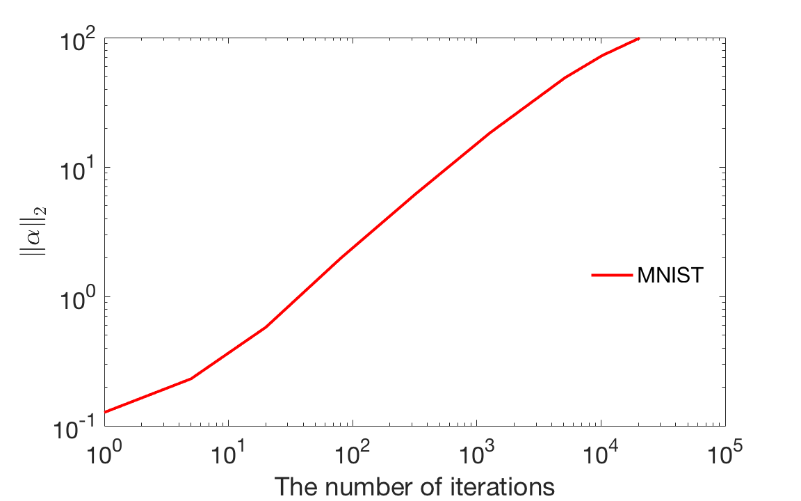
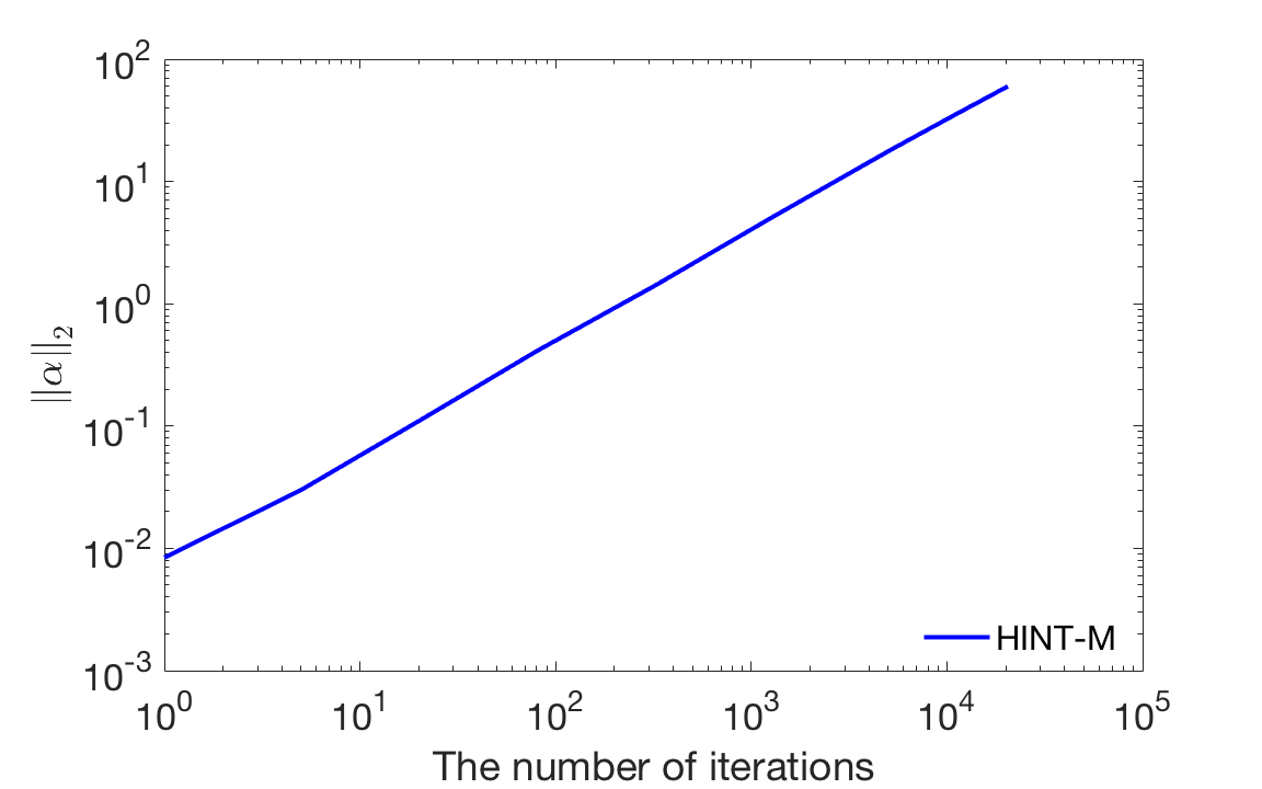
Figure 2: Change of $\left\lVert\alpha\right\rVert_{2}$ during graident descent training (Pegasos) on subsample datasets (10000 points)

Here ${\boldsymbol{\alpha}}=(\alpha_{1},\ldots,\alpha_{n})^{T}$ is the representation of the solution $f$ under basis $\{k({\boldsymbol{x}}_{i},\cdot)\}_{i=1}^{n}$ such that $f=\sum_{i=1}^{n}{\alpha_{i}k({\boldsymbol{x}}_{i},\cdot)}$. Therefore, $\left\lVert{\boldsymbol{\alpha}}\right\rVert_{2}=\left\lVert f\right\rVert_{L^{2}}$.

Appendix E Kernel selection

Best classification error (for KRLS)

Dataset	Size	Gaussian	Laplace	Cauchy
MNIST	$6\times 10^{4}$	1.3%	1.6%	1.5%
CIFAR-10	$5\times 10^{4}$	49.5%	48.9%	48.4%
SVHN	$7\times 10^{4}$	18.0%	18.5%	18.0%
HINT-S	$5\times 10^{4}$	11.3%	11.4%	11.3%

The table on the right side compares optimal performance for three different kernels: the Gaussian kernel $k_{1}(x,y)\mathrel{\overset{\makebox[0.0pt]{\mbox{\tiny def}}}{=}}\exp(-\frac{\left\lVert x-y\right\rVert^{2}}{2\sigma^{2}})$, the Laplace kernel $k_{2}(x,y)\mathrel{\overset{\makebox[0.0pt]{\mbox{\tiny def}}}{=}}\exp(-\frac{\left\lVert x-y\right\rVert}{\sigma})$, and the Cauchy kernel $k_{3}(x,y)\mathrel{\overset{\makebox[0.0pt]{\mbox{\tiny def}}}{=}}(1+\frac{\left\lVert x-y\right\rVert^{2}}{\sigma^{2}})^{-1}$. With bandwidth $\sigma$ selected by cross validation, the performance of the Gaussian kernel is generally comparable to that of the Cauchy kernel. The Laplace kernel performs worst possibly due to its non-smoothness.

Table 6: Classification error on MNIST with different kernels

$N_{Epoch}$ Gaussian Kernel ($\sigma^{2}=25$) Laplace Kernel ($\sigma=10$) Cauchy Kernel ($\sigma^{2}=40$) EigenPro Pegasos EigenPro Pegasos EigenPro Pegasos train test train test train test train test train test train test 1 0.92% 2.03% 5.12% 5.21% 0.16% 2.06% 7.39% 7.21% 0.41% 1.91% 6.05% 5.96% 5 0.10% 1.44% 2.36% 2.84% 0.0% 1.62% 3.42% 4.26% 0.0% 1.31% 2.76% 3.44% 10 0.01% 1.23% 1.58% 2.32% 0.0% 1.58% 2.18% 3.39% 0.0% 1.32% 1.76% 2.57% 20 0.0% 1.20% 0.90% 1.93% 0.0% 1.57% 1.09% 2.57% 0.0% 1.30% 0.91% 2.12% 40 0.0% 1.20% 0.39% 1.65% 0.0% 1.57% 0.32% 2.14% 0.0% 1.30% 0.30% 1.78% 80 0.0% 1.23% 0.14% 1.41% 0.0% 1.57% 0.03% 1.85% 0.0% 1.29% 0.06% 1.56% 160 0.0% 1.21% 0.03% 1.24% 0.0% 1.57% 0.0% 1.71% 0.0% 1.29% 0.01% 1.36%

Table 7: L2 loss on MNIST with different kernels

$N_{Epoch}$ Gaussian Kernel ($\sigma^{2}=25$) Laplace Kernel ($\sigma=10$) Cauchy Kernel ($\sigma^{2}=40$) EigenPro Pegasos EigenPro Pegasos EigenPro Pegasos train test train test train test train test train test train test 1 2.4e-2 3.2e-2 6.9e-2 6.8e-2 2.4e-2 3.5e-2 9.4e-2 9.3e-2 1.8e-2 3.0e-2 7.9e-2 7.8e-2 5 8.6e-3 2.4e-2 4.0e-2 4.3e-2 1.7e-3 2.5e-2 5.3e-2 5.6e-2 3.0e-3 2.2e-2 4.4e-2 4.7e-2 10 4.3e-3 2.2e-2 3.1e-2 3.6e-2 1.0e-4 2.4e-2 4.0e-2 4.6e-2 8.0e-4 2.1e-2 3.3e-2 3.9e-2 20 1.8e-3 2.1e-2 2.3e-2 3.1e-2 0 2.4e-2 2.8e-2 3.9e-2 1.0e-4 2.0e-2 2.3e-2 3.2e-2 40 6.1e-4 2.1e-2 1.6e-2 2.7e-2 0 2.4e-2 1.7e-2 3.2e-2 0 2.0e-2 1.5e-2 2.7e-2 80 2.2e-4 2.1e-2 9.7e-3 2.4e-2 0 2.4e-2 8.3e-3 2.8e-2 0 2.0e-2 7.8e-3 2.4e-2 160 8.0e-5 2.1e-2 5.1e-3 2.2e-2 0 2.4e-2 2.6e-3 2.6e-2 0 2.0e-2 3.1e-3 2.2e-2

Appendix F Kernel selection on convergence and performance

Table 6 and Table 7 presents detailed results on MNIST with the kernel bandwidth $\sigma$ selected by cross validation. Results with all kernels generally show comparable convergence rate and performance. However, the performance of Gaussian kernel is better overall, a pattern we observed on other datasets as well.

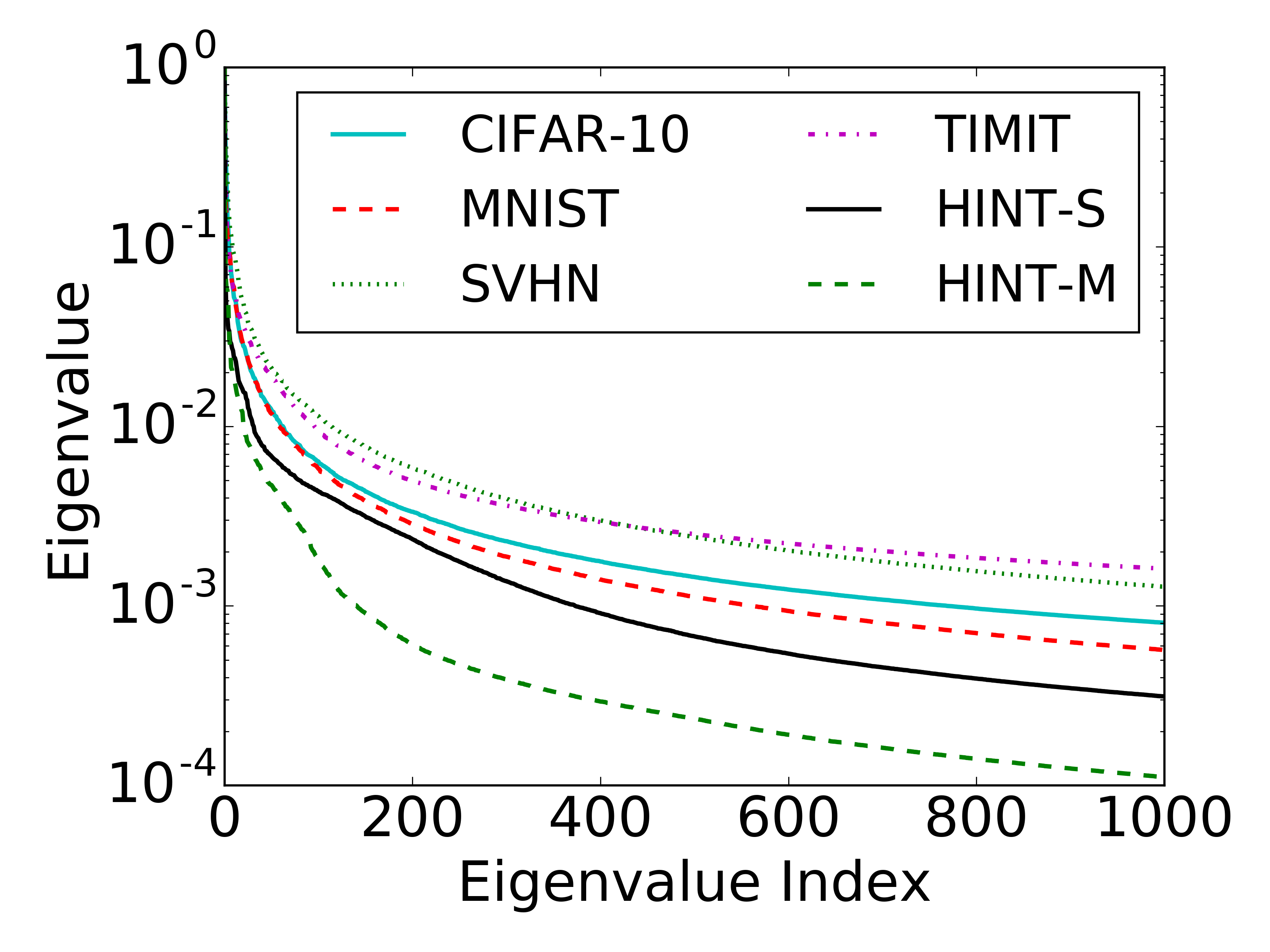
(a) Different datasets, subsample size $N=2\cdot 10^{4}$

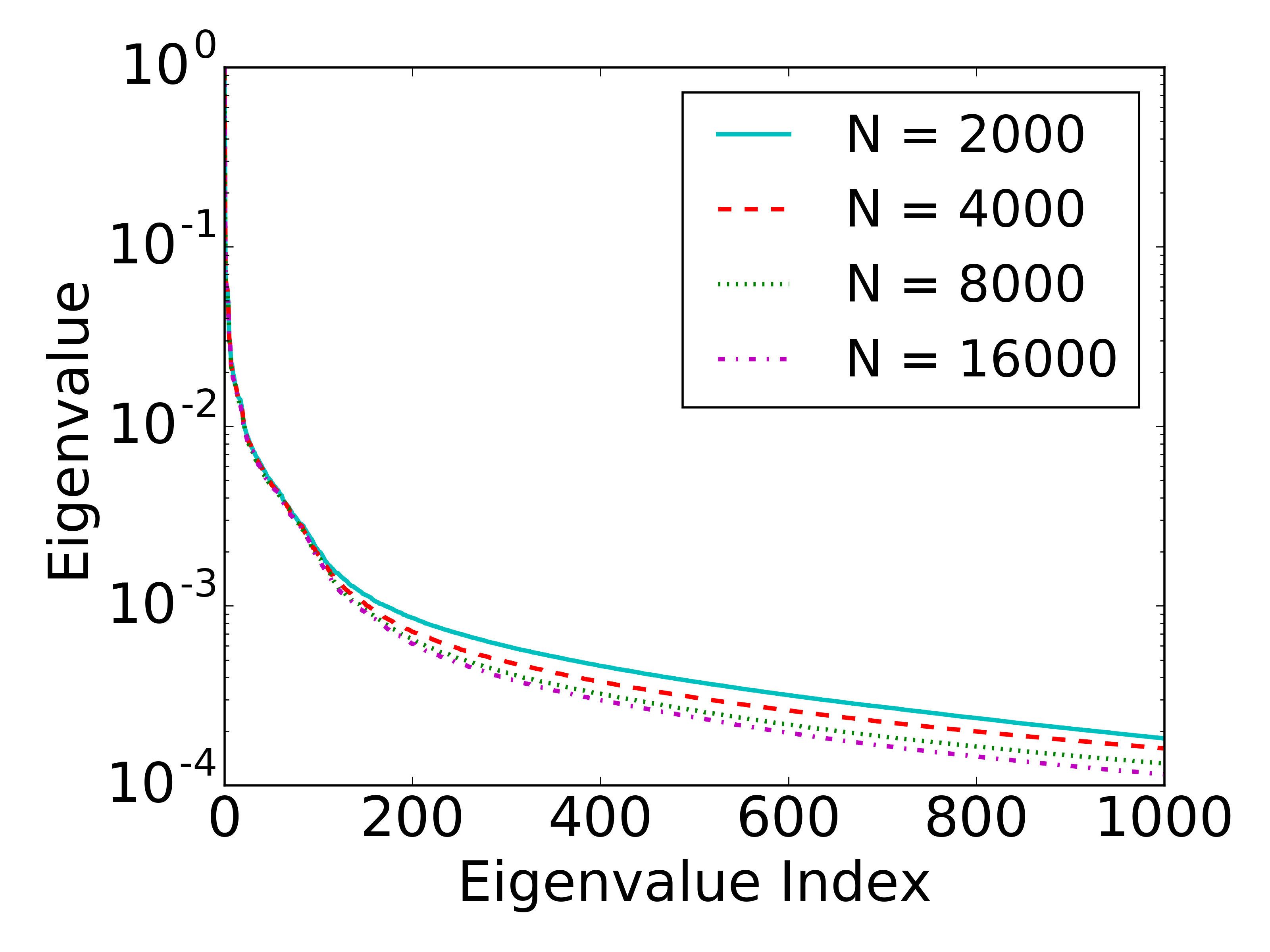
(b) Same data set, subsets of different sizes ($N$)

Figure 3: Eigenspectrum of the kernel matrices

Appendix G Eigenvalues of (Gaussian) kernel matrices

Eigenvalue ratio of kernel matrices

Ratio	CIFAR	MNIST	SVHN	TIMIT	HINT-S
$\lambda_{1}/\lambda_{41}$	68	69	39	45	128
$\lambda_{1}/\lambda_{81}$	128	135	72	84	200
$\lambda_{1}/\lambda_{161}$	245	280	138	166	338
$\lambda_{1}/\lambda_{321}$	464	567	270	290	800

For each dataset, the eigenspectrum of the corresponding kernel matrix directly determines the impact of EigenPro on convergence. Figure 3(a) shows the normalized eigenspectra ($\lambda_{i}/\lambda_{1}$) of these kernel matrices. We see that the spectrum of each dataset drops sharply for the $200$ eigenvalues, making EigenPro highly effective. Table above lists the eigenvalue ratios corresponding to different $k$. For example, with $k=160$, EigenPro for RF can in theory increase the step accelerate training by a factor of $338$ for training on HINT-S. Actual acceleration is not as large but still significant. Note that given small subsample size we expect that lower eigenvalues are probably not reflective of the full large kernel matrix. Still, even lower eigenvalues match closely when computed from subsamples of different size (Figure 3(b)).

Appendix H Kernel bandwidth selection

Here we investigate the impact of kernel bandwidth selection over convergence and performance. Table 8 compares Pegasos and EigenPro iteration using Gaussian kernel with three different bandwidths $\sigma^{2}$. When $\sigma^{2}=25$, EigenPro reaches best error rate 1.20% on testing data after 20 epochs training. Using a smaller bandwidth $\sigma^{2}=5$, EigenPro reaches its optimal in only 5 epochs. But its error rate 1.83% is significantly worse than that of $\sigma^{2}=25$. In sum, using smaller kernel bandwidth leads to slower eigenvalue decay, which in turn improves convergence of gradient-based methods. While selecting bandwidth for faster convergence does not guarantee better generalization performance (as shown in Table 8).

Table 8: Impact of kernel bandwidth on classification error and L2 loss (MNIST)

$\sigma^{2}$ $N_{Epoch}$ EigenPro Pegasos c-error L2 loss c-error L2 loss train test train test train test train test 50 1 1.58% 2.39% 3.4e-2 4.0e-2 7.29% 6.86% 9.0e-2 8.8e-2 5 0.41% 1.66% 1.7e-2 2.9e-2 3.96% 4.17% 5.7e-2 5.7e-2 10 0.15% 1.48% 1.1e-2 2.6e-2 2.92% 3.36% 4.7e-2 4.9e-2 20 0.06% 1.41% 6.6e-3 2.4e-2 2.12% 2.66% 3.8e-2 4.2e-2 40 0.01% 1.25% 3.3e-3 2.4e-2 1.45% 2.18% 3.0e-2 3.6e-2 25 1 0.92% 2.03% 2.4e-2 3.2e-2 5.12% 5.21% 6.9e-2 6.8e-2 5 0.10% 1.44% 8.6e-3 2.4e-2 2.36% 2.84% 4.0e-2 4.3e-2 10 0.01% 1.23% 4.3e-3 2.2e-2 1.58% 2.32% 3.1e-2 3.6e-2 20 0.0% 1.20% 1.8e-3 2.1e-2 0.90% 1.93% 2.3e-2 3.1e-2 40 0.0% 1.20% 6.1e-4 2.1e-2 0.39% 1.65% 1.6e-2 2.7e-2 5 1 0.01% 1.85% 2.0e-1 6.9e-2 0.37% 3.42% 1.2e-1 1.9e-1 5 0.01% 1.83% 5.9e-2 9.3e-2 0.0% 2.31% 1.0e-2 1.1e-1 10 0.0% 2.31% 1.3e-2 1.1e-1 0.0% 2.10% 1.1e-3 1.0e-1 20 0.0% 2.11% 6.0e-4 1.0e-1 0.0% 2.06% 1.0e-4 1.0e-1 40 0.0% 2.09% 0 1.0e-1 0.0% 2.07% 0 1.0e-1

References

- [ABH16] N. Agarwal, B. Bullins, and E. Hazan. Second order stochastic optimization in linear time. arXiv preprint arXiv:1602.03943, 2016.
- [ACW16] H. Avron, K. Clarkson, and D. Woodruff. Faster kernel ridge regression using sketching and preconditioning. arXiv preprint arXiv:1611.03220, 2016.
- [Aro50] N. Aronszajn. Theory of reproducing kernels. Transactions of the American mathematical society, 68(3):337–404, 1950.
- [B+05] M. L. Braun et al. Spectral properties of the kernel matrix and their relation to kernel methods in machine learning. PhD thesis, University of Bonn, 2005.
- [B+15] S. Bubeck et al. Convex optimization: Algorithms and complexity. Foundations and Trends in Machine Learning, 8(3-4):231–357, 2015.
- [BBG09] A. Bordes, L. Bottou, and P. Gallinari. SGD-QN: Careful quasi-newton stochastic gradient descent. JMLR, 10:1737–1754, 2009.
- [BE02] O. Bousquet and A. Elisseeff. Stability and generalization. JMLR, 2:499–526, 2002.
- [BHNS16] R. H. Byrd, S. Hansen, J. Nocedal, and Y. Singer. A stochastic quasi-newton method for large-scale optimization. SIAM Journal on Optimization, 26(2):1008–1031, 2016.
- [Bis07] C. Bishop. Pattern recognition and machine learning. Springer, New York, 2007.
- [BSW14] P. Baldi, P. Sadowski, and D. Whiteson. Searching for exotic particles in high-energy physics with deep learning. Nature communications, 5, 2014.
- [BV04] S. Boyd and L. Vandenberghe. Convex optimization. Cambridge university press, 2004.
- [CARR16] R. Camoriano, T. Angles, A. Rudi, and L. Rosasco. NYTRO: When subsampling meets early stopping. In AISTATS, pages 1403–1411, 2016.
- [CAS16] J. Chen, H. Avron, and V. Sindhwani. Hierarchically compositional kernels for scalable nonparametric learning. arXiv preprint arXiv:1608.00860, 2016.
- [CK11] C.-C. Cheng and B. Kingsbury. Arccosine kernels: Acoustic modeling with infinite neural networks. In ICASSP, pages 5200–5203. IEEE, 2011.
- [COCF16] K. Cutajar, M. Osborne, J. Cunningham, and M. Filippone. Preconditioning kernel matrices. In ICML, pages 2529–2538, 2016.
- [DHS11] J. Duchi, E. Hazan, and Y. Singer. Adaptive subgradient methods for online learning and stochastic optimization. JMLR, 12:2121–2159, 2011.
- [DJS96] J. E. Dennis Jr and R. B. Schnabel. Numerical methods for unconstrained optimization and nonlinear equations. SIAM, 1996.
- [DXH+14] B. Dai, B. Xie, N. He, Y. Liang, A. Raj, M. Balcan, and L. Song. Scalable kernel methods via doubly stochastic gradients. In NIPS, pages 3041–3049, 2014.
- [EM15] M. A. Erdogdu and A. Montanari. Convergence rates of sub-sampled newton methods. In NIPS, pages 3052–3060, 2015.
- [FM12] G. Fasshauer and M. McCourt. Stable evaluation of gaussian radial basis function interpolants. SIAM Journal on Scientific Computing, 34(2):A737–A762, 2012.
- [GLF+93] J. S. Garofolo, L. F. Lamel, W. M. Fisher, J. G. Fiscus, and D. S. Pallett. Darpa timit acoustic-phonetic continous speech corpus cd-rom. NIST speech disc, 1-1.1, 1993.
- [GOSS16] A. Gonen, F. Orabona, and S. Shalev-Shwartz. Solving ridge regression using sketched preconditioned svrg. In ICML, pages 1397–1405, 2016.
- [HAS+14] P.-S. Huang, H. Avron, T. N. Sainath, V. Sindhwani, and B. Ramabhadran. Kernel methods match deep neural networks on timit. In ICASSP, pages 205–209. IEEE, 2014.
- [HCL+08] C.-J. Hsieh, K.-W. Chang, C.-J. Lin, S. S. Keerthi, and S. Sundararajan. A dual coordinate descent method for large-scale linear svm. In ICML, pages 408–415, 2008.
- [HMT11] N. Halko, P.-G. Martinsson, and J. A. Tropp. Finding structure with randomness: Probabilistic algorithms for constructing approximate matrix decompositions. SIAM review, 53(2):217–288, 2011.
- [HYWW13] E. W. Healy, S. E. Yoho, Y. Wang, and D. Wang. An algorithm to improve speech recognition in noise for hearing-impaired listeners. The Journal of the Acoustical Society of America, 134(4):3029–3038, 2013.
- [JZ13] R. Johnson and T. Zhang. Accelerating stochastic gradient descent using predictive variance reduction. In NIPS, pages 315–323, 2013.
- [KB14] D. Kingma and J. Ba. Adam: A method for stochastic optimization. arXiv preprint arXiv:1412.6980, 2014.
- [KH09] A. Krizhevsky and G. Hinton. Learning multiple layers of features from tiny images. Master’s thesis, University of Toronto, 2009.
- [KSW04] J. Kivinen, A. J. Smola, and R. C. Williamson. Online learning with kernels. Signal Processing, IEEE Transactions on, 52(8):2165–2176, 2004.
- [Küh87] T. Kühn. Eigenvalues of integral operators with smooth positive definite kernels. Archiv der Mathematik, 49(6):525–534, 1987.
- [LBBH98] Y. LeCun, L. Bottou, Y. Bengio, and P. Haffner. Gradient-based learning applied to document recognition. In Proceedings of the IEEE, volume 86, pages 2278–2324, 1998.
- [LML+14] Z. Lu, A. May, K. Liu, A. B. Garakani, D. Guo, A. Bellet, L. Fan, M. Collins, B. Kingsbury, M. Picheny, and F. Sha. How to scale up kernel methods to be as good as deep neural nets. arXiv preprint arXiv:1411.4000, 2014.
- [LN89] D. C. Liu and J. Nocedal. On the limited memory bfgs method for large scale optimization. Mathematical programming, 45(1-3):503–528, 1989.
- [LSS13] Q. Le, T. Sarlós, and A. Smola. Fastfood-approximating kernel expansions in loglinear time. In ICML, 2013.
- [MDFFF16] S.-M. Moosavi-Dezfooli, A. Fawzi, O. Fawzi, and P. Frossard. Universal adversarial perturbations. arXiv preprint arXiv:1610.08401, 2016.
- [MGL+17] A. May, A. B. Garakani, Z. Lu, D. Guo, K. Liu, A. Bellet, L. Fan, M. Collins, D. Hsu, B. Kingsbury, et al. Kernel approximation methods for speech recognition. arXiv preprint arXiv:1701.03577, 2017.
- [Min17] S. Minsker. On some extensions of bernstein’s inequality for self-adjoint operators. Statistics & Probability Letters, 2017.
- [MNJ16] P. Moritz, R. Nishihara, and M. Jordan. A linearly-convergent stochastic l-bfgs algorithm. In AISTATS, pages 249–258, 2016.
- [Mur98] N. Murata. A statistical study of on-line learning. Online Learning and Neural Networks. Cambridge University Press, Cambridge, UK, pages 63–92, 1998.
- [NWC+11] Y. Netzer, T. Wang, A. Coates, A. Bissacco, B. Wu, and A. Ng. Reading digits in natural images with unsupervised feature learning. In NIPS workshop, volume 2011, page 4, 2011.
- [PGB+11] D. Povey, A. Ghoshal, G. Boulianne, L. Burget, O. Glembek, N. Goel, M. Hannemann, P. Motlicek, Y. Qian, P. Schwarz, et al. The kaldi speech recognition toolkit. In ASRU, 2011.
- [QB16] Q. Que and M. Belkin. Back to the future: Radial basis function networks revisited. In AISTATS, pages 1375–1383, 2016.
- [RBV10] L. Rosasco, M. Belkin, and E. D. Vito. On learning with integral operators. JMLR, 11(Feb):905–934, 2010.
- [Ric11] L. F. Richardson. The approximate arithmetical solution by finite differences of physical problems involving differential equations, with an application to the stresses in a masonry dam. Philosophical Transactions of the Royal Society of London. Series A, 210:307–357, 1911.
- [Ros97] S. Rosenberg. The Laplacian on a Riemannian manifold: an introduction to analysis on manifolds. Cambridge University Press, 1997.
- [RR07] A. Rahimi and B. Recht. Random features for large-scale kernel machines. In NIPS, pages 1177–1184, 2007.
- [RSB12] N. L. Roux, M. Schmidt, and F. R. Bach. A stochastic gradient method with an exponential convergence _rate for finite training sets. In NIPS, pages 2663–2671, 2012.
- [RWY14] G. Raskutti, M. Wainwright, and B. Yu. Early stopping and non-parametric regression: an optimal data-dependent stopping rule. JMLR, 15(1):335–366, 2014.
- [SC08] I. Steinwart and A. Christmann. Support vector machines. Springer Science & Business Media, 2008.
- [She94] J. R. Shewchuk. An introduction to the conjugate gradient method without the agonizing pain. Technical report, Pittsburgh, PA, USA, 1994.
- [SNB05] V. Sindhwani, P. Niyogi, and M. Belkin. Beyond the point cloud: from transductive to semi-supervised learning. In ICML, pages 824–831, 2005.
- [SS16] G. Santin and R. Schaback. Approximation of eigenfunctions in kernel-based spaces. Advances in Computational Mathematics, 42(4):973–993, 2016.
- [SSSSC11] S. Shalev-Shwartz, Y. Singer, N. Srebro, and A. Cotter. Pegasos: Primal estimated sub-gradient solver for SVM. Mathematical programming, 127(1):3–30, 2011.
- [STC04] J. Shawe-Taylor and N. Cristianini. Kernel methods for pattern analysis. Cambridge university press, 2004.
- [SYG07] N. N. Schraudolph, J. Yu, and S. Günter. A stochastic quasi-newton method for online convex optimization. In AISTATS, pages 436–443, 2007.
- [SZS+13] C. Szegedy, W. Zaremba, I. Sutskever, J. Bruna, D. Erhan, I. Goodfellow, and R. Fergus. Intriguing properties of neural networks. arXiv preprint arXiv:1312.6199, 2013.
- [TBRS13] M. Takác, A. S. Bijral, P. Richtárik, and N. Srebro. Mini-batch primal and dual methods for SVMs. In ICML (3), pages 1022–1030, 2013.
- [TH12] T. Tieleman and G. Hinton. Lecture 6.5-rmsprop: Divide the gradient by a running average of its recent magnitude. COURSERA: Neural Networks for Machine Learning, 4:2, 2012.
- [Tro15] J. A. Tropp. An introduction to matrix concentration inequalities. arXiv preprint arXiv:1501.01571, 2015.
- [TRVR16] S. Tu, R. Roelofs, S. Venkataraman, and B. Recht. Large scale kernel learning using block coordinate descent. arXiv preprint arXiv:1602.05310, 2016.
- [Tsy04] A. B. Tsybakov. Optimal aggregation of classifiers in statistical learning. Annals of Statistics, pages 135–166, 2004.
- [WS01] C. Williams and M. Seeger. Using the Nyström method to speed up kernel machines. In NIPS, pages 682–688, 2001.
- [YRC07] Y. Yao, L. Rosasco, and A. Caponnetto. On early stopping in gradient descent learning. Constructive Approximation, 26(2):289–315, 2007.
- [ZBH+16] C. Zhang, S. Bengio, M. Hardt, B. Recht, and O. Vinyals. Understanding deep learning requires rethinking generalization. arXiv preprint arXiv:1611.03530, 2016.