A moving control volume approach to computing hydrodynamic forces and torques on immersed bodies

Abstract

We present a moving control volume (CV) approach to computing hydrodynamic forces and torques on complex geometries. The method requires surface and volumetric integrals over a simple and regular Cartesian box that moves with an arbitrary velocity to enclose the body at all times. The moving box is aligned with Cartesian grid faces, which makes the integral evaluation straightforward in an immersed boundary (IB) framework. Discontinuous and noisy derivatives of velocity and pressure at the fluid-structure interface are avoided and far-field (smooth) velocity and pressure information is used. We re-visit the approach to compute hydrodynamic forces and torques through force/torque balance equation in a Lagrangian frame that some of us took in a prior work (Bhalla et al., J Comp Phys, 2013). We prove the equivalence of the two approaches for IB methods, thanks to the use of Peskin’s delta functions. Both approaches are able to suppress spurious force oscillations and are in excellent agreement, as expected theoretically. Test cases ranging from Stokes to high Reynolds number regimes are considered. We discuss regridding issues for the moving CV method in an adaptive mesh refinement (AMR) context. The proposed moving CV method is not limited to a specific IB method and can also be used, for example, with embedded boundary methods.

1 Introduction

Fluid-structure interaction (FSI) problems involving moving bodies is a challenging area in the computational fluid dynamics field that has vested the interest of researchers for several decades. FSI modeling has traditionally been carried out in two ways: the body-fitted mesh approach using unstructured grids [1, 2] and the Cartesian grid approach based on the fictitious domain method [3, 4]. Although the body-fitted mesh approach to FSI resolves the fluid-structure interface sharply, it requires complex mesh management infrastructure along with high computational costs for solving linear equations. The fictitious domain method on the other hand extends the fluid equations inside the structure along with some additional non-zero body forcing term. As a result, regular Cartesian grids and fast linear solvers such as fast Fourier transform can be used to solve the common momentum equation of the continua. However, fictitious domain methods tend to smear the fluid-structure interface and hence reduce the solution accuracy near the interface.

One widely used fictitious domain approach to FSI is the immersed boundary (IB) method [5] which was originally proposed by Peskin in the context of cardiac flows [6]. The main advantage to IB methods is that they do not require a body-fitted mesh to model the structure. The immersed body is allowed to freely cut the background Cartesian mesh, making the IB method easy to implement within an existing incompressible flow solver. A Lagrangian force density is computed on structure nodes, which is then transferred to the background grid via regularized delta functions. The use of regularized delta functions diffuses the interface and smears it over a number of grid cells proportional to the width of the delta function. This often leads to discontinuous or noisy derivatives of the velocity and pressure field required to compute surface traction.

The original IB method uses an explicit time stepping scheme and fiber elasticity to compute the additional body forcing inside the region occupied by the structure. The method works fairly well for soft elastic structures, but incurs severe time step restrictions if the stiffness of the material is substantially increased to model rigid bodies. Specialized versions of the original IB method have been developed to model rigid and stiff bodies in an efficient manner like the implicit IB method [7, 8, 9, 10, 11], the direct forcing method [12, 13, 14], and the fully constrained IB method [15, 16, 17]. The implicit IB method requires special solvers like algebraic [18] and geometric multigrid [7, 10] to treat the stiff elastic forces implicitly. The direct forcing and fully constrained IB methods that are primarily used for modeling rigid bodies impose rigidity constraint through Lagrange multipliers. The direct forcing method approximates the Lagrange multiplier with suitable penalty term and solves the fluid-structure equations in a fractional time stepping scheme. This is in contrast to fully constrained IB method where the fluid velocity, pressure, and Lagrange multipliers are solved together. Apart from the obvious advantage of imposing the rigidity constraint exactly rather approximately, the fully constrained IB method can be used for Stokes flow where fractional time stepping schemes do not work. However, special preconditioners are required to solve for the Lagrange multipliers exactly [16, 17], which makes solving the system costly for big three dimensional volumetric bodies.

A common feature of IB methods that are based on Peskin’s IB approach [5] is that they do not require rich geometric information like surface elements and normals to compute the Lagrangian force density. Structure node position (and possibly the node connectivity) information suffices to compute Lagrangian forces. However, there are many other versions of the IB method and Cartesian grid based methods that require additional geometric information to sharply resolve the fluid-structure interface. Examples include the immersed finite element method [19, 20, 21, 22], the immersed interface method [23, 24], the ghost-fluid method [25], and the cut-cell embedded boundary method [26, 27, 28]. For such approaches, the availability of surface elements and normals along with sharp interface resolution makes the surface traction computation easier and smooth (for at least smooth problems).

Often times, the net hydrodynamic forces and torques on immersed bodies are desired rather than point-wise traction values. Force/torque balance equations can be used to compute the hydrodynamic force/torque contribution instead of directly integrating surface traction. In the context of “Peskin-like” IB methods, this implies that one can essentially eliminate surface mesh generation as a post-processing step if only net hydrodynamic forces and torques are desired. This has another added advantage of not using noisy derivatives of velocity and pressure at the interface for evaluating hydrodynamic forces and torques.

In this work we analyze and compare two approaches to computing net hydrodynamic forces and torques on an immersed body. In the first approach we use the Reynolds transport theorem (RTT) to convert the traction integral over an irregular body surface to a traction integral over a regular and simple Cartesian box (that is aligned with grid faces). The RTT is proposed for a moving control volume that translates with an arbitrary velocity to enclose the immersed body at all times. We refer to this approach as the moving CV approach. In the context of locally refined grids, the moving control volume can span a hierarchy of grid levels. In the second approach, hydrodynamic forces and torques are computed using inertia and Lagrange multipliers (approximate or exact) defined in the body region. We refer to this approach as the LM approach and has been used before in [13]. For IB methods, we show that both approaches are equivalent. This is due to a special property of Peskin’s delta functions that makes Lagrangian and Eulerian force density equivalent [5]. We show that both these approaches give smooth forces and suppress spurious oscillations that arise by directly integrating spatial pressure and velocity gradients over the immersed body as reported in the literature [29].

Although application of the RTT on a stationary control volume to evaluate hydrodynamic force is a well known result [30, 31]; its extension to moving control volumes was first proposed by Flavio Noca in 1997 [32]. They were motivated by the task of evaluating net hydrodynamic force on a moving bluff body using DPIV data from experiments. Flavio has also proposed force expressions that eliminate the pressure variable; a quantity not available in DPIV experiments [32, 33]. We do not analyze such expressions in this work, however. In the context of IB method, Bergmann and co-workers [34, 35] have used Flavio’s moving control volume force expressions (involving both velocity and pressure) to compute hydrodynamic forces. They observed spurious force oscillations with a moving control volume approach [34]. We show that by manipulating time derivatives in the original expressions, one can eliminate such spurious oscillations. We also present strategies to mitigate jumps in velocity derivatives in an AMR framework. Such jumps arise when the Cartesian grid hierarchy is regridded and velocity in the new grid hierarchy is reconstructed from the old hierarchy [36]. Lai and Peskin [37] used stationary control volume analysis on a uniform grid to compute steady state hydrodynamic forces on a stationary cylinder for Reynolds numbers between $100-200$ using the IB method. They did not consider time derivative terms in their analysis and temporal hydrodynamic force profiles were reported at steady state. In this work we include time derivative terms for finite Reynolds number flows (but not for steady Stokes flow) in our (moving) control volume analysis.

If point-wise traction values are desired for IB-like methods, there are several recommendations proposed in the literature for smoothing them. Here we list a few of them. Verma et al. [38] have recommended using a “lifted” surface: a surface two grid cell distance away from the actual interface to avoid choppy velocity gradients. This recommendation, based upon their empirical tests using a Brinkman penalization method, can change depending on the smoothness of the problem and the discrete delta function used in IB methods. Goza et al. [39] obtain smooth point-wise force measurements by using a force filtering post-processing step that penalizes inaccurate high frequency stress components. Martins et al. [40] enforce a continuity constraint in the velocity interpolation stencil to reconstruct a second-order velocity field at IB surface points that is discretely divergence-free. They also impose a normal gradient constraint in the pressure interpolation stencil to reconstruct a second-order accurate pressure field at IB points. They have successfully eliminated spurious force oscillations using constrained least-squares stencils. The idea of unconstrained moving least-squares velocity interpolation and force spreading in the context of direct forcing IB method was first proposed by Vanella and Balaras [41]. Lee et al. [29] attribute sources of spurious force oscillations to spatial pressure discontinuities across the fluid-solid interface and temporal velocity discontinuities for moving bodies. They recommend using fine grid resolutions to alleviate spurious oscillations. Their analyses and tests [29] show that grid spacing has a more pronounced effect on spurious force oscillations than computational time step size.

For a range of test cases varying from free-swimming at high Reynolds number to steady Stokes flow, we show that both LM and moving CV methods are in excellent agreement and are able to suppress spurious force oscillations. They do not require any additional treatment such as least-squares stencil (velocity and pressure) interpolation or force filtering beyond simple integration of force balance laws. For moderate to high Reynolds number test cases, we use a direct forcing IB method to estimate Lagrange multipliers, and for Stokes flow we use a fully constrained IB method to compute Lagrange multipliers exactly.

2 Equations of motion

2.1 Immersed boundary method

The immersed boundary (IB) formulation uses an Eulerian description for the momentum equation and divergence-free condition for both the fluid and the structure. A Lagrangian description is employed for the structural position and forces. Let $\bm{\mathrm{x}}=(x_{1},\ldots,x_{d})\in\Omega$ denote fixed Cartesian coordinates, in which $\Omega\subset\mathbb{R}^{d}$ is the fixed domain occupied by the entire fluid-structure system in $d$ spatial dimensions. Let $\bm{\mathrm{s}}=(s_{1},\ldots s_{d})\in U$ denote the fixed material coordinate system attached to the structure, in which $U\subset\mathbb{R}^{d}$ is the Lagrangian curvilinear coordinate domain. The position of the immersed structure occupying a volumetric region $V_{b}(t)\subset\Omega$ at time $t$ is denoted by $\bm{\mathrm{X}}(\bm{\mathrm{s}},t)$. We consider only neutrally buoyant bodies to simplify the implementation; this assumption implies that the fluid and structure share the same uniform mass density $\rho$. The deviatoric stress tensor of fluid, characterized by dynamic viscosity $\mu$, is extended inside the structure to make the momentum equation of both media appear similar. The combined equations of motion for fluid-structure system are [5]

$$\rho\left(\frac{\partial\bm{\mathrm{u}}}{\partial t}(\bm{\mathrm{x}},t)+\bm{\mathrm{u}}(\bm{\mathrm{x}},t)\cdot\nabla\bm{\mathrm{u}}(\bm{\mathrm{x}},t)\right) =-\nabla p(\bm{\mathrm{x}},t)+\mu\nabla^{2}\bm{\mathrm{u}}(\bm{\mathrm{x}},t)+\bm{\mathrm{f}}(\bm{\mathrm{x}},t),$$ (1)

$$\nabla\cdot\mbox{}\bm{\mathrm{u}}(\bm{\mathrm{x}},t) =0,$$ (2)

$$\bm{\mathrm{f}}(\bm{\mathrm{x}},t) =\int_{U}\bm{\mathrm{F}}(\bm{\mathrm{s}},t)\,\delta(\bm{\mathrm{x}}-\bm{\mathrm{X}}(\bm{\mathrm{s}},t))\,{\mathrm{d}}\bm{\mathrm{s}},$$ (3)

$$\bm{\mathrm{U}}(\bm{\mathrm{s}},t) =\int_{\Omega}\bm{\mathrm{u}}(\bm{\mathrm{x}},t)\,\delta(\bm{\mathrm{x}}-\bm{\mathrm{X}}(\bm{\mathrm{s}},t))\,{\mathrm{d}}\bm{\mathrm{x}},$$ (4)

$$\frac{\partial\bm{\mathrm{X}}}{\partial t}(\bm{\mathrm{s}},t) =\bm{\mathrm{U}}(\bm{\mathrm{s}},t).$$ (5)

Eqs. (1) and (2) are the incompressible Navier-Stokes equations written in Eulerian form, in which $\bm{\mathrm{u}}(\bm{\mathrm{x}},t)$ is the velocity, $p(\bm{\mathrm{x}},t)$ is the pressure, and $\bm{\mathrm{f}}(\bm{\mathrm{x}},t)$ is the Eulerian force density, which is non-zero only in the structure region. Interactions between Lagrangian and Eulerian quantities in Eqs. (3) and (4) are mediated by integral equations with Dirac delta function kernels, in which the $d$-dimensional delta function is $\delta(\bm{\mathrm{x}})=\Pi_{i=1}^{d}\delta(x_{i})$. Eq. (3) converts the Lagrangian force density $\bm{\mathrm{F}}(\bm{\mathrm{s}},t)$ into an equivalent Eulerian density $\bm{\mathrm{f}}(\bm{\mathrm{x}},t)$. In the IB literature, the discretized version of this operation is called force spreading. Using short-hand notation, we denote force spreading operation by $\bm{\mathrm{f}}=\bm{\mathrm{\mathcal{S}}}[\bm{\mathrm{X}}]\,\bm{\mathrm{F}}$, in which $\bm{\mathrm{\mathcal{S}}}[\bm{\mathrm{X}}]$ is the force-spreading operator. Eq. (4) determines the physical velocity of each Lagrangian material point from the Eulerian velocity field, so that the immersed structure moves according to the local value of the velocity field $\bm{\mathrm{u}}(\bm{\mathrm{x}},t)$ (Eq. (5)). This velocity interpolation operation is expressed as $\frac{\partial\bm{\mathrm{X}}}{\partial t}=\bm{\mathrm{U}}=\bm{\mathrm{\mathcal{J}}}[\bm{\mathrm{X}}]\,\bm{\mathrm{u}}$, in which $\bm{\mathrm{\mathcal{J}}}[\bm{\mathrm{X}}]$ is the velocity-interpolation operator. It can be shown that if $\bm{\mathrm{\mathcal{S}}}$ and $\bm{\mathrm{\mathcal{J}}}$ are taken to be adjoint operators, i.e. $\bm{\mathrm{\mathcal{S}}}=\bm{\mathrm{\mathcal{J}}}^{*}$, then Lagrangian-Eulerian coupling conserves energy [5].

2.2 Discrete equations of motion

We employ a staggered grid discretization for the momentum and continuity equations (see Fig. 2). More specifically, Eulerian velocity and force variables are defined at face centers while the pressure variable is defined at cell centers. Second-order finite difference stencils are used to spatially discretize the Eulerian equations on locally refined grids [13, 36]. The spatial discretization of various operators are denoted with $h$ subscripts. To discretize equations in time, we take $\Delta t$ as the time step size, and $n$ as the time step number. We use the direct forcing method of Bhalla et al. [13] for moderate to high Reynolds number cases and the fully constrained IB method of Kallemov et al. [16] for Stokes flow cases. The two methods differ in how the Lagrangian force density or Lagrange multipliers are computed. The time integrators are also different for the two methods. Here we briefly describe the discretized equations for both methods. We refer readers to [13, 16, 17] for more details.

For the direct forcing method, the time stepping scheme reads as [13]

$$\rho\left(\frac{\tilde{\bm{\mathrm{u}}}^{n+1}-\bm{\mathrm{u}}^{n}}{\Delta t}+[\bm{\mathrm{u}}\cdot\nabla_{h}\bm{\mathrm{u}}]^{(n+\frac{1}{2})}\right) =-\nabla_{h}p^{n+\frac{1}{2}}+\frac{\mu}{2}\bm{\mathrm{\nabla}}^{2}_{h}\left(\tilde{\bm{\mathrm{u}}}^{n+1}+\bm{\mathrm{u}}^{n}\right),$$ (6)

$$\nabla_{h}\cdot\tilde{\bm{\mathrm{u}}}^{n+1} =\bm{\mathrm{0}},$$ (7)

$$\bm{\mathrm{F}}^{n+\frac{1}{2}} =\frac{\rho}{\Delta t}\left(\bm{\mathrm{U}}_{b}^{n+1}-\bm{\mathrm{\mathcal{J}}}_{h}[\bm{\mathrm{X}}^{n+\frac{1}{2}}]\tilde{\bm{\mathrm{u}}}^{n+1}\right),$$ (8)

$$\rho\left(\frac{\bm{\mathrm{u}}^{n+1}-\tilde{\bm{\mathrm{u}}}^{n+1}}{\Delta t}\right) =\bm{\mathrm{\mathcal{S}}}_{h}[\bm{\mathrm{X}}^{n+\frac{1}{2}}]\bm{\mathrm{F}}^{n+\frac{1}{2}}.$$ (9)

Succinctly, we first solve for a velocity field $\tilde{\bm{\mathrm{u}}}^{n+1}$ and a pressure field $p^{n+\frac{1}{2}}$ as a coupled system by solving Eqs. (6) and (7) simultaneously. The velocity $\tilde{\bm{\mathrm{u}}}^{n+1}$, which is correct in the fluid region but not in the structure region $V_{b}(t)$, is then corrected by estimating the Lagrange multiplier $\bm{\mathrm{F}}^{n+\frac{1}{2}}$ via Eq. (8). Here $\bm{\mathrm{U}}_{b}^{n+1}$ is the desired rigid body velocity of the Lagrangian nodes, and $\bm{\mathrm{X}}^{n+\frac{1}{2}}$ is the midstep estimate of Lagrangian node position. Finally, the Lagrange multiplier $\bm{\mathrm{F}}^{n+\frac{1}{2}}$ is spread on the background grid to correct the momentum in the structure region to $\bm{\mathrm{u}}^{n+1}$. We use Adams-Bashforth to approximate the midstep value of nonlinear convection term $\bm{\mathrm{u}}\cdot\nabla\bm{\mathrm{u}}$ via

$$[\bm{\mathrm{u}}\cdot\nabla_{h}\bm{\mathrm{u}}]^{(n+\frac{1}{2})}=\frac{3}{2}\bm{\mathrm{u}}^{n}\cdot\nabla_{h}\bm{\mathrm{u}}^{n}-\frac{1}{2}\bm{\mathrm{u}}^{n-1}\cdot\nabla_{h}\bm{\mathrm{u}}^{n-1}.$$ (10)

For the fully constrained method, we simultaneously solve for the updated Eulerian velocity $\bm{\mathrm{u}}^{n+1}$ and pressure $p^{n+1}$ at time $t^{n+1}$ along with the Lagrange multiplier $\bm{\mathrm{F}}^{n+1}$. The time stepping scheme reads as [16, 17]

$$-\nabla_{h}p^{n+1}+\mu\bm{\mathrm{\nabla}}^{2}_{h}\bm{\mathrm{u}}^{n+1}+\bm{\mathrm{\mathcal{S}}}_{h}[\bm{\mathrm{X}}^{n}]\bm{\mathrm{F}}^{n+1} =\bm{\mathrm{0}},$$ (11)

$$\nabla_{h}\cdot\bm{\mathrm{u}}^{n+1} =\bm{\mathrm{0}},$$ (12)

$$\bm{\mathrm{\mathcal{J}}}_{h}[\bm{\mathrm{X}}^{n}]\bm{\mathrm{u}}^{n+1} =\bm{\mathrm{U}}_{b}^{n+1}.$$ (13)

The coupled system of Eqs. (11)-(13) is solved simultaneously using a preconditioned FGMRES [42] solver. For both methods, we update the Lagrangian node positions $\bm{\mathrm{X}}^{n+1}$ using rigid body translation and rotation. We use Peskin’s 4-point regularized delta functions for the $\bm{\mathrm{\mathcal{S}}}$ and $\bm{\mathrm{\mathcal{J}}}$ operators in all our numerical experiments, unless stated otherwise.

Our finite Reynolds number fluid solver has support for adaptive mesh refinement, and some cases presented in Sec. 5 make use of multiple grid levels (also known as a grid hierarchy). A grid with $\ell$ refinement levels with grid spacing $\Delta x_{0}$, $\Delta y_{0}$, and $\Delta z_{0}$ on the coarsest grid level has minimum grid spacing $\Delta x_{\textrm{min}}=\Delta x_{0}/n_{\text{ref}}^{\ell-1}$, $\Delta y_{\textrm{min}}=\Delta y_{0}/n_{\text{ref}}^{\ell-1}$, and $\Delta z_{\textrm{min}}=\Delta z_{0}/n_{\text{ref}}^{\ell-1}$ on the finest grid level. Here, $n_{\text{ref}}\in\mathbb{N}$ is the refinement ratio. In the present work, the refinement ratio in taken to be the same in each direction, although this is not a limitation of the numerical method. The immersed structure is always placed on the finest grid level. For all of the cases considered in this work a constant time step size $\Delta t=\min(\Delta t^{\ell})$ is chosen, in which the time step size $\Delta t^{\ell}$ on grid level $\ell$ satisfies the convective CFL condition $\Delta t^{\ell}\leq C\min\left(\frac{\Delta x}{\|u_{x}\|_{\infty}},\frac{\Delta y}{\|u_{y}\|_{\infty}},\frac{\Delta z}{\|u_{z}\|_{\infty}}\right)^{\ell}$. In this work, the convective CFL number is set to $C=0.3$ unless otherwise stated.

3 Hydrodynamic force and torque

3.1 Moving control volume method

3.1.1 Hydrodynamic force

Letting $\bm{\mathrm{T}}=\mu\left(\nabla\bm{\mathrm{u}}+\nabla\bm{\mathrm{u}}^{T}\right)$ denote the viscous stress tensor, the net hydrodynamic force is defined to be the force of the fluid on the body:

$$\bm{\mathrm{\mathcal{F}}}(t)=-\oint_{S_{b}(t)}\bm{\mathrm{n}}\cdot\left[-p\bm{\mathrm{I}}+\bm{\mathrm{T}}\right]\,\mathrm{dS},$$ (14)

in which the integral is taken over the surface of the body $S_{b}(t)=\partial V_{b}(t)$, and $\bm{\mathrm{n}}$ is the unit outward normal to the surface. In practice, evaluating Eq. (14) is inconvenient in numerical experiments because it is often difficult to obtain accurate surface velocity gradients and pressure values. Moreover, evaluating Eq. (14) also requires computational geometry to obtain surface normals and area. Instead we use a control volume approach to compute $\bm{\mathrm{\mathcal{F}}}(t)$ which avoids these requirements.

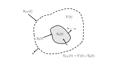
Figure 1: Sketch of the immersed structure (solid line) surrounded by an arbitrary control volume (dashed line)

.

Let an arbitrary (possibly time dependent) domain $V_{\text{CV}}(t)$ completely surround $V_{b}(t)$, i.e. $V_{b}(t)\subset V_{\text{CV}}(t)$, as shown in Fig. 1. By considering the change in momentum within the control volume $V_{\text{CV}}(t)$ and the net momentum flux at its surface $S_{\text{CV}}(t)=\partial V_{\text{CV}}(t)$, a general expression for the hydrodynamic force on the body can be obtained

$$\bm{\mathrm{\mathcal{F}}}(t)=-\frac{{\rm d}}{{\rm d}t}\int_{V(t)}\rho\bm{\mathrm{u}}\,\mathrm{dV}+\oint_{S_{\text{CV}}(t)}\bm{\mathrm{n}}\cdot\left[-p\bm{\mathrm{I}}-(\bm{\mathrm{u}}-\bm{\mathrm{u}}_{S})\rho\bm{\mathrm{u}}+\bm{\mathrm{T}}\right]\,\mathrm{dS}-\oint_{S_{b}(t)}\bm{\mathrm{n}}\cdot(\bm{\mathrm{u}}-\bm{\mathrm{u}}_{S})\rho\bm{\mathrm{u}}\,\mathrm{dS},$$ (15)

in which $V(t)=V_{\text{CV}}(t)\setminus V_{b}(t)$ is the volume outside the immersed body but inside the CV, and $\bm{\mathrm{u}}_{S}$ is the velocity of the surface over which the (surface) integral is evaluated. In general $\bm{\mathrm{u}}_{S}\neq\bm{\mathrm{u}}$, and $\bm{\mathrm{u}}_{S}$ can be arbitrarily chosen so that the moving CV always encloses the immersed body. The unit normal $\bm{\mathrm{n}}$ in Eq. (15) points outward on $S_{\text{CV}}(t)$, and into $S_{b}(t)$. The above force equation was first derived by Noca [32] and has been used in various experimental [33, 43, 44, 45] and numerical [34, 35, 46, 47] studies. For Cartesian grid based methods, the CV can be chosen as a simple rectangular domain, for which the unit normals on $S_{\text{CV}}(t)$ are aligned with the Cartesian axes. Finally, the integral over $S_{b}(t)$ vanishes for many applications where no-slip ($\bm{\mathrm{u}}_{S}=\bm{\mathrm{u}}$) boundary condition can be chosen for $\bm{\mathrm{u}}_{S}$. Henceforth, we will analyze cases for no-slip boundary conditions.

When Eq. (15) is discretized, the first term requires a discrete approximation of the integral at two separate time instances or at two different locations of the moving control volume. Bergmann et al.  [34] observed spurious force oscillations as a result of this time derivative term. We show that by manipulating the first term using the Reynolds transport theorem, an expression for hydrodynamic force can be obtained that does not require contributions from control volumes at two different spatial locations. The modified equation reads as

$$\bm{\mathrm{\mathcal{F}}}(t)=-\int_{V_{\text{CV}}(t)}\rho\frac{\partial\bm{\mathrm{u}}}{\partial t}\,\mathrm{dV}+\frac{{\rm d}}{{\rm d}t}\int_{V_{b}(t)}\rho\bm{\mathrm{u}}\,\mathrm{dV}+\oint_{S_{\text{CV}}(t)}\bm{\mathrm{n}}\cdot\left[-p\bm{\mathrm{I}}-\bm{\mathrm{u}}\rho\bm{\mathrm{u}}+\bm{\mathrm{T}}\right]\,\mathrm{dS}.$$ (16)

A detailed derivation of Eq. (16) is provided in A. Note that although Eqs. (15) and (16) are equivalent formulas to obtain the hydrodynamic force on an immersed body, their physical interpretations are different. In Eq. (15), the control volume is moving with some prescribed velocity, usually chosen to follow the structure to ensure it is contained within the CV at all times. Hence, one must keep track of the velocity $\bm{\mathrm{u}}_{S}$ of the control surface $S_{\text{CV}}(t)$. Moreover since the time derivative appears outside of the integral over $V(t)$, it requires a discrete approximation of momentum on two time-lagged control volumes. On the other hand in Eq. (16), all integrals over the control volume are evaluated at a single time instance and therefore a discrete evaluation on two separate CVs is never needed. Discretely, the control volume is placed at a new location at time step (${n+1}$) and no information from its previous location at time step $n$ is used. Hence, $\bm{\mathrm{u}}_{S}$ never appears in the calculation. This has the numerical benefit of suppressing force oscillations, which will be shown in Sec. 5.

3.1.2 Hydrodynamic torque

The net hydrodynamic torque on an immersed body is defined to be the net moment of hydrodynamic force exerted by fluid on the body about a given reference point:

$$\bm{\mathrm{\mathcal{M}}}(t)=-\oint_{S_{b}(t)}\bm{\mathrm{r}}\wedge\left(\bm{\mathrm{n}}\cdot\left[-p\bm{\mathrm{I}}+\bm{\mathrm{T}}\right]\right)\,\mathrm{dS},$$ (17)

in which $\bm{\mathrm{r}}=\bm{\mathrm{x}}-\bm{\mathrm{x}}_{0}$. The torque is computed with respect to some reference point $\bm{\mathrm{x}}_{0}$, which can be fixed at a location or move with time (e.g. the center of mass of a swimmer). Following Noca’s derivation for the force expression Eq. (15), one can measure the change in angular momentum within a moving control volume to obtain an expression for torque which reads as

$$\bm{\mathrm{\mathcal{M}}}(t)=-\frac{{\rm d}}{{\rm d}t}\int_{V(t)}(\bm{\mathrm{r}}\wedge\rho\bm{\mathrm{u}})\,\mathrm{dV}+\oint_{S_{\text{CV}}(t)}[\bm{\mathrm{r}}\wedge(-p\;\bm{\mathrm{n}}+\bm{\mathrm{n}}\cdot\bm{\mathrm{T}})-\bm{\mathrm{n}}\cdot(\bm{\mathrm{u}}-\bm{\mathrm{u}}_{S})(\bm{\mathrm{r}}\wedge\rho\bm{\mathrm{u}})]\,\mathrm{dS}-\oint_{S_{b}(t)}\bm{\mathrm{n}}\cdot(\bm{\mathrm{u}}-\bm{\mathrm{u}}_{S})(\bm{\mathrm{r}}\wedge\rho\bm{\mathrm{u}})\,\mathrm{dS}.$$ (18)

Note that the torque expression in Eq. (18) is slightly different from Eq. 15b given in Bergmann and Iolla [34]. Once again by applying the Reynolds transport theorem to the first term on left-hand side of Eq. (18), we obtain a torque expression involving a control volume contribution at a single spatial location and without any $\bm{\mathrm{u}}_{S}$ terms

$$\bm{\mathrm{\mathcal{M}}}(t)=-\int_{V_{\text{CV}}(t)}\rho\bm{\mathrm{r}}\wedge\frac{\partial\bm{\mathrm{u}}}{\partial t}\,\mathrm{dV}+\frac{{\rm d}}{{\rm d}t}\int_{V_{b}(t)}\rho(\bm{\mathrm{r}}\wedge\bm{\mathrm{u}})\,\mathrm{dV}+\oint_{S_{\text{CV}}(t)}[\bm{\mathrm{r}}\wedge(-p\;\bm{\mathrm{n}}+\bm{\mathrm{n}}\cdot\bm{\mathrm{T}})-(\bm{\mathrm{n}}\cdot\bm{\mathrm{u}})\rho(\bm{\mathrm{r}}\wedge\bm{\mathrm{u}})\;]\,\mathrm{dS}.$$ (19)

For the derivation of torque expressions (18) and (19), see B.

3.1.3 Numerical integration

We use Riemann summation to evaluate the various integrals in Eqs. (16) and (19) over a moving rectangular control volume. Fig. 2 shows the rectangular control volume marked by its lower and upper coordinates $(x_{L},y_{L})$ and $(x_{U},y_{U})$, respectively.

The arbitrary surface velocity $\bm{\mathrm{u}}_{S}$ is chosen such that the moving CV is forced to align with Cartesian grid faces. This greatly simplifies the evaluation of various terms inside the force and torque integrals. The linear and angular momentum integrals over $V_{b}(t)$ are evaluated in the Lagrangian frame, whereas the rest are computed in the Eulerian frame. The details of these computations are given in C.

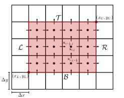
Figure 2: A staggered grid spatial discretization. The $x$-velocity component $u$ is solved for at locations depicted with horizontal arrows. The $y$-velocity component $v$ is solved for at locations depicted with vertical arrows. The pressure $p$ is solved for at locations depicted with a solid black dots. The corners $(x_{L},y_{L})$ and $(x_{U},y_{U})$ define the control volume $V_{\text{CV}}(t)$, which is shaded in red. The dashed line represents $S_{\text{CV}}(t)=\partial V_{\text{CV}}(t)$ = ${\mathcal{L}}\cup\mathcal{T}\cup{\mathcal{R}}\cup\mathcal{B}$.

3.2 Lagrange multiplier method

The hydrodynamic force and torque on an immersed body can also be computed in an extrinsic manner from force/torque balance laws. Specifically, for an immersed body occupying volume $V_{b}(t)$, the force and torque balance laws read as

$$\frac{{\rm d}}{{\rm d}t}\int_{V_{b}(t)}\rho\;\bm{\mathrm{U}}\,\mathrm{dV} =\bm{\mathrm{\mathcal{F}}}+\int_{V_{b}(t)}\bm{\mathrm{F}}\,\mathrm{dV},$$ (20)

$$\frac{{\rm d}}{{\rm d}t}\int_{V_{b}(t)}\rho\;\bm{\mathrm{R}}\wedge\bm{\mathrm{U}}\,\mathrm{dV} =\bm{\mathrm{\mathcal{M}}}+\int_{V_{b}(t)}\bm{\mathrm{R}}\wedge\bm{\mathrm{F}}\,\mathrm{dV},$$ (21)

in which $\bm{\mathrm{R}}=\bm{\mathrm{X}}-\bm{\mathrm{X}}_{0}$ is the radius vector from reference point $\bm{\mathrm{X}}_{0}$ to Lagrangian node position $\bm{\mathrm{X}}$, and $\bm{\mathrm{F}}$ is the Lagrange multiplier imposing rigidity constraint as defined in Eq. (3). Note that for the IB method, the net hydrodynamic force $\bm{\mathrm{\mathcal{F}}}$ and torque $\bm{\mathrm{\mathcal{M}}}$ on the body can be readily evaluated in the Lagrangian frame as a part of the solution process without computing any extra terms. We have used this approach in a previous work [13]. We will compare results obtained from both moving CV and LM method in Sec. 5.

3.3 Equivalence of the two methods

Although Eqs. (16) and (20) look different, we now show that the use of (regularized) delta functions in the IB method make them equivalent expressions. To prove this, consider a single body in the domain $\Omega$, occupying a region of space $V_{b}(t)\subset\Omega$. Let $\bm{\mathrm{F}}(\bm{\mathrm{s}},t)$ denote the Lagrange multiplier field defined on Lagrangian nodes, and $\bm{\mathrm{f}}(\bm{\mathrm{x}},t)$ denote its Eulerian counterpart. Here, $\bm{\mathrm{s}}\in U$ and $U\subset\mathbb{R}^{d}$. With continuous and Peskin’s discrete delta functions, the following identity holds

$$\int_{\Omega}\bm{\mathrm{f}}(\bm{\mathrm{x}},t)\,{\mathrm{d}}\bm{\mathrm{x}} =\int_{\Omega}\left[\int_{U\subset\Omega}\bm{\mathrm{F}}(\bm{\mathrm{s}},t)\,\delta(\bm{\mathrm{x}}-\bm{\mathrm{X}}(\bm{\mathrm{s}},t))\,{\mathrm{d}}\bm{\mathrm{s}}\right]\,{\mathrm{d}}\bm{\mathrm{x}}$$

$$=\int_{U\subset\Omega}\left[\int_{\Omega}\bm{\mathrm{F}}(\bm{\mathrm{s}},t)\,\delta(\bm{\mathrm{x}}-\bm{\mathrm{X}}(\bm{\mathrm{s}},t))\,{\mathrm{d}}\bm{\mathrm{x}}\right]\,{\mathrm{d}}\bm{\mathrm{s}}$$

$$=\int_{U\subset\Omega}\bm{\mathrm{F}}(\bm{\mathrm{s}},t)\left[\int_{\Omega}\delta(\bm{\mathrm{x}}-\bm{\mathrm{X}}(\bm{\mathrm{s}},t))\,{\mathrm{d}}\bm{\mathrm{x}}\right]{\mathrm{d}}\bm{\mathrm{s}}$$

$$=\int_{U}\bm{\mathrm{F}}(\bm{\mathrm{s}},t)\,{\mathrm{d}}\bm{\mathrm{s}}.$$ (22)

The above expression is the equivalence of Lagrangian and Eulerian force densities and is a well known result [5, 36]. Starting with the momentum Eq. (1) in Eulerian form

$$\rho\frac{\partial\bm{\mathrm{u}}}{\partial t}+\rho\nabla\cdot\mbox{}(\bm{\mathrm{u}}\bm{\mathrm{u}})=\nabla\cdot\mbox{}(-p\bm{\mathrm{I}}+\bm{\mathrm{T}})+\bm{\mathrm{f}},$$ (23)

and integrating it over $V_{\text{CV}}(t)$, we obtain

$$\int_{V_{\text{CV}}(t)}\rho\frac{\partial\bm{\mathrm{u}}}{\partial t}\,\mathrm{dV}+\int_{V_{\text{CV}}(t)}\rho\nabla\cdot\mbox{}(\bm{\mathrm{u}}\bm{\mathrm{u}})\,\mathrm{dV}=\int_{V_{\text{CV}}(t)}\nabla\cdot\mbox{}\left[-p\bm{\mathrm{I}}+\bm{\mathrm{T}}\right]\,\mathrm{dV}+\int_{V_{\text{CV}}(t)}\bm{\mathrm{f}}\,\mathrm{dV}.$$

Applying the divergence theorem to terms with $\nabla\cdot\mbox{}$, and using Eq. (22) we obtain

$$\int_{V_{\text{CV}}(t)}\bm{\mathrm{f}}\,\mathrm{dV}=\int_{V_{b}(t)}\bm{\mathrm{F}}\,\mathrm{dV}=\int_{V_{\text{CV}}(t)}\rho\frac{\partial\bm{\mathrm{u}}}{\partial t}\,\mathrm{dV}-\int_{S_{\text{CV}}(t)}\bm{\mathrm{n}}\cdot\left[-p\bm{\mathrm{I}}-\bm{\mathrm{u}}\rho\bm{\mathrm{u}}+\bm{\mathrm{T}}\right]\,\mathrm{dS}.$$ (24)

Using the above expression for $\int_{V_{b}(t)}\bm{\mathrm{F}}\,\mathrm{dV}$ with Eq. (20) we get force expression (16). Similarly, one can prove the equivalence of torque expressions (19) and (21) by noting that $\bm{\mathrm{r}}\wedge\nabla\cdot\mbox{}\bm{\mathrm{S}}=\nabla\cdot\mbox{}(\bm{\mathrm{r}}\wedge\bm{\mathrm{S}})$ for any symmetric tensor satisfying $\bm{\mathrm{S}}=\bm{\mathrm{S}}^{T}$.

When multiple bodies exist in the domain, however, there is a subtle difference in the LM and moving CV expressions. The LM expressions in the form of Eqs. (20) and (21) are restricted to individual bodies; therefore in the presence of multiple bodies, $\bm{\mathrm{\mathcal{F}}}$ and $\bm{\mathrm{\mathcal{M}}}$ can be computed separately for each body. For the moving CV method, care must be taken to restrict the control volume to a particular body, i.e. it should not enclose other bodies in its vicinity. Otherwise, $\bm{\mathrm{\mathcal{F}}}$ and $\bm{\mathrm{\mathcal{M}}}$ will contain contribution from multiple bodies. We explore this subtlety with the moving CV method by taking flow past two stationary cylinders in Sec. 5.1.3, and drafting-kissing-tumbling of two sedimenting cylinders in Sec. 5.5. For an AMR framework, the boundary of a control volume can span multiple refinement levels. When velocity is reconstructed from old hierarchy to new, there is generally no guarantee that momentum is conserved because of the inter-level velocity interpolation. This can lead to jumps in $\bm{\mathrm{\mathcal{F}}}$ and $\bm{\mathrm{\mathcal{M}}}$ because of the time derivative terms. Eqs. (20) and (21) are restricted to $V_{b}(t)$, which generally lies on the finest grid level. Therefore, one can expect force and torque calculations to be relatively insensitive to velocity reconstruction operations, which mostly requires intra-level interpolation. We explore this issue with translating plate example in Sec. 5.3.2.

4 Software implementation

We use the IBAMR library [48] to implement the moving control volume method in this work for our numerical tests. IBAMR has built-in support for direct forcing and fully constrained IB methods, among other variants of the IB method. IBAMR relies on SAMRAI [49, 50] for Cartesian grid management and the AMR framework. Solver support in IBAMR is provided by PETSc library [51, 52, 53].

5 Results

5.1 Flow past cylinder

In this section we validate our moving control volume method and Lagrange multiplier method for computing hydrodynamic forces and torques on immersed bodies.

5.1.1 Stationary cylinder

We first consider the flow past a stationary circular cylinder. The cylinder has diameter $D=1$ and is placed in a flow with far-field velocity $\bm{\mathrm{U}}_{\infty}=(U_{\infty},V_{\infty})=(1,0)$. The computational domain is a rectangular channel taken to be of size $18D\times 12D$, with the center of the cylinder placed at $(x,y)=(0,0)$. The domain is discretized by a uniform Cartesian mesh of size $900\times 600$. The aerodynamic drag coefficient $C_{D}=\bm{\mathrm{\mathcal{F}}}\cdot\bm{\mathrm{e}}_{x}/(\rho D\|\bm{\mathrm{U}}_{\infty}\|^{2}/2)$ is calculated numerically in two different ways: via Eq. (16) and via integrating Lagrange multipliers enforcing the rigidity constraint on the cylinder (Eq. (20)). The control volume is taken to be $[-D,1.5D]\times[-D,D]$ and does not move from its initial location. Note that in the case where both the body and the control volume are stationary, Eqs. (15) and (16) equivalent and give the same numerical solution. The density is set to $\rho=1$ and the Reynolds number of the flow is $\text{Re}=\rho U_{\infty}D/\mu=550$. This problem has been studied numerically by Bergmann and Iollo [34] and by Ploumhans and Winckelmans [54]. The temporal behavior of $C_{D}$ matches well with the previous studies [34, 54].

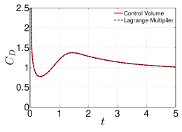
Figure 3: Comparison of the drag coefficient for flow past a cylinder at $\text{Re}=550$ measured in two different ways. (—, red): Control volume using Eq. (16); (---, black): Lagrange multiplier using Eq. (20).

5.1.2 Translating cylinder

Next, we consider the case of a circular cylinder translating with prescribed motion. The parameters used in this case are identical to those of the flow past a stationary cylinder case, except now $\bm{\mathrm{U}}_{\infty}=(U_{\infty},V_{\infty})=(0,0)$. The cylinder is dragged with speed $\bm{\mathrm{U}}_{\text{b}}=(U_{\text{b}},V_{\text{b}})=(-1,0)$. The aerodynamic drag coefficient is computed as $C_{D}=\bm{\mathrm{\mathcal{F}}}\cdot\bm{\mathrm{e}}_{x}/(\rho D\|\bm{\mathrm{U}}_{\text{b}}\|^{2}/2)$. The control volume is initially set to $[-D,1.5D]\times[-D,D]$ and translates to the left every few time steps to ensure that it always contains the cylinder. The density is set to $\rho=1$ and the Reynolds number is $\text{Re}=\rho U_{\text{b}}D/\mu=550$. Periodic boundary conditions are used on all faces of the computational domain. This problem was also studied numerically by Bergmann and Iollo [34].

Fig. 4 shows the time evolution of $C_{D}$ calculated in three different ways, via Eqs. (15) and (16) , and by integrating Lagrange multipliers. The present control volume method matches well with the Lagrange multiplier approach. However, spurious jumps in drag coefficient are seen for the original control volume method outlined by Noca. These spurious oscillations are also present in the computation done by Bergmann and Iollo [34]. We remark that the oscillations seen by Bergmann and Iollo [34] are quantitatively different than the ones presented here in Fig. 4 for comparison, although both use Eq. (15) to compute hydrodynamic force. This can be attributed to differences in the numerical method used to impose constraint: we use a constraint-based immersed boundary method whereas Bergmann and Iollo use a Brinkman penalization method.

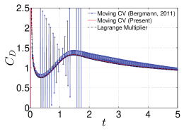
Figure 4: Comparison of the drag coefficient a translating cylinder at $\text{Re}=550$ measured in three different ways. $\bullet$: Control volume using Eq. (15); —: Control volume using Eq. (16); ---: Lagrange multiplier. Note that LM and present moving CV curves are on top of each other.

5.1.3 Two stationary cylinders

To study the effect of control volume size in the presence of multiple bodies, we consider the case of two stationary circular cylinders each with $D=1$ and placed in a flow with far-field velocity $\bm{\mathrm{U}}_{\infty}=(U_{\infty},V_{\infty})=(1,0)$. The bottom and top cylinders are centered about position $(x,y)=(0,-2D)$ and $(x,y)=(0,2D)$, respectively within a rectangular channel of size $18D\times 12D$. The domain is discretized by a uniform Cartesian mesh of size $900\times 600$ and the Reynolds number is $\text{Re}=\rho U_{\infty}D/\mu=550$ for each cylinder. The density of the fluid is set to $\rho=1$.

Four different (but symmetric) control volume configurations are considered:

1. Two disjoint CVs located at $[-D,D]\times[-3D,-D]$ and $[-D,D]\times[D,3D]$.

2. Two CVs located at $[-D,D]\times[-3D,D]$ and $[-D,D]\times[-D,3D]$ that slightly overlap, but do not intersect the other cylinder.

3. Two CVs located at $[-D,D]\times[-3D,2D]$ and $[-D,D]\times[-2D,3D]$, where each CV holds one full cylinder and half of the second cylinder.

4. Two CVs located at $[-D,D]\times[-3D,2.7D]$ and $[-D,D]\times[-2.7D,3D]$, where each CV contains both cylinders.

Fig. 5 shows flow visualizations for the four different CV configurations. Fig. 6 shows the drag coefficient over time for each of the four configurations. In the case where the CVs do not overlap (Figs. 5(a) and  6(a)), or when they overlap but do not enclose multiple bodies either partially or fully (Figs. 5(b) and  6(b)) the drag coefficients calculated for the top and bottom cylinders are close to the drag coefficient calculated for a single cylinder considered in Section 5.1.1.

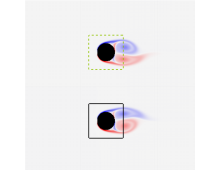
(a) No overlapping

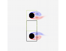
(b) Slightly overlapping

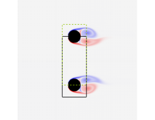
(c) CVs contain $1.5$ cylinders

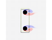
(d) CVs contain both cylinders

Figure 5: Vorticity generated by a circular cylinder at $t=5$ for $\text{Re}=550$: 5(a) two disjoint control volumes; 5(b) two slightly overlapping control volumes; 5(c) each control volume contains one and a half cylinders; 5(d) each control volume contains both cylinders. All figures are plotted for vorticity between $-20$ and $20$.

The effect of resizing the control volumes to partially or fully contain other objects is seen in the hydrodynamic drag force measurement. In the case where each CV contains one and a half cylinders (Figs. 5(c) and 6(c)), the drag coefficient deviates significantly from the drag coefficient calculated for a single cylinder. Rather, the computed force is the drag on a combined full and a half cylinder contained within the CV, which is approximately $1.5$ times the drag on a single cylinder. In the case where each CV contains both cylinders (Figs. 5(d) and 6(d)), the measured $C_{D}$ in each control volume is approximately twice the $C_{D}$ measured on a single cylinder. Therefore, in presence of multiple bodies in the domain, care must be taken to restrict the CV to an individual body.

(a) No overlapping

(b) Slightly overlapping

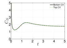
(c) CVs contain $1.5$ cylinders

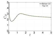
(d) CVs contain both cylinders

Figure 6: Temporal evolution of drag coefficient for $\text{Re}=550$: 6(a) two disjoint control volumes; 6(b) two slightly overlapping control volumes; 6(c) one and a half cylinders; 6(d) two full cylinders. —: Bottom CV; --- (green): Top CV.

5.2 Oscillating cylinder

In this section we consider cases from previous studies, some of which have reported spurious force oscillations in hydrodynamic drag and lift forces with IB methods. We do not observe such spurious force oscillations using LM and CV methods within an immersed boundary framework.

5.2.1 In-line oscillation

We consider an in-line oscillation of a circular cylinder in a quiescent flow as done in Dütsch et al. [55] and Lee et al. [29]. The cylinder has a diameter $D=1$ and is placed in a domain of size $[-16D,16D]\times[-8D,8D]$ with zero velocity prescribed on all boundaries of the domain. The initial center of mass of the cylinder is placed at $(0,0)$ and its velocity is set to $\bm{\mathrm{U}}_{\text{b}}=\left(-U_{0}\cos(2\pi ft),0\right)$, in which $f$ is the frequency of oscillation. The Reynolds number of the flow is $\text{Re}=\rho U_{0}D/\mu=100$, and the Keulegan-Carpenter number is $\text{KC}=U_{0}/(fD)=5$. The time period of oscillation of the cylinder is given by $T=1/f$. The density of the fluid is set to be $\rho=1$. These parameters are chosen to match those reported in [29, 55].

Three levels of mesh refinement are used, with $n_{\text{ref}}=4$ between each level. The cylinder is embedded in the finest mesh level at all time instances. At the coarsest level, three different mesh sizes are used: $50\times 25$, $100\times 50$, and $200\times 100$, which corresponds to finest grid spacings of $\Delta x_{\textrm{min}}=\Delta y_{\textrm{min}}=0.04D$, $\Delta x_{\textrm{min}}=\Delta y_{\textrm{min}}=0.02D$, and $\Delta x_{\textrm{min}}=\Delta y_{\textrm{min}}=0.01D$, respectively. The computational time step size is chosen to be $\Delta t=0.005D/U_{0}$, matching that of Lee at al.  [29]. This time step size satisfies the convective CFL condition with $C=0.7$, which is found to be stable for all the mesh sizes considered here. A stationary control volume is placed at $[-4D,4D]\times[-2D,2D]$ in order to contain the entire cylinder at all time instances. The drag coefficient is computed as $C_{D}=\bm{\mathrm{\mathcal{F}}}\cdot\bm{\mathrm{e}}_{x}/(0.5\rho U_{0}^{2}D)$.

Fig. 7 shows the time evolution of drag coefficient for the oscillating cylinder. Both CV and LM approaches yield identical results. Even our coarse resolution results are in good agreement with the high resolution results of Lee et al. [29]. Moreover, Lee et al. conducted this case within an immersed boundary framework and observed large spurious force oscillations (see Fig. 14 in [29]) at coarse grid resolutions. They compute drag on the immersed body by evaluating pressure and velocity gradients within the body region $V_{b}(t)$. Only at fine grid resolutions, where the spatial gradients are more accurate, were they able to suppress the spurious force oscillations. Since we do not require spatial gradients of velocity and pressure within the body region $V_{b}(t)$ with our approach, we do not observe such spurious oscillations.

(a) Control Volume

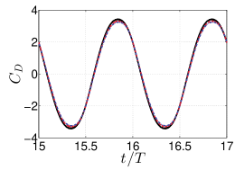
(b) Lagrange Multiplier

Figure 7: Temporal evolution of the drag coefficient of an oscillating cylinder at $\text{Re}=100$ measured by the 7(a) present control volume approach and 7(b) Lagrange multiplier approach. Here, (—, black): $\Delta x_{\textrm{min}}=\Delta y_{\textrm{min}}=0.04D$; (---, red): $\Delta x_{\textrm{min}}=\Delta y_{\textrm{min}}=0.02D$; (-$\cdot$-, blue): $\Delta x_{\textrm{min}}=\Delta y_{\textrm{min}}=0.01D$.

5.2.2 Cross-flow oscillation

Here we consider a cylinder oscillating in the transverse direction with an imposed cross-flow. The cylinder has a diameter $D=1$ and its initial center of mass is placed at $(x,y)=(0,0.2D)$. The cylinder is placed in a domain of size $[-5D,27D]\times[-8D,8D]$ and oscillates in the transverse direction with velocity $\bm{\mathrm{U}}_{\text{b}}=\left(0,-V_{0}\sin(2\pi f_{e}t)\right)$, where $f_{e}$ is the frequency of oscillation. An axial free-stream velocity $U_{\infty}$ is set at the inlet, top, and bottom faces of the computational domain. The transverse traction components are set to zero on the top and bottom boundaries, and the axial and transverse tractions are set to zero at the outflow boundary.

The density of the fluid is set to $\rho=1$ and the Reynolds number based on the free-stream velocity is $\text{Re}=\rho U_{\infty}D/\mu=185$. Letting $f_{0}=0.193U_{\infty}/D$ be the natural shedding frequency for a stationary cylinder, we set $f_{e}/f_{0}=1$. The maximum oscillation velocity of the cylinder is taken to be $0.159V_{0}/(f_{e}D)=0.2$. This case is considered in Lee et al. [29] and Guilmineau and Queutey [56]. A stationary CV is placed at $[-D,D]\times[-2D,2D]$, which contains the cylinder at all time instances (see Fig. 8).

The domain is discretized with three different uniform meshes of sizes $400\times 192$, $800\times 384$, and $1600\times 768$, which corresponds to grid spacings of $\Delta x=\Delta y=0.08D$, $\Delta x=\Delta y=0.04D$, and $\Delta x=\Delta y=0.02D$, respectively. A constant time step size of $\Delta t=0.005D/U_{\infty}$ is used for all the computations, matching that of Lee at al.  [29]. The time step size satisfies the convective CFL condition with $C=0.7$, which is found to be stable for all the mesh sizes considered here. Fig. 9 shows the time evolution of drag coefficient $C_{D}=\bm{\mathrm{\mathcal{F}}}\cdot\bm{\mathrm{e}}_{x}/(0.5\rho U_{\infty}^{2}D)$. Again, both the CV and LM approach produce identical results and do not incur spurious force oscillations even at coarse resolutions as observed by Lee et al. (see Fig. 16 in [29]).

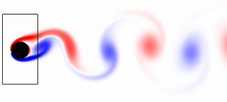
Figure 8: Vorticity generated by an oscillating cylinder in a cross-flow at $tU_{\infty}/D=100$ for $\text{Re}=185$. The plotted vorticity is between $-5$ and $5$.

(a) Control Volume

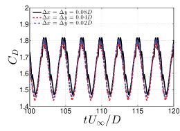
(b) Lagrange Multiplier

Figure 9: Temporal evolution of drag coefficient measured by the 9(a) present control volume approach and 9(b) Lagrange multiplier approach. Here, (—, black): $\Delta x=\Delta y=0.08D$; (---, red): $\Delta x=\Delta y=0.04D$; (-$\cdot$-, blue): $\Delta x=\Delta y=0.02D$.

5.2.3 Rotational oscillation

As a last example of this section, we consider the case of a cylinder undergoing a rotational oscillation about its center of mass in a quiescent flow. The diameter of the cylinder is taken to be $D=1$ and is placed in a domain of size $[-20D,20D]\times[-20D,20D]$, with zero velocity prescribed on all computational boundaries. The initial center of mass of the cylinder is placed at $(x,y)=(0,0)$ and it rotates about its center with a velocity $\omega_{b}=A_{m}\sin(2\pi ft)$, in which $f$ is the frequency of oscillation and $T=1/f$ is the time period of oscillation. The density of the fluid is set to be $\rho=1$. The Reynolds number of the flow is $\text{Re}=\rho U_{m}D/\mu=300$, in which $U_{m}=A_{m}D/2$. The cylinder rotates with frequency $f=0.1$ and has maximum angular velocity $A_{m}=10fD$. These parameters are chosen to match Borazjani et al. [57].

The time step size is chosen to be $\Delta t=1\times 10^{-4}T$ and the grid is discretized by a two level mesh, which consists of a coarse mesh of size $512\times 512$, and an embedded fine mesh with refinement ratio $n_{\text{ref}}=4$. The minimum grid spacing at the finest level is $\Delta x_{\textrm{min}}=\Delta y_{\textrm{min}}=0.0195D$. The structure remains on the finest grid level for at all time instances. A stationary control volume is placed at $[-1.01562D,1.01562D]^{2}$ and the torque coefficient is computed as $C_{T}=\bm{\mathrm{\mathcal{M}}}\cdot\bm{\mathrm{e}}_{z}/(0.5\rho U_{m}^{2}D)$. Fig. 10 shows the temporal evolution of $C_{T}$, which is in excellent agreement with sharp-interface CURVIB method results of Borazjani et al. [57].

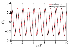
Figure 10: Comparison of the torque coefficient for a cylinder undergoing rotational oscillation at $\text{Re}=300$ measured in two different ways. Here, (—, red): Control volume using Eq. (19); (---, black): Lagrange multiplier using Eq. (21).

5.3 Moving plate

In this section we consider the effect of regridding on hydrodynamic force calculations using the control volume approach. In the context of an immersed body AMR framework, regridding occurs when the body has moved some distance, or when new flow features of interest have appeared in the computational domain that require additional mesh refinement to resolve them adequately. We consider a moving plate example to understand the jumps in the drag coefficient due to regridding, and to provide some strategies to mitigate them.

5.3.1 Moving plate on a uniform mesh

First we consider a single level domain case in two spatial dimensions. A finite plate of height $b=1$ is dragged perpendicular to itself with constant velocity $\bm{\mathrm{U}}_{\text{b}}=(U_{\text{b}},V_{\text{b}})=(-1,0)$ in an infinite fluid at rest. The plate is modeled as a thin line of points, separated by grid cell size distance in the transverse direction. The physical domain is a periodic box of dimension $32b\times 22b$ and the domain is discretized by a uniform Cartesian grid of size $1024\times 1024$. The initial location of the control volume is $[-2b,2b]\times[-b,b]$, and it moves with an arbitrary speed to enclose the plate at all time instances. The density of the fluid is set to be $\rho=1$. The Reynolds number of the flow is $\text{Re}=\rho U_{\text{b}}b/\mu=20$. The drag coefficient is calculated as $C_{D}=\bm{\mathrm{\mathcal{F}}}\cdot\bm{\mathrm{e}}_{x}/(\rho U_{\text{b}}^{2}b/2)$. An asymptotic solution $C_{D}\approx 2.09$ was derived by Dennis et al. [58], and this problem was also studied numerically by Bhalla et al. [13].

Fig. 11 shows the time evolution of drag coefficient for the moving plate. We see that the numerical solution obtained by the moving CV computation matches well with the asymptotic value derived in [58] and does not contains any spurious force oscillations or jumps.

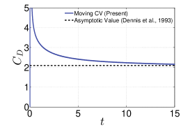
Figure 11: Comparison of the drag coefficient for a translating plate at $\text{Re}=20$ measured by the present moving control volume approach (—, blue); ---: asymptotic value from Dennis et al. [58].

5.3.2 Moving plate on an adaptive mesh

Next, we consider the same moving plate example but with locally refined grids. The domain is discretized by a coarse grid of size $256\times 256$. A more refined mesh immediately surrounds the plate with refinement ratio $n_{\text{ref}}=4$, giving the finest level an equivalent grid size of $1024\times 1024$. The mesh is adaptive in the sense that it selectively refines in areas with large velocity gradients and where the immersed body is located in the domain. Apart from the locally refined grids, we use the same parameters of Sec. 5.3.1 for this case.

Three different control volumes are used. First, the CV is set initially to $[-2b,2b]\times[-1.03125b,1.03125b]$ and it translates to the right along with the plate. In this configuration, the CV spans multiple levels of the grid hierarchy. Fig. 12 shows the measured drag coefficient over time. Again, $C_{D}$ evolves towards the asymptotic value derived in [58]. However, there are small jumps in $C_{D}$ over time, which are absent from the uniform mesh case of Sec. 5.3.1. These jumps can be attributed to the mesh hierarchy regridding to follow the moving plate or due to the moving CV itself. To rule out the possibility of jumps due to the motion of control volume, we consider a second CV configuration in which the CV is held stationary all times. The stationary CV again spans multiple grid levels and is big enough to contain the moving plate at all time instances. Fig. 13 shows the CV configuration and measured drag coefficient over time for this CV $=[-2b,-1.03125b]\times[20b,1.03125b]$. The jumps in $C_{D}$ are again observed. In our third configuration, we limit the moving CV on the finest grid level. The CV configuration and $C_{D}$ temporal profile is shown in Fig. 14. The initial location of this control volume is $[-b,0.625b]\times[-1.03125b,1.03125b]$.

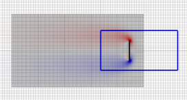
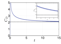
Figure 12: 12 Vorticity generated by a moving flat plate at $t=7.5$ for $\text{Re}=20$. The moving control volume spanning both the coarsest and finest grid level is shown in blue. The plotted vorticity is between $-7.5$ and $7.5$. 12 Temporal evolution of drag coefficient measured by the present moving control volume approach (—, blue); ---: asymptotic value from Dennis et al. [58].

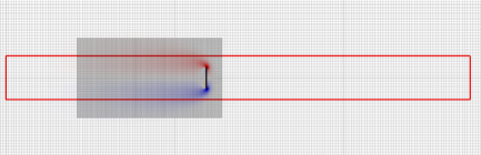
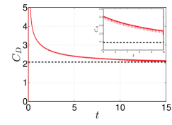
Figure 13: 12 Vorticity generated by a moving flat plate at $t=7.5$ for $\text{Re}=20$. The stationary control volume spanning both the coarsest and finest grid level is shown in red. The plotted vorticity is between $-7.5$ and $7.5$. 13 Temporal evolution of drag coefficient measured by the present control volume approach (—, red); ---: asymptotic value from Dennis et al. [58]

From Fig. 14, we note that the jumps due to regridding can be substantially mitigated if the moving CV is restricted to the finest mesh level. The CV translates to the right along with the plate, but remains on the finest mesh level throughout the simulation. There are no longer jumps in the computed drag values for $t\leq 10$.

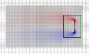
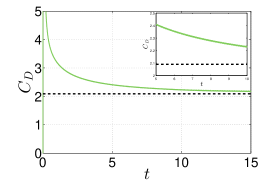
Figure 14: 14 Vorticity generated by a translating flat plate at $t=7.5$ for $\text{Re}=20$. The moving control volume spanning both the coarsest and finest grid level is shown in green. The plotted vorticity is between $-7.5$ and $7.5$. 14 Temporal evolution of drag coefficient measured by the present moving control volume approach (—, green); ---: asymptotic value from Dennis et al. [58].

The jumps in the hydrodynamic forces due to regridding occur due to velocity reconstruction following a regridding operation. A common velocity reconstruction strategy employed in an AMR framework is to first interpolate velocities from the coarser level to the new fine level, and then directly copy velocities from the old fine level in the spatial regions where old and new fine levels intersect. We refer readers to Griffith et al. [36] for details. When we restrict the moving CV to the finest grid level, we reduce errors in momentum change due to velocity reconstruction from coarse to fine level interpolation. The contribution of $\bm{\mathrm{u}}^{n}$ in the time derivative term in Eqs. (16) and (19) can be evaluated either before or after regridding. In our empirical tests, we have observed that evaluating the time derivative term after regridding helps in mitigating the jumps even further (comparison data not shown). In all our results shown above, we evaluate the contribution from $\bm{\mathrm{u}}^{n}$ after regridding, i.e, using the old velocity at the new hierarchy configuration.

5.4 Swimming eel

In this section we demonstrate that the moving control volume approach can be used to determine the hydrodynamic forces and torques on a free-swimming body. We consider a two-dimensional undulating eel geometry, which is adapted from [2, 13]. The eel’s reference frame is aligned with the $x$-axis and in this refrence frame the lateral displacement along $0\leq x\leq L$ over its projected length $L$ is given by

$$y(x,t)=0.125\frac{x+0.03125}{1.03125}\sin\left[2\pi(x-t/T)\right].$$ (25)

A backwards-traveling wave of the above form having a time period $T$ causes the eel to self-propel. The swimmer is taken to have a projected length $L=1$, and time period $T=1$. The Reynolds number based on $V_{\textrm{max}}=0.785L/T$, the maximum undulation velocity at the tail tip, is $\text{Re}=\rho V_{\textrm{max}}L/\mu=5609$. The undulations travel in the positive $x$-direction, thereby propelling the eel in the negative $x$-direction. The density of the fluid is taken to be $\rho=1$.

The eel’s total velocity $\bm{\mathrm{U}}_{\text{b}}=\bm{\mathrm{U}}_{\text{r}}+\bm{\mathrm{W}}_{\text{r}}\wedge\bm{\mathrm{R}}+\bm{\mathrm{U}}_{\text{k}}$ in the Lagrangian frame is given by the following components: its rigid linear $\bm{\mathrm{U}}_{\text{r}}$ and angular $\bm{\mathrm{W}}_{\text{r}}$ center of mass velocities and its deformational velocity $\bm{\mathrm{U}}_{\text{k}}$, which we assume to have zero net linear and angular momentum. The self-propulsion velocities are obtained using conservation of linear and angular momentum in the body domain $V_{b}(t)$

$$M_{\text{b}}\bm{\mathrm{U}}_{\text{r}}^{n+1} =\int_{V_{b}(t)}\rho\;\left(\bm{\mathrm{\mathcal{J}}}_{h}[\bm{\mathrm{X}}^{n+\frac{1}{2}}]\,\tilde{\bm{\mathrm{u}}}^{n+1}\right)\,\mathrm{dV},$$ (26)

$$\bm{\mathrm{I}}_{\text{b}}\bm{\mathrm{W}}_{\text{r}}^{n+1} =\int_{V_{b}(t)}\rho\;\bm{\mathrm{R}}^{n+\frac{1}{2}}\wedge\left(\bm{\mathrm{\mathcal{J}}}_{h}[\bm{\mathrm{X}}^{n+\frac{1}{2}}]\,\tilde{\bm{\mathrm{u}}}^{n+1}\right)\,\mathrm{dV},$$ (27)

in which $M_{\text{b}}$ and $\bm{\mathrm{I}}_{\text{b}}$ are the mass and moment of inertia tensor of the body, respectively. Having obtained these rigid body velocities, the body velocity at time $t^{n+1}$ required in Eq. (8) is obtained as $\bm{\mathrm{U}}_{\text{b}}^{n+1}=\bm{\mathrm{U}}_{\text{r}}^{n+1}+\bm{\mathrm{W}}_{\text{r}}^{n+1}\wedge\bm{\mathrm{R}}^{n+\frac{1}{2}}+\bm{\mathrm{U}}_{\text{k}}^{n+1}$, in which $\bm{\mathrm{R}}^{n+\frac{1}{2}}=\bm{\mathrm{X}}^{n+\frac{1}{2}}-\bm{\mathrm{X}}^{n+\frac{1}{2}}_{0}$ is the radius vector from (an estimated) midstep center of mass $\bm{\mathrm{X}}_{0}^{n+\frac{1}{2}}$ to (an estimated) midstep Lagrangian node position $\bm{\mathrm{X}}^{n+\frac{1}{2}}$. We refer readers to [13] for more details.

The fully periodic domain is taken to be of size $8L\times 4L$ and is discretized with a three-level hierarchy of Cartesian grids. The size of the coarsest grid is $128\times 64$ grid cells and $n_{\text{ref}}=4$ is taken for subsequent finer grids. Hence, the finest grid, with spacing equivalent to that of a uniform mesh of size $2048\times 1024$, embeds the undulatory swimmer at all times. A time step size of $\Delta t=1\times 10^{-4}\;T$ is employed. The head of the swimmer is initially centered at $(x,y)=(0,0)$ and its body extends in the positive $x$-direction. The CV is initially located at $[-1.02L,1.0425L]\times[-0.7075L,0.73L]$, which encompasses the entire swimmer. The CV is allowed to span multiple grid levels. Whenever the eel’s center of mass translates a distance $\Delta x$, the CV moves with velocity $\bm{\mathrm{u}}_{S}=(-\Delta x/\Delta t,0)$ in order to remain aligned with the grid lines. Fig. 15 shows the vortical structures generated by the eel at four separate time instances, along with the locations of the moving control volume.

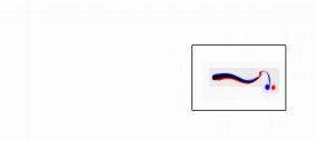
(a) $t/T=1$

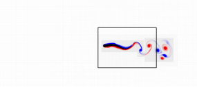
(b) $t/T=3$

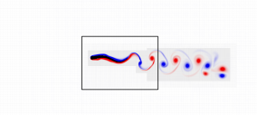
(c) $t/T=5$

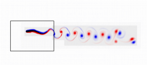
(d) $t/T=7$

Figure 15: Vorticity generated by the two-dimensional eel model at $\text{Re}=5609$, along with the moving CV location at four different time instances on an adaptive mesh hierarchy. All figures are plotted for vorticity between $-10$ and $10$.

Fig. 16 shows the time evolution of axial ($U_{r}=\bm{\mathrm{U}}_{\text{r}}\cdot\bm{\mathrm{e}}_{x}$) and lateral ($V_{r}=\bm{\mathrm{U}}_{\text{r}}\cdot\bm{\mathrm{e}}_{y}$) swimming velocities, along with the rotational velocity $W^{z}_{r}=\bm{\mathrm{W}}_{\text{r}}\cdot\bm{\mathrm{e}}_{z}$. The eel is shown to travel in the $-\bm{\mathrm{e}}_{x}$ direction, eventually reaching a steady state speed. The angular velocity oscillates about a zero mean value, while the lateral velocity has small non-zero mean due to initial transients. Fig. 16 shows the time evolution of net axial ($\mathcal{F}_{x}=\bm{\mathrm{\mathcal{F}}}\cdot\bm{\mathrm{e}}_{x}$) and lateral ($\mathcal{F}_{y}=\bm{\mathrm{\mathcal{F}}}\cdot\bm{\mathrm{e}}_{y}$) forces acting on the eel’s body, along with the net torque $\mathcal{M}_{z}=\bm{\mathrm{\mathcal{M}}}\cdot\bm{\mathrm{e}}_{z}$, which is measured from the eel’s center of mass. The forces and torque are computed using the moving CV approach, although identical estimates are obtained from the LM approach (data not shown). Both $\bm{\mathrm{\mathcal{F}}}$ and $\bm{\mathrm{\mathcal{M}}}$ oscillate about a mean value of zero, which is expected during free-swimming as there are no external forces and torques applied on the swimmer.

For an object initially at rest in a periodic and quiescent fluid, the net linear momentum over the entire computational domain should remain zero [13], i.e., $\bm{\mathrm{\mathcal{P}}}(t)=\int_{\Omega}\rho\bm{\mathrm{u}}\,\mathrm{dV}=\bm{\mathrm{0}}$. Similarly, the net angular momentum of the system should also remain zero at all times, i.e., $\bm{\mathrm{\mathcal{L}}}(t)=\int_{\Omega}\rho\bm{\mathrm{r}}\wedge\bm{\mathrm{u}}\,\mathrm{dV}=\bm{\mathrm{0}}$. In other words, all of the momentum generated due to the eel’s vortex shedding should be redistributed to the eel’s translational and rotational motion. Moreover, the change in linear momentum of the body should be equal to the net force on the body during free-swimming. Hence, the net force on the body should be given by $\bm{\mathrm{\mathcal{F}}}(t)=\frac{{\rm d}}{{\rm d}t}\int_{V_{b}}\rho\bm{\mathrm{u}}\,\mathrm{dV}$, implying that

$$\bm{\mathrm{\mathcal{I}}}(t)=-\int_{V_{\text{CV}}(t)}\rho\frac{\partial\bm{\mathrm{u}}}{\partial t}\,\mathrm{dV}+\oint_{S_{\text{CV}}(t)}\bm{\mathrm{n}}\cdot\left[-p\bm{\mathrm{I}}-\bm{\mathrm{u}}\rho\bm{\mathrm{u}}+\bm{\mathrm{T}}\right]\,\mathrm{dS}=\bm{\mathrm{0}}.$$ (28)

The above statement also implies the conservation of linear momentum for the control volume. Eq. (28) also implies that the sum of the Langrange multipliers enforcing the rigidity constraint within $V_{b}(t)$ is zero during free-swimming (see Eq. (24)). Fig. 16 shows the temporal evolution of ${\mathcal{P}}_{x}=\bm{\mathrm{\mathcal{P}}}\cdot\bm{\mathrm{e}}_{x}$, ${\mathcal{P}}_{y}=\bm{\mathrm{\mathcal{P}}}\cdot\bm{\mathrm{e}}_{y}$, $\mathcal{I}_{x}=\bm{\mathrm{\mathcal{I}}}\cdot\bm{\mathrm{e}}_{x}$, and $\mathcal{I}_{y}=\bm{\mathrm{\mathcal{I}}}\cdot\bm{\mathrm{e}}_{y}$; it is indeed seen that these quantities are nearly zero for all time instances. The slight increase in ${\mathcal{P}}_{x}$ is attributed to spatial and temporal discretization errors, whereas the jumps in $\mathcal{I}_{x}$ correspond to time steps at which regridding occurs. Similar observations are made for angular momentum conservation for the entire system (data not shown here).

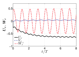
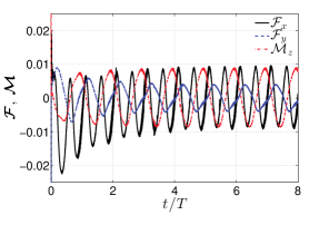
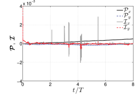
Figure 16: 16 Temporal evolution of (—, black) axial $U_{r}$ & (---, blue) lateral $V_{r}$ swimming velocity, and (-$\cdot$-, red) rotational $W_{r}^{z}$ velocity of the eel calculated by Eqs. (26) and (27). 16 Temporal evolution of net (—, black) axial $\mathcal{F}_{x}$ & (---, blue) lateral $\mathcal{F}_{y}$ forces, and (-$\cdot$-, red) net torque $\mathcal{M}_{z}$ on the body of the eel measured by the present moving control volume approach. 16 Temporal evolution of (—, black) axial ${\mathcal{P}}_{x}$ and (---, blue) lateral ${\mathcal{P}}_{y}$ momentum of the entire fluid domain. Temporal evolution of change in linear momentum within the control volume: (—, gray) $\mathcal{I}_{x}$ and (---, red) $\mathcal{I}_{y}$.

5.5 Drafting, kissing, and tumbling

In this section we simulate the dynamic interactions between two sedimenting cylindrical particles and use the moving control volume and Lagrange multiplier approaches to determine the hydrodynamic forces. The cylinders are identically shaped with diameter $D=0.2$ cm and are placed in a domain of size $[-5D,5D]\times$ [0, 40D], with zero velocity prescribed on the left and right boundaries, and with axial and transverse tractions set to zero at the top and bottom boundaries. The density and viscosity of the fluid are set to $\rho=1.0$ g/cm³ and $\mu=0.01$ g/(cm $\cdot$ s), respectively. Each particle is subject to a gravitational body force $\bm{\mathrm{F}}^{g}=-(\rho_{s}-\rho)gV_{p}\bm{\mathrm{e}}_{y}$, where $g=980$ cm/s² is the gravitational constant, $\rho_{s}=1.01\rho$ is the density of the solid, and $V_{p}=\pi(D/2)^{2}$ is the volume of each particle. This is realized through an Eulerian body force $\bm{\mathrm{f}}^{g}$ added to the right-hand side the momentum Eq. (1), which is nonzero only in the particle domains. Similar to the free-swimming eel case, the particles’ translational and rotational velocities are obtained via Eqs. (26) and (27).

The domain is discretized with a two-level hierarchy of Cartesian grids. The size of the coarsest grid is $64\times 256$ grid cells and $n_{\text{ref}}=4$ is taken for subsequent finer grids. Hence, the finest grid, with spacing equivalent to that of a uniform mesh of size $256\times 1024$, embeds each particle at all times. The minimum grid spacing on the finest level is $\Delta x_{\textrm{min}}=\Delta y_{\textrm{min}}=0.0390625D$. A time step size of $\Delta t=5\times 10^{-4}$ s is used. Particle $1$ is placed with initial center of mass $\bm{\mathrm{x}}_{1}=(X_{p},Y_{p})=(-0.005D,36D)$, while particle $2$ is placed below particle $1$ with initial center of mass location at $\bm{\mathrm{x}}_{2}=(X_{p},Y_{p})=(0,34D)$. Under these conditions, the two particles start to accelerate downwards due to gravity. Particle $1$ travels through a low pressure wake created by the leading particle $2$, which causes particle $1$ to fall faster; this stage is called drafting. Eventually, particle $1$ catches up to and nearly contacts particle $2$, a process termed as kissing in literature. This kissing stage is unstable and eventually the particles are left to tumble separately. The parameters here are chosen to match with previous numerical studies on drafting, kissing, and tumbling done by Feng et al. [59], Jafari et al. [60], and Wang et al. [61].

Artificial repulsive forces are added to avoid numerical issues due to overlapping particles. The functional form of this force on particle $i$ due to particle $j$ is given by

$$\bm{\mathrm{F}}_{ij}^{P}=\begin{cases}0,&\|\bm{\mathrm{x}}_{i}-\bm{\mathrm{x}}_{j}\|>R_{i}+R_{j}+\zeta\textrm{ or }i=j\\ \frac{c_{ij}}{\epsilon_{P}}\left(\frac{\|\bm{\mathrm{x}}_{i}-\bm{\mathrm{x}}_{j}\|-R_{i}-R_{j}-\zeta}{\zeta}\right)^{2}\left(\frac{\bm{\mathrm{x}}_{i}-\bm{\mathrm{x}}_{j}}{\|\bm{\mathrm{x}}_{i}-\bm{\mathrm{x}}_{j}\|}\right),&\|\bm{\mathrm{x}}_{i}-\bm{\mathrm{x}}_{j}\|\leq R_{i}+R_{j}+\zeta\end{cases}$$ (29)

in which $R_{i}=R_{j}=R$ is the radius of both particles, $c_{ij}=\rho\pi R^{2}g$ is a force scale parameter, $\epsilon_{P}=2.0$ g cm/s² is a stiffness parameters for collisions, and $\zeta=\Delta y_{\textrm{min}}$ is a mesh threshold parameter indicating how far away the two particles need to be in order to feel particle-particle interaction force. This particular repulsive force was used by Feng et al. [59]. No repulsive force between the particle and the wall are used for the case considered here. Similar to the gravitational force, the particle interaction force is realized through an Eulerian body force $\bm{\mathrm{f}}_{P}$ added to the right-hand side of the momentum Eq. (1), which is nonzero only in the particle domains.

The strategy for placing the control volume for this example is different than the previous examples. Rather than setting the CV in motion with some prescribed velocity to enclose the body, the CVs are chosen to surround each cylinder based on its center of mass location: $[X_{p}-5\Delta x_{\textrm{min}},X_{p}+5\Delta x_{\textrm{min}}]\times[Y_{p}-5\Delta y_{\textrm{min}},Y_{p}+5\Delta y_{\textrm{min}}]$. This means that when the particles are close to each other during the kissing stage, each CV contains the second body partially, leading to inaccurate force measurements. This is a limitation of using simple rectangular control volumes. Fig. 17 shows the vortical structures generated by the two particles at four separate time instances, along with the locations of the moving control volumes.

(a) $t=0.5$

(b) $t=1.5$

(c) $t=2.0$

(d) $t=3.0$

Figure 17: Vorticity generated by two-dimensional drafting, kissing, and tumbling of two cylindrical particles, along with the moving CV location at four different time instances on an adaptive mesh hierarchy. All figures are plotted for vorticity between $-30$ and $30$.

The expression for hydrodynamic force based on the Lagrange multiplier method needs to be modified to account for the presence of additional body forces in the solid region (additional to the Lagrange multiplier constraint forces). These forces need to be added to the right-hand side of Eq. (20), yielding

$$\bm{\mathrm{\mathcal{F}}}_{i}=\frac{{\rm d}}{{\rm d}t}\int_{V_{b}^{i}(t)}\rho\;\bm{\mathrm{U}}_{i}\,\mathrm{dV}-\int_{V_{b}^{i}(t)}(\bm{\mathrm{F}}_{i}+\bm{\mathrm{F}}_{i}^{g}+\bm{\mathrm{F}}_{ij}^{P})\,\mathrm{dV},$$ (30)

in which $\bm{\mathrm{\mathcal{F}}}_{i}$, $\bm{\mathrm{U}}_{i}$, $\bm{\mathrm{F}}_{i}$, $\bm{\mathrm{F}}_{i}^{g}$and $V_{b}^{i}(t)$ are the net hydrodynamic force, center of mass velocity, Lagrange multiplier force, gravitational force, and domain of particle $i$, respectively. The expression for hydrodynamic force based on control volume analysis remains unchanged in the presence of the additional body forces in the solid region, and Eq. (16) remains valid in this scenario.

Figs. 18 and 18 show the time evolution of the centers of mass $(X_{p},Y_{p})$ of both particles. Particle $1$ gradually approaches particle $2$ up until near $t=2.5$ s when the particles kiss and eventually separate. Upon separation, both particles over time reach a terminal velocity. This temporal behavior matches well with the results of Jafari et al. [60]. Figs. 18 and 18 show the time evolution of net axial ($\mathcal{F}_{x}=\bm{\mathrm{\mathcal{F}}}\cdot\bm{\mathrm{e}}_{x}$) and lateral ($\mathcal{F}_{y}=\bm{\mathrm{\mathcal{F}}}\cdot\bm{\mathrm{e}}_{y}$) forces acting on each particle, calculated using both the control volume and Lagrange multiplier approaches. Between $t=1$ s and $t=2.5$ s, the particles are close to each other and it is not possible to create rectangular CVs that contain only a single particle (see insets in Figs. 17(b) and  17(c)). Hence, the CV force calculations during this time period are inaccurate. However, the forces calculated by the LM method remain accurate at all times. Outside of this time period, both the CV and LM approaches are in excellent agreement. Eventually, the net hydrodynamic force on each particle is $-\bm{\mathrm{F}}^{g}$, indicating a terminal velocity has been achieved.

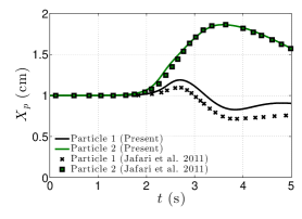
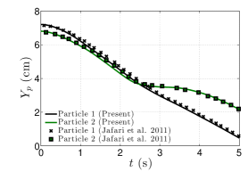
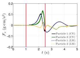
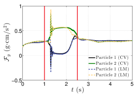
Figure 18: 18 Temporal evolution of the $x$ coordinate of center of mass $X_{p}$ for (—, black) particle $1$ & (—, green) particle $2$. 18 Temporal evolution of the $y$ coordinate of center of mass $Y_{p}$ for (—, black) particle $1$ & (—, green) particle $2$. Center of mass data from Jafari et al. [60] for ($\times$, black) particle $1$ & ($\blacksquare$, green) particle $2$. 18 Temporal evolution of net $\mathcal{F}_{x}$ via the moving control volume approach on (—, black) particle $1$ & (—, green) particle $2$. Temporal evolution of net $\mathcal{F}_{x}$ via the Lagrange multiplier approach approach on (---, blue) particle $1$ & (---, yellow) particle $2$. 18 Temporal evolution of net $\mathcal{F}_{y}$ via the moving control volume approach on (—, black) particle $1$ & (—, green) particle $2$. Temporal evolution of net $\mathcal{F}_{y}$ via the Lagrange multiplier approach approach on (---, blue) particle $1$ & (---, yellow) particle $2$. The time period between the two red lines indicates inaccurate CV force measurements since each rectangular CV contains multiple bodies.

5.6 Stokes flow

In the previous sections, we considered finite Reynolds number cases simulated using a direct forcing IB method in which Lagrange multipliers were approximated in the body domain. Here we consider a fully constrained IB method in which we compute Lagrange multipliers exactly. We consider Stokes flow examples here, although the fully constrained method also work equally well at finite Reynolds numbers as shown in [16].

For steady Stokes flow in the absence of inertia ($\rho=0$), the momentum equation reads as

$$-\nabla p(\bm{\mathrm{x}})+\mu\nabla^{2}\bm{\mathrm{u}}(\bm{\mathrm{x}})+\bm{\mathrm{f}}(\bm{\mathrm{x}})=\bm{\mathrm{0}}.$$ (31)

Since Eq. (31) is a steady state problem, it cannot be solved numerically with the split fluid-structure solver described in [13]. Rather, the discretized system of Eqs. (11)-(13) are solved by the monolithic fluid-structure solver described in [16] to obtain a numerical solution to the constrained Stokes system. The rigidity constraint is enforced on the surface of the body, and the body is discretized only by surface nodes and not by a volumetric mesh. This is because enforcing the rigidity constraint on the surface also imposes rigid body motion inside the body for Stokes flow. Setting the inertial terms to zero in Eqs. $\eqref{eq_OurForce}$ and $\eqref{eq_OurTorque}$ yield

$$\bm{\mathrm{\mathcal{F}}} =\oint_{S_{\text{CV}}}\bm{\mathrm{n}}\cdot\left[-p\bm{\mathrm{I}}+\bm{\mathrm{T}}\right]\,\mathrm{dS},$$ (32)

$$\bm{\mathrm{\mathcal{M}}} =\oint_{S_{\text{CV}}}[\bm{\mathrm{r}}\wedge(-p\;\bm{\mathrm{n}}+\bm{\mathrm{n}}\cdot\bm{\mathrm{T}})\;]\,\mathrm{dS}.$$ (33)

Hence, the net hydrodynamic force and torque on an object in Stokes flow is simply the pressure and viscous fluxes through the control surface. For the LM method, the Lagrange multiplier force density $\bm{\mathrm{F}}(\bm{\mathrm{X}})$ is computed (exactly) on body surface $\bm{\mathrm{X}}\in S_{b}$, and the net force and torque is given by

$$\bm{\mathrm{\mathcal{F}}} =-\oint_{S_{b}}\bm{\mathrm{F}}(\bm{\mathrm{X}})\,\mathrm{dS},$$ (34)

$$\bm{\mathrm{\mathcal{M}}} =-\oint_{S_{b}}\bm{\mathrm{R}}\wedge\bm{\mathrm{F}}(\bm{\mathrm{X}})\,\mathrm{dS}.$$ (35)

5.6.1 Flow between two concentric shells

We first consider the case of two concentric shells, which was studied numerically by Kallemov et al. [16]. The inner and outer shell have geometric radii $R_{1}^{g}=1.807885$ and $R_{2}^{g}=4R_{1}^{g}$, respectively. The computational domain is a cube of size $[0,L]^{3}=[0,4.15R_{2}^{g}]^{3}$, which is discretized by a uniform grid of size $60^{3}$. The center of both shells is placed at $(x,y,z)=(L/2,L/2,L/2)$. Uniform velocity $\bm{\mathrm{u}}=(1,0,0)$ is prescribed on each wall of the computational domain, and the inner and outer shell are set to have rigid–body velocity $(U_{1},V_{1},W_{1})=(0,0,0)$ and $(U_{2},V_{2},W_{2})=(1,0,0)$, respectively. The inner shell is discretized with $42$ surface markers while the outer shell is discretized with $642$ surface markers to ensure that the markers are about $2$ grid cells apart. The viscosity is set to $\mu=1$.

Each spherical shell has an effective hydrodynamic radius $R^{h}$ due to the immersed boundary kernel used to discretize the delta-function [62]. For the 6-point kernel considered by Kallemov et al., it was found that $R_{1}^{h}=1.22R_{1}^{g}$ and $R_{2}^{h}=0.96R_{2}^{g}$ for the numerical parameters chosen here [16]. It was also found that as both the Eulerian and Lagrangian meshes are refined, $R^{h}/R^{g}\rightarrow 1$. These hydrodynamic radii can be used in the analytical expression for the drag on the inner sphere [63], given by

$$\bm{\mathrm{\mathcal{F}}}_{\textrm{exact}}\cdot\bm{\mathrm{e}}_{x}=-6\pi\mu R_{1}^{h}U_{2}K,$$ (36)

in which $K=(1-\lambda^{5})/\alpha$, $\alpha=1-9\lambda/4+5\lambda^{3}/2-9\lambda^{5}/4+\lambda^{6}$ and $\lambda=R_{1}^{h}/R_{2}^{h}$.

Depending on the control volume size, the drag on either the inner shell, or on both shells can be obtained. First, a CV of dimension $[L/2-1.659R_{1}^{g},L/2+1.659R_{1}^{g}]^{3}$ is chosen to surround the inner shell, but to exclude the outer shell. Next, a CV of dimension $[L/2-1.383R_{2}^{g},L/2+1.383R_{2}^{g}]$ is chosen to include both inner and outer shells. Fig. 19 shows the configuration of the concentric shells/spheres and the two control volumes.

Table 1 shows the drag measurements from the analytical expression, from integrating surface Lagrange multipliers, and from the control volume analysis. The middle column shows that all three methods are in agreement for the drag on the inner shell. Moreover, the last column shows that the combined drag on both inner and outer shells is the same when computed from Lagrange multipliers and control volume analysis.

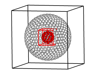
Figure 19: Surface nodes on the inner shell (red) and outer shell (gray) for Stokes flow between concentric spheres. Location of a control volume containing only the inner shell (red) and containing both the inner and outer shell (black).

Table 1: Comparison of force measurements for Stokes flow around two concentric spheres.

Method	$|\bm{\mathrm{\mathcal{F}}}\cdot\bm{\mathrm{e}}_{x}|$ (Inner)	$|\bm{\mathrm{\mathcal{F}}}\cdot\bm{\mathrm{e}}_{x}|$ (Inner & Outer)
Analytical Eq. (36)	115.409	N/A
Lagrange multiplier Eq. (34)	114.297	17.350
Control volume Eq. (32)	114.298	17.350

5.6.2 Single rotating shell

Next, we consider a single shell rotating in a bounded domain with no exterior flow. The shell is taken to be the same as the inner sphere in the previous example, with geometric radius $R_{1}^{g}=1.807885$ in a computational domain of size $[0,L]^{3}=[0,16.6R_{1}^{g}]^{3}$. There is no outer shell in this example. The center of the shell is placed at the centroid of the cube $(x,y,z)=(L/2,L/2,L/2)$ and $\bm{\mathrm{u}}=(0,0,0)$ is set at all computational boundaries. Periodic boundary conditions were also used and yielded nearly identical torque measurements (data not shown). The viscosity is set to $\mu=1$. The shell rotates about a diameter with angular velocity $\bm{\mathrm{\omega}}=(0,1,0)$. In an unbounded flow at rest, Faxén’s law states that the torque on the sphere by the fluid is

$$\bm{\mathrm{\mathcal{M}}}=-8\pi\mu(R_{1}^{h})^{3}\bm{\mathrm{\omega}},$$ (37)

in which the hydrodynamic radius of the sphere $R_{1}^{h}$ is used [63]. Although the domain in the numerical method is bounded, we still get decent agreement between our numerical results and Eq. (37).

A CV of dimension $[L/2-1.659R_{1}^{g},L/2+1.659R_{1}^{g}]^{3}$ is chosen to surround the shell. Three different grid sizes are used to discretize the domain: $60^{3}$, $120^{3}$, and $240^{3}$, which corresponds to $42$, $162$, and $642$ surface markers on the shell respectively (to ensure that the markers are approximately 2 grid cells apart).

Table 2 shows the torque measurements $\bm{\mathrm{\mathcal{M}}}\cdot\bm{\mathrm{e}}_{y}$ from the analytical expression, from integrating the moments of surface Lagrange multipliers, and from the control volume analysis, for the three different grid resolutions. As expected, the LM and CV measured torque do not match exactly with the analytical expression (presumably because of finite domain effects). However, the LM and CV torque values are in excellent agreement with each other.

Table 2: Comparison of torque measurements $\bm{\mathrm{\mathcal{M}}}\cdot\bm{\mathrm{e}}_{y}$ for Stokes flow around single rotating sphere.

Grid size	Number of markers	$R_{1}^{h}/R_{1}^{g}$ [16]	Analytical Eq. (37)	LM Eq. (35)	CV Eq. (33)
$60^{3}$	42	1.22	-269.669	-236.474	-236.474
$120^{3}$	162	1.09	-192.323	-183.662	-183.662
$240^{3}$	642	1.04	-167.052	-164.446	-164.446

Conclusions

In the present study we presented a moving control volume (CV) approach to compute the net hydrodynamic forces and torques on a moving body immersed in a fluid. This approach does not require evaluation of (possibly) discontinuous spatial velocity or pressure gradients within or on the surface of the immersed body. The analytical expressions for forces and torques were modified from those initially presented in [32], and this modification has been shown to eliminate spurious jumps in drag [34]. Our implementation treats the control volume as a rectangular box whose boundary is forced to remain on grid lines, which greatly simplifies the evaluation of surface integrals.

The approach is shown to accurately compute the forces and torques on a wide array of fluid-structure interaction problems, including flow past stationary and moving objects, Stokes flow, and high Reynolds number free-swimming. Spurious momentum gain or loss due to adaptive mesh refinement can produce jumps in the computed forces in the CV approach, although forcing the CV to remain on the finest grid level can ameliorate this issue.

We also show the equivalence between the Lagrange multiplier (LM) approach and the CV approach. The main advantage of the CV approach over the LM approach is that it is applicable to situations where explicit Lagrange multipliers are not available, for example, in the embedded boundary/cut-cell approach to FSI.

The control volume approach implemented here assumes a no-slip boundary condition on the fluid-structure interface. However, a generalization for transpiration boundary conditions can be derived as well (see Eq. (44)). Use of such a boundary condition would required richer geometric information and data structures to evaluate surface quantities of the immersed body. Finally, our approach can be easily extended to cases where additional body forces are present in the momentum equation.

Appendix A Derivation of the new hydrodynamic force expression

Here we present a detailed derivation of Eq. (16) from Eq. (15). The ultimate goal is to obtain an expression for hydrodynamic force which involves integral contributions from a single CV rather than two time-lagged CVs. The Reynolds transport theorem (RTT) [30, 31] gives an expression for the time derivative of an arbitrary quantity $\bm{\mathrm{q}}(\bm{\mathrm{x}},t)$ on a time dependent region $\Omega(t)$

$$\frac{{\rm d}}{{\rm d}t}\int_{\Omega(t)}\bm{\mathrm{q}}\,\mathrm{dV}=\int_{\Omega(t)}\frac{\partial\bm{\mathrm{q}}}{\partial t}\,\mathrm{dV}+\oint_{\partial\Omega(t)}(\bm{\mathrm{n}}\cdot\bm{\mathrm{u}}_{S})\bm{\mathrm{q}}\,\mathrm{dS},$$ (38)

in which $\bm{\mathrm{u}}_{S}$ is the velocity and $\bm{\mathrm{n}}$ is the outward pointing unit normal vector of the boundary $\partial\Omega(t)$. Applying the RTT to Eq. (15) yields the expression

$$\bm{\mathrm{\mathcal{F}}}(t) =-\int_{V(t)}\rho\frac{\partial\bm{\mathrm{u}}}{\partial t}\,\mathrm{dV}-\oint_{\partial V(t)}(\bm{\mathrm{n}}\cdot\bm{\mathrm{u}}_{S})\rho\bm{\mathrm{u}}\,\mathrm{dS}$$

$$+\oint_{S_{\text{CV}}(t)}\bm{\mathrm{n}}\cdot\left[-p\bm{\mathrm{I}}-(\bm{\mathrm{u}}-\bm{\mathrm{u}}_{S})\rho\bm{\mathrm{u}}+\bm{\mathrm{T}}\right]\,\mathrm{dS}-\oint_{S_{b}(t)}\bm{\mathrm{n}}\cdot(\bm{\mathrm{u}}-\bm{\mathrm{u}}_{S})\rho\bm{\mathrm{u}}\,\mathrm{dS}.$$ (39)

Recall that $V(t)=V_{\text{CV}}(t)\setminus V_{b}(t)$, where $V_{\text{CV}}(t)$ is the entire control volume and contains the body domain $V_{b}(t)$; $S_{\text{CV}}(t)=\partial V_{\text{CV}}(t)$ is the boundary of the CV, and $S_{b}(t)=\partial V_{b}(t)$. Hence, $\partial V(t)=S_{\text{CV}}(t)\cup S_{b}(t)$. and the second integral can be split into two boundary integrals

$$\bm{\mathrm{\mathcal{F}}}(t)= -\int_{V(t)}\rho\frac{\partial\bm{\mathrm{u}}}{\partial t}\,\mathrm{dV}$$

$$-\oint_{S_{\text{CV}}(t)}(\bm{\mathrm{n}}\cdot\bm{\mathrm{u}}_{S})\rho\bm{\mathrm{u}}\,\mathrm{dS}+\oint_{S_{\text{CV}}(t)}\bm{\mathrm{n}}\cdot\left[-p\bm{\mathrm{I}}-(\bm{\mathrm{u}}-\bm{\mathrm{u}}_{S})\rho\bm{\mathrm{u}}+\bm{\mathrm{T}}\right]\,\mathrm{dS}$$ (40)

$$-\oint_{S_{b}(t)}(\bm{\mathrm{n}}\cdot\bm{\mathrm{u}}_{S})\rho\bm{\mathrm{u}}\,\mathrm{dS}-\oint_{S_{b}(t)}\bm{\mathrm{n}}\cdot(\bm{\mathrm{u}}-\bm{\mathrm{u}}_{S})\rho\bm{\mathrm{u}}\,\mathrm{dS},$$

which can be simplified to obtain

$$\bm{\mathrm{\mathcal{F}}}(t)=-\int_{V(t)}\rho\frac{\partial\bm{\mathrm{u}}}{\partial t}\,\mathrm{dV}+\oint_{S_{\text{CV}}(t)}\bm{\mathrm{n}}\cdot\left[-p\bm{\mathrm{I}}-\bm{\mathrm{u}}\rho\bm{\mathrm{u}}+\bm{\mathrm{T}}\right]\,\mathrm{dS}-\oint_{S_{b}(t)}\bm{\mathrm{n}}\cdot(\bm{\mathrm{u}}\rho\bm{\mathrm{u}})\,\mathrm{dS}.$$ (41)

Recall that in Eq. (41), the unit normal vector points outward on $S_{\text{CV}}(t)$ and inward on $S_{b}(t)$ since the integral is considered with respect to the boundary of $V(t)$. Next, notice that by definition $V_{\text{CV}}(t)=V(t)\cup V_{b}(t)$ is the union of disjoint regions. Hence, the integral over $V(t)$ can be split into $\int_{V(t)}\bm{\mathrm{q}}\,\mathrm{dV}=\left(\int_{V_{\text{CV}}(t)}-\int_{V_{b}(t)}\right)\bm{\mathrm{q}}\,\mathrm{dV}$. Applying the split to Eq. (41) yields

$$\bm{\mathrm{\mathcal{F}}}(t)=-\int_{V_{\text{CV}}(t)}\rho\frac{\partial\bm{\mathrm{u}}}{\partial t}\,\mathrm{dV}+\int_{V_{b}(t)}\rho\frac{\partial\bm{\mathrm{u}}}{\partial t}\,\mathrm{dV}+\oint_{S_{\text{CV}}(t)}\bm{\mathrm{n}}\cdot\left[-p\bm{\mathrm{I}}-\bm{\mathrm{u}}\rho\bm{\mathrm{u}}+\bm{\mathrm{T}}\right]\,\mathrm{dS}-\oint_{S_{b}(t)}\bm{\mathrm{n}}\cdot(\bm{\mathrm{u}}\rho\bm{\mathrm{u}})\,\mathrm{dS}.$$ (42)

Finally, we can apply the Reynolds transport theorem (Eq.  (38)) to the integral over $V_{b}(t)$ above. Letting $\bm{\mathrm{N}}$ be the outward pointing unit normal vector to $S_{b}(t)$, we obtain

$$\bm{\mathrm{\mathcal{F}}}(t)= -\int_{V_{\text{CV}}(t)}\rho\frac{\partial\bm{\mathrm{u}}}{\partial t}\,\mathrm{dV}+\frac{{\rm d}}{{\rm d}t}\int_{V_{b}(t)}\rho\bm{\mathrm{u}}\,\mathrm{dV}$$

$$+\oint_{S_{\text{CV}}(t)}\bm{\mathrm{n}}\cdot\left[-p\bm{\mathrm{I}}-\bm{\mathrm{u}}\rho\bm{\mathrm{u}}+\bm{\mathrm{T}}\right]\,\mathrm{dS}$$ (43)

$$-\oint_{S_{b}(t)}(\bm{\mathrm{N}}\cdot\bm{\mathrm{u}}_{S})\rho\bm{\mathrm{u}}\,\mathrm{dS}-\oint_{S_{b}(t)}\bm{\mathrm{n}}\cdot(\bm{\mathrm{u}}\rho\bm{\mathrm{u}})\,\mathrm{dS}.$$

Substituting the fact that $\bm{\mathrm{N}}=-\bm{\mathrm{n}}$ yields a general expression for the hydrodynamic force on an immersed body

$$\bm{\mathrm{\mathcal{F}}}(t)=-\int_{V_{\text{CV}}(t)}\rho\frac{\partial\bm{\mathrm{u}}}{\partial t}\,\mathrm{dV}+\frac{{\rm d}}{{\rm d}t}\int_{V_{b}(t)}\rho\bm{\mathrm{u}}\,\mathrm{dV}+\oint_{S_{\text{CV}}(t)}\bm{\mathrm{n}}\cdot\left[-p\bm{\mathrm{I}}-\bm{\mathrm{u}}\rho\bm{\mathrm{u}}+\bm{\mathrm{T}}\right]\,\mathrm{dS}-\oint_{S_{b}(t)}\bm{\mathrm{n}}\cdot(\bm{\mathrm{u}}\rho\bm{\mathrm{u}}-\bm{\mathrm{u}}_{S}\rho\bm{\mathrm{u}})\,\mathrm{dS}.$$ (44)

Eq. (44) can be further simplified if we assume no-slip boundary conditions at the fluid-structure interface by setting $\bm{\mathrm{u}}_{S}=\bm{\mathrm{u}}$, which gives

$$\bm{\mathrm{\mathcal{F}}}(t)=-\int_{V_{\text{CV}}(t)}\rho\frac{\partial\bm{\mathrm{u}}}{\partial t}\,\mathrm{dV}+\frac{{\rm d}}{{\rm d}t}\int_{V_{b}(t)}\rho\bm{\mathrm{u}}\,\mathrm{dV}+\oint_{S_{\text{CV}}(t)}\bm{\mathrm{n}}\cdot\left[-p\bm{\mathrm{I}}-\bm{\mathrm{u}}\rho\bm{\mathrm{u}}+\bm{\mathrm{T}}\right]\,\mathrm{dS}.$$ (45)

This is the net hydrodynamic force expression as written in Eq. (16).

Appendix B Derivation of the new hydrodynamic torque expression

Conservation of angular momentum for a material volume $V_{m}(t)$ (a volume that moves with the local fluid velocity) that shares its boundary with an arbitrary moving control volume $V(t)$ at time $t$ can be written as [30, 31]

$$\frac{d}{dt}\int_{V_{m}(t)}(\bm{\mathrm{r}}\wedge\rho\bm{\mathrm{u}})\,\mathrm{dV} =\oint_{\partial V_{m}(t)=\partial V(t)}\bm{\mathrm{r}}\wedge[\bm{\mathrm{n}}\cdot\Sigma]\,\mathrm{dS}$$

$$=\oint_{S_{\text{CV}}(t)}\bm{\mathrm{r}}\wedge[\bm{\mathrm{n}}\cdot\Sigma]\,\mathrm{dS}+\oint_{S_{b}(t)}\bm{\mathrm{r}}\wedge[\bm{\mathrm{n}}\cdot\Sigma]\,\mathrm{dS},$$ (46)

in which $\bm{\mathrm{r}}=\bm{\mathrm{x}}-\bm{\mathrm{x}}_{0}$, with $\bm{\mathrm{x}}_{0}$ as a reference point for computing torques, and $\Sigma=-p\bm{\mathrm{I}}+\bm{\mathrm{T}}$. Letting $\bm{\mathrm{\mathcal{M}}}(t)$ be the torque exerted by the fluid on the body and noticing that $\oint_{S_{b}(t)}\bm{\mathrm{r}}\wedge[\bm{\mathrm{n}}\cdot\Sigma]\,\mathrm{dS}=-\bm{\mathrm{\mathcal{M}}}(t)$, we have

$$\bm{\mathrm{\mathcal{M}}}(t)=-\frac{d}{dt}\int_{V_{m}(t)}(\bm{\mathrm{r}}\wedge\rho\bm{\mathrm{u}})\,\mathrm{dV}+\oint_{S_{\text{CV}}(t)}\bm{\mathrm{r}}\wedge[\bm{\mathrm{n}}\cdot\Sigma]\,\mathrm{dS}.$$ (47)

Using the RTT, the integral of an arbitrary quantity $\Phi$ over the material volume $V_{m}(t)$ can be related to integral over arbitrary volume $V(t)$ with surface velocity moving with $\bm{\mathrm{u}}_{S}$ as

$$\frac{d}{dt}\int_{V_{m}(t)}\Phi\,\mathrm{dV}=\frac{d}{dt}\int_{V(t)}\Phi\,\mathrm{dV}+\oint_{\partial V_{m}(t)=\partial V(t)}\bm{\mathrm{n}}\cdot(\bm{\mathrm{u}}-\bm{\mathrm{u}}_{S})\Phi\,\mathrm{dS}.$$ (48)

Using Eq. (48) with $\Phi=\bm{\mathrm{r}}\wedge\rho\bm{\mathrm{u}}$, the expression for torque becomes

$$\bm{\mathrm{\mathcal{M}}}(t) =-\frac{d}{dt}\int_{V(t)}(\bm{\mathrm{r}}\wedge\rho\bm{\mathrm{u}})\,\mathrm{dV}+\oint_{S_{\text{CV}}(t)}[\bm{\mathrm{r}}\wedge(-p\;\bm{\mathrm{n}}+\bm{\mathrm{n}}\cdot\bm{\mathrm{T}})-\bm{\mathrm{n}}\cdot(\bm{\mathrm{u}}-\bm{\mathrm{u}}_{S})(\bm{\mathrm{r}}\wedge\rho\bm{\mathrm{u}})]\,\mathrm{dS}$$

$$-\oint_{S_{b}(t)}\bm{\mathrm{n}}\cdot(\bm{\mathrm{u}}-\bm{\mathrm{u}}_{S})(\bm{\mathrm{r}}\wedge\rho\bm{\mathrm{u}})\,\mathrm{dS}.$$ (49)

Finally, by manipulating the term derivative term in Eq. (49) using the RTT we get an expression for torque on an immersed body as

$$\bm{\mathrm{\mathcal{M}}}(t)=-\int_{V_{\text{CV}}(t)}\rho\bm{\mathrm{r}}\wedge\frac{\partial\bm{\mathrm{u}}}{\partial t}\,\mathrm{dV}+\frac{d}{dt}\int_{V_{b}(t)}\rho(\bm{\mathrm{r}}\wedge\bm{\mathrm{u}})\,\mathrm{dV}+\oint_{S_{\text{CV}}(t)}[\bm{\mathrm{r}}\wedge(-p\;\bm{\mathrm{n}}+\bm{\mathrm{n}}\cdot\bm{\mathrm{T}})-(\bm{\mathrm{n}}\cdot\bm{\mathrm{u}})\rho(\bm{\mathrm{r}}\wedge\bm{\mathrm{u}})\;]\,\mathrm{dS}.$$ (50)

Appendix C Numerical discretization

Here we describe the discrete evaluation of Eqs. (16) and (19) to obtain the net hydrodynamic force and torque on an immersed body. For notational simplicity, we present the discretized equations in two spatial dimensions. An extension to three spatial dimensions is straightforward. A discrete grid covers the physical domain $\Omega$ with mesh spacing $\Delta x$ and $\Delta y$ in each direction. The position of each grid cell center is given by $\bm{\mathrm{x}}_{i,j}=\left(x_{i,j},y_{i,j}\right)$. For a given cell center, $\bm{\mathrm{x}}_{i-\frac{1}{2},j}$ denotes the physical location of the cell face that is half a grid space away from $\bm{\mathrm{x}}_{i,j}$ in the negative $x$-direction, i.e. $\bm{\mathrm{x}}_{i-\frac{1}{2},j}=\left(x_{i,j}-\frac{\Delta x}{2},y_{i,j}\right)$. Similarly $\bm{\mathrm{x}}_{i,j-\frac{1}{2}}$ denotes the physical location of the cell face that is half a grid cell away from $\bm{\mathrm{x}}_{i,j}$ in the negative $y$-direction, i.e. $\bm{\mathrm{x}}_{i,j-\frac{1}{2}}=\left(x_{i,j},y_{i,j}-\frac{\Delta y}{2}\right)$. The discrete approximations described here are also valid when adaptive mesh refinement is used, although volume weights need to be appropriately modified for different velocity components.

Let $t^{n}$ be the time at time step $n$. After stepping forward from time $t^{n}$ to $t^{n+1}=t^{n}+\Delta t$, a pressure solution is obtained at cell centers $p_{i,j}^{n+1}=p\left(\bm{\mathrm{x}}_{i,j},t^{n+1}\right)$, while velocity components are obtained at cell faces: $u_{i-\frac{1}{2},j}^{n+1}=u\left(\bm{\mathrm{x}}_{i-\frac{1}{2},j},t^{n+1}\right)$ and $v_{i,j-\frac{1}{2}}^{n+1}=v\left(\bm{\mathrm{x}}_{i,j-\frac{1}{2}},t^{n+1}\right)$. These are the only Eulerian quantities needed to evaluate the discrete approximations to Eqs. (16) and (19). Only rectangular control volumes are considered in the present work. A CV is described by its lower left and upper right corners: letting $(x_{L},y_{L})$ and $(x_{U},y_{U})$ denote the lower and upper corners respectively, the control volume is defined to be the Cartesian product of intervals $V_{\text{CV}}(t)=\left\{\bm{\mathrm{x}}\in\Omega\mid\bm{\mathrm{x}}\in[x_{L},x_{U}]\times[y_{L},y_{U}]\right\}$. Moreover, $S_{\text{CV}}(t)$ is forced to remain on grid lines and it not allowed to cross into the interior of grid cells. This greatly simplifies the required numerical approximations. Refer to Fig. 2 for a sketch of the control volume configuration over a staggered mesh discretization. Let the control volume and surface at a time instance $t^{n+1}$ be denoted by $V_{\text{CV}}^{n+1}=V_{\text{CV}}(t^{n+1})$ and $S_{\text{CV}}^{n+1}=S_{\text{CV}}(t^{n+1})$, respectively.

C.1 Discrete approximation to surface integrals

The control surface $S_{\text{CV}}^{n+1}$ is composed of four segments (eight faces in $3$D) denoted by $\mathcal{B}$, ${\mathcal{L}}$, $\mathcal{T}$, and ${\mathcal{R}}$ in Fig. 2. Consequently, computing surface normals on each of these segments is simple, e.g for the bottom segment $\mathcal{B}^{n+1}$, $\bm{\mathrm{n}}=-\bm{\mathrm{e}}_{y}$. The discretized surface integral of a quantity $\bm{\mathrm{\Phi}}$ over $S_{\text{CV}}^{n+1}$ is simply the sum over these four segments

$$\oint_{S_{\text{CV}}^{n+1}}\bm{\mathrm{n}}\cdot\bm{\mathrm{\Phi}}\,\mathrm{dS}=\oint_{{\mathcal{R}}^{n+1}}\bm{\mathrm{e}}_{x}\cdot\bm{\mathrm{\Phi}}\,\mathrm{dS}-\oint_{{\mathcal{L}}^{n+1}}\bm{\mathrm{e}}_{x}\cdot\bm{\mathrm{\Phi}}\,\mathrm{dS}+\oint_{\mathcal{T}^{n+1}}\bm{\mathrm{e}}_{y}\cdot\bm{\mathrm{\Phi}}\,\mathrm{dS}-\oint_{\mathcal{B}^{n+1}}\bm{\mathrm{e}}_{y}\cdot\bm{\mathrm{\Phi}}\,\mathrm{dS}.$$ (51)

Moreover, it is sufficient to show the discrete approximation to the surface integral over a single segment since the contribution from the other three segments are computed analogously. Over the bottom surface $\mathcal{B}$, the discretization of each term is given by

$$\oint_{\mathcal{B}}\bm{\mathrm{n}}\cdot\left(-p\bm{\mathrm{I}}\right)\,\mathrm{dS} =\oint_{\mathcal{B}}-\bm{\mathrm{e}}_{y}\left(-p\right)\,\mathrm{dS}$$

$$\approx\sum_{(i,j-\frac{1}{2})\in\mathcal{B}}-\bm{\mathrm{e}}_{y}\frac{-(p_{i,j}+p_{i,j-1})}{2}\Delta x,$$ (52)

$$\oint_{\mathcal{B}}\bm{\mathrm{n}}\cdot\left(-\bm{\mathrm{u}}\rho\bm{\mathrm{u}}\right)\,\mathrm{dS} =-\rho\oint_{\mathcal{B}}-v\left(u\bm{\mathrm{e}}_{x}+v\bm{\mathrm{e}}_{y}\right)\,\mathrm{dS}$$

$$\approx-\rho\sum_{(i,j-\frac{1}{2})\in\mathcal{B}}-v_{i,j-\frac{1}{2}}\left[\frac{u_{i-\frac{1}{2},j}+u_{i+\frac{1}{2},j}+u_{i-\frac{1}{2},j-1}+u_{i+\frac{1}{2},j-1}}{4}\bm{\mathrm{e}}_{x}+v_{i,j-\frac{1}{2}}\bm{\mathrm{e}}_{y}\right]\Delta x,$$ (53)

$$\oint_{\mathcal{B}}\bm{\mathrm{n}}\cdot\mu\left(\nabla\bm{\mathrm{u}}+\nabla\bm{\mathrm{u}}^{T}\right)\,\mathrm{dS} =\mu\oint_{\mathcal{B}}-\left[\left(\frac{\partial u}{\partial y}+\frac{\partial v}{\partial x}\right)\bm{\mathrm{e}}_{x}+2\frac{\partial v}{\partial y}\bm{\mathrm{e}}_{y}\right]\,\mathrm{dS}$$

$$\approx\mu\sum_{(i,j-\frac{1}{2})\in\mathcal{B}}-\left[\left(\frac{u_{i+\frac{1}{2},j}-u_{i+\frac{1}{2},j-1}+u_{i-\frac{1}{2},j}-u_{i-\frac{1}{2},j-1}}{2\Delta y}+\frac{v_{i+1,j-\frac{1}{2}}-v_{i-1,j-\frac{1}{2}}}{2\Delta x}\right)\bm{\mathrm{e}}_{x}\right]\Delta x$$

$$+\mu\sum_{(i,j-\frac{1}{2})\in\mathcal{B}}-\left[2\frac{v_{i,j+\frac{1}{2}}-v_{i,j-\frac{3}{2}}}{2\Delta y}\bm{\mathrm{e}}_{y}\right]\Delta x.$$ (54)

Fig. 20 shows a schematic of the pressure and velocity values required to evaluate Eqs. (52), (53), and (54). Evaluating the surface integral on $\mathcal{B}$ in the torque calculation about a point $\bm{\mathrm{x}}_{0}$ is done by computing $\bm{\mathrm{r}}_{i,j-\frac{1}{2}}=\bm{\mathrm{x}}_{i,j-\frac{1}{2}}-\bm{\mathrm{x}}_{0}$ and evaluating the cross product between $\bm{\mathrm{r}}_{i,j-\frac{1}{2}}$ and the integrand.

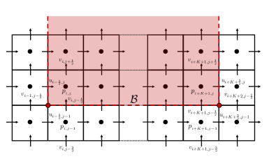
Figure 20: The velocity and pressure locations on the staggered–grid discretization required to evaluate the surface integral terms in the hydrodynamic force calculation on the bottom face of $S_{\text{CV}}$.

C.2 Change in control volume momentum

A discretization of the the time derivative term in Eq. (16) for the integral over $V_{\text{CV}}(t)$ at time step $n+1$ is given by

$$-\int_{V_{\text{CV}}^{n+1}}\rho\frac{\partial\bm{\mathrm{u}}}{\partial t}\,\mathrm{dV}\approx-\int_{V_{\text{CV}}^{n+1}}\rho\frac{\bm{\mathrm{u}}^{n+1}-\bm{\mathrm{u}}^{n}}{\Delta t}\,\mathrm{dV}=-\frac{1}{\Delta t}\int_{V_{\text{CV}}^{n+1}}\rho\bm{\mathrm{u}}^{n+1}\,\mathrm{dV}+\frac{1}{\Delta t}\int_{V_{\text{CV}}^{n+1}}\rho\bm{\mathrm{u}}^{n}\,\mathrm{dV},$$ (55)

where a discrete approximation to the total linear momentum within $V_{\text{CV}}^{n+1}$ can be written as

$$\int_{V_{\text{CV}}^{n+1}}\rho\bm{\mathrm{u}}\,\mathrm{dV}\approx\bm{\mathrm{e}}_{x}\sum_{(i-\frac{1}{2},j)\in V_{\text{CV}}^{n+1}}\rho u_{i-\frac{1}{2},j}\Delta V_{i-\frac{1}{2},j}+\bm{\mathrm{e}}_{y}\sum_{(i,j-\frac{1}{2})\in V_{\text{CV}}^{n+1}}\rho v_{i,j-\frac{1}{2}}\Delta V_{i,j-\frac{1}{2}}.$$ (56)

Here, $\Delta V=\frac{\Delta x\Delta y}{2}$ when either $(i-\frac{1}{2},j)\in S_{\text{CV}}^{n+1}$ or $(i,j-\frac{1}{2})\in S_{\text{CV}}^{n+1}$, and $\Delta V=\Delta x\Delta y$ otherwise, to ensure that $\sum_{(i-\frac{1}{2},j)}\Delta V_{i-\frac{1}{2},j}=\sum_{(i,j-\frac{1}{2})}\Delta V_{i,j-\frac{1}{2}}=\left|V_{\text{CV}}^{n+1}\right|$, the volume of the CV.

In the original hydrodynamic force formula Eq. (15) introduced by Noca [32], a discretization of the momentum term is given by

$$-\frac{{\rm d}}{{\rm d}t}\int_{V_{\text{CV}}^{n+1}}\rho\bm{\mathrm{u}}\,\mathrm{dV}\approx-\frac{1}{\Delta t}\int_{V_{\text{CV}}^{n+1}}\rho\bm{\mathrm{u}}^{n+1}\,\mathrm{dV}+\frac{1}{\Delta t}\int_{V_{\text{CV}}^{n}}\rho\bm{\mathrm{u}}^{n}\,\mathrm{dV}.$$ (57)

Notice that Eqs. (55) and (57) are nearly identical, although the former only requires an evaluation over a single CV, while the latter requires an evaluation over two time-lagged CVs.

The analogous term in the torque calculation Eq. (19) is discretized differently. Each $u$ velocity location $\bm{\mathrm{x}}_{i-\frac{1}{2},j}$ is looped over and an approximation to $v$ is computed. Then $\bm{\mathrm{r}}_{i-\frac{1}{2},j}=\bm{\mathrm{x}}_{i-\frac{1}{2}}-\bm{\mathrm{x}}_{0}$ is computed and used in the cross product. Mathematically, this is realized as

$$-\int_{V_{\text{CV}}^{n+1}}\rho\bm{\mathrm{r}}\wedge\frac{\partial\bm{\mathrm{u}}}{\partial t}\,\mathrm{dV}\approx-\frac{1}{\Delta t}\int_{V_{\text{CV}}^{n+1}}\rho\bm{\mathrm{r}}\wedge\bm{\mathrm{u}}^{n+1}\,\mathrm{dV}+\frac{1}{\Delta t}\int_{V_{\text{CV}}^{n+1}}\rho\bm{\mathrm{r}}\wedge\bm{\mathrm{u}}^{n}\,\mathrm{dV},$$ (58)

in which

$$\int_{V_{\text{CV}}^{n+1}}\rho\bm{\mathrm{r}}\wedge\bm{\mathrm{u}}\,\mathrm{dV}\approx\sum_{(i-\frac{1}{2},j)\in V_{\text{CV}}^{n+1}}\bm{\mathrm{r}}_{i-\frac{1}{2},j}\wedge\left[u_{i-\frac{1}{2},j}\bm{\mathrm{e}}_{x}+\frac{v_{i-1,j-\frac{1}{2}}+v_{i,j-\frac{1}{2}}+v_{i-1,j+\frac{1}{2}}+v_{i,j+\frac{1}{2}}}{4}\bm{\mathrm{e}}_{y}\right]\Delta V_{i-\frac{1}{2},j}.$$ (59)

C.3 Change in body momentum

The final term that needs to be discretely approximated is the change in momentum of the immersed body. This is presented as an integral of the body’s velocity over the region $V_{b}(t)\subset\Omega$ in an Eulerian reference frame. Since the body’s position and velocity are described in a Lagrangian reference frame over a region $I_{b}\subset U$, it is generally much easier to evaluate the Lagrangian form of this integral instead. Using the definition of $\delta(\bm{\mathrm{x}})$, it can be shown that the momentum over these two different reference frames are equivalent:

$$\int_{V_{b}}\rho\bm{\mathrm{u}}(\bm{\mathrm{x}},t){\mathrm{d}}\bm{\mathrm{x}}=\int_{I_{b}}\rho\bm{\mathrm{U}}(\bm{\mathrm{s}},t){\mathrm{d}}\bm{\mathrm{s}}.$$ (60)

Letting $\mathcal{G}^{n}$ denote the collection of discrete IB points corresponding to the region $I_{b}$ at time step $n$, the object’s momentum is obtained by

$$\bm{\mathrm{\mathcal{P}}}_{\text{b}}^{n}=\sum_{(l,m)\in\mathcal{G}^{n}}\rho\bm{\mathrm{U}}_{l,m}^{n}\Delta\bm{\mathrm{s}}_{l,m},$$ (61)

in which $\bm{\mathrm{U}}_{l,m}^{n}$ denotes the velocity of IB node $(l,m)$ at time step $n$, and $\Delta\bm{\mathrm{s}}_{l,m}$ denotes the discrete volume occupied by the node. The change in momentum required for the evaluation of hydrodynamic forces is then given by

$$\frac{{\rm d}}{{\rm d}t}\int_{I_{b}}\rho\bm{\mathrm{U}}(\bm{\mathrm{s}},t){\mathrm{d}}\bm{\mathrm{s}}\approx\frac{\bm{\mathrm{\mathcal{P}}}_{\text{b}}^{n+1}-\bm{\mathrm{\mathcal{P}}}_{\text{b}}^{n}}{\Delta t}.$$ (62)

The change in the body’s angular momentum for the torque calculation is done similarly.

Bibliography

Bibliography

- [1] H. H. Hu, N. A. Patankar, M. Zhu, Direct numerical simulations of fluid–solid systems using the arbitrary lagrangian–eulerian technique, J Comput Phys 169 (2) (2001) 427–462.
- [2] S. Kern, P. Koumoutsakos, Simulations of optimized anguilliform swimming, Journal of Experimental Biology 209 (24) (2006) 4841–4857.
- [3] R. Glowinski, T.-W. Pan, T. I. Hesla, D. D. Joseph, A distributed lagrange multiplier/fictitious domain method for particulate flows, Int J Multiphase Flow 25 (5) (1999) 755–794.
- [4] N. A. Patankar, P. Singh, D. D. Joseph, R. Glowinski, T.-W. Pan, A new formulation of the distributed Lagrange multiplier/fictitious domain method for particulate flows, Int J Multiphase Flow 26 (9) (2000) 1509–1524.
- [5] C. S. Peskin, The immersed boundary method, Acta Numer 11 (2002) 479–517.
- [6] C. S. Peskin, Flow patterns around heart valves: a numerical method, J Comput Phys 10 (2) (1972) 252–271.
- [7] E. P. Newren, A. L. Fogelson, R. D. Guy, R. M. Kirby, Unconditionally stable discretizations of the immersed boundary equations, J Comput Phys 222 (2) (2007) 702–719.
- [8] E. P. Newren, A. L. Fogelson, R. D. Guy, R. M. Kirby, A comparison of implicit solvers for the immersed boundary equations, Comput Meth Appl Mech Eng 197 (25–28) (2008) 2290–2304.
- [9] R. D. Guy, B. Philip, A multigrid method for a model of the implicit immersed boundary equations, Comm Comput Phys 12 (2) (2012) 378–400.
- [10] A. P. S. Bhalla, M. G. Knepley, M. F. Adams, R. D. Guy, B. E. Griffith, Scalable smoothing strategies for a geometric multigrid method for the immersed boundary equations, arXiv preprint arXiv:1612.02208.
- [11] Y. Mori, C. S. Peskin, Implicit second order immersed boundary methods with boundary mass, Comput Meth Appl Mech Eng 197 (25–28) (2008) 2049–2067.
- [12] M. Uhlmann, An immersed boundary method with direct forcing for the simulation of particulate flows, J Comput Phys 209 (2) (2005) 448–476.
-
[13]
A. P. S. Bhalla, R. Bale, B. E. Griffith, N. A. Patankar,
A
unified mathematical framework and an adaptive numerical method for
fluid-structure interaction with rigid, deforming, and elastic bodies, J
Comput Phys 250 (1) (2013) 446–476.
doi:10.1016/j.jcp.2013.04.033.
URL http://linkinghub.elsevier.com/retrieve/pii/S0021999113003173 - [14] A. P. S. Bhalla, R. Bale, B. E. Griffith, N. A. Patankar, Fully resolved immersed electrohydrodynamics for particle motion, electrolocation, and self-propulsion, J Comput Phys 256 (2014) 88–108.
- [15] K. Taira, T. Colonius, The immersed boundary method: A projection approach, J Comput Phys 225 (2) (2007) 2118–2137.
- [16] B. Kallemov, A. P. S. Bhalla, B. E. Griffith, A. Donev, An immersed boundary method for rigid bodies, Comm Appl Math Comput Sci 11 (1) (2016) 79–141.
- [17] F. Balboa Usabiaga, B. Kallemov, B. Delmotte, A. P. S. Bhalla, B. E. Griffith, A. Donev, Hydrodynamics of suspensions of passive and active rigid particles: a rigid multiblob approach, Communications in Applied Mathematics and Computational Science 11 (2) (2016) 217–296. doi:10.2140/camcos.2016.11.217.
- [18] H. D. Ceniceros, J. E. Fisher, A. M. Roma, Efficient solutions to robust, semi-implicit discretizations of the immersed boundary method, J Comput Phys 228 (19) (2009) 7137–7158.
- [19] L. Zhang, A. Gerstenberger, X. Wang, W. K. Liu, Immersed finite element method, Comput Meth Appl Mech Eng 193 (21–22) (2004) 2051–2067.
- [20] W. K. Liu, Y. Liu, D. Farrell, L. Zhang, X. S. Wang, Y. Fukui, N. Patankar, Y. Zhang, C. Bajaj, J. Lee, J. Hong, X. Chen, H. Hsu, Immersed finite element method and its applications to biological systems, Comput Meth Appl Mech Eng 195 (13–16) (2006) 1722–1749.
- [21] L. Heltai, F. Costanzo, Variational implementation of immersed finite element methods, Comput Meth Appl Mech Eng 229–232 (2012) 110–127.
- [22] B. E. Griffith, X. Luo, Hybrid finite difference/finite element immersed boundary method, International Journal for Numerical Methods in Biomedical Engineering.
- [23] M.-C. Lai, Z.-L. Li, A remark on jump conditions for the three-dimensional Navier-Stokes equations involving an immersed moving membrane, Appl Math Lett 14 (2) (2001) 149–154.
- [24] Z.-L. Li, M.-C. Lai, The immersed interface method for the Navier-Stokes equations with singular forces, J Comput Phys 171 (2) (2001) 822–842.
- [25] Y.-H. Tseng, J. H. Ferziger, A ghost-cell immersed boundary method for flow in complex geometry, J Comput Phys 192 (2) (2003) 593–623.
- [26] R. Mittal, H. Dong, M. Bozkurttas, F. Najjar, A. Vargas, A. von Loebbecke, A versatile sharp interface immersed boundary method for incompressible flows with complex boundaries, J Comput Phys 227 (10) (2008) 4825–4852.
- [27] H. Udaykumar, R. Mittal, P. Rampunggoon, A. Khanna, A sharp interface cartesian grid method for simulating flows with complex moving boundaries, J Comput Phys 174 (1) (2001) 345–380.
- [28] D. Trebotich, D. Graves, An adaptive finite volume method for the incompressible navier–stokes equations in complex geometries, Communications in Applied Mathematics and Computational Science 10 (1) (2015) 43–82.
- [29] J. Lee, J. Kim, H. Choi, K.-S. Yang, Sources of spurious force oscillations from an immersed boundary method for moving-body problems, J Comput Phys 230 (7) (2011) 2677–2695.
- [30] P. K. Kundu, I. M. Cohen, D. R. Dowling, Fluid Mechanics, Fifth Edition, Academic Press, 2014.
- [31] C. Pozrikidis, Introduction to Theoretical and Computational Fluid Dynamics, Oxford University Press, 2011.
- [32] F. Noca, On the evaluation of time-dependent fluid-dynamic forces on bluff bodies, Ph.D. thesis, California Institute of Technology (1997).
- [33] F. Noca, D. Shiels, D. Jeon, A comparison of methods for evaluating time-dependent fluid dynamic forces on bodies, using only velocity fields and their derivatives, Journal of Fluids and Structures 13 (5) (1999) 551–578.
- [34] M. Bergmann, A. Iollo, Modeling and simulation of fish-like swimming, J Comput Phys 230 (2) (2011) 329–348. doi:10.1016/j.jcp.2010.09.017.
- [35] M. Bergmann, A. Iollo, Bioinspired swimming simulations, J Comput Phys 323 (2016) 310–321.
- [36] B. E. Griffith, R. D. Hornung, D. M. McQueen, C. S. Peskin, An adaptive, formally second order accurate version of the immersed boundary method, J Comput Phys 223 (1) (2007) 10–49.
- [37] M.-C. Lai, C. S. Peskin, An immersed boundary method with formal second-order accuracy and reduced numerical viscosity, J Comput Phys 160 (2) (2000) 705–719.
- [38] S. Verma, G. Abbati, G. Novati, P. Koumoutsakos, Computing the force distribution on the surface of complex, deforming geometries using vortex methods and brinkman penalization, International Journal for Numerical Methods in Fluids.
- [39] A. Goza, S. Liska, B. Morley, T. Colonius, Accurate computation of surface stresses and forces with immersed boundary methods, Journal of Computational Physics 321 (2016) 860–873.
- [40] D. M. Martins, D. M. Albuquerque, J. C. Pereira, Continuity constrained least-squares interpolation for sfo suppression in immersed boundary methods, J Comput Phys.
- [41] M. Vanella, E. Balaras, Short note: A moving-least-squares reconstruction for embedded-boundary formulations, J Comput Phys 228 (18) (2009) 6617–6628.
- [42] Y. Saad, A flexible inner-outer preconditioned GMRES algorithm, SIAM J Sci Comput 14 (2) (1993) 461–469.
- [43] M. Unal, J.-C. Lin, D. Rockwell, Force prediction by PIV imaging: a momentum-based approach, Journal of Fluids and Structures 11 (8) (1997) 965–971.
- [44] B. W. van Oudheusden, F. Scarano, E. W. Roosenboom, E. W. Casimiri, L. J. Souverein, Evaluation of integral forces and pressure fields from planar velocimetry data for incompressible and compressible flows, Experiments in Fluids 43 (2-3) (2007) 153–162.
- [45] T. Jardin, L. David, A. Farcy, Characterization of vortical structures and loads based on time-resolved PIV for asymmetric hovering flapping flight, Experiments in Fluids 46 (5) (2009) 847–857.
- [46] L. Shen, E.-S. Chan, P. Lin, Calculation of hydrodynamic forces acting on a submerged moving object using immersed boundary method, Computers & Fluids 38 (3) (2009) 691–702.
- [47] E. Sällström, L. Ukeiley, Force estimation from incompressible flow field data using a momentum balance approach, Experiments in fluids 55 (1) (2014) 1655.
- [48] IBAMR: An adaptive and distributed-memory parallel implementation of the immersed boundary method, https://github.com/IBAMR/IBAMR.
- [49] R. D. Hornung, S. R. Kohn, Managing application complexity in the SAMRAI object-oriented framework, Concurrency Comput Pract Ex 14 (5) (2002) 347–368.
- [50] SAMRAI: Structured Adaptive Mesh Refinement Application Infrastructure, http://www.llnl.gov/CASC/SAMRAI.
- [51] S. Balay, W. D. Gropp, L. C. McInnes, B. F. Smith, Efficient management of parallelism in object oriented numerical software libraries, in: E. Arge, A. M. Bruaset, H. P. Langtangen (Eds.), Modern Software Tools in Scientific Computing, Birkhäuser Press, 1997, pp. 163–202.
-
[52]
S. Balay, S. Abhyankar, M. F. Adams, J. Brown, P. Brune, K. Buschelman,
L. Dalcin, V. Eijkhout, W. D. Gropp, D. Kaushik, M. G. Knepley, L. C.
McInnes, K. Rupp, B. F. Smith, S. Zampini, H. Zhang,
PETSc users manual, Tech. Rep.
ANL-95/11 - Revision 3.6, Argonne National Laboratory (2015).
URL http://www.mcs.anl.gov/petsc -
[53]
S. Balay, S. Abhyankar, M. F. Adams, J. Brown, P. Brune, K. Buschelman,
L. Dalcin, V. Eijkhout, W. D. Gropp, D. Kaushik, M. G. Knepley, L. C.
McInnes, K. Rupp, B. F. Smith, S. Zampini, H. Zhang,
PETSc Web page,
http://www.mcs.anl.gov/petsc (2015).
URL http://www.mcs.anl.gov/petsc - [54] P. Ploumhans, G. Winckelmans, Vortex methods for high-resolution simulations of viscous flow past bluff bodies of general geometry, J Comput Phys 165 (2) (2000) 354–406.
- [55] H. Dütsch, F. Durst, S. Becker, H. Lienhart, Low-reynolds-number flow around an oscillating circular cylinder at low keulegan–carpenter numbers, Journal of Fluid Mechanics 360 (1998) 249–271.
- [56] E. Guilmineau, P. Queutey, A numerical simulation of vortex shedding from an oscillating circular cylinder, Journal of Fluids and Structures 16 (6) (2002) 773–794.
- [57] I. Borazjani, L. Ge, T. Le, F. Sotiropoulos, A parallel overset-curvilinear-immersed boundary framework for simulating complex 3d incompressible flows, Computers & Fluids 77 (2013) 76–96.
- [58] S. C. R. Dennis, W. Quang, M. Coutanceau, J.-L. Launay, Viscous flow normal to a flat plate at moderate Reynolds numbers, J Fluid Mech 248 (1993) 605–635.
- [59] Z.-G. Feng, E. E. Michaelides, The immersed boundary-lattice boltzmann method for solving fluid–particles interaction problems, Journal of Computational Physics 195 (2) (2004) 602–628.
- [60] S. Jafari, R. Yamamoto, M. Rahnama, Lattice-boltzmann method combined with smoothed-profile method for particulate suspensions, Physical Review E 83 (2) (2011) 026702.
- [61] L. Wang, Z. Guo, J. Mi, Drafting, kissing and tumbling process of two particles with different sizes, Computers & Fluids 96 (2014) 20–34.
- [62] A. Vazquez-Quesada, F. Balboa Usabiaga, R. Delgado-Buscalioni, A multiblob approach to colloidal hydrodynamics with inherent lubrication, The Journal of Chemical Physics 141 (20) (2014) 204102.
- [63] J. Happel, H. Brenner, Low Reynolds Number Hydrodynamics with Special Application to Particulate Media, Martinus Nijhoff Publishers, 1983.