Crime Prediction by Data-Driven Green’s Function method

Abstract

We develop an algorithm that forecasts cascading events, by employing a Green’s function scheme on the basis of the self-exciting point process model. This method is applied to open data of 10 types of crimes happened in Chicago. It shows a good prediction accuracy superior to or comparable to the standard methods which are the expectation-maximization method and prospective hotspot maps method. We find a cascade influence of the crimes that has a long-time, logarithmic tail; this result is consistent with an earlier study on burglaries. This long-tail feature cannot be reproduced by the other standard methods. In addition, a merit of the Green’s function method is the low computational cost in the case of high density of events and/or large amount of the training data.

1 Introduction

Prediction of crimes has been studied by two points of views [1]. The first one is to predict offenders and victims, by analyzing backgrounds of the individuals, their social class, and other epidemiological factors [2, 3]. One can obtain a set of denotative explanations on relations between crimes and human aspects, which are used to screen potential criminals or victims from a database of people recorded in polices. This methodology is developed in the fields of social psychology [4], sociological criminology, and psychopathology [5, 6, 7]. The second one focuses on place and time of a future crime. Spatial information science investigates correlations among geographical information of criminals, victims, and environments [8, 9, 10, 11] (e.g., weather, demographics, physical environments like bars, parking lots, security cameras, and even social media like twitter comments [12]). Mathematical models are used to extract temporal patterns and tendencies of crime events. For example, the approaches are composed of pattern formation models [13], space-time autoregressive models [14], network models for burglary dynamics on streets [15], log-Gaussian Cox Processes [16, 17, 18], the self-exciting point process models (SEPP) [17, 19, 20].

In this paper, we study the SEPP model to forecast location and time of a future crime [19, 21]. This SEPP model captures near-repeat victimization that is a heuristic trend of a past crime to trigger future crimes in its vicinity [22, 23, 24]. This near-repeat victimization is based on a hypothesis in which criminals typically collect information about local vulnerabilities of the targeted persons as thoroughly as possible before committing a crime. Once the information is collected, they tend to repeat crimes in the vicinity of the previous one because they prefer to benefit from the already gained knowledge.

The SEPP model describes this cascading phenomena, as

$$\lambda(t,{\bf x})=\sum_{t_{i}<t}g(t-t_{i},{\bf x}-{\bf x}_{i})+\lambda_{0},$$ (1)

where $\lambda(t,{\bf x})$ is a conditional intensity of a space-time point process. This quantity indicates an expected rate of number of the crime events at time $t$ and position ${\bf x}$ per unit time and unit area. The $g(t-t_{i},{\bf x}-{\bf x}_{i})$ term corresponds to the cascading effect triggered by the past $i$-th event at $(t_{i},{\bf x}_{i})$, assuming that it depends only on spatiotemporal spans between $(t,{\bf x})$ and $(t_{i},{\bf x}_{i})$. The term $\lambda_{0}$ is a background rate density.

A non-parametric approach to detemine $g$, originally applied to seismology to predict aftershocks of an earthquake, was achieved by a combination of the Expectation-Maximization (EM) algorithm [25, 26]. After that, it was optimized to predict where and when crimes will occur [19]. While non-parametric approaches of spatiotemporal crime forecasting have been proposed [27, 28, 29, 30, 31, 32], a variety of non-parametric methods is still very limited.

In order to improve the crime-prediction tool box so as to adapt to a larger variety of situations, we present an alternative non-parametric algorithm to determine $g$ inspired by an idea from material science. A Green’s function technique is commonly used to correlate many physical properties to external perturbations as a response of a physical system [33, 34, 35] . Given this feature of the Green’s function, the method is expected to extract the cascading influence of crime events in the well-defined mathematical way. Since the Green’s function is typically very difficult to derive [34], Cai et al. developed a scheme to reproduce it by output data of the molecular dynamics simulations by means of fluctuation dissipation theorem [35]. Similarly, here we introduce the concept of the Green’s function to a data-driven approach combined with the SEPP model.

2 Theory

In order to design the $g(t,{\bf x})$ term by a Green’s function scheme, let us consider a density field of the crime events as

$$\hat{\rho}(t,{\bf x})=\sum_{i}\delta(t-t_{i})\delta({\bf x}-{\bf x}_{i}),$$

where $\delta$ is the Dirac delta function. By using this $\hat{\rho}(t,{\bf x})$, Eq. (1) becomes

$$\lambda(t,{\bf x})=\int_{0}^{t}dt^{\prime}\int d{\bf x}^{\prime}g\left(t-t^{\prime},{\bf x}-{\bf x}^{\prime}\right)\hat{\rho}(t^{\prime},{\bf x}^{\prime}),$$ (2)

where the background $\lambda_{0}=0$ because we focus on modeling the cascading influence. Instead of the field density $\hat{\rho}$ which is composed of Dirac delta functions, here we use a calculable form of a density defined as $\rho(t,{\bf x})=\sum_{i\in D}\delta_{{\bf x},{\bf x}_{i}}\delta_{t,t_{i}}/(\Delta S\Delta t)$, where a subset $D$ consists of the events in the rectangular ${\bf x}$ cell and $|t-t_{i}|<\Delta t$; $\Delta t$ and $\Delta S$ are a time interval and discretized area, respectively. By replacing $\hat{\rho}$ by the discretized density $\rho$, Eq. (2) is approximated as

$$\lambda(t,{\bf x})\sim\int_{0}^{t}dt^{\prime}\int d{\bf x}^{\prime}g\left(t-t^{\prime},{\bf x}-{\bf x}^{\prime}\right)\rho(t^{\prime},{\bf x}^{\prime}).$$ (3)

Because the conditional intensity $\lambda(t,{\bf x})$ is used to expect a crime density at future $t$, an ideal $\lambda(t,{\bf x})$ should be proportional to $\rho(t,{\bf x})$ at the same $t$. Moreover, the key insight is that the right-hand side of Eq. (3) can be seen as a special solution of a partial differential equation, when we assume the $g$ as a Green’s function under an external-force field $\rho$ [33]. Therefore, Eq. (3) suggests that $\rho(t,{\bf x})$ is formulated in the framework of a solution of a differential equation as

$$\rho(t,{\bf x})=\gamma\int_{0}^{t}dt^{\prime}\int d{\bf x}^{\prime}g\left(t-t^{\prime},{\bf x}-{\bf x}^{\prime}\right)\rho(t^{\prime},{\bf x}^{\prime})+\Delta t\int d{\bf x}^{\prime}g(t,{\bf x}-{\bf x}^{\prime})\rho(t=0,{\bf x}^{\prime}),$$ (4)

where $\gamma$ is a coefficient of the feedback of the historical crime to the present; this parameter will be decided later. The second term in the right-hand side of Eq. (4) represents the general solution determined by the initial condition at $t=0$ and the boundary condition $\rho(t,|{\bf x}|\to\infty)=0$. The coefficient $\Delta t$ is introduced so as to make the dimension of $g$ consistent to the definition in Eq. (1).

Throughout this paper, following notations of Fourier and Laplace transformations for an arbitrary function $Y$ are used unless otherwise noted.

$$Y({\bf k}) = \int\exp(\textrm{i}{\bf x}\cdot{\bf k})Y({\bf x})d{\bf x},$$

$$Y(z) = \int_{0}^{\infty}\exp(-zt)Y(t)dt,$$

where ${\bf k}$ and $z$ are two-dimensional wave-number vector and complex coordinate, respectively. The Fourier and Laplace transforms make convolution integrals in Eq. 4 be simple product forms as,

$$\int\exp(\textrm{i}{\bf x}\cdot{\bf k})\int Y\textquoteright({\bf x}-{\bf x^{\prime}})Y({\bf x^{\prime}})d{\bf x^{\prime}}d{\bf x} = Y^{\prime}({\bf k})Y({\bf k}),$$

$$\int_{0}^{\infty}\int_{0}^{t}\exp(-zt)Y^{\prime}(t-t^{\prime})Y(t^{\prime})dt^{\prime}dt = Y^{\prime}(z)Y(z).$$

By using above the formula, Eq. (4) becomes

$$\rho(z,{\bf k})=\gamma g\left(z,{\bf k}\right)\rho(z,{\bf k})+\Delta tg(z,{\bf k})\rho(t=0,{\bf k}),$$ (5)

Equation (5) can be solved as

$$\rho(z,{\bf k})=\Phi(z,{\bf k})\rho(t=0,{\bf k}),$$ (6)

where

$$\Phi(z,{\bf k})=\frac{\Delta tg(z,{\bf k})}{1-\gamma g(z,{\bf k})}.$$ (7)

The Laplace inverse transform of Eq. (6) leads to

$$\Phi(t,{\bf k})=\frac{\rho(t,{\bf k})}{\rho(t=0,{\bf k})}.$$

The function $\Phi(t,{\bf k})$ is a time development operator for the density of crime events. While $\Phi(t,{\bf k})$ has been derived on the basis of a deterministic equation assumed in Eq. 4, real crime events occur as a stochastic process. To interpolate the stochastic feature, we determine $\Phi(t,{\bf k})$ by means of the statistical average of the whole dataset with respect to pairs of the densities with the time difference $t$ as

$$\Phi(t,{\bf k})=\left\langle\frac{\rho(t+t_{0},{\bf k})}{\rho(t_{0},{\bf k})}\right\rangle_{t_{0}},$$ (8)

where $t_{0}$ is the initial time for each sample in the statistical average.

Lastly, we determine the parameter $\gamma$ so as to make the conditional intensity $\lambda(t,{\bf x})$ numerically equivalent to the density $\rho(t,{\bf x})$ in a stationary state. Suppose that crimes uniformly occur every unit time. The crime density at this stationary state is

$$\rho_{st}(t,{\bf x})=\frac{1}{\Delta t\Delta S}$$

Through Eqs. (7) and (8), one can yield

$$g_{st}(t,{\bf x})=\frac{\delta({\bf x})}{\Delta t}\exp(-\gamma\frac{t}{\Delta t}).$$

Thus, Eq. (1) with $\lambda_{0}=0$ becomes

$$\lambda_{st}(t,{\bf x})=\sum_{n=1}^{\infty}g_{st}(n\Delta t,0) = \lim_{|{\bf x}|\to 0}\frac{\delta({\bf x})}{\Delta t}\times\frac{1}{\exp(\gamma)-1}$$

$$\sim \frac{1}{\Delta t\Delta S}\times\frac{1}{\exp(\gamma)-1},$$

where the last approximation uses the descritization of the delta function. As assumed that $\lambda_{st}=\rho_{st}$, $\gamma=\log 2$ is obtained.

In short, $\Phi(z,{\bf k})$ is calculated through the Laplace transform of $\Phi(t,{\bf k})$ by Eq. (8). According to Eq. (7), $g(z,{\bf k})$ is obtained by

$$g(z,{\bf k})=\frac{\Phi(z,{\bf k})}{\Delta t+\Phi(z,{\bf k})\log 2}.$$ (9)

The Fourier and Laplace inverse transforms of Eq. (9) give $g(t,{\bf x})$, that is used in Eq. (1) to predict future crimes. In the following, we call this method data-driven Green’s function (DDGF) method. The DDGF method derives $g$ as a result of a solution of a partial differential equation. This feature does not need any iteration steps for maximizing or minimizing likelihood or cost functions as in EM method and other machine learning techniques.

3 Computational details

A direct calculations of Eq. (8) may arise a numerical instability, because the denominator $\rho(t_{0},{\bf k})$ happens to be a very small value. This small intensity of $\rho(t_{0},{\bf k})$ results from interferences of the Fourier components due to simultaneous events at time $t_{0}$. However, recalling that the events do not happen at exactly the same time in reality, one can conclude that this interference is a mathematical artifact due to assigning the multiple events happened at $|t_{0}-t_{i}|<\Delta t$ to the same $t_{0}$ mesh. Based on this argument, the instability can be fixed by a decomposition of the density field into individual crimes as

$$\Phi(t,{\bf k})=\left\langle\sum_{j}^{N_{t_{0}}}\frac{\rho(t+t_{0},{\bf k})}{\rho_{j}(t_{0},{\bf k})}\right\rangle_{t_{0}},$$ (10)

where $\rho_{j}(t_{0},{\bf k})$ is the individual $j$-th event that satisfies $\rho(t_{0},{\bf k})=\sum_{j}^{N_{t_{0}}}\rho_{j}(t_{0},{\bf k})$, and $N_{t_{0}}$ is the number of crimes at $t_{0}$.

The actual steps for the DDGF algorithm are written in the followings.

Step 1

The discretized density $\rho(t,{\bf x})$ is generated from a dataset by $\rho(t,{\bf x})=\sum_{i\in D}\delta_{{\bf x},{\bf x}_{i}}\delta_{t,t_{i}}/(\Delta S\Delta t)$, where $i$ runs in a subset $D$ that consists of the events happened in a cell at ${\bf x}$ and $|t-t_{i}|<\Delta t$. Then, the discrete Fourier transform is performed to obtain $\rho(t,{\bf k})$.

Step 2

$\Phi(z,{\bf k})$ is calculated by the Laplace transform of the numerical result of Eq. (10).

Step 3

The Cartesian coordinates $(k_{x},k_{y})$ are converted into the polar coordinates $(k_{r},k_{\theta})$. Then, $\Phi(z,k_{r},k_{\theta})$ is averaged over the angle $k_{\theta}$ as: $\Phi(z,k_{r})=\left\langle\Phi(z,k_{r},k_{\theta})\right\rangle_{k_{\theta}}$.

Step 4

The $g(t,r)$ is calculated by the Laplace inverse transform [49] and Hankel transform of Eq. (9).

Step 5

The density of the predicted crimes is obtained by $\lambda(t,{\bf x})=\sum_{t_{i}<t}g(t-t_{i},|{\bf x}-{\bf x}_{i}|)$.

The performance of the DDGF method is evaluated by comparisons with two representative methods which determine $g(t,r)$. One is a simple type of the EM algorithm developed in Ref. [25]. We used the initial guess of $g(t)$ as a exponential decaying function, and 50 iterations composed of the expectation and maximization steps are executed to converge it.

It is worthwhile to discuss computational costs between the non-parameteric methods. Memory allocation of the DDGF method amounts to be $O(N_{m})$ where $N_{m}$ is total number of spatial-temporal meshes, while that of the EM method depends on $O(N^{2})$ where total number of crime events is $N$. Calculation times of the DDGF and EM are $O(N_{m}^{2})$ and $O(N^{2})$, which comes from bottlenecks of the Laplace/Fourier transformations and calculation of transition rates between two events, respectively. Both $N_{m}$ and $N$ depend on $O(S\times T)$, where $S$ and $T$ are area and length history in the training data, respectively. Therefore, the DDGF method requires the low memory usage in comparison to the EM method, especially in the case of high density of events and/or large amount of the training dataset.

Another method to determine $g$ is a parametric one which is the prospective hotspot maps (PHM) method [36], where

$$g(t,r)=\frac{1}{(1+t/7\textrm{days})(1+2r/\Delta x)},$$

where $\Delta x$ is the length of the spatial mesh; namely, $\Delta S=(\Delta x)^{2}$. This method has cutoff parameters as $g(t>t_{cut},r)=0$ and $g(t,r>r_{cut})=0$. The original method sets $t_{cut}=60$ days and $r_{cut}=0.4$ km, which are optimized a priori so that the PHM method predicts burglaries data of small $\Delta x$ accurately [36]. The length of the space and time meshes are $\Delta x=0.25$ km and $\Delta t=1$ day. The total number of the spatial cells is $A$.

4 Dataset

We choose the top-ten crime types that frequently happened in the open data in Chicago, which are downloaded via URL [37]. We set conditions of the dataset by using "Filter Tab" in the web site, as year duration is between 2012-2010, and the ten primary types are theft, battery, criminal damage, narcotics, other offense, assault, burglary, motor-vehicle theft, deceptive practice and robbery. The data contains information of date, longitude, latitude, and primary type of the crimes. We set a center point in the south area of Chicago at 41.765 latitude and -87.665 longitude. Then, the crimes that happened within 5 km from the center point from 5th May 2010 to 15th September 2011 are selected to create a dataset we use.

A calculation of the crime prediction uses successive 400-days data (number of the crime events ranges 1600-8200) chosen from the dataset. Then, one-day-ahead prediction is performed. Concretely, in the first sample, the successive 400-days data from 5th May 2010 to 8th June 2011 are used as the training dataset to generate $\lambda$ on 9th June 2011. In the second sample, the training 400-days data is shifted by 2 days ranging from 7th May 2010 to 10th June 2011 for $\lambda$ on 11th June 2011. We average 50 samples obtained by this procedure to evaluate accuracies of crime prediction methods. In the cases of theft, battery, and narcotics, we use successive 200-days data (number of the crime events $\sim$5000-7800) because the 400-days data are too large especially for the EM method owing to the large $O(N^{2}$) memory usage.

5 Results

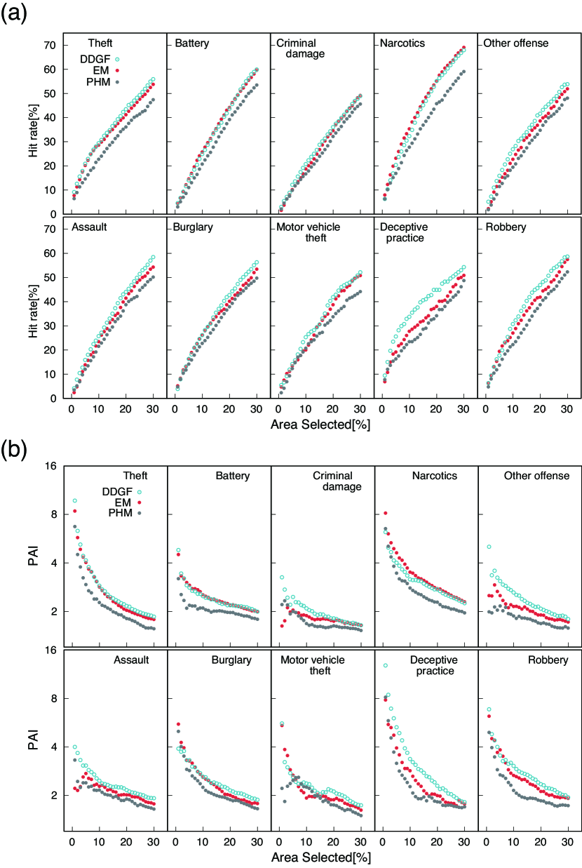
Figure 1: (a) Hit rate and (b) PAI of the one-day-ahead crime predictions as a function of area selected. The results of the PHM methods are derived without cutoff radius $r_{cut}$. The plots are obtained by averaging 50 calculations in shifting the prediction date once every other day, in order to increase the statistical reliability.

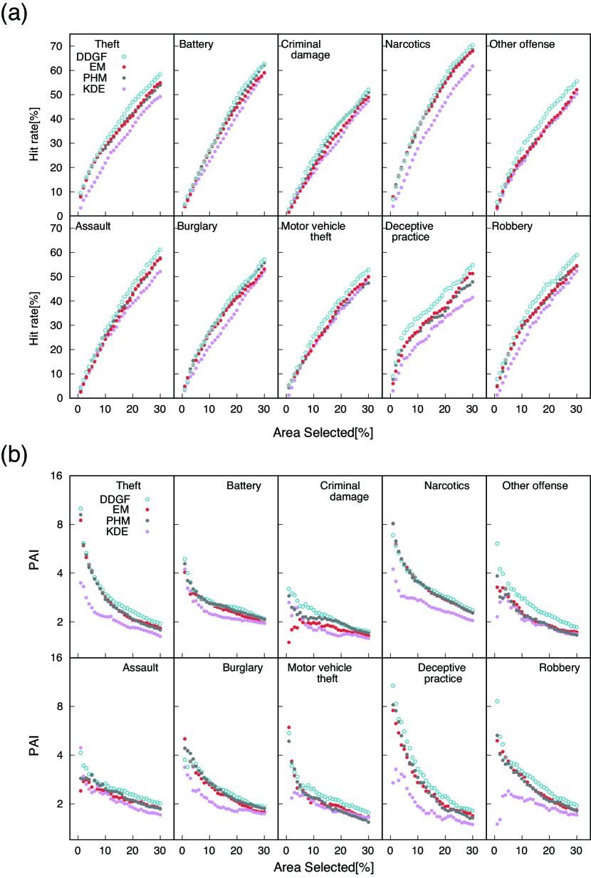
Figure 2: (a) Hit rate and (b) PAI of the one-day-ahead crime predictions as a function of area selected with the cutoff radius $r_{cut}=0.4$ km. The plots are obtained by averaging 50 calculations in shifting the prediction date once every other day, in order to increase the statistical reliability.

We use two types of metrics: hit rate and predictive accuracy index (PAI). The cells with the higher crime rate $\lambda(t,{\bf x})$ are selected up to a certain percentage $a/A$ of the total area, where $a$ is number of the selected cells. Then, the locations of the selected area and real crimes are checked if they are coincident. The hit rate is the correctly-predicted number of crimes divided by the total number of crimes as a function of $a/A$ which indicates percentage of the area selected [19, 36]. The PAI is defined as the hit rate divided by $a/A$ [38].

Table 1: Averaged hit rate and PAI of the one-day-ahead predictions in (upper table) Fig.1 and (bottom table) Fig.1. The bold number corresponds to the top accuracy between the three methods for each crime type.

	without $r_{cut}$
	Hit rate [%]			PAI
	DDGF	EM	PHM	DDGF	EM	PHM
Theft	36.1	34.6	29.3	3.00	2.85	2.33
Battery	34.6	35.0	30.1	2.47	2.49	2.06
Criminal damage	28.3	27.1	24.9	2.01	1.80	1.72
Narcotics	42.9	44.6	36.1	3.18	3.48	2.79
Other offense	33.5	30.5	27.3	2.47	2.07	1.80
Assault	34.7	32.1,	29.3	2.45	2.14	2.03
Burglary	34.3	32.7	30.2	2.52	2.52	2.28
Motor vehicle theft	31.9	30.3	26.7	2.32	2.22	1.95
Deceptive practice	38.5	32.5	29.1	3.57	2.77	2.49
Robbery	37.8	35.1	30.7	2.91	2.72	2.23

	$r_{cut}=0.4$ km
	Hit rate [%]				PAI
	DDGF	EM	PHM	KDE	DDGF	EM	PHM	KDE
Theft	37.9	35.3	35.1	29.3	3.11	2.90	2.91	2.1
Battery	37.3	35.2	36.7	32.6	2.67	2.49	2.61	2.31
Criminal damage	30.8	27.6	29.6	26.2	2.20	1.82	2.05	1.83
Narcotics	45.7	44.2	44.6	36.7	3.46	3.47	3.46	2.57
Other offense	34.9	30.5	30.3	29.6	2.67	2.21	2.18	2.06
Assault	36.4	33.4	34.1	30.9	2.53	2.23	2.33	2.18
Burglary	34.9	32.9	34.4	29.3	2.57	2.49	2.59	2.07
Motor-vehicle theft	32.5	29.8	29.0	28.6	2.36	2.20	2.15	1.9
Deceptive practice	37.5	33.2	32.2	26.9	3.43	2.85	2.97	1.96
Robbery	38.1	34.7	34.7	30.3	3.05	2.68	2.64	1.97

Table 2: Averaged hit rate and PAI of one-week-ahead prediction. The bold number corresponds to the top accuracy between the four methods for each crime type.

	$r_{cut}=0.4$ km
	Hit rate [%]				PAI
	DDGF	EM	PHM	KDE	DDGF	EM	PHM	KDE
Theft	37.9	34.8	34.8	28.9	3.06	2.77	2.81	2.04
Battery	37.3	34.0	36.4	32.8	2.65	2.4	2.59	2.3
Criminal damage	30.8	26.4	28.7	26.2	2.21	1.81	2.01	1.83
Narcotics	45.3	43.5	43.5	36.6	3.43	3.41	3.36	2.55
Other offense	35.5	30.7	30.8	30.2	2.7	2.19	2.19	2.13
Assault	35.9	31.0	33.5	31.0	2.53	2.1	2.28	2.2
Burglary	34.1	31.0	33.3	29.1	2.53	2.34	2.49	2.05
Motor-vehicle theft	32.6	29.5	29.5	28.2	2.39	2.19	2.19	1.88
Deceptive practice	38.8	32.2	31.4	26.6	3.41	2.68	2.72	1.94
Robbery	39.1	35.5	35.7	30.9	3.17	2.79	2.75	2.05

Here we compare the performaces of the DDGF, EM, and PHM methods in two manners with respect to the cutoff length $r_{cut}$, where $g(t,r>r_{cut})=0$. Figure 1 shows the hit rate and PAI without the cutoff parameter. Then, we introduce $r_{cut}=0.4$ km to these methods; the results are shown in Fig. 2. Note that the original PHM method uses $r_{cut}=0.4$ km [36], which was decided so as to be equivalent to the effective length of the near-repeat victimization [39, 40, 41]. Compared to this effective length of the near-repeat victimization, $\Delta x=0.25$ km is likely to be too large, in spite of the fact that this mesh is the finest in the available open data in Chicago. Owing to this large mesh, the DDGF and EM methods may give an erroneous broadening of $g(t,r)$ in $r$ direction. The introduction of $r_{cut}$, therefore, fixes this numerical artifacts to increase the scores of the DDGF and EM methods, not only of the PHM method. Indeed, Adepeju et al. [42] studied the same open data, and they used the cutoff $0.3$ km for their calculations of the EM method. Table 1 shows averages of these metrics over whole range of the area-selected rate $a/A=1,2,...,30\%$ in each of the crime types. The results shows that $r_{cut}$ parameter makes the accuracies of the three methods higher.

We also evaluate performance of the one-week-ahead prediction as shown in Table 2. The accuracies obtained by the DDGF method are superior to or comparable to the EM and PHM methods in both one-day and one-week ahead predictions.

6 Discussion

In order to clarify qualitative differences in these methods precisely, $g(t,r=0)$ is calculated from the larger burglary data using 450 days (from 16th March 2010 to 8th June 2011) extending the radius to 6 km. The total number of the burglary events is 9360. In the inset of Fig. 2, the DDGF and EM methods show the peaks at 1, 5, and 9 days and those at 1, 6, and 9 days, respectively. They give very similar profiles in the short-time region. These results indicate that the recidivism is likely to occur after the corresponding days counted from the first event.

A distinctive feature of the DDGF method can be observed in the long-time-scale behavior of $g(t,r=0)$. Figure 3 shows that $g(t,r=0)$ of the DDGF method decays very slowly in comparison to the EM and PHM methods, and this slow decay is well fitted by a logarithmic function (black line). The long-time tail feature is also found in earlier studies: some researchers collected cases of burglary that happened in the same location in order to analyze time intervals between the events, to shed light on the near-repeat victimization [45, 46, 47]. In particular, Ratcliffe et al. studied the data of burglaries in Nottinghamshire in UK for the period of 1995-1997 [47]. They found that the long-time-scale behavior of the observed distribution function of the time interval is well fitted with $-\log(t)$, as observed by the DDGF method here. Therefore, the observed logarithmic-like tail is an evidence that the DDGF method is able to describe the causal correlation of the crime events reasonably.

In addition to the hit rate and PAI, we use log-likelihoods to observe features of these models. The DDGF, PHM, and EM methods indicate the log-likelihoods averaged over all the crime types as 0.267, 0.273, and 0.292, respectively. The EM method shows the highest log-likelihood value. This is reasonable because the EM iteration step iterates in such a way to maximize the log-likelihood. Nevertheless, from a practical view point in the crime prediction, the hit rate and PAI are more important measures than log-likelihood. For example, police departments want to design an efficient patrol route due to a limited human resource to afford patrol activities. In this case, the log-likelihood is not suitable to be used, because this measure refers to similarity between "overall" distributions of $\lambda$ and crime events. On the other hand, the hit rate and PAI are indicators of the prediction performance defined even at a low percentage of the selected area. In fact, the hit rate or PAI are selected as standard measures in crime-prediction competitions and benchmark research[19, 42, 44], and some of the methods decide the model parameters so as to maximize these measures[31].

The kernel density estimation (KDE) method are also compared. We use the data amount for 400 days, which is the same condition as for the PHM, EM, and DDGF methods. The bandwidth is automatically decided by a standard rule-of-thumb scheme developed by Silverman [43]. The results are shown in Fig. 2, the lower table in Table 1, and Table 2. The prediction scores of the DDGF, EM, and PHM methods are larger than those of the KDE.

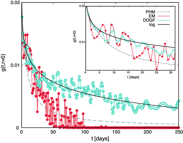
Figure 3: Profiles of $g(t,r=0)$ functions. The long-time-scale feature of the DDGF method is fitted by a logarithmic function of $-a\log(bt)$, where $a$ and $b$ are fitting parameters; the logarithmic function (black line) is overlaid. The inset figure shows the short-time-scale behaviors.

This study focused on the dynamic property described by a triggering kernel $g$ in Eq. (1) for the cascading effect. The background rate $\lambda_{0}$, which is the second term of the right-hand side in Eq. (1), is also an important term which describes a quasi-stationary influence of geometrical factors to the crime events. It represents influences from demographic factors (e.g., population and income distributions) and crime generators/attractors (e.g., bars and clubs)[48] in a city. A joint use of the triggering kernel and the background rate is essentially useful to predict crimes; this analysis will appear in our future work.

Here we put supplementary comments on the numerical aspects. The DDGF shows the best performance both for a day and week ahead conditions. If considering several months ahead condition, one obtains essentially zero $\lambda$ in the cases of PHM and EM methods, because the PHM has the 60-days cut off and the EM has a negligibly small $g$, as shown in Fig. 3. Only DDGF may show a non-zero $\lambda$ distribution due to the logarithmic long tail, though the $g$ is close to constant, which may leads to a poor prediction performance. With respect to the convergence sensitivity of the non-parametric model, both of the DDGF and EM methods are prone to produce unstable $\lambda$ in the case of small data, due to the high degrees of freedom in the function space for $g$. On the other hand, the parametric model is robust in terms of amount of data because of the fixed function form, though it has a poor flexibility of the representation ability of $g$.

7 Conclusion

We developed an algorithm that forecasts future crimes by learning the Green’s function from past data, combining the basis of the SEPP model. A systematic comparison with the standard methods, the EM and PHM is performed in terms of predicting one-day and one-week-ahead predictions for the 10 types of the crime in Chicago. The results show that DDGF exhibits a good prediction accuracy superior to or comparable to the standard methods. Furthermore, the DDGF method provided us with a characteristic long-time, logarithmic correlation of the crimes, which is consistent with the earlier study on burglaries. This long-tail feature cannot be reproduced by the other methods. Namely, the DDGF method enables us to mine the buried causal effects of crime events.

The DDGF method can be extended to multivariate in a matrix formalism. This extension enables us to apply cascading network phenomena such as financial time series, citation networks of scientific papers, and chain-reactive increase of users of social medias (e.g., Twitter), climatology, anomaly detection, demand forecasting in e-commerce, and biological signal data. The examples will appear in our future works.

References

References

- [1] W. L. Perry, Predictive policing: The role of crime forecasting in law enforcement operations, Rand Corporation, 2013. doi:10.7249/RR233.
- [2] M. L. Bonta, James, K. Hanson, The prediction of criminal and violent recidivism among mentally disordered offenders: a meta-analysis, Psychological bulletin 2 (1998) 123–142.
- [3] A. R. Baskin-Sommers, D. R. Baskin, I. B. Sommers, J. P. Newman, The intersectionality of sex, race, and psychopathology in predicting violent crimes, Criminal Justice and Behavior 40 (2013) 1068–1091. doi:10.1177/0093854813485412.
- [4] D. A. Andrews, J. Bonta, The psychology of criminal conduct, Routledge, 2014.
- [5] J. F. Edens, Interpersonal characteristics of male criminal offenders: Personality, psychopathological, and behavioral correlates, Psychological Assessment 21.1 (2009) 89–98. doi:10.1037/a0014856.
- [6] Harris, T. Stephanie, M. Marco, Picchioni, A review of the role of empathy in violence risk in mental disorders, Aggression and Violent Behavior 18 (2013) 335–342.
- [7] Krakowski, Menachem, J. Volavkaa, D. Brizera, Psychopathology and violence: A review of literature, Comprehensive Psychiatry 27 (2) (1986) 131–148.
- [8] L. W. Sherman, M. E. Buerger, Hot spots of predatory crime : routine activitices and the criminology of place, Criminology 27 (1) (1989) 27–56. doi:10.1111/j.1745-9125.1989.tb00862.x.
- [9] L. Anselin, J. Cohen, D. Cook, W. Gorr, G. Tita, Spatial analyses of crime, Criminal justice 4 (2) (2000) 213–262.
- [10] G. E. Tita, S. M. Radil, Spatializing the social networks of gangs to explore patterns of violence, Journal of Quantitative Criminology 27 (4) (2011) 521–545. doi:10.1007/s10940-011-9136-8.
- [11] T. Ohyama and M. Amemiya, Applying crime prediction techniques to japan: A comparison between risk terrain modeling and other methods, European Journal on Criminal Policy and Research (2018) 1–19doi:10.1007/s10610-018-9378-1.
- [12] M. S. Gerber, Predicting crime using twitter and kernel density estimation, Decision Support Systems 61 (2014) 115–125. doi:10.1016/j.dss.2014.02.003.
- [13] M. B. Short, M. R. D’orsogna, V. B. Pasour, G. E. Tita, P. J. Brantingham, A. L. Bertozzi, L. B. Chayes, A statistical model of criminal behavior, Mathematical Models and Methods in Applied Sciences 18 (supp01) (2008) 1249–1267. doi:10.1142/S0218202508003029.
- [14] G. L. Shoesmith, Space–time autoregressive models and forecasting national, regional and state crime rates, International journal of forecasting 29 (1) (2013) 191–201. doi:10.1016/j.ijforecast.2012.08.002.
- [15] T. P. Davies, S. R. Bishop, Modelling patterns of burglary on street networks, Crime Science 2 (1) (2013) 10. doi:10.1186/2193-7680-2-10.
- [16] A. Rodrigues, P. J. Diggle, Bayesian estimation and prediction for inhomogeneous spatiotemporal log-gaussian cox processes using low-rank models, with application to criminal surveillance, Journal of the American Statistical Association 107 (497) (2012) 93–101. doi:10.1080/01621459.2011.644496.
- [17] G. Mohler, Modeling and estimation of multi-source clustering in crime and security data, The Annals of Applied Statistics 7 (3) (2013) 1525–1539. doi:10.1214/13-AOAS647.
- [18] S. Shirota, A. E. Gelfand, et al., Space and circular time log gaussian cox processes with application to crime event data, The Annals of Applied Statistics 11 (2) (2017) 481–503.
- [19] G. O. Mohler, M. B. Short, P. J. Brantingham, F. P. Schoenberg, G. E. Tita, Self-exciting point process modeling of crime, Journal of the American Statistical Association 106 (493) (2011) 100–108. doi:10.1198/jasa.2011.ap09546.
- [20] G. Mohler, Marked point process hotspot maps for homicide and gun crime prediction in chicago, International Journal of Forecasting 30 (3) (2014) 491–497. doi:10.1016/j.ijforecast.2014.01.004.
- [21] D. J. Daley, D. Vere-Jones, An introduction to the theory of point processes: volume II: general theory and structure, Springer Science & Business Media, 2007.
- [22] S. D. Johnson, W. Bernasco, K. J. Bowers, H. Elffers, J. Ratcliffe, G. Rengert, M. Townsley, Space–time patterns of risk: a cross national assessment of residential burglary victimization, Journal of Quantitative Criminology 23 (3) (2007) 201–219. doi:10.1007/s10940-007-9025-3.
- [23] S. D. Johnson, Repeat burglary victimisation: a tale of two theories, Journal of Experimental Criminology 4(3) (2008) 215–240. doi:10.1007/s11292-008-9055-3.
- [24] M. B. Short, M. R. D’orsogna, P. J. Brantingham, G. E. Tita, Measuring and modeling repeat and near-repeat burglary effects, Journal of Quantitative Criminology 25 (3) (2009) 325–339. doi:10.1007/s10940-009-9068-8.
- [25] D. Marsan, O. Lengliné, Extending earthquakes’ reach through cascading, Science 319 (5866) (2008) 1076–1079. doi:10.1126/science.1148783.
- [26] D. Marsan, O. Lengliné, A new estimation of the decay of aftershock density with distance to the mainshock, Journal of Geophysical Research: Solid Earth 115 (B9). doi:10.1029/2009JB007119.
- [27] S. Aldor-Noiman, L. D. Brown, E. B. Fox, R. A. Stine, Spatio-temporal low count processes with application to violent crime events, Statistica Sinica 26 (2016) 1587–1610.
- [28] K. Zhou, H. Zha, L. Song, Learning triggering kernels for multi-dimensional hawkes processes, in: International Conference on Machine Learning, 2013, pp. 1301–1309.
- [29] S. Flaxman, A. Wilson, D. Neill, H. Nickisch, A. Smola, Fast kronecker inference in gaussian processes with non-gaussian likelihoods, in: International Conference on Machine Learning, 2015, pp. 607–616.
- [30] M. Eichler, R. Dahlhaus, J. Dueck, Graphical modeling for multivariate hawkes processes with nonparametric link functions, Journal of Time Series Analysis 38 (2) (2017) 225–242. doi:10.1111/jtsa.12213.
- [31] G. Mohler, M. D. Porter, Rotational grid, PAI-maximizing crime forecasts, no known publisher, 2017.
- [32] S. Flaxman, M. Chirico, P. Pereira, C. Loeffler, Scalable high-resolution forecasting of sparse spatiotemporal events with kernel methods: a winning solution to the nij" real-time crime forecasting challenge", arXiv preprint arXiv:1801.02858.
- [33] S. J. Farlow, Partial differential equations for scientists and engineers, John Wiley & Sons, Inc, 1982.
- [34] S. Kajita, Green’s function nonequilibrium molecular dynamics method for solid surfaces and interfaces, Physical Review E 94 (3) (2016) 033301. doi:10.1103/PhysRevE.94.033301.
- [35] W. Cai, M. de Koning, V. V. Bulatov, S. Yip, Minimizing boundary reflections in coupled-domain simulations, Physical Review Letters 85 (15) (2000) 3213–3216. doi:10.1103/PhysRevLett.85.3213.
- [36] K. J. Bowers, S. D. Johnson, K. Pease, Prospective hot-spotting: The future of crime mapping?, British Journal of Criminology 44 (5) (2004) 641–658. doi:10.1093/bjc/azh036.
- [37] City of chicago data portal, crimes, https://data.cityofchicago.org/Public-Safety/Crimes-2001-to-present/ijzp-q8t2.
- [38] S. Chainey, L. Tompson, S. Uhlig, The utility of hotspot mapping for predicting spatial patterns of crime, Security journal 21 (1-2) (2008) 4–28. doi:10.1057/palgrave.sj.8350066.
- [39] S. D. Johnson, K. J. Bowers, The burglary as clue to the future: The beginnings of prospective hot-spotting, European Journal of Criminology 1 (2) (2004) 237–255.
- [40] S. D. Johnson, K. J. Bowers, The stability of space-time clusters of burglary, British Journal of Criminology 44 (1) (2004) 55–65.
- [41] K. J. Bowers, S. D. Johnson, Domestic burglary repeats and space-time clusters: The dimensions of risk, European Journal of Criminology 2 (1) (2005) 67–92.
- [42] M. Adepeju, G. Rosser, T. Cheng, Novel evaluation metrics for sparse spatio-temporal point process hotspot predictions-a crime case study, International Journal of Geographical Information Science 30 (11) (2016) 2133–2154. doi:10.1080/13658816.2016.1159684.
- [43] B. W. Silverman, Density Estimation for Statistics and Data Analysis. London: Chapman & Hall/CRC. p. 45. (1986)ISBN:978-0-412-24620-3
- [44] “Real-Time Crime Forecasting Challenge”, which is a crime prediction contest held by NIJ adopted PAI as accuracy index. https://www.nij.gov/funding/Pages/fy16-crime-forecasting-challenge.aspx
- [45] D. Anderson, S. Chenery, K. Pease, Biting back: Tackling repeat burglary and car crime, Vol. 58, Home Office Police Research Group London, 1995.
- [46] R. Burquest, G. Farrell, K. Pease, Lessons from schools: some schools are repeatedly vandalised, and burgled. is there a pattern which police could interrupt?, Policing 8(2) (1992) 148–155.
- [47] J. H. Ratcliffe, M. J. McCullagh, Identifying repeat victimization with gis, The British Journal of Criminology 38 (4) (1998) 651–662. doi:10.1093/bjc/38.4.651.
- [48] W. Bernasco and R. Block, Robberies in Chicago: A block-level analysis of the influence of crime generators, crime attractors, and offender anchor points, Journal of Research in Crime and Delinquency, 48(1) (2011) 33-57. doi:10.1177/0022427810384135.
- [49] G. Fusai and A. Roncoroni, Implementing Models in Quantitative Finance: Methods and Cases, Springer Science and Business Media (2008) Capter 7. ISBN:978-3-540-22348-1.