Illuminating Light Bending

Abstract:

The interactions of gravitons with spin-1 matter are calculated in parallel with the well known photon case. It is shown that graviton scattering amplitudes can be factorized into a product of familiar electromagnetic forms, and cross sections for various reactions are straightforwardly evaluated using helicity methods. Universality relations are identified. Extrapolation to zero mass yields scattering amplitudes for photon-graviton and graviton-graviton scattering. The phenomenon of light bending near a massive object, which is generally treated using classical general relativity, is discussed from alternative points of view.

1 Introduction

The calculation of photon interactions with matter is part of any introductory (or advanced) course on quantum mechanics. Indeed the evaluation of the Compton scattering cross section is a standard exercise in relativistic quantum mechanics, since gauge invariance together with the masslessness of the photon allow the results to be presented in terms of relatively simple analytic forms [1].

One might expect a similar analysis to be applicable to the interactions of gravitons since, like photons, gravitons are massless and subject to a gauge invariance. Also, just as virtual photon exchange leads to a detailed understanding of electromagnetic interactions between charged systems, a careful treatment of virtual graviton exchange allows an understanding not just of Newtonian gravity, but also of spin-dependent phenomena—geodetic precession and Lense-Thirring frame dragging—associated with general relativity which have recently been verified by gravity probe B [2]. However, despite these parallels, examination of quantum mechanics texts reveals that (with one exception [3]) the case of graviton interactions is not discussed in any detail. There are at least three reasons for this situation:

• the graviton is a spin-two particle, as opposed to the spin-one photon, so that the interaction forms are more complex, involving symmetric and traceless second rank tensors rather than simple Lorentz four-vectors;

• there exist fewer experimental results with which to confront the theoretical calculations. Fundamental questions beyond the detection of quanta of gravitational fields have been exposed in [4];

• in order to guarantee gauge invariance one must include, in many processes, the contribution from a graviton pole term, involving a triple-graviton coupling. This vertex is a sixth rank tensor and contains a multitude of kinematic forms.

A century after the classical theory of general relativity and Einstein’s argument for a quantization of gravity [5], we are still seeking an experimental signature of quantum gravity effects. This paper presents and extends recent works, where elementary quantum gravity processes display new and very distinctive behaviors.

Recently, however, using powerful (string-based) techniques, which simplify conventional quantum field theory calculations, it has been demonstrated that the scattering of gravitons from an elementary target of arbitrary spin factorizes [6], a feature that had been noted ten years previously by Choi et al. based on gauge theory arguments [7]. This factorization property, which is sometime concisely described by the phrase “gravity is the square of a gauge theory”, permits a relatively elementary evaluation of various graviton amplitudes and opens the possibility of studying gravitational processes in physics coursework. In an earlier paper by one of us [8] it was shown explicitly how, for both spin-0 and spin-${1\over 2}$ targets, the use of factorization enables elementary calculation of both the graviton photoproduction,

$$\gamma+S\rightarrow g+S,$$

and gravitational Compton scattering,

$$g+S\rightarrow g+S,$$

reactions in terms of elementary photon reactions. This simplification means that graviton interactions can now be discussed in a basic quantum mechanics course and opens the possibility of treating interesting cosmological applications.

In the present paper we extend the work begun in [8] to the case of a spin-1 target and demonstrate and explain the origin of various universalities, i.e., results which are independent of target spin. In addition, by taking the limit of vanishing target mass we show how both graviton-photon and graviton-graviton scattering may be determined using elementary methods.

In section 2 then, we review the electromagnetic interactions of a spin one system. In section 3 we calculate the ordinary Compton scattering cross section for a spin-1 target and compare with the analogous spin-0 and spin-${1\over 2}$ forms. In section 4 we examine graviton photoproduction and gravitational Compton scattering for a spin-1 target and again compare with the analogous spin-0 and spin-${1\over 2}$ results. In section 5 we study the massless limit and show how both photon-graviton and graviton-graviton scattering can be evaluated, resolving a subtlety which arises in the derivation. Section 6 discusses some intriguing properties of the forward cross-section. In section 7 we review the classical physics calculation of the bending of light, including both lowest order and next to leading order corrections. After a derivation of the gravitational interaction of massless and massive systems in section 8, in section 9 we present at an alternative derivation in terms of geometrical optics, which uses the wave interpretation of light propagation. Then in section 10, we examine an additional way to derive the light bending, in terms of a quantum mechanical small angle scattering (eikonal) picture following the approach in [9]. A brief concluding section summarizes our results. The equivalence between results derived via these on the surface disparate techniques serves as an interesting example which can introduce students to new ways to analyze a familiar problem. Two appendices contain formalism and calculational details.

2 Spin One Interactions: a Lightning Review

We begin by reviewing the photon and graviton interactions of a spin-1 system. Recall that for a massive spin-0 system, we generate the photon interactions by writing down the free Lagrangian for a scalar field $\phi$

$${\cal L}_{0}^{S=0}=\partial_{\mu}\phi^{\dagger}\partial^{\mu}\phi-m^{2}\phi^{\dagger}\phi\,,$$ (1)

and making the minimal substitution [10]

$$i\partial_{\mu}\longrightarrow iD_{\mu}\equiv i\partial_{\mu}-eA_{\mu}\,.$$

This procedure leads to the familiar interaction Lagrangian

$${\cal L}_{int}^{S=0}=-iA_{\mu}\phi^{\dagger}\overleftrightarrow{\partial}^{\mu}\phi+e^{2}A^{\mu}A^{\nu}\eta_{\mu\nu}\phi^{\dagger}\phi\,,$$ (2)

where $e$ is the particle charge and $A_{\mu}$ is the photon field, and implies the one- and two-photon vertices

$$\langle p_{f}|V^{(1)\mu}_{em}|p_{i}\rangle = ie(p_{f}+p_{i})^{\mu},$$

$$\langle p_{f}|V^{(2)\mu\nu}_{em}|p_{i}\rangle = 2ie^{2}\eta^{\mu\nu}.$$ (3)

The corresponding charged massive spin-1 Lagrangian has the Proca form [11]

$${\cal L}_{0}^{S=1}=-{1\over 2}\,B^{\dagger}_{\mu\nu}B^{\mu\nu}+m^{2}\,B^{\dagger}_{\mu}B^{\mu}\,,$$ (4)

where $B^{\mu}$ is a spin one field subject to the constraint $\partial_{\mu}B^{\mu}=0$ and $B^{\mu\nu}$ is the antisymmetric tensor

$$B^{\mu\nu}=\partial^{\mu}B^{\nu}-\partial^{\nu}B^{\mu}\,.$$ (5)

The minimal substitution then leads to the interaction Lagrangian

$${\cal L}_{int}^{S=1}=i\,e\,A^{\mu}B^{\nu\dagger}\left(\eta_{\nu\alpha}\overleftrightarrow{\partial}_{\mu}-\eta_{\alpha\mu}\overleftrightarrow{\partial}_{\nu}\right)B^{\alpha}-e^{2}A^{\mu}A^{\nu}(\eta_{\mu\nu}\eta_{\alpha\beta}-\eta_{\mu\alpha}\eta_{\nu\beta})B^{\alpha\dagger}B^{\beta}\,,$$ (6)

and the one, two photon vertices

$$\big{\langle}p_{f},\epsilon_{B}\,\big{|}V_{em}^{(1)\mu}\big{|}\,p_{i},\epsilon_{A}\big{\rangle}_{S=1} = -i\,e\,\epsilon_{B\beta}^{*}\left((p_{f}+p_{i})^{\mu}\eta^{\alpha\beta}-\eta^{\beta\mu}p_{f}^{\alpha}-\eta^{\alpha\mu}p_{i}^{\beta}\right)\epsilon_{A\alpha}\,,$$

$$\big{\langle}p_{f},\epsilon_{B}\,\big{|}V_{em}^{(2)\mu\nu}\big{|}\,p_{i},\epsilon_{A}\big{\rangle}_{S=1} = i\,e^{2}\,\epsilon_{B\beta}^{*}\left(2\eta^{\alpha\beta}\eta^{\mu\nu}-\eta^{\alpha\mu}\eta^{\beta\nu}-\eta^{\alpha\nu}\eta^{\beta\mu}\right)\epsilon_{A\alpha}\,.$$ (7)

However, Eq. (7) is not the correct result for a fundamental spin-1 particle such as the charged $W$-boson. Because the $W$ arises in a gauge theory, the field tensor is not given by Eq. (5) but rather is generated from the charged—$\sqrt{1\over 2}(x\pm iy)$—component of

$$\bm{B}_{\mu\nu}=D_{\mu}\bm{B}_{\nu}-D_{\nu}\bm{B}_{\mu}-g_{ga}\bm{B}_{\mu}\times\bm{B}_{\nu}\,,$$ (8)

where $g_{ga}$ is the gauge coupling. This modification implies the existence of an additional $W^{\pm}\gamma$ interaction, leading to an “extra” contribution to the single photon vertex

$$\big{\langle}p_{f},\epsilon_{B}\,\big{|}\delta V_{em}^{(1)\mu}\big{|}\,p_{i},\epsilon_{A}\rangle_{S=1}=i\,e\,\epsilon_{B\beta}^{*}\left(\eta^{\alpha\mu}(p_{i}-p_{f})^{\beta}-\eta^{\beta\mu}(p_{i}-p_{f})^{\alpha})\right)\epsilon_{A\alpha}\,.$$ (9)

The significance of this term can be seen by using the mass-shell Proca constraints $p_{i}\cdot\epsilon_{A}=p_{f}\cdot\epsilon_{B}=0$ to write the total on-shell single photon vertex as

$$\big{\langle}p_{f},\epsilon_{B}\,\big{|}(V_{em}+\delta V_{em})^{\mu}\big{|}\,p_{i},\epsilon_{A}\big{\rangle}_{S=1} = -i\,e\,\epsilon_{B\beta}^{*}\left((p_{f}+p_{i})^{\mu}\eta^{\alpha\beta}-2\eta^{\beta\mu}(p_{i}-p_{f})^{\alpha}\right.$$ (10)

$$- \left.2\eta^{\alpha\mu}(p_{i}-p_{f})^{\beta}\right)\epsilon_{A\alpha}\,,$$

wherein, comparing with Eq. 9, we observe that the coefficient of the term $-\eta^{\alpha\mu}(p_{i}-p_{f})^{\beta}+\eta^{\beta\mu}(p_{i}-p_{f})^{\alpha}$ has been modified from unity to two. Since the rest frame spin operator can be identified via

$$B^{\dagger}_{i}B_{j}-B^{\dagger}_{j}B_{i}=-i\,\epsilon_{ijk}\big{\langle}f\,\big{|}S_{k}\big{|}\,i\big{\rangle}\,,$$ (12)

the corresponding piece of the nonrelativistic interaction Lagrangian becomes

$${\cal L}_{\rm int}=-g\,{e\over 2m}\big{\langle}f\,\big{|}\bm{S}\big{|}\,i\big{\rangle}\cdot\bm{\nabla}\times\bm{A}\,,$$ (13)

where $g$ is the gyromagnetic ratio and we have included a factor $2m$ which accounts for the normalization condition of the spin one field. Thus the “extra” interaction required by a gauge theory changes the $g$-factor from its Belinfante value of unity [12] to its universal value of two, as originally proposed by Weinberg [13] and more recently buttressed by a number of additional arguments [14]. Henceforth in this manuscript then we shall assume the $g$-factor of the spin-1 system to have its “natural” value $g=2$, since it is in this case that the high-energy properties of the scattering are well controlled and the factorization properties of gravitational amplitudes are valid [15].

3 Compton Scattering

The vertices given in the previous section can now be used to evaluate the ordinary Compton scattering amplitude,

$$\gamma+S\rightarrow\gamma+S,$$

for a spin-1 system having charge $e$ and mass $m$ by summing the contributions of the three diagrams shown in Figure 1, yielding

$${\rm Amp}^{\rm Comp}_{S=1} = 2e^{2}\Bigg{\{}\epsilon_{A}\cdot\epsilon_{B}^{*}\left[{\epsilon_{i}\cdot p_{i}\epsilon_{f}^{*}\cdot p_{f}\over p_{i}\cdot k_{i}}-{\epsilon_{i}\cdot p_{f}\epsilon_{f}^{*}\cdot p_{i}\over p_{i}\cdot k_{f}}-\epsilon_{i}\cdot\epsilon_{f}^{*}\right]$$ (14)

$$- \left[\epsilon_{A}\cdot[\epsilon_{f}^{*},k_{f}]\cdot\epsilon_{B}^{*}\left({\epsilon_{i}\cdot p_{i}\over p_{i}\cdot k_{i}}-{\epsilon_{i}\cdot p_{f}\over p_{i}\cdot k_{f}}\right)-\epsilon_{A}\cdot[\epsilon_{i},k_{i}]\cdot\epsilon_{B}^{*}\left({\epsilon_{f}\cdot p_{f}\over p_{i}\cdot k_{i}}-{\epsilon_{f}^{*}\cdot p_{i}\over p_{i}\cdot k_{f}}\right)\right]$$

$$- \left[{1\over p_{i}\cdot k_{i}}\epsilon_{A}\cdot[\epsilon_{i},k_{i}]\cdot[\epsilon_{f}^{*},k_{f}]\cdot\epsilon_{B}^{*}-{1\over p_{i}\cdot k_{f}}\epsilon_{A}\cdot[\epsilon_{f}^{*},k_{f}]\cdot[\epsilon_{i},k_{i}]\epsilon_{B}^{*}\right]\Bigg{\}},$$

with the momentum conservation condition $p_{i}+k_{i}=p_{f}+k_{f}$. We can verify the gauge invariance of the above form by noting that this amplitude can be written in the equivalent form

$${\rm Amp}_{S=1}^{\rm Comp} = {2e^{2}\over p_{i}\cdot k_{i}p_{i}\cdot k_{f}}\Bigg{\{}\epsilon_{B}^{*}\cdot\epsilon_{A}(p_{i}\cdot F_{i}\cdot F_{f}\cdot p_{i})$$ (15)

$$+ \Big{[}(\epsilon_{B}^{*}\cdot F_{f}\cdot\epsilon_{A})(p_{i}\cdot F_{i}\cdot p_{f})+(\epsilon_{B}^{*}\cdot F_{i}\cdot\epsilon_{A})(p_{i}\cdot F_{f}\cdot p_{f})\Big{]}$$

$$- \Big{[}p_{i}\cdot k_{f}(\epsilon_{B}^{*}\cdot F_{f}\cdot F_{i}\cdot\epsilon_{A})-p_{i}\cdot k_{i}(\epsilon_{B}^{*}\cdot F_{i}\cdot F_{f}\cdot\epsilon_{A})\Big{]}\Bigg{\}}\,,$$

where the electromagnetic field tensors are $F_{i}^{\mu\nu}=\epsilon_{i}^{\mu}k_{i}^{\nu}-\epsilon_{i}^{\nu}k_{i}^{\mu}$ and $F_{f}^{\mu\nu}=\epsilon_{f}^{*\mu}k_{f}^{\nu}-\epsilon_{f}^{*\nu}k_{f}^{\mu}$. Since $F_{i,f}$ are obviously invariant under the substitutions $\epsilon_{i,f}\rightarrow\epsilon_{i,f}+\lambda k_{i,f},\,\,i=1,2$, it is clear that Eq. (14) satisfies the gauge invariance strictures

$$\epsilon_{f}^{*\mu}k_{i}^{\nu}{\rm Amp}^{\rm Comp}_{\mu\nu,S=1}=k_{f}^{\mu}\epsilon_{i}^{\nu}{\rm Amp}^{\rm Comp}_{\mu\nu,S=1}=0\,.$$ (16)

Figure 1: Diagrams relevant to Compton scattering.

In order to make the transition to gravity, it is useful to utilize the helicity formalism [16], wherein one evaluates the matrix elements of the Compton amplitude between initial and final spin-1 and photon states having definite helicity, where helicity is defined as the projection of the particle spin along the momentum direction. We work initially in the center of mass frame and, for a photon incident with four-momentum $k_{i}^{\mu}=p_{\rm CM}(1,\hat{z})$, we choose the polarization vectors

$$\epsilon_{i}^{\lambda_{i}}=-{\lambda_{i}\over\sqrt{2}}\big{(}\hat{x}+i\lambda_{i}\hat{y}\big{)},\qquad\lambda_{i}=\pm\,,$$ (17)

while for an outgoing photon with $k_{f}^{\mu}=p_{\rm CM}(1,\cos\theta_{\rm CM}\hat{z}+\sin\theta_{\rm CM}\hat{x})$ we use polarizations

$$\epsilon_{f}^{\lambda_{f}}=-{\lambda_{f}\over\sqrt{2}}\Big{(}\cos\theta_{\rm CM}\hat{x}+i\lambda_{f}\hat{y}-\sin\theta_{\rm CM}\hat{z}\Big{)},\quad\lambda_{f}=\pm\,.$$ (18)

We can define corresponding helicity states for the spin-1 system. In this case the initial and final four-momenta are $p_{i}^{\mu}=(E_{\rm CM},-p_{\rm CM}\hat{z})$ and $p_{f}^{\mu}=\Big{(}E_{\rm CM},-p_{\rm CM}(\cos\theta_{\rm CM}\hat{z}+\sin\theta_{\rm CM}\hat{x})\Big{)}$ and there exist two transverse polarization four-vectors

$$\epsilon_{A}^{\pm\mu} = \Bigg{(}0,{\pm\hat{x}-i\hat{y}\over\sqrt{2}}\Bigg{)}\,,$$

$$\epsilon_{B}^{\pm\mu} = \Bigg{(}0,{\pm\cos\theta_{\rm CM}\hat{x}+i\hat{y}\mp\sin\theta_{\rm CM}\hat{z}\over\sqrt{2}}\Bigg{)}\,,$$ (19)

in addition to the longitudinal mode with polarization four-vectors

$$\epsilon_{A}^{0\mu} = {1\over m}\big{(}p_{\rm CM},-E_{\rm CM}\hat{z}\big{)}\,,$$

$$\epsilon_{B}^{0\mu} = {1\over m}\Big{(}p_{\rm CM},-E_{\rm CM}(\cos\theta_{\rm CM}\hat{z}+\sin\theta_{\rm CM}\hat{x})\Big{)}\,,$$ (20)

In terms of the usual invariant kinematic (Mandelstam) variables

$$s=\big{(}p_{i}+k_{i}\big{)}^{2},\quad t=\big{(}k_{i}-k_{f}\big{)}^{2},\quad u=\big{(}p_{i}-k_{f}\big{)}^{2}\,,$$ (21)

we identify

$$p_{\rm CM} = {s-m^{2}\over 2\sqrt{s}}\,,$$

$$E_{\rm CM} = {s+m^{2}\over 2\sqrt{s}}\,,$$

$$\cos{1\over 2}\theta_{\rm CM} = {\Big{(}(s-m^{2})^{2}+st\Big{)}^{1\over 2}\over s-m^{2}}={\Big{(}m^{4}-su\Big{)}^{1\over 2}\over s-m^{2}}\,,$$

$$\sin{1\over 2}\theta_{\rm CM} = {\big{(}-st\big{)}^{1\over 2}\over s-m^{2}}\,.$$ (22)

The invariant cross-section for unpolarized Compton scattering is then given by

$${d\sigma_{S=1}^{\rm Comp}\over dt}={1\over 16\pi(s-m^{2})^{2}}\ {1\over 3}\sum_{a,b=-,0,+}{1\over 2}\sum_{c,d=-,+}\Big{|}B^{1}(ab;cd)\Big{|}^{2}\,,\displaystyle$$ (23)

where

$$B^{1}(ab;cd)=\big{\langle}p_{f},b;k_{f},d\,\big{|}{\rm Amp}_{S=1}^{\rm Comp}\big{|}\,p_{i},a;k_{i},c\,\big{\rangle}\,,$$ (24)

is the Compton amplitude for scattering of a photon with four-momentum $k_{i}$, helicity a from a spin-1 target having four-momentum $p_{i}$, helicity $c$ to a photon with four-momentum $k_{f}$, helicity $d$ and target with four-momentum $p_{f}$, helicity $b$. The helicity amplitudes can now be calculated straightforwardly. There exist $3^{2}\times 2^{2}=36$ such amplitudes but, since helicity reverses under spatial inversion, parity invariance of the electromagnetic interaction requires that

$$\big{|}B^{1}(ab;cd)\big{|}=\big{|}B^{1}(-a-b;-c-d)\big{|}\,.$$

Also, since helicity is unchanged under time reversal, but initial and final states are interchanged, T-invariance of the electromagnetic interaction requires that

$$\big{|}B^{1}(ab;cd)\big{|}=\big{|}B^{1}(ba;dc)\big{|}\,.$$

Consequently there exist only twelve independent helicity amplitudes. Using Eq. (14) we calculate the various helicity amplitudes in the center of mass frame and then write these results in terms of invariants using Eq. (22), yielding

$$\big{|}B^{1}(++;++)\big{|} = \big{|}B^{1}(--;--)\big{|}=2e^{2}{\big{(}(s-m^{2})^{2}+m^{2}t\big{)}^{2}\over(s-m^{2})^{3}(u-m^{2})}\,,$$

$$\big{|}B^{1}(++;--)\big{|} = \big{|}B^{1}(--;++)\big{|}=2e^{2}{(m^{4}-su)^{2}\over(s-m^{2})^{3}(u-m^{2})}\,,$$

$$\big{|}B^{1}(+-;+-)\big{|} = \big{|}B^{1}(-+;-+)\big{|}=2e^{2}{m^{4}t^{2}\over(s-m^{2})^{3}(u-m^{2})}\,,$$

$$\big{|}B^{1}(+-;-+)\big{|} = \big{|}B^{1}(-+;+-)\big{|}=2e^{2}{s^{2}t^{2}\over(s-m^{2})^{3}(u-m^{2})}\,,$$

$$\big{|}B^{1}(++;+-)\big{|} = \big{|}B^{1}(--;-+)\big{|}=\big{|}B^{1}(++;-+)\big{|}=\big{|}B^{1}(--;+-)\big{|}\,,$$

$$= 2e^{2}{m^{2}t(m^{4}-su)\over(s-m^{2})^{3}(u-m^{2})}\,,$$

$$\big{|}B^{1}(+-;++)\big{|} = \big{|}B^{1}(-+;--)\big{|}=\big{|}B^{1}(-+;++)\big{|}=\big{|}B^{1}(+-;--)\big{|}\,,$$ (25)

$$= 2e^{2}{m^{2}t(m^{4}-su)\over(s-m^{2})^{3}(u-m^{2})}\,.$$

and

$$\big{|}B^{1}(0+;++)\big{|} = \big{|}B^{1}(0-;--)\big{|}=\big{|}B^{1}(+0;++)\big{|}=\big{|}B^{1}(-0;--)\big{|}\,,$$

$$= 2e^{2}{\sqrt{2}m\big{(}tm^{2}+(s-m^{2})^{2}\big{)}\sqrt{-t(m^{4}-su)}\over(s-m^{2})^{3}(u-m^{2})}\,,$$

$$\big{|}B^{1}(0+;+-)\big{|} = \big{|}B^{1}(0-;-+)\big{|}=\big{|}B^{1}(+0;-+)\big{|}=\big{|}B^{1}(-0;+-)\big{|}\,,$$

$$= 2e^{2}{\sqrt{2}mst\sqrt{-t(m^{4}-su)}\over(s-m^{2})^{3}(u-m^{2})}\,,$$

$$\big{|}B^{1}(0+;-+)\big{|} = \big{|}B^{1}(0-;+-)\big{|}=\big{|}B^{1}(+0;+-)\big{|}=\big{|}B^{1}(-0;-+)\big{|}\,,$$

$$= 2e^{2}{\sqrt{2}m^{3}t\sqrt{-t(m^{4}-su)}\over(s-m^{2})^{3}(u-m^{2})}\,,$$

$$\big{|}B^{1}(0+;--)\big{|} = \big{|}B^{1}(0-;++)\big{|}=\big{|}B^{1}(+0;--)\big{|}=\big{|}B^{1}(-0;++)\big{|}\,,$$

$$= 2e^{2}{\sqrt{2}m\big{(}-t(m^{4}-su)\big{)}^{3\over 2}\over(s-m^{2})^{3}t(u-m^{2})}\,,$$

$$\big{|}B^{1}(00;++)\big{|} = \big{|}B^{1}(00;--)\big{|}=2e^{2}{\big{(}2tm^{2}+(s-m^{2})^{2}\big{)}(m^{4}-su)\over(s-m^{2})^{3}(u-m^{2})}\,,$$

$$\big{|}B^{1}(00;+-)\big{|} = \big{|}B^{1}(00;-+)\big{|}=2e^{2}{\big{(}m^{2}t((s-m^{2})^{2}+2st\big{)}\over(s-m^{2})^{3}(u-m^{2})}\,.$$ (26)

Substitution into Eq. (23) then yields the invariant cross-section for unpolarized Compton scattering from a charged spin-1 target

$${d\sigma^{\rm Comp}_{S=1}\over dt}={e^{4}\over 12\pi(s-m^{2})^{4}(u-m^{2})^{2}}\Big{[}(m^{4}-su+t^{2})\big{(}3(m^{4}-su)+t^{2}\big{)}+t^{2}(t-m^{2})(t-3m^{2})\Big{]}\,,$$ (27)

which can be compared with the corresponding results for unpolarized Compton scattering from charged spin-0 and spin-$\frac{1}{2}$ targets found in ref. [8]—

$${d\sigma_{S=0}^{\rm Comp}\over dt} = {e^{4}\over 4\pi(s-m^{2})^{4}(u-m^{2})^{2}}\left[(m^{4}-su)^{2}+m^{4}t^{2}\right]\,,$$

$${d\sigma_{S={1\over 2}}^{\rm Comp}\over dt} = {e^{4}\over 8\pi{(s-m^{2})^{4}(u-m^{2})^{2}}}\Big{[}(m^{4}-su)\big{(}2(m^{4}-su)+t^{2}\big{)}+m^{2}t^{2}(2m^{2}-t)\Big{]}\,.$$

(28)

Often such results are written in the laboratory frame, wherein the target is at rest, by use of the relations

$$s-m^{2} = 2m\omega_{i},\quad u-m^{2}=-2m\omega_{f}\,,$$

$$m^{4}-su = 4m^{2}\omega_{i}\omega_{f}\cos^{2}{\theta_{L}\over 2},\quad m^{2}t=-4m^{2}\omega_{i}\omega_{f}\sin^{2}{\theta_{L}\over 2}\,,$$ (29)

and

$${dt\over d\Omega}={d\over 2\pi d\cos\theta_{L}}\left(-{2\omega_{i}^{2}(1-\cos\theta_{L})\over 1+{\omega_{i}\over m}(1-\cos\theta_{L})}\right)={\omega_{f}^{2}\over\pi}\,.$$ (30)

Introducing the fine structure constant $\alpha=e^{2}/4\pi$, we find then

$${d\sigma_{{\rm lab},S=1}^{\rm Comp}\over d\Omega} = {\alpha^{2}\over m^{2}}{\omega_{f}^{4}\over\omega_{i}^{4}}\left[\bigg{(}\cos^{4}{\theta_{L}\over 2}+\sin^{4}{\theta_{L}\over 2}\bigg{)}\bigg{(}1+2{\omega_{i}\over m}\sin^{2}{\theta_{L}\over 2}\bigg{)}^{2}\right.$$

$$+ \left.{16\omega_{i}^{2}\over 3m^{2}}\sin^{4}{\theta_{L}\over 2}\bigg{(}1+2{\omega_{i}\over m}\sin^{2}{\theta_{L}\over 2}\bigg{)}+{32\omega_{i}^{4}\over 3m^{4}}\sin^{8}{\theta_{L}\over 2}\right]\,,$$

$${d\sigma^{\rm Comp}_{{\rm lab},S={1\over 2}}\over d\Omega} = {\alpha^{2}\over m^{2}}{\omega_{f}^{3}\over\omega_{i}^{3}}\left[\bigg{(}\cos^{4}{\theta_{L}\over 2}+\sin^{4}{\theta_{L}\over 2}\bigg{)}\bigg{(}1+2{\omega_{i}\over m}\sin^{2}{\theta_{L}\over 2}\bigg{)}+2{\omega_{i}^{2}\over m^{2}}\sin^{4}{\theta_{L}\over 2}\right]\,,$$

$${d\sigma^{\rm Comp}_{{\rm lab},S=0}\over d\Omega} = {\alpha^{2}\over m^{2}}{\omega_{f}^{2}\over\omega_{i}^{2}}\left[\cos^{4}{\theta_{L}\over 2}+\sin^{4}{\theta_{L}\over 2}\right]\,.$$ (31)

We observe that the nonrelativistic laboratory cross-section has an identical form for any spin

$$\left.{d\sigma_{{\rm lab},S}^{\rm Comp}\over d\Omega}\right|^{NR}={\alpha^{2}\over m^{2}}\left[\bigg{(}\cos^{4}{\theta_{L}\over 2}+\sin^{4}{\theta_{L}\over 2}\Big{)}\Big{(}1+{\cal O}\Big{(}{\omega_{i}\over m}\Big{)}\bigg{)}\right]\,,$$ (32)

which follows from the universal form of the Compton amplitude for scattering from a spin-$S$ target in the low-energy ($\omega\ll m$) limit, which in turn arises from the universal form of the Compton amplitude for scattering from a spin-$S$ target in the low-energy limit—

$$\big{\langle}S,M_{f};\epsilon_{f}\,\big{|}{\rm Amp}^{\rm Comp}_{S}\big{|}\,S,M_{i};\epsilon_{i}\big{\rangle}_{\omega\ll m}=2e^{2}\,\epsilon_{f}^{*}\cdot\epsilon_{i}\,\delta_{M_{i},M_{f}}+\ldots\,,$$ (33)

which obtains in an effective field theory approach to Compton scattering [17].

4 Gravitational Interactions

In the previous section we discussed the treatment the familiar electromagnetic interaction, using Compton scattering on a spin-1 target as an example. In this section we show how the gravitational interaction can be evaluated via methods parallel to those used in the electromagnetic case. An important difference is that while in the electromagnetic case we have the simple interaction Lagrangian

$${\cal L}_{int}=-eA_{\mu}J^{\mu}\,,$$ (35)

where $J^{\mu}$ is the electromagnetic current matrix element, for gravity we have

$${\cal L}_{int}={\kappa\over 2}h_{\mu\nu}T^{\mu\nu}\,.$$ (36)

Here the field tensor $h_{\mu\nu}$ is defined in terms of the metric via

$$g_{\mu\nu}=\eta_{\mu\nu}+\kappa h_{\mu\nu}\,,$$ (37)

where $\kappa$ is given in terms of the Cavendish constant $G$ by $\kappa^{2}=32\pi G$. The Einstein-Hilbert action is

$$\mathcal{S}_{\rm Einstein-Hilbert}=\int d^{4}x\,\sqrt{-g}\,{2\over\kappa^{2}}\,R\,,$$ (38)

where

$$\sqrt{-g}\equiv\sqrt{-{\rm det}\,g}=\exp{1\over 2}{\rm tr}{\rm log}\,g=1+{1\over 2}\eta^{\mu\nu}h_{\mu\nu}+\ldots\,,$$ (39)

is the square root of the determinant of the metric and $R=R^{\lambda}{}_{\mu\lambda\nu}g^{\mu\nu}$ is the Ricci scalar curvature obtained by contracting the Riemann tensor $R^{\mu}{}_{\nu\rho\sigma}$ with the metric tensor. The energy-momentum tensor is defined in terms of the matter Lagrangian via

$$T_{\mu\nu}={2\over\sqrt{-g}}{\delta{\sqrt{-g}\cal L}_{\rm mat}\over\delta g^{\mu\nu}}\,.$$ (40)

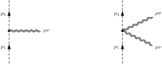
Figure 2: (a) The one-graviton and (b) two-graviton emission vertices from either a scalar, spinor or vector particle.

The spin-1 single graviton emission vertex shown in figure 2(a) can now be identified

$$\big{\langle}p_{f},\epsilon_{B}\,\big{|}V_{grav}^{(1)\mu\nu}\big{|}\,p_{i},\epsilon_{A}\big{\rangle}_{S=1} = -i\,{\kappa\over 2}\,\bigg{[}\epsilon_{B}^{*}\cdot\epsilon_{A}\big{(}p_{i}^{\mu}p_{f}^{\nu}+p_{i}^{\nu}p_{f}^{\mu}\big{)}-\epsilon_{B}^{*}\cdot p_{i}\,\big{(}p_{f}^{\mu}\epsilon_{A}^{\nu}+\epsilon_{A}^{\mu}p_{f}^{\nu}\big{)}$$ (41)

$$- \epsilon_{A}\cdot p_{f}\big{(}p_{i}^{\nu}\epsilon_{B}^{*\mu}+p_{i}^{\mu}\epsilon_{B}^{*\nu}\big{)}+\big{(}p_{f}\cdot p_{i}-m^{2}\big{)}\big{(}\epsilon_{A}^{\mu}\epsilon_{B}^{*\nu}+\epsilon_{A}^{\nu}\epsilon_{B}^{*\mu}\big{)}$$

$$- \eta^{\mu\nu}\Big{[}\big{(}p_{i}\cdot p_{f}-m^{2}\big{)}\epsilon_{B}^{*}\cdot\epsilon_{A}-\epsilon_{B}^{*}\cdot p_{i}\,\epsilon_{A}\cdot p_{f}\Big{]}\bigg{]}\,.$$

There also exist two-graviton (seagull) vertices shown in figure 2(b), which can be found by expanding the stress-energy tensor to second order in $h_{\mu\nu}$.

$$\big{\langle}p_{f},\epsilon_{B};k_{f}\,\big{|}V_{grav}^{(2)\,\mu\nu,\rho\sigma}\big{|}\,p_{i},\epsilon_{A};k_{i}\big{\rangle}_{S=1}\!\!\!\!=-i\,{\kappa^{2}\over 4}\epsilon_{A}^{\alpha}(\epsilon_{B}^{\beta})^{*}\,\Bigg{\{}$$ (42)

$$+ \Big{[}p_{i\beta}p_{f\alpha}-\left.\eta_{\alpha\beta}(p_{i}\cdot p_{f}-m^{2})\Big{]}\Big{(}\eta_{\mu\rho}\eta_{\nu\sigma}+\eta_{\mu\sigma}\eta_{\nu\rho}-\eta_{\mu\nu}\eta_{\rho\sigma}\Big{)}\right.$$

$$+ \left.\eta_{\mu\rho}\Big{[}\eta_{\alpha\beta}\Big{(}p_{i\nu}p_{f\sigma}+p_{i\sigma}p_{f\nu}\Big{)}-\eta_{\alpha\nu}p_{i\beta}p_{f\sigma}-\eta_{\beta\nu}p_{i\sigma}p_{f\alpha}\right.$$

$$- \left.\eta_{\beta\sigma}p_{i\nu}p_{f\alpha}-\eta_{\alpha\sigma}p_{i\beta}p_{f\nu}+(p_{i}\cdot p_{f}-m^{2}\Big{)}\Big{(}\eta_{\alpha\nu}\eta_{\beta\sigma}+\eta_{\alpha\sigma}\eta_{\beta\nu}\Big{)}\Big{]}\right.$$

$$+ \left.\eta_{\mu\sigma}\Big{[}\eta_{\alpha\beta}\Big{(}p_{i\nu}p_{f\rho}+p_{i\rho}p_{f\nu}\Big{)}-\eta_{\alpha\nu}p_{i\beta}p_{f\rho}-\eta_{\beta\nu}p_{i\rho}p_{f\alpha}\right.$$

$$- \left.\eta_{\beta\rho}p_{i\nu}p_{f\alpha}-\eta_{\alpha\rho}p_{i\beta}p_{f\nu}+(p_{i}\cdot p_{f}-m^{2}\Big{)}\eta_{\alpha\nu}\eta_{\beta\rho}+\eta_{\alpha\rho}\eta_{\beta\nu}\Big{)}\Big{]}\right.$$

$$+ \left.\eta_{\nu\rho}\Big{[}\eta_{\alpha\beta}\Big{(}p_{i\mu}p_{f\sigma}+p_{i\sigma}p_{f\mu}\Big{)}-\eta_{\alpha\mu}p_{i\beta}p_{f\sigma}-\eta_{\beta\mu}p_{i\sigma}p_{f\alpha}\right.$$

$$- \left.\eta_{\beta\sigma}p_{i\mu}p_{f\alpha}-\eta_{\alpha\sigma}p_{i\beta}p_{f\mu}+(p_{i}\cdot p_{f}-m^{2}\Big{)}\Big{(}\eta_{\alpha\mu}\eta_{\beta\sigma}+\eta_{\alpha\sigma}\eta_{\beta\mu}\Big{)}\Big{]}\right.$$

$$+ \left.\eta_{\nu\sigma}\Big{[}\eta_{\alpha\beta}\Big{(}p_{i\mu}p_{f\rho}+p_{i\rho}p_{f\mu}\Big{)}-\eta_{\alpha\mu}p_{i\beta}p_{f\rho}-\eta_{\beta\mu}p_{i\rho}p_{f\alpha}\right.$$

$$- \left.\eta_{\beta\rho}p_{i\mu}p_{f\alpha}-\eta_{\alpha\rho}p_{i\beta}p_{f\mu}+(p_{i}\cdot p_{f}-m^{2}\Big{)}\Big{(}\eta_{\alpha\mu}\eta_{\beta\rho}+\eta_{\alpha\rho}\eta_{\beta\mu}\Big{)}\Big{]}\right.$$

$$- \left.\eta_{\mu\nu}\Big{[}\eta_{\alpha\beta}\Big{(}p_{i\rho}p_{f\sigma}+p_{i\sigma}p_{f\rho}\Big{)}-\eta_{\alpha\rho}p_{i\beta}p_{f\sigma}-\eta_{\beta\rho}p_{i\sigma}p_{f\alpha}\right.$$

$$- \left.\eta_{\beta\sigma}p_{i\rho}p_{f\alpha}-\eta_{\alpha\sigma}p_{i\beta}p_{f\rho}+\Big{(}p_{i}\cdot p_{f}-m^{2}\Big{)}\Big{(}\eta_{\alpha\rho}\eta_{\beta\sigma}+\eta_{\beta\rho}\eta_{\alpha\sigma}\Big{)}\Big{]}\right.$$

$$- \left.\eta_{\rho\sigma}\Big{[}\eta_{\alpha\beta}\Big{(}p_{i\mu}p_{f\nu}+p_{i\nu}p_{f\mu}\Big{)}-\eta_{\alpha\mu}p_{i\beta}p_{f\nu}-\eta_{\beta\mu}p_{i\nu}p_{f\alpha}\right.$$

$$- \left.\eta_{\beta\nu}p_{i\mu}p_{f\alpha}-\eta_{\alpha\nu}p_{i\beta}p_{f\mu}+(p_{i}\cdot p_{f}-m^{2}\Big{)}\Big{(}\eta_{\alpha\mu}\eta_{\beta\nu}+\eta_{\beta\mu}\eta_{\alpha\nu}\Big{)}\Big{]}\right.$$

$$+ \left.\Big{(}\eta_{\alpha\rho}p_{i\mu}-\eta_{\alpha\mu}p_{i\rho}\Big{)}\Big{(}\eta_{\beta\sigma}p_{f\nu}-\eta_{\beta\mu}p_{f\sigma}\Big{)}\right.$$

$$+ \left.\Big{(}\eta_{\alpha\sigma}p_{i\nu}-\eta_{\alpha\nu}p_{i\sigma}\Big{)}\Big{(}\eta_{\beta\rho}p_{f\mu}-\eta_{\beta\mu}p_{f\rho}\Big{)}\right.$$

$$+ \left.\Big{(}\eta_{\alpha\sigma}p_{i\mu}-\eta_{\alpha\mu}p_{i\sigma}\Big{)}\Big{(}\eta_{\beta\rho}p_{f\nu}-\eta_{\beta\nu}p_{f\rho}\Big{)}\right.$$

$$+ \Big{(}\eta_{\alpha\rho}p_{i\nu}-\eta_{\alpha\nu}p_{i\rho}\Big{)}\Big{(}\eta_{\beta\sigma}p_{f\mu}-\eta_{\beta\mu}p_{f\sigma}\Big{)}\Bigg{\}}\,.$$

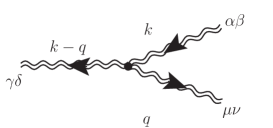
Figure 3: The three graviton vertex

Finally, we require the triple graviton vertex of figure 3

$$\tau^{\mu\nu}_{\alpha\beta,\gamma\delta}(k,q)\!\!\!\! = \!\!\!-{i\,\kappa\over 2}\left[\big{(}I_{\alpha\beta,\gamma\delta}-{1\over 2}\eta_{\alpha\beta}\eta_{\gamma\delta}\big{)}\left.\bigg{[}k^{\mu}k^{\nu}+(k-q)^{\mu}(k-q)^{\nu}+q^{\mu}q^{\nu}-{3\over 2}\eta^{\mu\nu}q^{2}\right]\right.$$ (43)

$$+ \left.2q_{\lambda}q_{\sigma}\left.\Big{[}I^{\lambda\sigma,}{}_{\alpha\beta}I^{\mu\nu,}{}_{\gamma\delta}+I^{\lambda\sigma,}{}_{\gamma\delta}I^{\mu\nu,}{}_{\alpha\beta}-I^{\lambda\mu,}{}_{\alpha\beta}I^{\sigma\nu,}{}_{\gamma\delta}-I^{\sigma\nu,}{}_{\alpha\beta}I^{\lambda\mu,}{}_{\gamma\delta}\right]\right.$$

$$+ \left.\Big{[}q_{\lambda}q^{\mu}\big{(}\eta_{\alpha\beta}I^{\lambda\nu,}{}_{\gamma\delta}+\eta_{\gamma\delta}I^{\lambda\nu,}{}_{\alpha\beta})+q_{\lambda}q^{\nu}(\eta_{\alpha\beta}I^{\lambda\mu,}{}_{\gamma\delta}+\eta_{\gamma\delta}I^{\lambda\mu,}{}_{\alpha\beta}\big{)}\right.$$

$$- \left.q^{2}\big{(}\eta_{\alpha\beta}I^{\mu\nu,}{}_{\gamma\delta}+\eta_{\gamma\delta}I^{\mu\nu,}{}_{\alpha\beta})-\eta^{\mu\nu}q^{\lambda}q^{\sigma}(\eta_{\alpha\beta}I_{\gamma\delta,\lambda\sigma}+\eta_{\gamma\delta}I_{\alpha\beta,\lambda\sigma}\big{)}\Big{]}\right.$$

$$+ \left.\Big{[}2q^{\lambda}\big{(}I^{\sigma\nu,}{}_{\gamma\delta}I_{\alpha\beta,\lambda\sigma}(k-q)^{\mu}\!+\!I^{\sigma\mu,}{}_{\gamma\delta}I_{\alpha\beta,\lambda\sigma}(k-q)^{\nu}\right.\!-\!\left.I^{\sigma\nu,}{}_{\alpha\beta}I_{\gamma\delta,\lambda\sigma}k^{\mu}\!-\!I^{\sigma\mu,}{}_{\alpha\beta}I_{\gamma\delta,\lambda\sigma}k^{\nu}\big{)}\right.$$

$$+ \left.q^{2}\big{(}I^{\sigma\mu,}{}_{\alpha\beta}I_{\gamma\delta,\sigma}{}^{\nu}+I_{\alpha\beta,\sigma}{}^{\nu}I^{\sigma\mu,}{}_{\gamma\delta}\big{)}+\eta^{\mu\nu}q^{\lambda}q_{\sigma}\big{(}I_{\alpha\beta,\lambda\rho}I^{\rho\sigma,}{}_{\gamma\delta}+I_{\gamma\delta,\lambda\rho}I^{\rho\sigma,}{}_{\alpha\beta}\big{)}\Big{]}\right.$$

$$+ \left.\Big{[}\big{(}k^{2}+(k-q)^{2}\big{)}\left(I^{\sigma\mu,}{}_{\alpha\beta}I_{\gamma\delta,\sigma}{}^{\nu}+I^{\sigma\nu,}{}_{\alpha\beta}I_{\gamma\delta,\sigma}{}^{\mu}-{1\over 2}\eta^{\mu\nu}\big{(}I_{\alpha\beta,\gamma\delta}-{1\over 2}\eta_{\alpha\beta}\eta_{\gamma\delta})\right.\big{)}\right.$$

$$- \left.\big{(}k^{2}\eta_{\alpha\beta}I^{\mu\nu,}{}_{\gamma\delta}+(k-q)^{2}\eta_{\gamma\delta}I^{\mu\nu,}{}_{\alpha\beta}\big{)}\Big{]}\right.\bigg{]}\,,$$

where

$$I_{\alpha\beta,\gamma\delta}={1\over 2}(\eta_{\alpha\gamma}\eta_{\beta\delta}+\eta_{\alpha\delta}\eta_{\beta\gamma})\,.$$ (44)

We work in harmonic (de Donder) gauge which satisfies, in lowest order,

$$\partial^{\mu}h_{\mu\nu}={1\over 2}\partial_{\nu}h\,,$$ (45)

with

$$h\equiv{\rm tr}\,h_{\mu\nu}\,,$$ (46)

in which the graviton propagator has the form

$$D_{\alpha\beta;\gamma\delta}(q)={i\over q^{2}+i\epsilon}{1\over 2}(\eta_{\alpha\gamma}\eta_{\beta\delta}+\eta_{\alpha\delta}\eta_{\beta\gamma}-\eta_{\alpha\beta}\eta_{\gamma\delta})\,.$$ (47)

Then just as the (massless) photon is described in terms of a spin-1 polarization vector $\epsilon_{\mu}$ which can have projection (helicity) either plus- or minus-1 along the momentum direction, the (massless) graviton is a spin-2 particle which can have the projection (helicity) either plus- or minus-2 along the momentum direction. Since $h_{\mu\nu}$ is a symmetric tensor, it can be described in terms of a direct product of unit spin polarization vectors—

$${\rm helicity} = +2:\quad h^{(2)}_{\mu\nu}=\epsilon^{+}_{\mu}\epsilon^{+}_{\nu}\,,$$

$${\rm helicity} = -2:\quad h^{(-2)}_{\mu\nu}=\epsilon^{-}_{\mu}\epsilon^{-}_{\nu}\,,$$ (48)

and, just as in electromagnetism, there is a gauge condition—in this case Eq. (45)—which must be satisfied. Note that the helicity states given in Eq. (48) are consistent with the gauge requirement since

$$\eta^{\mu\nu}\epsilon_{\mu}^{+}\epsilon_{\nu}^{+}=\eta^{\mu\nu}\epsilon_{\mu}^{-}\epsilon_{\nu}^{-}=0,\quad{\rm and}\quad k^{\mu}\epsilon_{\mu}^{\pm}=0\,.$$ (49)

With this background we can now examine specific graviton reactions.

4.1 Graviton Photo-production

We first use the above results to discuss the problem of graviton photo-production on a spin-1 target—$\gamma+S\rightarrow g+S$—for which the relevant four diagrams are shown in Figure 4. The electromagnetic and gravitational vertices needed for the Born terms and photon pole diagrams—Figures 4a, 4b, and 4d—have been given above. For the photon pole diagram we require the graviton-photon coupling, which can be found from the electromagnetic energy-momentum tensor [10]

$$T_{\mu\nu}=-F_{\mu\alpha}F^{\alpha}_{\nu}+{1\over 4}g_{\mu\nu}F_{\alpha\beta}F^{\alpha\beta}\,,$$ (50)

and yields the photon-graviton vertex

$$\big{\langle}k_{f},\epsilon_{f}\,\big{|}V_{grav}^{(\gamma)\mu\nu}\big{|}\,k_{i},\epsilon_{i}\big{\rangle} = i\,{\kappa\over 2}\left.\Big{[}\epsilon_{f}^{*}\cdot\epsilon_{i}\big{(}k_{i}^{\mu}k_{f}^{\nu}+k_{i}^{\nu}k_{f}^{\mu}\big{)}-\epsilon_{f}^{*}\cdot k_{i}\big{(}k_{f}^{\mu}\epsilon_{i}^{\nu}+\epsilon_{i}^{\mu}k_{f}^{\nu}\big{)}\right.$$ (51)

$$- \left.\epsilon_{i}\cdot k_{f}\big{(}k_{i}^{\nu}\epsilon_{f}^{*\mu}+k_{i}^{\mu}\epsilon_{f}^{*\nu}\big{)}+k_{f}\cdot k_{i}\big{(}\epsilon_{i}^{\mu}\epsilon_{f}^{*\nu}+\epsilon_{i}^{\nu}\epsilon_{f}^{*\mu}\big{)}\right.$$

$$- \left.\eta^{\mu\nu}\left[k_{f}\cdot k_{i}\epsilon_{f}^{*}\cdot\epsilon_{i}-\epsilon_{f}^{*}\cdot k_{i}\epsilon_{i}\cdot k_{f}\right]\right.\Big{]}\,.$$

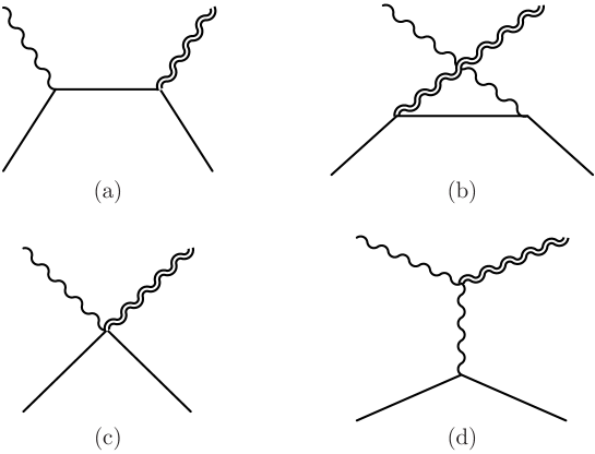
Figure 4: Diagrams relevant to graviton photo-production.

Finally, we need the seagull vertex which arises from the feature that the energy-momentum tensor depends on $p_{i},p_{f}$ and therefore yields a contact interaction when the minimal substitution is made, yielding the spin-1 seagull amplitude shown in Figure 4c.

$$\big{\langle}p_{f},\epsilon_{B};k_{f},\epsilon_{f}\epsilon_{f}\,\big{|}T\big{|}\,p_{i},\epsilon_{A};k_{i},\epsilon_{i}\big{\rangle}_{\rm seagull}=\,{i\over 2}\,\kappa\,e\left.\Big{[}\epsilon_{f}^{*}\cdot(p_{f}+p_{i})\,\epsilon_{f}^{*}\cdot\epsilon_{i}\,\epsilon_{B}^{*}\cdot\epsilon_{A}\,\right.$$ (52)

$$- \left.\epsilon_{B}^{*}\cdot\epsilon_{i}\,\epsilon_{f}^{*}\cdot p_{f}\,\epsilon_{f}^{*}\cdot\epsilon_{A}-\epsilon_{B}^{*}\cdot p_{i}\,\epsilon_{f}^{*}\cdot\epsilon_{i}\,\epsilon_{f}^{*}\cdot\epsilon_{A}-\epsilon_{A}\cdot\epsilon_{i}\,\epsilon_{f}^{*}\cdot p_{i}\,\epsilon_{f}^{*}\cdot\epsilon_{B}^{*}\right.$$

$$- \left.\epsilon_{A}\cdot p_{f}\,\epsilon_{f}^{*}\cdot\epsilon_{i}\,\epsilon_{f}^{*}\cdot\epsilon_{B}^{*}-\epsilon_{f}^{*}\cdot\epsilon_{A}\,\epsilon_{i}\cdot(p_{f}+p_{i})\,\epsilon_{f}^{*}\cdot\epsilon_{B}^{*}\right.\Big{]}\,.$$

The individual contributions from the four diagrams in Figure 4 are given in Appendix B and have a rather complex form. However, when added together we find a much simpler result. The full graviton photo-production amplitude is found to be proportional to the already calculated Compton amplitude for spin-1—Eq. (14)—times a universal kinematic factor. That is,

$$\big{\langle}p_{f};k_{f},\epsilon_{f}\epsilon_{f}\big{|}T\big{|}p_{i};k_{i},\epsilon_{i}\big{\rangle}=\sum_{i=a,b,c,d}{\rm Amp}\,({\rm Fig}.4(i))=H\times\left(\epsilon_{f\alpha}^{*}\epsilon_{i\beta}T_{\rm Compton}^{\alpha\beta}(S=1)\right)\,,$$ (53)

where

$$H={\kappa\over 2e}{p_{f}\cdot F_{f}\cdot p_{i}\over k_{i}\cdot k_{f}}={\kappa\over 2e}\,{\epsilon_{f}^{*}\cdot p_{f}\,k_{f}\cdot p_{i}-\epsilon_{f}^{*}\cdot p_{i}\,k_{f}\cdot p_{f}\over k_{i}\cdot k_{f}}\,,$$ (54)

and $\epsilon_{f\alpha}^{*}\epsilon_{i\beta}T_{\rm Compton}^{\alpha\beta}(S)$ is the spin-1 Compton scattering amplitude calculated in the previous section. The gravitational and electromagnetic gauge invariance of Eq. (53) is obvious, since it follows directly from the gauge invariance already shown for the Compton amplitude together with the explicit gauge invariance of the factor $H$. The validity of Eq. (53) allows the straightforward calculation of the cross-section by helicity methods since the graviton photo-production helicity amplitudes are given simply by

$$C^{1}(ab;cd)=H\times B^{1}(ab;cd)\,,$$ (55)

where $B^{1}(ab;cd)$ are the Compton helicity amplitudes found in the previous section. We can then evaluate the invariant photo-production cross-section using

$${d\sigma^{\rm photo}_{S=1}\over dt}={1\over 16\pi\big{(}s-m^{2}\big{)}^{2}}{1\over 3}\sum_{a=-,0,+}{1\over 2}\sum_{c=-,+}\big{|}C^{1}(ab;cd)\big{|}^{2}\,,$$ (56)

yielding

$${d\sigma^{\rm photo}_{S=1}\over dt} = -{e^{2}\kappa^{2}(m^{4}-su)\over 96\pi t\big{(}s-m^{2}\big{)}^{4}\big{(}u-m^{2}\big{)}^{2}}\left.\Big{[}(m^{4}-su+t^{2})\big{(}3(m^{4}-su)+t^{2}\big{)}\right.$$ (57)

$$+ \left.t^{2}(t-m^{2})(t-3m^{2})\right.\Big{]}\,.$$

Since

$$|H|={\kappa\over e}\left({m^{4}-su\over-2t}\right)^{1\over 2}\,,$$ (58)

the laboratory value of the factor $H$ is

$$|H_{lab}|^{2}={\kappa^{2}m^{2}\over 2e^{2}}{\cos^{2}{1\over 2}\theta_{L}\over\sin^{2}{1\over 2}\theta_{L}}\,,$$ (59)

and the corresponding laboratory cross-section is

$${d\sigma_{{\rm lab},S=1}^{\rm photo}\over d\Omega} = \big{|}H_{lab}\big{|}^{2}{d\sigma^{\rm Comp}_{{\rm lab},S=1}\over dt}$$ (60)

$$= G\alpha\cos^{2}{\theta_{L}\over 2}\left({\omega_{f}\over\omega_{i}}\right)^{4}\left[\bigg{(}{\rm ctn}^{2}{\theta_{L}\over 2}\cos^{2}{\theta_{L}\over 2}+\sin^{2}{\theta_{L}\over 2}\bigg{)}\bigg{(}1+2{\omega_{i}\over m}\sin^{2}{\theta_{L}\over 2}\bigg{)}^{2}\right.$$

$$+ \left.{16\omega_{i}^{2}\over 3m^{2}}\sin^{2}{\theta_{L}\over 2}\bigg{(}1+2{\omega_{i}\over m}\sin^{2}{\theta_{L}\over 2}\bigg{)}+{32\omega_{i}^{4}\over 3m^{4}}\sin^{6}{\theta_{L}\over 2}\right]\,.$$

Comparing Eq. (60) with the spin-0 and spin-${1\over 2}$ cross sections found in  [8]

$${d\sigma_{{\rm lab},S=0}^{\rm photo}\over d\Omega} = G\alpha\cos^{2}{\theta_{L}\over 2}\left({\omega_{f}\over\omega_{i}}\right)^{2}\left[{\rm ctn}^{2}{\theta_{L}\over 2}\cos^{2}{\theta_{L}\over 2}+\sin^{2}{\theta_{L}\over 2}\right]$$

$${d\sigma_{{\rm lab},S={1\over 2}}^{\rm photo}\over d\Omega} = G\alpha\cos^{2}{\theta_{L}\over 2}\left({\omega_{f}\over\omega_{i}}\right)^{3}\left[\left({\rm ctn}^{2}{\theta_{L}\over 2}\cos^{2}{\theta_{L}\over 2}+\sin^{2}{\theta_{L}\over 2}\right)+{2\omega_{i}\over m}\left(\cos^{4}{\theta_{L}\over 2}+\sin^{4}{\theta_{L}\over 2}\right)\right.$$ (61)

$$+ \left.2{\omega_{i}^{2}\over m^{2}}\sin^{2}{\theta_{L}\over 2}\right],$$

we see that, just as in Compton scattering, the low-energy laboratory cross-section has a universal form, which is valid for a target of arbitrary spin

$${d\sigma_{{\rm lab},S}^{\rm photo}\over d\Omega}=G\alpha\cos^{2}{\theta_{L}\over 2}\bigg{(}{\rm ctn}^{2}{\theta_{L}\over 2}\cos^{2}{\theta_{L}\over 2}+\sin^{2}{\theta_{L}\over 2}\bigg{)}\bigg{(}1+{\cal O}\Big{(}{\omega_{i}\over m}\Big{)}\bigg{)}\,.$$ (62)

In this case the universality can be understood from the feature that at low-energy the leading contribution to the graviton photo-production amplitude comes not from the seagull, as in Compton scattering, but rather from the photon pole term,

$${\rm Amp}_{\gamma-{\rm pole}}\ \ \underset{\omega\ll m}{\longrightarrow}\ \ \kappa{\epsilon_{f}^{*}\cdot\epsilon_{i}\,\epsilon_{f}^{*}\cdot k_{i}\over 2k_{f}\cdot k_{i}}\times k_{i}^{\mu}\,\big{\langle}p_{f};S,M_{f}\big{|}J_{\mu}\big{|}p_{i};S,M_{i}\big{\rangle}\,.$$ (63)

The leading piece of the electromagnetic current has the universal low-energy structure

$$\big{\langle}p_{f};S,M_{f}\,\big{|}J_{\mu}\big{|}\,p_{i};S,M_{i}\big{\rangle}={e\over 2m}\big{(}p_{f}+p_{i}\big{)}_{\mu}\delta_{M_{f},M_{i}}\bigg{(}1+{\cal O}\Big{(}{p_{f}-p_{i}\over m}\Big{)}\bigg{)}\,,$$ (64)

where we have divided by the factor $2m$ to account for the normalization of the target particle. Since $k_{i}\cdot(p_{f}+p_{i})\underset{\omega\rightarrow 0}{\longrightarrow}2m\omega$, we find the universal low-energy amplitude

$${\rm Amp}_{\gamma-pole}^{NR}=\kappa\,e\,\omega\,{\epsilon_{f}^{*}\cdot\epsilon_{i}\,\epsilon_{f}^{*}\cdot k_{i}\over 2k_{f}\cdot k_{i}}\,,$$ (65)

whereby the helicity amplitudes have the form

$$\displaystyle{\rm Amp}_{\gamma-pole}^{NR}={\kappa\,e\over 2\sqrt{2}}\left\{\begin{array}[]{ll}{1\over 2}\sin\theta_{L}\left.\Big{(}{1+\cos\theta_{L}\over 1-\cos\theta_{L}}\right.\Big{)}={\cos{\theta_{L}\over 2}\over\sin{\theta_{L}\over 2}}\cos^{2}{\theta_{L}\over 2}&++=--\,,\\[8.61108pt] {1\over 2}\sin\theta_{L}\left.\Big{(}{1-\cos\theta_{L}\over 1-\cos\theta_{L}}\right.\Big{)}={\cos{\theta_{L}\over 2}\over\sin{\theta\over 2}}\sin^{2}{\theta_{L}\over 2}&+-=-+\,.\end{array}\right.$$ (68)

Squaring and averaging, summing over initial, final spins we find then

$${d\sigma_{{\rm lab},S}^{\rm photo}\over d\Omega}\ \ \underset{\omega\ll m}{\longrightarrow}\ \ G\,\alpha\cos^{2}{\theta_{L}\over 2}\left[\bigg{(}{\rm ctn}^{2}{\theta_{L}\over 2}\cos^{2}{\theta_{L}\over 2}+\sin^{2}{\theta_{L}\over 2}\bigg{)}\left(1+{\cal O}\left({\omega_{i}\over m}\right)\right)\right]\,,$$ (69)

as determined above—cf. Eq. (62).

Comparing the individual contributions from the Appendix B with the simple forms above, the power of factorization is obvious and, as we shall see in the next section, permits the straightforward evaluation of even more complex reactions such as gravitational Compton scattering.

4.2 Gravitational Compton Scattering

In the previous section we observed the power of factorization in the context of graviton photo-production on a spin-1 target in that we only needed to calculate the simpler Compton scattering process rather than to consider the full gravitational interaction description. In this section we consider an even more challenging example, that of gravitational Compton scattering—$g+S\rightarrow g+S$—from a spin-1 target, for which there exist the four diagrams shown in Figure 5.

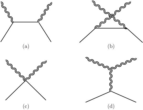
Figure 5: Diagrams relevant for gravitational Compton scattering.

The contributions from the four individual diagrams can be calculated using the graviton vertices given above and are quoted in Appendix B. Each of the four diagrams has a rather complex form. However, when added together the total again simplifies enormously. Defining the kinematic factor

$$Y={\kappa^{2}\over 8e^{4}}{p_{i}\cdot k_{i}\,p_{i}\cdot k_{f}\over k_{i}\cdot k_{f}}={\kappa^{4}\over 16e^{4}}{(s-m^{2})\,(u-m^{2})\over t}\,,$$ (70)

the sum of the four diagrams is found to be

$$\hskip-68.28644pt\big{\langle}p_{f},\epsilon_{B};k_{f},\epsilon_{f}\epsilon_{f}\,\big{|}{\rm Amp}_{\rm grav}\big{|}\,p_{i},\epsilon_{A};k_{i},\epsilon_{i}\epsilon_{i}\big{\rangle}_{S}=\sum_{i=1}^{4}{\rm Amp}\,({\rm Fig.}5(i))$$

$$= Y\times]\big{\langle}p_{f},\epsilon_{B};k_{i},\epsilon_{f}\,\big{|}{\rm Amp}_{\rm em}\big{|}\,p_{i},\epsilon_{A};k_{i},\epsilon_{i}\big{\rangle}_{S}\times\big{\langle}p_{f};k_{i},\epsilon_{f}\,\big{|}{\rm Amp}_{\rm em}\big{|}\,p_{i};k_{i},\epsilon_{i}\rangle_{S=0}\,,$$

(71)

with $S=1$, where

$$\langle p_{f};k_{i},\epsilon_{f}|{\rm Amp}_{\rm em}|p_{i};k_{i},\epsilon_{i}\rangle_{S=0}=2e^{2}\left[{\epsilon_{i}\cdot p_{i}\,\epsilon_{f}^{*}\cdot p_{f}\over p_{i}\cdot k_{i}}-{\epsilon_{i}\cdot p_{f}\,\epsilon_{f}^{*}\cdot p_{i}\over p_{i}\cdot k_{f}}-\epsilon_{f}^{*}\cdot\epsilon_{i}\right]\,,$$ (72)

is the Compton amplitude for a spinless target.

In  [8] the identity Eq. (71) was verified for simpler cases of $S=0$ and $S={1\over 2}$. This relation is a consequence of the general connections between gravity and gauge theory tree-level amplitudes derived using string-based methods as explained in [18]. Here we have demonstrated its validity for the much more complex case of spin-1 scattering. The corresponding cross-section can be calculated by helicity methods using

$$D^{1}(ab;cd)=Y\times B^{1}(ab;cd)\times A^{0}(cd)\,,$$ (73)

where $D^{1}(ab;cd)$ is the spin-1 helicity amplitude for gravitational Compton scattering, $B^{1}(ab;cd)$ is the ordinary spin-1 Compton helicity amplitude calculated in section 3, and

$$A^{0}(++) = 2e^{2}{m^{4}-su\over\big{(}s-m^{2})\big{(}u-m^{2})}\,,$$

$$A^{0}(+-) = 2e^{2}{-m^{2}t\over\big{(}s-m^{2})\big{(}u-m^{2})}\,,$$ (74)

are the helicity amplitudes for spin zero Compton scattering rising from Eq. 72 calculated in  [8]. Using Eq. (71) the invariant cross-section for unpolarized spin-1 gravitational Compton scattering

$${d\sigma^{\rm g-Comp}_{S=1}\over dt}={1\over 16\pi\big{(}s-m^{2}\big{)}^{2}}\ {1\over 3}\sum_{a=-,0,+}{1\over 2}\sum_{c=-,+}\big{|}D^{1}(ab;cd)\big{|}^{2}\,,$$ (75)

is found to be

$${d\sigma^{\rm g-Comp}_{S=1}\over dt} = {\kappa^{4}\over 768\pi\big{(}s-m^{2}\big{)}^{4}\big{(}u-m^{2}\big{)}^{2}t^{2}}\left[(m^{4}-su)^{2}\big{(}3(m^{4}-su)+t^{2})(m^{4}-su+t^{2})\big{)}\right.$$ (76)

$$+ \left.m^{4}t^{4}(3m^{2}-t)(m^{2}-t)\right]\,,$$

and this form can be compared with the unpolarized gravitational Compton cross-sections found in  [8]

$${d\sigma^{\rm g-Comp}_{S=0}\over d\Omega} = {\kappa^{4}\over 256\pi\big{(}s-m^{2}\big{)}^{4}\big{(}u-m^{2}\big{)}^{2}t^{2}}\left.\Big{[}(m^{4}-su)^{4}+m^{8}t^{4}\right.\Big{]}\,$$

$${d\sigma^{\rm g-Comp}_{S={1\over 2}}\over dt} = {\kappa^{4}\over 512\pi\big{(}s-m^{2}\big{)}^{4}\big{(}u-m^{2}t^{2}\big{)}^{2}}\left[\big{(}m^{4}-su\big{)}^{3}\big{(}2(m^{4}-su)+t^{2}\big{)}+m^{6}t^{4}\big{(}2m^{2}-t\big{)}\right]\,.$$

(77)

The corresponding laboratory frame cross-sections are

$${d\sigma_{{\rm lab},S=1}^{\rm g-Comp}\over d\Omega} = G^{2}m^{2}{\omega_{f}^{4}\over\omega_{i}^{4}}\left[\bigg{(}{\rm ctn}^{4}{\theta_{L}\over 2}\cos^{4}{\theta_{L}\over 2}+\sin^{4}{\theta_{L}\over 2}\bigg{)}\bigg{(}1+2{\omega_{i}\over m}\sin^{2}{\theta_{L}\over 2}\bigg{)}^{2}\right.$$

$$+ \left.{16\over 3}{\omega_{i}^{2}\over m^{2}}\bigg{(}\cos^{6}{\theta_{L}\over 2}+\sin^{6}{\theta_{L}\over 2}\bigg{)}\bigg{(}1+2{\omega_{i}\over m}\sin^{2}{\theta_{L}\over 2}\bigg{)}\right.$$

$$+ \left.{16\over 3}{\omega_{i}^{4}\over m^{4}}\sin^{2}{\theta_{L}\over 2}\bigg{(}\cos^{4}{\theta_{L}\over 2}+\sin^{4}{\theta_{L}\over 2}\bigg{)}\right]\,,$$

$${d\sigma^{\rm g-Comp}_{{\rm lab},S={1\over 2}}\over d\Omega} = G^{2}m^{2}{\omega_{f}^{3}\over\omega_{i}^{3}}\left[\bigg{(}{\rm ctn}^{4}{\theta_{L}\over 2}\cos^{4}{\theta_{L}\over 2}+\sin^{4}{\theta_{L}\over 2}\bigg{)}+2{\omega_{i}\over m}\bigg{(}{\rm ctn}^{2}{\theta_{L}\over 2}\cos^{6}{\theta_{L}\over 2}+\sin^{6}{\theta_{L}\over 2}\bigg{)}\right.$$

$$+ \left.2{\omega_{i}^{2}\over m^{2}}\bigg{(}\cos^{6}{\theta_{L}\over 2}+\sin^{6}{\theta_{L}\over 2}\bigg{)}\right]\,,$$

$${d\sigma^{\rm g-Comp}_{{\rm lab},S=0}\over d\Omega} = G^{2}m^{2}{\omega_{f}^{2}\over\omega_{i}^{2}}\left[{\rm ctn}^{4}{\theta_{L}\over 2}\cos^{4}{\theta_{L}\over 2}+\sin^{4}{\theta_{L}\over 2}\right]\,.\emph{}$$ (78)

We observe that the low-energy laboratory cross-section has the universal form for any spin

$${d\sigma_{{\rm lab},S}^{\rm g-Comp}\over d\Omega}=G^{2}m^{2}\left[\left({\rm ctn}^{4}{\theta_{L}\over 2}\cos^{4}{\theta_{L}\over 2}+\sin^{4}{\theta_{L}\over 2}\right)\left(1+{\cal O}\Big{(}{\omega_{i}\over m}\Big{)}\right)\right]\,.$$ (79)

It is interesting to note that the “dressing” factor for the leading $(++)$ helicity Compton amplitude—

$$\big{|}Y\big{|}\,\big{|}A^{++}\big{|}\ =\ {\kappa^{2}\over 2e^{2}}\ {m^{4}-su\over-t}\ \ \stackrel{{\scriptstyle\rm lab}}{{\longrightarrow}}\ \ {\kappa^{2}m^{2}\over 2e^{2}}\ {\cos^{2}{\theta_{L}\over 2}\over\sin^{2}{\theta_{L}\over 2}}\,,$$ (80)

—is simply the square of the photo-production dressing factor $H$, as might intuitively be expected since now both photons must be dressed in going from the Compton to the gravitational Compton cross-section. In this case the universality of the nonrelativistic cross-section follows from the leading contribution arising from the graviton pole term

$${\rm Amp}_{g-pole}\ \ \underset{\omega\ll m}{\longrightarrow}\ \ {\kappa\over 4k_{f}\cdot k_{i}}\ \big{(}\epsilon_{f}^{*}\cdot\epsilon_{i}\big{)}^{2}\ \big{(}k_{f}^{\mu}k_{f}^{\nu}+k_{i}^{\mu}k_{i}^{\nu}\big{)}\ {\kappa\over 2}\ \big{\langle}p_{f};S,M_{f}\,\big{|}T_{\mu\nu}\big{|}\,p_{i};S,M_{i}\big{\rangle}\,.$$ (82)

Here the matrix element of the energy-momentum tensor has the universal low-energy structure

$${\kappa\over 2}\,\big{\langle}p_{f};S,M_{f}\,\big{|}T_{\mu\nu}\big{|}\,p_{i};S,M_{i}\big{\rangle}={\kappa\over 4m}\,\big{(}p_{f\mu}p_{i\nu}+p_{f\nu}p_{i\mu}\big{)}\,\delta_{M_{f},M_{i}}\Big{(}1+{\cal O}\Big{(}{p_{f}-p_{i}\over m}\Big{)}\Big{)}\,,$$ (83)

where we have divided by the factor $2m$ to account for the normalization of the target particle. We find then the universal form for the leading graviton pole amplitude

$${\rm Amp}_{g-pole}\ \ \underset{\rm non-rel}{\longrightarrow}\ \ {\kappa^{2}\over 8m\,k_{f}\cdot k_{i}}\ \big{(}\epsilon_{f}^{*}\cdot\epsilon_{i}\big{)}^{2}\,\big{(}p_{i}\cdot k_{f}\,p_{f}\cdot k_{f}+p_{i}\cdot k_{i}\,p_{f}\cdot k_{i}\big{)}\,\delta_{M_{f},M_{i}}\,.$$ (84)

Since $p\cdot k\underset{\omega\ll m}{\longrightarrow}m\omega$ the helicity amplitudes become

$${\rm Amp}_{g-pole}^{\rm NR}=4\pi Gm\left\{\begin{array}[]{ll}{\big{(}1+\cos\theta_{L}\big{)}^{2}\over 2\big{(}1-\cos\theta_{L}\big{)}}={\cos^{4}{\theta_{L}\over 2}\over\sin^{2}{\theta_{L}\over 2}}&++=--\,,\\[8.61108pt] {\big{(}1-\cos\theta_{L}\big{)}^{2}\over 2\big{(}1-\cos\theta_{L}\big{)}}={\sin^{4}{\theta_{L}\over 2}\over\sin^{2}{\theta_{L}\over 2}}&+-=-+\,.\end{array}\right.$$ (87)

Squaring and averaging,summing over initial,final spins we find

$${d\sigma_{{\rm lab},S}^{\rm g-Comp}\over d\Omega}\ \ \underset{\omega\ll m}{\longrightarrow}\ \ G^{2}\,m^{2}\,\bigg{[}{\rm ctn}^{4}{\theta_{L}\over 2}\cos^{4}{\theta_{L}\over 2}+\sin^{4}{\theta_{L}\over 2}\bigg{]}\,,$$ (88)

as found in Eq. (79) above.

5 Graviton-Photon Scattering

In the previous sections we have generalized the results of  [8] to the case of a massive spin-1 target. Here we show how these spin-1 results can be used to calculate the cross-section for photon-graviton scattering. In the Compton scattering calculation we assumed that the spin-1 target had charge $e$. However, the photon couplings to the graviton are identical to those of a graviton coupled to a charged spin-1 system in the massless limit, and one might assume then that, since the results of the gravitational Compton scattering are independent of charge, the graviton-photon cross-section can be calculated by simply taking the $m\rightarrow 0$ limit of the graviton-spin-1 cross-section. Of course, the laboratory cross-section no longer makes sense since the photon cannot be brought to rest, but the invariant cross-section is well defined

$${d\sigma_{S=1}^{\rm g-Comp}\over dt}\ \ \underset{m\rightarrow 0}{\longrightarrow}\ \ {4\pi\,G^{2}\,\big{(}3s^{2}u^{2}-4t^{2}su+t^{4}\big{)}\over 3s^{2}t^{2}}={4\pi G^{2}(s^{4}+u^{4}+s^{2}u^{2})\over 3s^{2}t^{2}}\,,$$ (89)

and it might be (naively) assumed that Eq. (89) is the graviton-photon scattering cross-section. However, this is not the case and the resolution of this problem involves some interesting physics.

We begin by noting that in the massless limit the only nonvanishing helicity amplitudes are

$$D^{1}(++;++)_{m=0} = D^{1}(--;--)_{m=0}=8\pi\,G\,{s^{2}\over t}\,,$$

$$D^{1}(--;++)_{m=0} = D^{1}(++;--)_{m=0}=8\pi\,G\,{u^{2}\over t}\,,$$

$$D^{1}(00;++)_{m=0} = D^{1}(00;--)_{m=0}\ \,=8\pi\,G\,{su\over t}\,,$$ (90)

which lead to the cross-section

$${d\sigma^{\rm g-Comp}_{S=1}\over dt} = {1\over 16\pi s^{2}}\,\frac{1}{3}\,\sum_{a=+,0,-}\frac{1}{2}\sum_{c=+,-}\big{|}D^{1}(ab;cd)\big{|}^{2}$$ (91)

$$= {1\over 16\pi s^{2}}\,{1\over 3\cdot 2}\,(8\pi G)^{2}\times 2\times\left[{s^{4}\over t^{2}}+{u^{4}\over t^{2}}+{s^{2}u^{2}\over t^{2}}\right]$$ (92)

$$= {4\pi\over 3}\,G^{2}{s^{4}+u^{4}+s^{2}u^{2}\over s^{2}t^{2}}\,,$$ (93)

in agreement with Eq. (89). However, this result reveals the problem. We know that in Coulomb gauge the photon has only two transverse degrees of freedom, corresponding to positive and negative helicity—there exists no longitudinal degree of freedom. Thus the correct photon-graviton cross-section is obtained by deleting the contribution from the $D^{1}(00;++)$ and $D^{1}(00;--)$ multipoles

$${d\sigma_{g\gamma}\over dt} = {1\over 16\pi s^{2}}\,\frac{1}{3}\sum_{a=+,-}\frac{1}{2}\sum_{c=+,-}\big{|}D^{1}(ab;cd)\big{|}^{2}$$ (94)

$$= {1\over 16\pi s^{2}}\,{1\over 2\cdot 2}\,\big{(}8\pi G\big{)}^{2}\times 2\times\left[{s^{4}\over t^{2}}+{u^{4}\over t^{2}}\right]=2\pi\,G^{2}\,{s^{4}+u^{4}\over s^{2}t^{2}}\,,$$ (95)

which agrees with the value calculated via conventional methods by Skobelev [19]. Alternatively, since in the center of mass frame

$${dt\over d\Omega}={\omega_{\rm CM}\over\pi}\,,$$ (96)

we can write the center of mass graviton-photon cross-section in the form

$${d\sigma_{\rm CM}\over d\Omega}=2\,G^{2}\,\omega_{\rm CM}^{2}\left({1+\cos^{8}{\theta_{\rm CM}\over 2}\over\sin^{4}{\theta_{\rm CM}\over 2}}\right)\,,$$ (97)

again in agreement with the value given by Skobelev [19].

So what has gone wrong here? Ordinarily in the massless limit of a spin-1 system, the longitudinal mode decouples because the zero helicity spin-1 polarization vector becomes

$$\epsilon_{\mu}^{0}\ \ \underset{m\rightarrow 0}{\longrightarrow}\ \ {1\over m}\bigg{(}p,\Big{(}p+{m^{2}\over 2p}+\ldots\Big{)}\hat{z}\bigg{)}={1\over m}p_{\mu}+\Big{(}0,{m\over 2p}\hat{z}\Big{)}+\ldots$$ (98)

However, the term proportional to $p_{\mu}$ vanishes when contracted with a conserved current by gauge invariance while the term in ${m\over 2p}$ vanishes in the massless limit. Indeed that the spin-1 Compton scattering amplitude becomes gauge invariant for a massless spin-1 system can be seen from the fact that the Compton amplitude can be written as

$$\hskip-39.83368pt{\rm Amp}^{\rm Comp}_{S=1}\underset{m\rightarrow 0}{\longrightarrow}{e^{2}\over p_{i}\cdot q_{i}\,p_{i}\cdot q_{f}}\left.\bigg{[}{\rm Tr}\big{(}F_{i}F_{f}F_{A}F_{B}\big{)}+{\rm Tr}\big{(}F_{i}F_{A}F_{f}F_{B}\big{)}+{\rm Tr}\big{(}F_{i}F_{A}F_{B}F_{f}\big{)}\right.$$

$$\hskip 42.67912pt-\left.{1\over 4}\left.\Big{(}{\rm Tr}\big{(}F_{i}F_{f}\big{)}{\rm Tr}\big{(}F_{A}F_{B}\big{)}+{\rm Tr}\big{(}F_{i}F_{A}\big{)}{\rm Tr}\big{(}F_{f}F_{B}\big{)}+{\rm Tr}\big{(}F_{i}F_{B}\big{)}{\rm Tr}\big{(}F_{f}F_{A}\big{)}\right.\Big{)}\right]\,,$$

(99)

which can be checked by a bit of algebra. Equivalently, one can verify explicitly that the massless spin-1 amplitude vanishes if one replaces either $\epsilon_{A\mu}$ by $p_{i\mu}$ or $\epsilon_{B\mu}$ by $p_{f\mu}$. However, what takes place when two longitudinal spin-1 particles are present is that the product of longitudinal polarization vectors is proportional to $1/m^{2}$, while the correction term to the four-momentum $p_{\mu}$ is ${\cal O}(m^{2})$ so that the product is nonvanishing in the massless limit and this is why the multipole $D(00;++)_{m=0}=D(00;--)_{m=0}$ is nonzero. One deals with this problem by simply omitting the longitudinal degree of freedom explicitly, as done above.

5.1 Extra Credit

Before leaving this section it is interesting to note that graviton-graviton scattering can be treated in a parallel fashion. That is, the graviton-graviton scattering amplitude can be obtained by dressing the product of two massless spin-1 Compton amplitudes [20]—

$$\big{\langle}p_{f},\epsilon_{B}\epsilon_{B};k_{f},\epsilon_{f}\epsilon_{f}\,\big{|}{\rm Amp}^{\rm tot}_{grav}\big{|}\,p_{i}\epsilon_{A}\epsilon_{A};k_{i},\epsilon_{i}\epsilon_{i}\big{\rangle}_{m=0,S=2}=$$ (100)

$$Y\times\langle p_{f},\epsilon_{B};k_{f},\epsilon_{f}\,|{\rm Amp}^{\rm Comp}_{em}|\,p_{i},\epsilon_{A};k_{i}\epsilon_{i}\rangle_{m=0,S=1}\times\langle p_{f},\epsilon_{B};k_{f},\epsilon_{f}\,|{\rm Amp}^{\rm Comp}_{em}|\,p_{i},\epsilon_{A};k_{i}\epsilon_{i}\rangle_{m=0,S=1}\,.$$

Then for the helicity amplitudes we have

$$E^{2}(++;++)_{m=0}=Y\big{(}B^{1}(++;++)_{m=0}\big{)}^{2}\,,$$ (101)

where $E^{2}(++;++)$ is the graviton-graviton $++;++$ helicity amplitude while $B^{1}(++;++)$ is the corresponding spin-1 Compton helicity amplitude. Thus we find

$$E^{2}(++;++)_{m=0}={\kappa^{2}\over 16e^{4}}\,{su\over t}\times\bigg{(}{2e^{2}\,{s\over u}}\bigg{)}^{2}=8\pi\,G\,{s^{3}\over ut}\,,$$ (102)

which agrees with the result calculated via conventional methods [21].

6 The forward cross-section

It is interesting to note some intriguing physics associated with the forward-scattering limit. In this limit, i.e., $\theta_{L}\to 0$, in the laboratory frame, the Compton cross-section evaluated in section 3 has a universal structure independent of the spin $S$ of the massive target

$$\lim_{\theta_{L}\to 0}{d\sigma^{\rm Comp}_{{\rm lab},S}\over d\Omega}={\alpha^{2}\over 2m^{2}}\,,$$ (103)

reproducing the well-known Thomson scattering cross-section.

For graviton photo-production, however, the small-angle limit is very different, since the forward-scattering cross-section is divergent—the small angle limit of the graviton photo-production of section 4.1 is given by

$$\lim_{\theta_{L}\to 0}{d\sigma^{\rm photo}_{{\rm lab},S}\over d\Omega}={4G\alpha\over\theta_{L}^{2}}\,,$$ (104)

and arises from the photon pole in figure 4(d). Notice that this behavior differs from the familiar $1/\theta^{4}$ small-angle Rutherford cross-section for scattering in a Coulomb-like potential. Rather, this divergence of the forward cross-section indicates that a long range force is involved but with an effective $1/r^{2}$ potential. This effective potential arising from the $\gamma$-pole in figure 4(d), is the Fourier transform with respect to the momentum transfer $q=k_{f}-k_{i}$ of the low-energy limit given in Eq. 65. Because of the linear dependence in the momenta in the numerator, one obtains

$$\int{d^{3}q\over(2\pi)^{3}}\,e^{i\bm{q}\cdot\bm{r}}\,{1\over|\bm{q}|}={1\over 2\pi^{2}r^{2}}\,,$$ (105)

and this result is the origin of the peculiar forward-scattering behavior of the cross-section. Another contrasting feature of graviton photo-production is the independence of the forward cross-section on the mass $m$ of the target.

The small angle limit of the gravitational Compton cross-section derived in section 4.2 is given by

$$\lim_{\theta_{L}\to 0}{d\sigma^{\rm g-Comp}_{lab,S}\over d\Omega}={16G^{2}m^{2}\over\theta_{L}^{4}}\,,$$ (106)

where again the limit is independent of the spin $S$ of the matter field. Finally, the photon-graviton cross-section derived in section 5, has the forward-scattering dependence

$$\lim_{\theta_{\rm CM}\to 0}{d\sigma_{\rm CM}\over d\Omega}={32G^{2}\omega_{\rm CM}^{2}\over\theta_{\rm CM}^{4}}\,.$$ (107)

The behaviors in Eqs. (106) and (107) are due to the graviton pole in figure 5(d), and are typical of the small-angle behavior of Rutherford scattering in a Coulomb potential.

The classical bending of the geodesic for a massless particle in a Schwarzschild metric produced by a point-like mass $m$ is given by $b=4Gm/\theta+O(1)$ [22], where $b$ is the classical impact parameter. The associated classical cross-section is

$${d\sigma^{\rm classical}\over d\Omega}={b\over\sin\theta}\left|db\over d\theta\right|\simeq{16G^{2}m^{2}\over\theta^{4}}+O(\theta^{-3})\,,$$ (108)

matching the expression in Eq. (106). The diagram in Figure 5(d) describes the gravitational interaction between a massive particle of spin-$S$ and a graviton. In the forward-scattering limit the remaining diagrams of figure 5 have vanishing contributions. Since this limit is independent of the spin of the particles interacting gravitationally, the expression in Eq. (106) describes the forward gravitational scattering cross-section of any massless particle on the target of mass $m$ and explains the match with the classical formula given above.

Eq. (107) can be interpreted in a similar way, as the bending of a geodesic in a geometry curved by the energy density with an effective Schwarzschild radius of $\sqrt{2}\,G\omega_{\rm CM}$ determined by the center-of-mass energy [23]. However, the effect is fantastically small since the cross-section in Eq. (107) is of order $\ell_{P}^{4}/(\lambda^{2}\,\theta_{\rm CM}^{4})$ where $\ell_{P}^{2}=\hbar G/c^{3}\sim 1.62\,10^{-35}\,$m is the Planck length, and $\lambda$ the wavelength of the photon.

7 Bending of Light in Classical General Relativity

We close our discussion by examining the process of gravitational light bending and look at different pictures by which this phenomenon can be discussed. We begin with the standard general relaticistic derivation. The theory of general relativity encapsulates the theory of gravity in terms of a simple second rank tensor equation [24]

$$R_{\mu\nu}-{1\over 2}g_{\mu\nu}R=-{\kappa^{2}\over 4}T_{\mu\nu}\,,$$ (109)

where $\kappa^{2}=32\pi G$ is the gravitational coupling constant, $T_{\mu\nu}$ is the energy-momentum tensor,

$$g_{\mu\nu}=\eta_{\mu\nu}+h_{\mu\nu}\,,$$ (110)

is the metric tensor, and $R_{\mu\nu},\,R$ are the Ricci curvature tensor, scalar curvature, which are defined in terms of $h_{\mu\nu}$ as

$$R_{\mu\nu} = {\kappa\over 2}\left[\partial_{\mu}\partial_{\nu}h+\partial_{\lambda}\partial^{\lambda}h_{\mu\nu}-\partial_{\mu}\partial_{\lambda}{h}^{\lambda}{}_{\nu}-\partial_{\nu}\partial_{\lambda}{h}^{\lambda}{}_{\mu}\right]\,,$$

$$R = \eta^{\mu\nu}R_{\mu\nu}=\kappa\left[\Box h-\partial_{\mu}\partial_{\nu}h^{\mu\nu}\right]\,,$$ (111)

in the linear approximation. For a spatially isotropic spacetime the invariant time interval $d\tau$ is defined via a metric tensor of the form

$$d\tau^{2}=g_{\mu\nu}dx^{\mu}dx^{\nu}=A(r)dt^{2}-B(r)dr^{2}-r^{2}d\Omega^{2}\,,$$

and vanishes in the case of the motion of a massless system such as a photon. We represent the sun as a simple non-spinning massive object, described by the Schwarzschild metric [25]

$$A(r)=1-{2GM\over r},\quad B(r)={1\over 1-{2GM\over r}}\,.$$ (112)

The solution for the bending angle is then given by standard methods [24]

$$\theta=2\int_{0}^{1}{du\over\sqrt{1-u^{2}-{2GM\over D}(1-u^{3})}}-\pi\,,$$ (113)

where we have defined $u={D\over r}$. Here $D$ is the distance of closest approach in Scwarzschild coordinates. The integration in Eq. (113) can be performed exactly in terms of elliptic functions, but since near the solar rim $2GM/D\simeq 10^{-3}\ll 1$, we can instead use a perturbative solution

$$\theta = 2\int_{0}^{1}du\left[{1\over\sqrt{(1-u)(1+u)}}+{GM\over D}{1+u+u^{2}\over\sqrt{(1-u)(1+u)^{3}}}\right.$$ (114)

$$+ \left.{3\over 2}{G^{2}M^{2}\over D^{2}}{(1+u+u^{2})^{2}\over\sqrt{(1-u)(1+u)^{5}}}+\ldots\right]-\pi$$

$$= {4GM\over D}+{4G^{2}M^{2}\over D^{2}}\left({15\pi\over 16}-1\right)+\ldots$$

However, instead of using the coordinate-dependent quantity $D$, the bending angle should be written in terms of the invariant impact parameter $b$, defined as

$$b=\sqrt{B(D)}D={R\over\sqrt{1-{2GM\over D}}}=D+GM+\ldots\,,$$ (115)

we have then

$$\theta={4GM\over b}+{15\pi\over 4}{G^{2}M^{2}\over b^{2}}+\ldots\,,$$ (116)

which is the standard result, together with the next to leading order correction.

8 Quantum Mechanical Scattering Amplitude

Both alternative methods require the quantum mechanical scattering amplitude for the gravitational interaction of neutral massive and massless systems. For simplicity we take both to be spinless and therefore described by the simple Klein-Gordon Lagrangian [26]

$${\cal L}={1\over 2}\left(g^{\mu\nu}\partial_{\mu}\phi\partial_{\nu}\phi-m^{2}\phi^{2}\right)\,,$$ (117)

so that the energy-momentum tensor is given by

$$T_{\mu\nu}=\left(2{\delta\over\delta g^{\mu\nu}}-g_{\mu\nu}\right)\sqrt{-{\rm det}g}{\cal L}=\partial_{\mu}\phi\partial_{\nu}\phi-{1\over 2}\eta_{\mu\nu}\left(\partial_{\alpha}\phi\partial^{\alpha}\phi-m^{2}\phi^{2}\right)+\ldots$$ (118)

The corresponding matrix element is then

$$<p_{f}|T_{\mu\nu}|p_{i}>=p_{f\mu}p_{i\nu}+p_{i\mu}p_{f\nu}-\eta_{\mu\nu}(p_{f}\cdot p_{i}-m^{2})+\ldots$$ (119)

Using the gravitational interaction [27]

$${\cal L}_{int}={\kappa\over 2}h^{\mu\nu}T_{\mu\nu}\,,$$ (120)

and the harmonic gauge graviton propagator

$$D_{F}^{\alpha\beta;\gamma\delta}(q)={iP^{\alpha\beta;\gamma\delta}\over q^{2}}\,,$$ (121)

where $P^{\alpha\beta;\gamma\delta}={1\over 2}(\eta^{\alpha\gamma}\eta^{\beta\delta}+\eta^{\alpha\delta}\eta^{\beta\gamma}-\eta^{\alpha\beta}\eta^{\gamma\delta})$, the lowest order graviton exchange amplitude for interaction between massive and massless systems described via initial, final energy-momentum $P_{i},\,P_{f}$ and $p_{i},\,p_{f}$ respectively, becomes (cf. Figure 1)

$$i{\cal M}_{0}(q) = {1\over\sqrt{4E_{f}E_{i}}}{1\over\sqrt{4\epsilon_{f}\epsilon_{i}}}{\kappa\over 2}<P_{f}|T_{\alpha\beta}|P_{i}>D_{F}^{\alpha\beta;\gamma\delta}(q){\kappa\over 2}<p_{f}|T_{\gamma\delta}|p_{i}>$$ (122)

$$= {\kappa^{2}\over 4}\left({s^{2}-2s(m^{2}+M^{2})+m^{4}+M^{4}\over q^{2}}+s-M^{2}-m^{2}\right)\,,$$

where $s=(P_{i}+p_{i})^{2}=(P_{f}+p_{f})^{2}$, $q^{2}=(P_{f}-P_{i})^{2}=(p_{f}-p_{i})^{2}$, and we have divided by the conventional normalizing factors $\sqrt{2E}$ for each external scalar field. Working in the rest frame of the system having mass $M$, if the light system has mass $m$, then in the nonrelativistic limit $s\simeq(M+m)^{2}$ and $q_{0}\simeq 0$ so that

$${\cal M}_{0}(\bm{q})\simeq-{1\over 4Mm}{\kappa^{2}\over 4}{2M^{2}m^{2}\over\bm{q}^{2}}=-{4\pi GMm\over\bm{q}^{2}}\,.$$ (123)

In Born approximation the transition amplitude is related to the potential via [28]

$${\cal M}_{0}(\bm{q})=<\bm{p}_{f}|\hat{V}_{0}|\bm{p}_{i}>=\int d^{3}re^{i\bm{q}\cdot\bm{r}}V_{0}(\bm{r})\,,$$ (124)

where $\bm{q}=\bm{p}_{i}-\bm{p}_{f}$. The corresponding gravitational potential is then given by the inverse Fourier transform

$$V_{0}(r)=\int{d^{3}q\over(2\pi)^{3}}e^{-i\bm{q}\cdot\bm{r}}{\cal M}_{0}(\bm{q})=-{GMm\over r}\,,$$ (125)

and has the expected Newtonian form. However, if the light system is massless and carries energy $E_{m}$, then $s=M^{2}+2ME_{m}$ so that

$${\cal M}_{0}(q)\simeq-{8\pi GME_{m}\over\bm{q}^{2}}\,.$$ (126)

and the gravitational potential becomes

$$V_{0}(r)=\int{d^{3}q\over(2\pi)^{3}}e^{-i\bm{q}\cdot\bm{r}}{\cal M}_{0}(\bm{q})=-{2GME_{m}\over r}$$ (127)

Higher order corrections to this lowest order potential can be found by calculating loop effects. Such calculations have been performed by a number of groups and the next to leading order (${\cal O}(G^{2})$) form of the gravitational interaction amplitude has been found to be [30]

$${\cal M}_{1}(q)=-{15\pi^{2}G^{2}M^{2}E_{m}\over 2\sqrt{\bm{q}^{2}}}+\ldots\,,$$ (128)

which will be used below. With these forms in hand, we can now proceed to alternative light bending calculations.

9 Geometrical Optics

In section 7 we presented the conventional (particle) derivation of the bending angle, in terms of the trajectory traveled by photons. In this section we review an alternative approach, presented in [9], to describe the propagation of light via geometrical optics, wherein the beam travels through a region defined by a position-dependent index of refraction $n(r)$, in which case we have the equation of motion [31]

$${d\over ds}n{d\bm{r}\over ds}=\bm{\nabla}n\,,$$ (129)

where $\bm{r}(s)$ is the trajectory as a function of the path length $s$. In the case of light $ds\simeq cdt$ and Eq. (129) simplifies to

$${1\over c^{2}}{d^{2}\bm{r}\over dt^{2}}={1\over n}\bm{\nabla}n\,.$$ (130)

The index of refraction describes the propagation of light when $E\neq|\bm{p}|$, and is defined by $n=E/|\bm{p}|$. In our case, as discussed in the previous section, the presence of the gravitational interaction between photons and the sun leads to a modification of the energy and therefore to an effective position dependent index of refraction

$$n(r)\simeq(E_{m}-V(r))/E_{m}=1-{1\over E_{m}}V(r)\,.$$ (131)

where, for a massless scalar with energy $E_{m}$ interacting with a mass $M$ we found

$$V_{0}(r)=-{2GME_{m}\over r}$$ (133)

In the absence of a potential ($n(r)=1$) consider a light beam incident along the $\hat{\bm{e}}_{y}$ direction and with impact parameter $b$ on a massive target located at the origin. The trajectory is then characterized by the straight line

$$\bm{r}_{0}(t)=b\hat{\bm{e}}_{x}+ct\hat{\bm{e}}_{y},\qquad-\infty<t<\infty.$$ (134)

If we now turn on a potential $V_{0}(r)$ the index of refraction is no longer unity and there will exist a small deviation from this straight line trajectory. Integrating Eq. (130) we find

$$\Delta{1\over c^{2}}{d\bm{r}\over dt}=-{1\over E_{m}}\int_{-\infty}^{\infty}dt\bm{\nabla}V_{0}(r)=-{1\over E_{m}}\int_{-\infty}^{\infty}dtV_{0}^{\prime}(r)\hat{\bm{r}}\,,$$ (135)

so that

$${1\over c}\theta\simeq{1\over E_{m}}\int_{-\infty}^{\infty}dtV_{0}^{\prime}(\sqrt{b^{2}+c^{2}t^{2}}){b\over\sqrt{b^{2}+c^{2}t^{2}}}\,,$$ (136)

where $\theta$ is the bending angle. Now change variables to $t=bu/c$, yielding

$${1\over c}\theta\simeq{b\over E_{m}}\int_{-\infty}^{\infty}duV_{0}^{\prime}(b\sqrt{1+u^{2}}){1\over\sqrt{1+u^{2}}}\,.$$ (137)

That is,

$$\theta_{0}={b\over E_{m}}\int_{\infty}^{\infty}{du\over\sqrt{1+u^{2}}}V_{0}^{\prime}(b\sqrt{1+u^{2}})={b\over E_{m}}\int_{-\infty}^{\infty}{2GE_{m}Mdu\over b^{2}(1+u^{2})^{3\over 2}}={4GM\over b}\,,$$ (138)

as expected.

The leading correction to Eq. 138 arises from the one-loop correction to the potential discussed above

$$V_{1}(r)=-\int{d^{3}q\over(2\pi)^{3}}e^{-i\bm{q}\cdot\bm{r}}{15\pi^{2}G^{2}M^{2}E_{m}\over 2\sqrt{\bm{q}^{2}}}=-{15G^{2}M^{2}E_{m}\over 4r^{2}}\,,$$ (139)

so the additional bending is given by

$$\theta_{1}={b\over E_{m}}\int_{-\infty}^{\infty}{du\over\sqrt{1+u^{2}}}V_{1}^{\prime}(b\sqrt{1+u^{2}})={b\over E_{m}}\int_{-\infty}^{\infty}{15G^{2}M^{2}E_{m}du\over 2b^{3}(1+u^{2})^{2}}={15\pi G^{2}M^{2}\over 4b^{2}}\,,$$ (140)

in agreement with the result found by the conventional GR method. We see then that geometrical optics, in which light is treated in a wavelike fashion, provides and interesting alternative way to look at the bending process.

10 Small-Angle Scattering (Eikonal) Method

A third approach, , discussed in [9], is to look at the bending in terms of a particle interpretation but using quantum mechanics rather than classical physics. In this method we consider a trajectory in terms of a series of small angle high energy scatterings of the photons by the sun. In such a situation the dominant four-momentum transfer is in the transverse spatial directions. For photons travelling in the $z$-direction we have $p_{3}=p_{1}+q$, so that, squaring, we obtain $0=2E(q_{0}-q_{z})+q^{2}$. A similar calculation for the heavy mass gives $0=-2Mq_{0}+q^{2}$, which tells us that both $q_{\pm}=q_{0}\pm q_{z}$ are suppressed compared to the transverse components $q^{2}\sim-\bm{q}^{2}_{\perp}$ by at least a factor of $2E$. This condition on the overall momentum transfer gets reflected in the same stricture for the exchanged gravitons, so that the dominant momentum transfer inside loops is also transverse. (In the effective theory of high energy scattering—Soft Collinear Effective Theory (SCET)—these are called Glauber modes and carry momentum scaling $(k_{+},k_{-},k_{\bot})\sim\sqrt{s}(\lambda^{2},\lambda^{2},\lambda)$ where $\lambda\sim\sqrt{-t/s}$ [34].)

The one-graviton amplitude amplitude in this limit was found above to be

$${\cal M}_{0}(\bm{q}_{\perp})=-\kappa^{2}M^{2}E^{2}\frac{1}{\bm{q}_{\perp}^{2}}\,.$$ (141)

After some work described in Appendix B, the multiple graviton exchanges of this amplitude can be summed, yielding

$${\cal M}^{(1)}_{tot}(\bm{q}_{\perp})=(4\pi)^{2}ME_{m}\sum_{n}\frac{1}{n!}\left({i\over 4}\kappa^{2}ME_{m}\right)^{n}\prod_{i=1}^{n}\int\frac{d^{2}\ell_{i}}{(2\pi)^{2}}\frac{1}{\bm{\ell}_{i}^{2}}\delta^{2}(\sum_{j=1}^{n}\bm{\ell}_{j}-\bm{q}_{\perp})\,,$$ (142)

In order to bring this amplitude into impact parameter space, one defines the two-dimensional Fourier transform, with impact parameter $\bm{b}$ being transverse to the initial motion.

$${\cal M}_{tot}(\bm{b})=\int\frac{d^{2}q_{\perp}}{(2\pi)^{2}}e^{i\bm{q}_{\perp}\cdot\bm{b}}~{}{\cal M}^{(1)}_{tot}(\bm{q}_{\perp})\,.$$ (143)

We find then

$${\cal M}_{tot}(\bm{b})=4ME_{m}\sum_{n=1}^{\infty}{1\over n!}(i\chi_{0}(\bm{b}))^{n}=2(s-M^{2})\left(e^{i\chi_{0}(\bm{b})}-1\right)\,,$$ (144)

where $\chi_{0}(\bm{b})$ is the transverse Fourier transform of the one graviton exchange amplitude

$$\chi_{0}(\bm{b}) =\frac{1}{4ME_{m}}\int\frac{d^{2}q_{\perp}}{(2\pi)^{2}}~{}e^{i\bm{q}_{\perp}\cdot\bm{b}}~{}{\cal M}_{0}(\bm{q}_{\perp})\ \$$

$$=-\frac{\kappa^{2}ME_{m}}{4}\int\frac{d^{2}q_{\perp}}{(2\pi)^{2}}~{}e^{i\bm{q}_{\perp}\cdot\bm{b}}\frac{1}{\bm{q}_{\perp}^{2}}\ \$$

$$=-4\kappa^{2}ME_{m}\left[\frac{1}{d-4}-\log b+...\right]\ \ .$$ (145)

Only the $\log b$ term will be important in calculating the bending angle. If we now transform back to momentum transfer space via

$${\cal M}_{tot}(\bm{q}_{\perp})=\int{d^{2}b\over(2\pi)^{2}}e^{-i\bm{q}_{\perp}\cdot\bm{b}}{\cal M}_{tot}(\bm{b})\,,$$ (146)

and perform the impact parameter space integration via stationary phase methods, we find

$$\frac{\partial}{\partial b}\left(|\bm{q}_{\perp}|b-\chi_{0}(b)\right)=0\,.$$ (147)

Since $|\bm{q}_{\perp}|=2E_{m}\sin\frac{\theta}{2}\simeq E_{m}\theta$ we find

$$\theta_{0}=\frac{1}{E_{m}}\frac{\partial}{\partial b}\chi_{0}(b)\,,$$ (148)

which yields the lowest order result

$$\theta_{0}={4GM\over b}\,.$$ (149)

At next to leading order we require the eikonal phase found from the one-loop correction to massive-massless scattering

$$\chi_{1}(b) = \frac{1}{4ME_{m}}\int\frac{d^{2}q_{\perp}}{(2\pi)^{2}}~{}e^{i\bm{q}_{\perp}\cdot\bm{b}}~{}{\cal M}_{1}(\bm{q}_{\perp})$$ (150)

$$= -\int{d^{2}q_{\perp}\over(2\pi)^{2}}e^{i\bm{q}_{\perp}\cdot\bm{b}}{15\pi^{2}G^{2}M^{2}E_{m}\over 2|\bm{q}_{\perp}|}=-{15\pi\over 4b}G^{2}M^{2}E_{m}\,.$$

The stationary phase calculation then yields the correction

$$\theta_{1}=\frac{1}{E_{m}}\frac{\partial}{\partial b}\chi_{1}(b)={15\pi G^{2}M^{2}\over 4b^{2}}\,,$$ (151)

which once again agrees with the classical result.

11 Conclusion

In [8] it was demonstrated that the gravitational interaction of a charged spin-0 or spin-$\frac{1}{2}$ particle is greatly simplified by use of factorization, which asserts that the gravitational amplitudes can be written as the product of corresponding electromagnetic amplitudes multiplied by a universal kinematic factor. In the present work we demonstrated that the same simplification applies when the target particle carries spin-1. Specifically, we evaluated the graviton photo-production and graviton Compton scattering amplitudes explicitly using direct and factorized techniques and demonstrated that they are identical. However, the factorization methods are enormously simpler, since they require only electromagnetic calculations and eliminate the need to employ less familiar and more cumbersome tensor quantities. As a result it is now straightforward to include graviton interactions in a quantum mechanics course in order to stimulate student interest and allowing access to various cosmological applications.

We studied the massless limit of the spin-1 system and showed how the use of factorization permits a relatively simple calculation of graviton-photon scattering, discussing a subtlety in this graviton-photon calculation having to do with the feature that the spin-1 system must change from three to two degrees of freedom when $m\rightarrow 0$ and we explained why the zero mass limit of the spin-1 gravitational Compton scattering amplitude does not correspond to that for photon scattering. The graviton-photon cross section may possess interesting implications for the attenuation of gravitational waves in the cosmos [35]. We also calculated the graviton-graviton scattering amplitude.

We discussed the main features of the forward cross-section for each process studied in this paper. Both the Compton and the gravitational Compton scattering have the expected $1/\theta_{L}^{4}$ behavior, while graviton photo-production has a different shape that could in principle lead to an interesting new experimental signature of a graviton scattering on matter—$\sim 1/\theta_{L}^{2}$. Again this result has potentially intriguing implications for the photo-production of gravitons from stars [36, 37].

Finally, we have reviewed the evaluation of the classical general relativity contribution to the light bending problem—the deviation angle occurring during the passage of a photon by the rim of the sun—in three different ways. The result in each case was found to be identical

$$\theta={4GM\over b}+{15\pi G^{2}M^{2}\over 4b^{2}}+\ldots$$ (152)

What is interesting about these results is that they were obtained using apparently very disparate pictures.

• In the first, light is considered from the point of view of photons traversing a classical trajectory in the vicinity of a massive object.

• In the second, the propagation of light is determined by standard geometrical optics, in the presence of an effective index of refraction determined by the effective potential describing the gravitational interaction of massive and massless systems.

• Finally, in the third, standard quantum mechanical scattering methods were used, relating the massive-massless scalar gravitational interaction to the eikonal phase associated with a series of small-angle scatterings.

In the latter two cases, it may seem surprising that a method based on a three dimensional Fourier transform, yielding an effective index of refraction, yields results identical to those obtained using small angle scattering theory, involving a two-dimensional eikonal Fourier transform. However, the equivalence is shown in Appendix A to result from a simple mathematical identity. What we hope results from this comparison of the various methods is a deeper understanding and illumination of an important general relativistic phenomenon—that of light bending in the presence of a gravitational field.

We close by noting that the same method permits the determination of a quantum effect in the bending angle, with the result [38] (and [39])

$$\theta_{S}=\left(8bu^{S}+9-48\log{b\over 2b_{0}}\right)\,{\hbar G_{N}^{2}M\over\pi b^{3}}\,,$$ (153)

where $bu^{S}$ is a coefficient that depend on the spin $S$ of the massless particle scattered against the mass stellar object $M$. The spin dependence of the quantum raises questions about the interpretation of the equivalence principle at the quantum mechanical level [40, 38, 9] and strongly suggests additional investigations concerning the nature of the Equivalence principle at the quantum level that we leave for future work.

Appendix A Equivalence between eikonal and geometrical optics

In order to provide a general proof of the equivalence between eikonal and geometrical optics methods, we note that the eikonal phase is, in general, given by

$$\chi(b)=\int{d^{2}q_{\perp}\over(2\pi)^{2}}e^{-i\bm{q}_{\perp}\cdot\bm{b}}{\rm Amp}(\bm{q}_{\perp}^{2})={1\over 2\pi}\int_{0}^{\infty}dssJ_{0}(b|\bm{s}|){\rm Amp}(\bm{s}^{2})\,,$$ (154)

where ${\rm Amp}(s^{2})$ is the photon-mass scattering amplitude. The corresponding contribution to the lightbending angle is then

$$\theta={1\over E_{m}}{d\over db}\chi(b)=-{1\over 2\pi E_{m}}\int_{0}^{\infty}dss^{2}J_{1}(b|\bm{s}|){\rm Amp}(\bm{s}^{2})\,,$$ (155)

where we have used $J_{0}^{\prime}(x)=-J_{1}(x)$.

On the other hand, in the geometrical optics method, we use the three-dimensional Fourier transform

$$V(r)=\int{d^{3}q\over(2\pi)^{3}}e^{-i\bm{q}\cdot\bm{r}}{\rm Amp}(\bm{q}^{2})={1\over 2\pi^{2}}\int_{0}^{\infty}dqq^{2}j_{0}(|\bm{q}|r){\rm Amp}(\bm{q}^{2})\,,$$ (156)

in terms of which the lightbending shift is

$$\theta=-{b\over 2\pi^{2}E_{m}}\int_{-\infty}^{\infty}{du\over\sqrt{1+u^{2}}}\int_{0}^{\infty}dqq^{3}j_{1}(|\bm{q}|b\sqrt{1+u^{2}}){\rm Amp(\bm{q}^{2})}\,,$$ (157)

where we have noted $j_{0}^{\prime}(x)=-j_{1}(x)$. Using $j_{1}(x)=\sqrt{\pi\over 2x}J_{3\over 2}(x)$ we have

$$\theta=-{b\over 2\pi^{2}E_{m}}\int_{0}^{\infty}dqq^{3}G(|\bm{q}|b){\rm Amp(\bm{q}^{2})}\,,$$ (158)

where

$$G(|\bm{q}|b)=\sqrt{\pi\over 2|\bm{q}|b}\int_{-\infty}^{\infty}{du\over(1+u^{2})^{3\over 4}}J_{3\over 2}(|\bm{q}|b\sqrt{1+u^{2}})\,.$$ (159)

Changing variables to $s=\sqrt{1+u^{2}}$ so $u=\sqrt{s^{2}-1}$, then $du=sds/\sqrt{s^{2}-1}$ and

$$G(|\bm{q}|b)=\sqrt{\pi\over 2|\bm{q}|b}\int_{-\infty}^{\infty}{ds\over\sqrt{s(s^{2}-1)}}J_{3\over 2}(|\bm{q}|bs)\,.$$ (160)

We have [41]

$$\int_{0}^{\infty}{dxJ_{3\over 2}(sx)\over\sqrt{x(x^{2}-1)}}=\sqrt{\pi\over 2s}(J_{1}(s)-iL_{1}(-is))\,,$$ (161)

where $L_{1}(x)$ is a modified Struve function and satisfies $L_{1}(x)=L_{1}(-x)$ while $J_{1}(x)=-J_{1}(-x)$ is the usual Bessel function. . If then we change the integration to the range $-\infty$ to $\infty$, the Struve function disappears and we have

$$G(|\bm{q}|b)=\sqrt{\pi\over 2|\bm{q}|b}\cdot\sqrt{2\pi\over|\bm{q}|b}J_{1}(|\bm{q}|b)={\pi\over|\bm{q}|b}J_{1}(|\bm{q}|b)\,,$$ (162)

whereby

$$\theta=-{1\over 2\pi E_{m}}\int_{0}^{\infty}dqq^{2}J_{1}(|\bm{q}|b){\rm Amp}(\bm{q}^{2}),$$ (163)

which is identical to the eikonal result.

Appendix B Graviton Scattering Amplitudes

In this appendix we list the independent contributions to the various graviton scattering amplitudes which must be added in order to produce the complete and gauge invariant amplitudes quoted in the text. We leave it to the (perspicacious) reader to perform the appropriate additions and to verify the equivalence of the factorized forms shown earlier.

B.1 Graviton Photo-production: spin-1

For the case of graviton photoproduction, we find the four contributions, cf. Fig. 4,

$$\!\!\!\!\!\!\!\!\!\!\!\!\!\!\!\!{\rm Fig.4(a)}: \!\!\!\!\!\!\!\!\!{{\rm Amp}_{a}(S=1)}={\kappa e\over p_{i}\cdot k_{i}}\,\bigg{(}\epsilon_{i}\cdot p_{i}\Big{[}\epsilon_{B}^{*}\cdot\epsilon_{A}\,\epsilon_{f}^{*}\cdot p_{f}\,\epsilon_{f}^{*}\cdot p_{f}-\epsilon_{B}^{*}\cdot k_{f}\,\epsilon_{f}^{*}\cdot p_{f}\,\epsilon_{f}^{*}\cdot\epsilon_{A}$$ (164)

$$- \epsilon_{A}\cdot p_{f}\,\epsilon_{f}^{*}\cdot p_{f}\,\epsilon_{f}^{*}\cdot\epsilon_{B}^{*}+p_{f}\cdot k_{f}\,\epsilon_{f}^{*}\cdot\epsilon_{A}\,\epsilon_{f}^{*}\cdot\epsilon_{B}^{*}\Big{]}$$

$$+ \epsilon_{A}\cdot\epsilon_{i}\Big{[}\epsilon_{B}^{*}\cdot k_{i}\,\epsilon_{f}^{*}\cdot p_{f}\,\epsilon_{f}^{*}\cdot p_{f}-\epsilon_{B}^{*}\cdot k_{f}\,\epsilon_{f}^{*}\cdot p_{f}\,\epsilon_{f}^{*}\cdot k_{i}-p_{f}\cdot k_{i}\,\epsilon_{f}^{*}\cdot p_{f}\,\epsilon_{f}^{*}\cdot\epsilon_{B}^{*}$$

$$+ p_{f}\cdot k_{f}\,\epsilon_{f}^{*}\cdot k_{i}\,\epsilon_{f}^{*}\cdot\epsilon_{B}^{*}\Big{]}$$

$$- \epsilon_{A}\cdot k_{i}\,\Big{[}\epsilon_{B}^{*}\cdot\epsilon_{i}\,\epsilon_{f}^{*}\cdot p_{f}\,\epsilon_{f}^{*}\cdot p_{f}-\epsilon_{B}^{*}\cdot k_{f}\,\epsilon_{f}^{*}\cdot p_{f}\,\epsilon_{f}^{*}\cdot\epsilon_{i}-\epsilon_{i}\cdot p_{f}\,\epsilon_{f}^{*}\cdot p_{f}\,\epsilon_{f}^{*}\cdot\epsilon_{B}^{*}$$

$$+ p_{f}\cdot k_{f}\,\epsilon_{f}^{*}\cdot\epsilon_{i}\,\epsilon_{f}^{*}\cdot\epsilon_{B}^{*}\Big{]}$$

$$- \epsilon_{B}^{*}\cdot\epsilon_{f}^{*}\,\epsilon_{A}\cdot\epsilon_{i}\,\epsilon_{f}^{*}\cdot p_{f}p_{i}\cdot k_{i}\bigg{)}\,.$$

$$\!\!\!\!\!\!\!\!\!\!\!\!\!\!\!\!{\rm Fig.4(b)}: \!\!\!\!\!\!\!\!\!{{\rm Amp}_{b}(S=1)}=-{\kappa e\over p_{i}\cdot k_{f}}\,\bigg{(}\epsilon_{i}\cdot p_{f}\Big{[}\epsilon_{A}\cdot\epsilon_{B}^{*}\,\epsilon_{f}^{*}\cdot p_{i}\,\epsilon_{f}^{*}\cdot p_{i}-\epsilon_{B}^{*}\cdot p_{i}\,\epsilon_{f}^{*}\cdot p_{i}\,\epsilon_{f}^{*}\cdot\epsilon_{A}$$ (165)

$$+ \epsilon_{A}\cdot k_{f}\,\epsilon_{f}^{*}\cdot p_{i}\,\epsilon_{f}^{*}\cdot\epsilon_{B}^{*}-p_{i}\cdot k_{f}\,\epsilon_{f}^{*}\cdot\epsilon_{A}\,\epsilon_{f}^{*}\cdot\epsilon_{B}^{*}\Big{]}$$

$$+ \epsilon_{B}^{*}\cdot k_{i}\Big{[}\epsilon_{A}\cdot\epsilon_{i}\,\epsilon_{f}^{*}\cdot p_{i}\,\epsilon_{f}^{*}\cdot p_{i}-\epsilon_{i}\cdot p_{i}\,\epsilon_{f}^{*}\cdot p_{i}\,\epsilon_{f}^{*}\cdot\epsilon_{A}+\epsilon_{A}\cdot k_{f}\,\epsilon_{f}^{*}\cdot p_{i}\,\epsilon_{f}^{*}\cdot\epsilon_{i}$$

$$- p_{i}\cdot k_{f}\,\epsilon_{f}^{*}\cdot\epsilon_{A}\,\epsilon_{f}^{*}\cdot\epsilon_{i}\Big{]}$$

$$+ \epsilon_{i}\cdot\epsilon_{B}^{*}\Big{[}\epsilon_{A}\cdot k_{i}\,\epsilon_{f}^{*}\cdot p_{i}\,\epsilon_{f}^{*}\cdot p_{i}-p_{i}\cdot k_{i}\,\epsilon_{f}^{*}\cdot p_{i}\,\epsilon_{f}^{*}\cdot\epsilon_{A}+\epsilon_{A}\cdot k_{f}\,\epsilon_{f}^{*}\cdot p_{i}\,\epsilon_{f}^{*}\cdot k_{i}$$

$$- p_{i}\cdot k_{f}\,\epsilon_{f}^{*}\cdot\epsilon_{A}\,\epsilon_{f}^{*}\cdot k_{i}\Big{]}$$

$$- \epsilon_{A}\cdot\epsilon_{f}^{*}\,\epsilon_{f}^{*}\cdot p_{i}\,\epsilon_{B}^{*}\cdot\epsilon_{i}\,p_{i}\cdot k_{f}\bigg{)}\,.$$

$${\rm Fig.4(c)}: \!\!\!\!\!\!\!\!\!{\rm Amp}_{c}(S=1)=\kappa\,e\bigg{(}\epsilon_{f}^{*}\cdot\epsilon_{i}(\epsilon_{B}^{*}\cdot\epsilon_{A}\,\epsilon_{f}^{*}\cdot(p_{f}+p_{i})-\epsilon_{A}\cdot p_{f}\,\epsilon_{B}^{*}\cdot\epsilon_{f}^{*}-\epsilon_{B}^{*}\cdot p_{i}\,\epsilon_{A}\cdot\epsilon_{f}^{*})$$ (166)

$$- \epsilon_{B}^{*}\cdot\epsilon_{f}^{*}\,\epsilon_{A}\cdot\epsilon_{i}\,\epsilon_{f}^{*}\cdot p_{i}-\epsilon_{A}\cdot\epsilon_{f}^{*}\,\epsilon_{B}^{*}\cdot\epsilon_{i}\,\epsilon_{f}^{*}\cdot p_{f}+\epsilon_{f}^{*}\cdot\epsilon_{A}\,\epsilon_{f}^{*}\cdot\epsilon_{B}^{*}\,\epsilon_{i}\cdot(p_{f}+p_{i})\bigg{)}\,,$$

and finally, the photon pole contribution

$$\!\!\!\!\!\!\!\!\!\!\!\!\!\!\!\!\!\!\!\!\!\!\!\!\!\!\!\!\!\!\!\!\!\!\!\!\!\!\!\!\!\!\!\!\!\!\!\!\!\!\!\!\!\!\!\!\!\!\!\!\!\!\!\!\!\!\!\!\!\!\!\!\!\!\!\!\!\!\!\!\!\!\!\!\!\!\!\!\!{\rm Fig.4(d)}: \!\!\!\!{{\rm Amp_{d}}(S=1)}=-{e\,\kappa\over 2k_{f}\cdot k_{i}}$$ (167)

$$\times \bigg{[}\epsilon_{B}^{*}\cdot\epsilon_{A}\Big{[}\epsilon_{f}^{*}\cdot(p_{f}+p_{i})(k_{f}\cdot k_{i}\epsilon_{f}^{*}\cdot\epsilon_{i}-\epsilon_{f}^{*}\cdot k_{i}\,\epsilon_{i}\cdot k_{f})$$

$$+ \epsilon_{f}^{*}\cdot k_{i}(\epsilon_{f}^{*}\cdot\epsilon_{i}\,k_{i}\cdot(p_{i}+p_{f})-\epsilon_{f}^{*}\cdot k_{i}\epsilon_{i}\cdot(p_{f}+p_{i}))\Big{]}$$

$$- 2\epsilon_{B}^{*}\cdot p_{i}\Big{[}\epsilon_{f}^{*}\cdot\epsilon_{A}\,(k_{f}\cdot k_{i}\,\epsilon_{f}^{*}\cdot\epsilon_{i}-\epsilon_{f}^{*}\cdot k_{i}\,\epsilon_{i}\cdot k_{f})$$

$$+ \epsilon_{f}^{*}\cdot k_{i}\,(\epsilon_{f}^{*}\cdot\epsilon_{i}\,\epsilon_{A}\cdot k_{i}-\epsilon_{f}^{*}\cdot k_{i}\,\epsilon_{i}\cdot\epsilon_{A})\Big{]}$$

$$- 2\epsilon_{A}\cdot p_{f}\Big{[}\epsilon_{f}^{*}\cdot\epsilon_{B}^{*}(k_{f}\cdot k_{i}\,\epsilon_{f}^{*}\cdot\epsilon_{i}-\epsilon_{f}^{*}\cdot k_{i}\,\epsilon_{i}\cdot k_{f})$$

$$+ \epsilon_{f}^{*}\cdot k_{i}\,(\epsilon_{f}^{*}\cdot\epsilon_{i}\,\epsilon_{B}^{*}\cdot k_{i}-\epsilon_{f}^{*}\cdot k_{i}\,\epsilon_{i}\cdot\epsilon_{B}^{*})\Big{]}\bigg{]}\,.$$

B.2 Gravitational Compton Scattering: spin-1

In the case of gravitational Compton scattering—Figure 5—we have the four contributions

$${\rm Fig.5(a)}: {\rm Amp}_{a}(S=1)=\kappa^{2}\,{1\over 2p_{i}\cdot k_{i}}\bigg{[}(\epsilon_{i}\cdot p_{i})^{2}(\epsilon_{f}^{*}\cdot p_{f})^{2}\epsilon_{A}\cdot\epsilon_{B}^{*}$$

$$-(\epsilon_{f}^{*}\cdot p_{f})^{2}\epsilon_{i}\cdot p_{i}(\epsilon_{A}\cdot k_{i}\epsilon_{B}^{*}\cdot\epsilon_{i}+\epsilon_{A}\cdot\epsilon_{i}\,\epsilon_{B}^{*}\cdot p_{i})$$

$$-(\epsilon_{i}\cdot p_{i})^{2}\epsilon_{f}^{*}\cdot p_{f}\,(\epsilon_{B}^{*}\cdot\epsilon_{f}^{*}\,\epsilon_{A}\cdot p_{f}+\epsilon_{B}^{*}\cdot k_{f}\,\epsilon_{A}\cdot\epsilon_{f}^{*})$$

$$+\epsilon_{i}\cdot p_{i}\,\epsilon_{f}^{*}\cdot p_{f}\,\epsilon_{i}\cdot p_{f}\,\epsilon_{A}\cdot k_{i}\,\epsilon_{B}^{*}\cdot\epsilon_{f}^{*}+\epsilon_{i}\cdot p_{i}\,\epsilon_{f}^{*}\cdot p_{f}\,\epsilon_{f}^{*}\cdot p_{i}\,\epsilon_{A}\cdot\epsilon_{i}\,\epsilon_{B}^{*}\cdot k_{f}$$

$$+(\epsilon_{f}^{*}\cdot p_{f})^{2}\epsilon_{B}^{*}\cdot\epsilon_{i}\,\epsilon_{A}\cdot\epsilon_{i}\,p_{i}\cdot k_{i}+(\epsilon_{i}\cdot p_{i})^{2}\epsilon_{B}^{*}\cdot\epsilon_{f}^{*}\,\epsilon_{A}\cdot\epsilon_{f}^{*}\,p_{f}\cdot k_{f}$$

$$+\epsilon_{i}\cdot p_{i}\,\epsilon_{f}^{*}\cdot p_{f}\,(\epsilon_{A}\cdot k_{i}\,\epsilon_{B}^{*}\cdot k_{f}\,\epsilon_{i}\cdot\epsilon_{f}^{*}+\epsilon_{B}^{*}\cdot\epsilon_{f}^{*}\,\epsilon_{A}\cdot\epsilon_{i}\,p_{i}\cdot p_{f})$$

$$-\epsilon_{i}\cdot p_{i}\,\epsilon_{f}^{*}\cdot p_{i}\,\epsilon_{B}^{*}\cdot\epsilon_{f}^{*}\,\epsilon_{A}\cdot\epsilon_{i}\,p_{f}\cdot k_{f}-\epsilon_{f}^{*}\cdot p_{f}\,\epsilon_{i}\cdot p_{f}\,\epsilon_{A}\cdot\epsilon_{i}\,\epsilon_{B}^{*}\cdot\epsilon_{f}^{*}\,p_{i}\cdot k_{i}$$

$$-\epsilon_{i}\cdot p_{i}\,\epsilon_{A}\cdot k_{i}\,\epsilon_{B}^{*}\cdot\epsilon_{f}^{*}\,\epsilon_{f}^{*}\cdot\epsilon_{i}\,p_{f}\cdot k_{f}-\epsilon_{f}^{*}\cdot p_{f}\,\epsilon_{B}^{*}\cdot k_{f}\,\epsilon_{A}\cdot\epsilon_{i}\,\epsilon_{i}\cdot\epsilon_{f}^{*}\,p_{i}\cdot k_{i}$$

$$+\epsilon_{A}\cdot\epsilon_{i}\,\epsilon_{B}^{*}\cdot\epsilon_{f}^{*}\,p_{i}\cdot k_{i}\,p_{f}\cdot k_{f}\,\epsilon_{i}\cdot\epsilon_{f}^{*}-m^{2}\epsilon_{B}^{*}\cdot\epsilon_{f}^{*}\,\epsilon_{A}\cdot\epsilon_{i}\,\epsilon_{f}^{*}\cdot p_{f}\,\epsilon_{i}\cdot p_{i}\bigg{]}\,.$$ (168)

$$\!\!\!\!\!\!\!\!\!\!\!\!\!\!{\rm Fig.5(b)}: {\rm Amp}_{b}(S=1)=-\kappa^{2}{1\over 2p_{i}\cdot k_{f}}\bigg{[}\big{(}\epsilon_{f}^{*}\cdot p_{i}\big{)}^{2}\big{(}\epsilon_{i}\cdot p_{f}\big{)}^{2}\epsilon_{A}\cdot\epsilon_{B}^{*}$$

$$+\big{(}\epsilon_{i}\cdot p_{f}\big{)}^{2}\epsilon_{f}^{*}\cdot p_{i}\big{(}\epsilon_{A}\cdot k_{f}\,\epsilon_{B}^{*}\cdot\epsilon_{f}^{*}-\epsilon_{A}\cdot\epsilon_{f}^{*}\,\epsilon_{B}^{*}\cdot p_{i}\big{)}$$

$$+\big{(}\epsilon_{f}^{*}\cdot p_{i}\big{)}^{2}\epsilon_{i}\cdot p_{f}\big{(}\epsilon_{B}^{*}\cdot k_{i}\epsilon_{A}\cdot\epsilon_{i}-\epsilon_{B}^{*}\cdot\epsilon_{i}\,\epsilon_{A}\cdot p_{f}\big{)}$$

$$-\epsilon_{f}^{*}\cdot p_{i}\,\epsilon_{i}\cdot p_{f}\,\epsilon_{f}^{*}\cdot p_{f}\,\epsilon_{A}\cdot k_{f}\,\epsilon_{B}^{*}\cdot\epsilon_{i}-\epsilon_{f}^{*}\cdot p_{i}\,\epsilon_{i}\cdot p_{f}\,\epsilon_{i}\cdot p_{i}\,\epsilon_{A}\cdot\epsilon_{f}^{*}\,\epsilon_{B}^{*}\cdot k_{i}$$

$$-\big{(}\epsilon_{i}\cdot p_{f}\big{)}^{2}\epsilon_{B}^{*}\cdot\epsilon_{f}^{*}\,\epsilon_{A}\cdot\epsilon_{f}^{*}\,p_{i}\cdot k_{f}-\big{(}\epsilon_{f}^{*}\cdot p_{i}\big{)}^{2}\epsilon_{B}^{*}\cdot\epsilon_{i}\,\epsilon_{A}\cdot\epsilon_{i}\,p_{f}\cdot k_{i}$$

$$+\epsilon_{f}^{*}\cdot p_{i}\,\epsilon_{i}\cdot p_{f}\big{(}\epsilon_{A}\cdot k_{f}\,\epsilon_{B}^{*}\cdot k_{i}\,\epsilon_{i}\cdot\epsilon_{f}^{*}+\epsilon_{B}^{*}\cdot\epsilon_{i}\,\epsilon_{A}\cdot\epsilon_{f}^{*}\,p_{i}\cdot p_{f}\big{)}$$

$$+\epsilon_{f}^{*}\cdot p_{i}\,\epsilon_{i}\cdot p_{i}\,\epsilon_{B}^{*}\cdot\epsilon_{i}\,\epsilon_{A}\cdot\epsilon_{f}^{*}\,p_{f}\cdot k_{i}+\epsilon_{i}\cdot p_{f}\,\epsilon_{f}^{*}\cdot p_{f}\,\epsilon_{A}\cdot\epsilon_{f}^{*}\,\epsilon_{B}^{*}\cdot\epsilon_{i}\,p_{i}\cdot k_{f}$$

$$-\epsilon_{f}^{*}\cdot p_{i}\,\epsilon_{A}\cdot k_{f}\,\epsilon_{B}^{*}\cdot\epsilon_{i}\,\epsilon_{i}\cdot\epsilon_{f}^{*}\,p_{f}\cdot k_{i}-\epsilon_{i}\cdot p_{f}\,\epsilon_{B}^{*}\cdot k_{i}\,\epsilon_{A}\cdot\epsilon_{f}^{*}\,\epsilon_{f}^{*}\cdot\epsilon_{i}\,p_{i}\cdot k_{f}$$

$$+\epsilon_{A}\cdot\epsilon_{f}^{*}\,\epsilon_{B}^{*}\cdot\epsilon_{i}\,p_{i}\cdot k_{f}\,p_{f}\cdot k_{i}\,\epsilon_{i}\cdot\epsilon_{f}^{*}-m^{2}\epsilon_{B}^{*}\cdot\epsilon_{i}\,\epsilon_{A}\cdot\epsilon_{f}^{*}\,\epsilon_{i}\cdot p_{f}\,\epsilon_{f}^{*}\cdot p_{i}\bigg{]}\,.$$ (169)

$${\rm Fig.5(c)}: {\rm Amp}_{c}(S=1)=-{\kappa^{2}\over 4}\,\bigg{[}\big{(}\epsilon_{i}\cdot\epsilon_{f}^{*}\big{)}^{2}\big{(}m^{2}-p_{i}\cdot p_{f}\big{)}\epsilon_{A}\cdot\epsilon_{B}^{*}$$

$$+\epsilon_{A}\cdot p_{f}\,\epsilon_{B}^{*}\cdot p_{i}\,\big{(}\epsilon_{i}\cdot\epsilon_{f}^{*}\big{)}^{2}+\epsilon_{i}\cdot p_{i}\,\epsilon_{f}^{*}\cdot p_{f}\,\big{(}2\epsilon_{i}\cdot\epsilon_{f}^{*}\,\epsilon_{A}\cdot\epsilon_{B}^{*}-2\epsilon_{A}\cdot\epsilon_{2}\,\epsilon_{B}^{*}\cdot\epsilon_{1}\big{)}$$

$$+\epsilon_{i}\cdot p_{f}\,\epsilon_{f}^{*}\cdot p_{i}\,\big{(}2\epsilon_{i}\cdot\epsilon_{f}^{*}\,\epsilon_{A}\cdot\epsilon_{B}^{*}-2\epsilon_{A}\cdot\epsilon_{i}\,\epsilon_{B}^{*}\cdot\epsilon_{f}^{*}\big{)}$$

$$+2\epsilon_{i}\cdot p_{i}\,\epsilon_{1}\cdot p_{f}\,\epsilon_{A}\cdot\epsilon_{f}^{*}\,\epsilon_{B}^{*}\cdot\epsilon_{f}^{*}+2\epsilon_{f}^{*}\cdot p_{f}\,\epsilon_{f}^{*}\cdot p_{i}\,\epsilon_{A}\cdot\epsilon_{i}\,\epsilon_{B}^{*}\cdot\epsilon_{i}$$

$$-2\epsilon_{i}\cdot p_{i}\,\epsilon_{i}\cdot\epsilon_{f}^{*}\,\epsilon_{A}\cdot p_{f}\,\epsilon_{B}^{*}\cdot\epsilon_{f}^{*}-2\epsilon_{f}^{*}\cdot p_{f}\,\epsilon_{i}\cdot\epsilon_{f}^{*}\,\epsilon_{A}\cdot\epsilon_{i}\,\epsilon_{f}^{*}\cdot p_{i}$$

$$-2\epsilon_{i}\cdot p_{f}\,\epsilon_{i}\cdot\epsilon_{f}^{*}\,\epsilon_{A}\cdot\epsilon_{f}^{*}\,\epsilon_{B}^{*}\cdot p_{i}-2\epsilon_{f}^{*}\cdot p_{i}\,\epsilon_{i}\cdot\epsilon_{f}^{*}\,\epsilon_{B}^{*}\cdot\epsilon_{i}\,\epsilon_{A}\cdot p_{f}$$

$$-2\big{(}m^{2}-p_{f}\cdot p_{i}\big{)}\epsilon_{i}\cdot\epsilon_{f}^{*}\big{(}\epsilon_{A}\cdot\epsilon_{i}\,\epsilon_{B}^{*}\cdot\epsilon_{f}^{*}+\epsilon_{A}\cdot\epsilon_{f}^{*}\,\epsilon_{B}^{*}\cdot\epsilon_{i}\big{)}\bigg{]}\,,$$ (170)

and finally the (lengthy) graviton pole contribution is

$$\!\!\!\!\!\!\!\!\!\!\!\!\!\!\!\!\!{\rm 5(d)}: {\rm Amp}_{d}(S=1)=-{\kappa^{2}\over 16\,k_{i}\cdot k_{f}}\bigg{[}\epsilon_{B}^{*}\cdot\epsilon_{A}\Big{[}\big{(}\epsilon_{i}\cdot\epsilon_{f}^{*}\big{)}^{2}\Big{[}4k_{i}\cdot p_{i}\,p_{f}\cdot k_{i}+4k_{f}\cdot p_{i}\,k_{f}\cdot p_{f}$$

$$-2\big{(}p_{i}\cdot k_{i}\,p_{f}\cdot k_{f}+p_{f}\cdot k_{i}\,p_{i}\cdot k_{f}\big{)}+6p_{i}\cdot p_{f}\,k_{i}\cdot k_{f}\Big{]}+4\Big{[}\big{(}\epsilon_{i}\cdot k_{f}\big{)}^{2}\epsilon_{f}^{*}\cdot p_{f}\,\epsilon_{f}^{*}\cdot p_{i}$$

$$+\big{(}\epsilon_{f}^{*}\cdot k_{i}\big{)}^{2}\epsilon_{i}\cdot p_{i}\,\epsilon_{i}\cdot p_{f}+\epsilon_{i}\cdot k_{f}\,\epsilon_{f}^{*}\cdot k_{i}\big{(}\epsilon_{i}\cdot p_{i}\,\epsilon_{f}^{*}\cdot p_{f}+\epsilon_{i}\cdot p_{f}\,\epsilon_{f}^{*}\cdot p_{i}\big{)}\Big{]}$$

$$-4\epsilon_{i}\cdot\epsilon_{f}^{*}\Big{[}\epsilon_{i}\cdot k_{f}\big{(}\epsilon_{f}^{*}\cdot p_{i}\,p_{f}\cdot k_{f}+\epsilon_{f}^{*}\cdot p_{f}\,k_{f}\cdot p_{i}\big{)}+\epsilon_{f}^{*}\cdot k_{i}\big{(}\epsilon_{i}\cdot p_{i}\,p_{f}\cdot k_{i}+\epsilon_{i}\cdot p_{f}\,p_{i}\cdot k_{i}\big{)}\Big{]}$$

$$-4k_{i}\cdot k_{f}\,\epsilon_{i}\cdot\epsilon_{f}^{*}\big{(}\epsilon_{i}\cdot p_{i}\,\epsilon_{f}^{*}\cdot p_{f}+\epsilon_{i}\cdot p_{f}\,\epsilon_{f}^{*}\cdot p_{i}\big{)}-4p_{i}\cdot p_{f}\,\epsilon_{i}\cdot\epsilon_{f}^{*}\,\epsilon_{i}\cdot k_{f}\,\epsilon_{f}^{*}\cdot k_{i}\Big{]}$$

$$-\big{(}p_{i}\cdot p_{f}\,\epsilon_{B}^{*}\cdot\epsilon_{A}-\epsilon_{B}^{*}\cdot p_{i}\,\epsilon_{A}\cdot p_{f}\big{)}\Big{[}10\big{(}\epsilon_{i}\cdot\epsilon_{f}^{*}\big{)}^{2}k_{i}\cdot k_{f}+4\epsilon_{i}\cdot\epsilon_{f}^{*}\,\epsilon_{i}\cdot k_{f}\,\epsilon_{f}^{*}\cdot k_{i}$$

$$-4\big{(}\epsilon_{i}\cdot\epsilon_{f}^{*}\big{)}^{2}k_{i}\cdot k_{f}-8\epsilon_{i}\cdot\epsilon_{f}^{*}\,\epsilon_{i}\cdot k_{f}\,\epsilon_{f}^{*}\cdot k_{i}\Big{]}+\big{(}p_{i}\cdot p_{f}-m^{2}\big{)}\Big{[}\big{(}\epsilon_{i}\cdot\epsilon_{f}^{*}\big{)}^{2}\big{(}4\epsilon_{A}\cdot k_{i}\,\epsilon_{B}^{*}\cdot k_{i}$$

$$+4\epsilon_{A}\cdot k_{f}\,\epsilon_{B}^{*}\cdot k_{f}-2\big{(}\epsilon_{A}\cdot k_{i}\,\epsilon_{B}^{*}\cdot k_{f}+\epsilon_{A}\cdot k_{f}\,\epsilon_{B}^{*}\cdot k_{i}\big{)}+6\epsilon_{B}^{*}\cdot\epsilon_{A}\,k_{i}\cdot k_{f}\big{)}$$

$$+4\Big{[}\big{(}\epsilon_{i}\cdot k_{f}\big{)}^{2}\epsilon_{A}\cdot\epsilon_{f}^{*}\,\epsilon_{B}^{*}\cdot\epsilon_{f}^{*}+\big{(}\epsilon_{f}^{*}\cdot k_{i}\big{)}^{2}\epsilon_{A}\cdot\epsilon_{i}\,\epsilon_{B}^{*}\cdot\epsilon_{i}+\epsilon_{i}\cdot k_{f}\,\epsilon_{f}^{*}\cdot k_{f}\big{(}\epsilon_{A}\cdot\epsilon_{i}\,\epsilon_{B}^{*}\cdot\epsilon_{f}^{*}$$

$$+\epsilon_{A}\cdot\epsilon_{f}^{*}\,\epsilon_{B}^{*}\cdot\epsilon_{i}\big{)}\Big{]}-4\epsilon_{i}\cdot\epsilon_{f}^{*}\Big{[}\epsilon_{i}\cdot k_{f}\big{(}\epsilon_{A}\cdot\epsilon_{f}^{*}\,\epsilon_{B}^{*}\cdot k_{f}+\epsilon_{B}^{*}\cdot\epsilon_{f}^{*}\,\epsilon_{A}\cdot k_{f}\big{)}$$

$$+\epsilon_{f}^{*}\cdot k_{i}\big{(}\epsilon_{A}\cdot\epsilon_{i}\,\epsilon_{B}^{*}\cdot k_{i}+\epsilon_{B}^{*}\cdot\epsilon_{i}\,\epsilon_{A}\cdot k_{i}\big{)}+k_{i}\cdot k_{f}\big{(}\epsilon_{A}\cdot\epsilon_{i}\,\epsilon_{B}^{*}\cdot\epsilon_{f}^{*}+\epsilon_{B}^{*}\cdot\epsilon_{i}\,\epsilon_{A}\cdot\epsilon_{f}^{*}\big{)}$$

$$+\epsilon_{A}\cdot\epsilon_{B}^{*}\,\epsilon_{i}\cdot k_{f}\,\epsilon_{f}^{*}\cdot k_{i}\Big{]}\Big{]}-2\epsilon_{A}\cdot p_{f}\Big{[}\big{(}\epsilon_{f}^{*}\cdot\epsilon_{i}\big{)}^{2}\Big{[}2\epsilon_{B}^{*}\cdot k_{i}\,p_{i}\cdot k_{i}+2\epsilon_{B}^{*}\cdot k_{f}\,p_{i}\cdot k_{f}$$

$$+3\epsilon_{B}^{*}\cdot p_{i}\,k_{i}\cdot k_{f}-\big{(}\epsilon_{B}^{*}\cdot k_{i}\,p_{i}\cdot k_{f}+\epsilon_{B}^{*}\cdot k_{f}\,p_{i}\cdot k_{i}\big{)}\Big{]}+2\big{(}\epsilon_{i}\cdot k_{f}\big{)}^{2}\epsilon_{B}^{*}\cdot\epsilon_{f}^{*}\,\epsilon_{f}^{*}\cdot p_{i}$$

$$+2\big{(}\epsilon_{f}^{*}\cdot k_{i}\big{)}^{2}\epsilon_{B}^{*}\cdot\epsilon_{i}\,\epsilon_{i}\cdot p_{i}+2\epsilon_{i}\cdot k_{f}\epsilon_{f}^{*}\cdot k_{i}\big{(}\epsilon_{B}^{*}\cdot\epsilon_{i}\,\epsilon_{f}^{*}\cdot p_{i}+\epsilon_{i}\cdot p_{i}\,\epsilon_{B}^{*}\cdot\epsilon_{f}^{*}\big{)}$$

$$-2\epsilon_{i}\cdot\epsilon_{f}^{*}\Big{[}\epsilon_{i}\cdot k_{f}\big{(}\epsilon_{B}^{*}\cdot\epsilon_{f}^{*}\,p_{i}\cdot k_{f}+\epsilon_{f}^{*}\cdot p_{i}\,\epsilon_{B}^{*}\cdot k_{f}\big{)}+\epsilon_{f}^{*}\cdot k_{i}\big{(}\epsilon_{B}^{*}\cdot\epsilon_{i}\,p_{i}\cdot k_{i}+\epsilon_{B}^{*}\cdot k_{i}\,\epsilon_{i}\cdot p_{i}\big{)}\Big{]}$$

$$-2k_{i}\cdot k_{f}\,\epsilon_{i}\cdot\epsilon_{f}^{*}\big{(}\epsilon_{B}^{*}\cdot\epsilon_{i}\,\epsilon_{f}^{*}\cdot p_{i}+\epsilon_{B}^{*}\cdot\epsilon_{f}^{*}\,\epsilon_{i}\cdot p_{i}\big{)}-2\epsilon_{B}^{*}\cdot p_{i}\,\epsilon_{i}\cdot\epsilon_{f}^{*}\,\epsilon_{i}\cdot k_{f}\,\epsilon_{f}^{*}\cdot k_{i}\Big{]}$$

$$-2\epsilon_{B}^{*}\cdot p_{i}\Big{[}\big{(}\epsilon_{f}^{*}\cdot\epsilon_{i}\big{)}^{2}\Big{[}2\epsilon_{A}\cdot k_{i}\,p_{f}\cdot k_{i}+2\epsilon_{A}\cdot k_{f}\,p_{f}\cdot k_{f}+3\epsilon_{A}\cdot p_{f}\,k_{i}\cdot k_{f}$$

$$-\big{(}\epsilon_{A}\cdot k_{i}\,p_{f}\cdot k_{f}+\epsilon_{A}\cdot k_{f}\,p_{f}\cdot k_{f})\Big{]}+2\big{(}\epsilon_{i}\cdot k_{f}\big{)}^{2}\epsilon_{A}\cdot\epsilon_{f}^{*}\,\epsilon_{f}^{*}\cdot p_{f}+2\big{(}\epsilon_{f}^{*}\cdot k_{i}\big{)}^{2}\epsilon_{A}\cdot\epsilon_{i}\,\epsilon_{i}\cdot p_{f}$$

$$+2\epsilon_{i}\cdot k_{f}\,\epsilon_{f}^{*}\cdot k_{i}\big{(}\epsilon_{A}\cdot\epsilon_{i}\,\epsilon_{f}^{*}\cdot p_{f}+\epsilon_{i}\cdot p_{f}\,\epsilon_{A}\cdot\epsilon_{f}^{*}-2\epsilon_{i}\cdot\epsilon_{f}^{*}\Big{[}\epsilon_{i}\cdot k_{f}\big{(}\epsilon_{A}\cdot\epsilon_{f}^{*}\,p_{f}\cdot k_{f}$$

$$+\epsilon_{f}^{*}\cdot p_{f}\,\epsilon_{A}\cdot k_{f}\big{)}+\epsilon_{f}^{*}\cdot k_{i}\big{(}\epsilon_{A}\cdot\epsilon_{i}\,p_{f}\cdot k_{i}+\epsilon_{A}\cdot k_{i}\,\epsilon_{i}\cdot p_{f}\big{)}\Big{]}$$

$$-2k_{i}\cdot k_{f}\epsilon_{i}\cdot\epsilon_{f}^{*}\big{(}\epsilon_{A}\cdot\epsilon_{i}\,\epsilon_{f}^{*}\cdot p_{f}+\epsilon_{A}\cdot\epsilon_{f}^{*}\,\epsilon_{i}\cdot p_{f}\big{)}-2\epsilon_{A}\cdot p_{f}\,\epsilon_{i}\cdot\epsilon_{f}^{*}\,\epsilon_{i}\cdot k_{f}\,\epsilon_{f}^{*}\cdot k_{i}\Big{]}\bigg{]}\,.$$ (171)

References

- [1] See, e.g., B.R. Holstein, Advanced Quantum Mechanics, Addison-Wesley, New York (1992).
- [2] C.W.F. Everitt et al., ”Gravity Probe B: Final Results of a Space Experiment to Test General Relativity,” Physical Review Letters 106, 221101, pp. 1-4 (2011).
- [3] M. Scadron, Advanced Quantum Theory and its Applications through Feynman Diagrams, Springer-Verlag, New York (1979).
- [4] F. Dyson, “Is a Graviton Detectable?,” Int. J. Mod. Phys. A 28 (2013) 1330041.
- [5] A. Einstein, “Approximative Integration of the Field Equations of Gravitation,” Sitzungsber. Preuss. Akad. Wiss. Berlin (Math. Phys. ) 1916 (1916) 688.
- [6] A review of current work in this area involving also applications to higher order loop diagrams is given by Z. Bern, “Perturbative Quantum Gravity and its Relation to Gauge Theory,” Living Rev. Rel. 5, 5, pp. 1-57 (2002); see also H. Kawai, D.C. Lewellen, and S.H. Tye, “A Relation Between Tree Amplitudes of Closed and Open Strings,” Nucl Phys. B269, 1-23 (1986).
- [7] S.Y. Choi, J.S. Shim, and H.S. Song, “Factorization and Polarization in Linearized Gravity,” Phys. Rev. D51, 2751-69 (1995.
- [8] B.R. Holstein, ”Graviton Physics,” Am. J. Phys. 74, 1002-11 (2006).
- [9] N. E. J. Bjerrum-Bohr, J. F. Donoghue, B. R. Holstein, L. Plantè and P. Vanhove, “Light-Like Scattering in Quantum Gravity,” JHEP 1611 (2016) 117 doi:10.1007/JHEP11(2016)117 [arXiv:1609.07477 [hep-th]].
-
[10]
J.D. Jackson, Classical Electrodynamics, wiley,
New York (1970) shows that in the presence of interactions with an
external vector potential the relativistic
Hamiltonian in the absence of
is replaced by
Making the quantum mechanical substituations
we find the minimal substitution given in the text. - [11] J.D. Bjorken and S.D. Drell, Relativistic Quantum Mechanics, McGraw-Hill, New York (1964).
- [12] F.J. Belinfante, Phys. Rev. 92, 997-1001 (1953).
- [13] S. Weinberg, in Lectures on Elementary Paricles and Quantum Field Theory, Proc. Summer Institute, Brandeis Univ. (1970), ed. S. Deser, MIT Press, Cambridge, MA (1970), Vol. 1.
- [14] B.R. Holstein, ”How Large is the ”Natural” Magnetic Moment,” Am. J. Phys. 74, 1104-11 (2006).
- [15] B.R. Holstein, ”Factorization in Graviton Scattering and the ”Natural” Value of the g factor,” Phys. Rev. D74, 085002 pp. 1-12 (2006).
- [16] M. Jacob and G.C. Wick, “On the General Theory of Collisions for Particles with Spin,” Ann. Phys. (NY) 7, 404-28 (1959).
- [17] B.R. Holstein, “Blue Skies and Effective Interactions,” Am. J. Phys. 67, 422-27 (1999).
- [18] N. E. J. Bjerrum-Bohr, J. F. Donoghue and P. Vanhove, “On-Shell Techniques and Universal Results in Quantum Gravity,” JHEP 2014-02, 111, pp. 1-28 (2014).
- [19] V.V. Skobelev, “Graviton-Photon Interaction”, Sov. Phys. J. 18, 62-65 (1975).
- [20] S.Y. Choi, J.S. Shim, and H.S. Song, “Factorization and Polarization in Linearized Gravity,” Phys. Rev. D51, 2751-69 (1995).
- [21] J.F. Donoghue and T. Torma, “Infrared Behavior of Graviton-Graviton Scattering,” Phys. Rev. D60, 024003 (1999).
- [22] L. D. Landau and E. M. Lifschits, The Classical Theory of Fields : Course of Theoretical Physics, Volume 2, Butterworth-Heinemann; 4 edition (December 31, 1975).
- [23] D. Amati, M. Ciafaloni and G. Veneziano, “Classical and Quantum Gravity Effects from Planckian Energy Superstring Collisions,” Int. J. Mod. Phys. A3,1615-61 (1988).
- [24] S. Weinberg Gravitation and Cosmology, Wiley, New York (1972).
- [25] K. Schwarzschild,”Über das Gravitationfeld eines Masspunktes nach der Einsteischen Theorie,” Sitzungberichte Preuss. Akad. Wiss., 424-34 (1916).
- [26] See, e.g., J.D. Bjorken and S.D. Drell, Relativistic Quantum Mecahanics, McGraw-Hill, New York (1964).
- [27] M.D. Scadron, Advanced Quantum Theory, Springer-Verlag, Berlin (1972).
- [28] See e.g., J.J. Sakurai and J. Napalitano, Modern Quantum Mechanics, Pearson, San Francisco (2011).
- [29] H.C. Ohanian and R. Ruffini, Gravitation and Spacetime, Cambridge, New York (2013).
- [30] See, e.g., N.E.J. Bjerrum-Bohr, J.F. Donoghue, and B.R. Holstein, ”Quntum Gravitational Corrections to the Nonrelativistic Scattering Potential of Two Massive Particles,” Phys. Rev. D67, 084033 (2003); I.B. Khriplovich and G.G. Kirilin, ”Quantum Power Law Correction to the Newton Law,” J. Exp. Theor. Phys. 95, 981-86 (2002).
- [31] See, e.g., C.A. Brau, Modern Problems in Classical Electrodynamics, Oxford Univ. Press, New York (2004).
- [32] P.M. Alsing, ”The Optical-Mechanical Analogy for Stationary Metrics in General Relativity,” Am. J. Phys. 66, 779-90 (1998).
- [33] E. Golowich, P.S. Gribosky, and P.B. Pal, ”Gravitational Scattering of Quantum Particles,” Am. J. Phys. 58, 688-91 (1990).
- [34] I. Z. Rothstein and I. W. Stewart, JHEP 1608 (2016) 025 doi:10.1007/JHEP08(2016)025 [arXiv:1601.04695 [hep-ph]].
- [35] P. Jones and D. Singleton, Int. J. Mod. Phys. D 24 (2015) no.12, 1544017 doi:10.1142/S0218271815440174 [arXiv:1505.04843 [gr-qc]].
- [36] W. K. De Logi and A. R. Mickelson,“Electrogravitational Conversion Cross-Sections in Static Electromagnetic Fields,” Phys. Rev. D16, 2915-27 (1977).
- [37] G. Papini and S. R. Valluri, “Gravitons in Minkowski Space-Time. Interactions and Results of Astrophysical Interest,” Phys. Rept. 33, 51-125 (1977).
- [38] N. E. J. Bjerrum-Bohr, J. F. Donoghue, B. R. Holstein, L. Planté and P. Vanhove, “Bending of Light in Quantum Gravity,” Phys. Rev. Lett. 114 (2015) no.6, 061301 doi:10.1103/PhysRevLett.114.061301 [arXiv:1410.7590 [hep-th]].
- [39] D. Bai, Y. Huang, “More on the Bending of Light in Quantum Gravity,” [arXiv:1612.07629]
- [40] N. E. J. Bjerrum-Bohr, J. F. Donoghue, B. K. El-Menoufi, B. R. Holstein, L. Planté and P. Vanhove, “The Equivalence Principle in a Quantum World,” Int. J. Mod. Phys. D 24 (2015) no.12, 1544013 doi:10.1142/S0218271815440137 [arXiv:1505.04974 [hep-th]].
- [41] I.S. Gradshteyn and I.M. Rhyzik Table of Integrals, Series, and Products, Academic Press, New York (1965). We have used integral 6.654.2 with and .