Probabilistic quantum teleportation via thermal entanglement

Abstract

We study the probabilistic (conditional) teleportation protocol when the entanglement needed to its implementation is given by thermal entanglement, i.e., when the entangled resource connecting Alice and Bob is an entangled mixed state described by the canonical ensemble density matrix. Specifically, the entangled resource we employ here is given by two interacting spin-1/2 systems (two qubits) in equilibrium with a thermal reservoir at temperature $T$. The interaction between the qubits is described by a Heisenberg-like Hamiltonian, encompassing the Ising, the XX, the XY, the XXX, and XXZ models, with or without external fields. For all those models we show analytically that the probabilistic protocol is exactly equal to the deterministic one whenever we have no external field. However, when we turn on the field the probabilistic protocol outperforms the deterministic one in several interesting ways. Under certain scenarios, for example, the efficiency (average fidelity) of the probabilistic protocol is greater than the deterministic one and increases with increasing temperature, a counterintuitive behavior. We also show regimes in which the probabilistic protocol operates with relatively high success rates and, at the same time, with efficiency greater than the classical limit $2/3$, a threshold that cannot be surpassed by any protocol using only classical resources (no entanglement shared between Alice and Bob). The deterministic protocol’s efficiency under the same conditions is below $2/3$, highlighting that the probabilistic protocol is the only one yielding a genuine quantum teleportation. We also show that near the quantum critical points for almost all those models the qualitative and quantitative behaviors of the efficiency change considerably, even at finite $T$.

I Introduction

The quantum teleportation protocol ben93 is one of the most important quantum communication protocols devised so far. It was originally built ben93 to transfer an unknown quantum state $|\psi\rangle$, describing a qubit located in one place (Alice’s), to another qubit in another place (Bob’s) without sending the physical system originally described by $|\psi\rangle$ from Alice to Bob. A few years after its conception, the teleportation protocol was extended to continuous variable systems vai94 ; bra98 and also the first experimental realizations were presented bow97 ; bos98 ; fur98 . The key resource needed to accomplish such a task without corrupting the teleported state is a maximally entangled pure state that Alice and Bob must share. This maximally entangled pure state is the ideal entangled resource through which the teleportation takes place.

Generating and preserving a maximally entangled pure state is not easy. Unavoidable losses, noise, and decoherence rapidly reduce its purity and entanglement. A workaround to bypass those problems using only local operations and classical communication is entanglement distillation ben96 , where several copies of non-maximally entangled mixed states are converted into one maximally entangled pure state. A different approach is based on the modification of the standard teleportation protocols ben93 ; vai94 ; bra98 , adapting them to operate directly with non-maximally entangled states guo00 ; agr02 ; rig06 ; bow01 ; alb02 ; lee02 ; tak12 ; hor00 ; ban02 ; yeo08 ; ban12 ; kno14 ; for15 ; lui15 .

The modified teleportation protocols can be divided into two main groups. The first one contains the deterministic protocols bow01 ; alb02 ; lee02 ; tak12 ; hor00 ; ban02 ; yeo08 ; ban12 ; kno14 ; for15 ; lui15 ; par16 , in which there is no postselection of the measurement results obtained by Alice during the execution of the protocol. In other words, at the end of each run of the protocol, no matter what measurement outcome Alice obtains, Bob considers his qubit as a valid output of the teleportation protocol. The word “deterministic” means that the probability of “success” is one for those protocols, even if Bob’s qubit at the end of the protocol is not exactly equal to the input state. The second group contains the probabilistic protocols, in which Alice and Bob postselect certain measurement results of Alice. In this scenario, Alice’s measurement outcomes leading to low fidelity teleported states are discarded and thus the protocol is dubbed probabilistic since the chances of Alice getting the measurement results leading to high fidelity teleported states are less than one guo00 ; agr02 ; rig06 ; for16 .

Most of the works dealing with probabilistic teleportation protocols employ non-maximally pure entangled states as the entangled resource connecting Alice and Bob guo00 ; agr02 ; rig06 . Only recently was presented a comprehensive investigation of the probabilistic protocol with mixed entangled states for16 . In Ref. for16 each qubit of a maximally entangled pure state (Bell state) was independently subjected to all possible combinations of the four standard types of noise one faces in the implementation of quantum communication tasks, namely, the bit flip, the phase flip or phase dumping, the depolarizing, and the amplitude damping noise channels. The efficiency to teleport a qubit of each one of the 16 mixed states obtained after the action of those kinds of noise was studied. It was also assumed that Alice’s qubit might also be acted by each one of those four types of noise, giving a total of 64 case studies.

In this manuscript our goal is to study a different yet important noise scenario. We now consider that the two qubits shared between Alice and Bob can interact and that they are in thermal equilibrium with a thermal reservoir at temperature $T$ (see Fig. 1). This scenario naturally appears in a possible implementation of a quantum computer based on solid state devices, where quantum information needs to be transferred (teleported) from one location to another inside a quantum chip and $T$ is the temperature under which the quantum computer operates.

The quantum state of a two-qubit system in equilibrium with a thermal reservoir is described by the canonical ensemble density matrix and whenever entanglement is present between the two qubits it is usually called thermal entanglement Ved01 ; Kam02 ; Rig03 ; Ami07 ; reviews ; Wer10 ; werPRL ; werPRA ; werIJMPB . In this manuscript we model the interaction between the qubits of the entangled resource via the Heisenberg Hamiltonian, either without or with an external magnetic field. The external magnetic field gives an important extra control parameter that can be tuned to maximize the teleportation efficiency. For several combinations of the coupling constants and external field in the Heisenberg Hamiltonian, we obtain counter-intuitive situations where an increase of the temperature leads to a better teleportation. Also, we show that there are cases where the probabilistic protocol beats the deterministic one in a very important way, already seen in the noise models of Ref. for16 : we prove that for some set of coupling constants in the Heisenberg model, the probabilistic protocol is the only one leading to a genuine quantum teleportation. This is true because the deterministic protocol under the same conditions cannot overcome the efficiency (average fidelity) of an all-classical protocol, where no entanglement is used to teleport the qubit. The probabilistic protocol, on the other hand, has an efficiency that cannot be achieved by the all-classical protocol. We also investigate how the efficiencies of the probabilistic and deterministic protocols are affected in the vicinity of the quantum critical points for the models we study here. We noted non-trivial qualitative and quantitative changes in the behavior of the efficiencies near the critical points, even at finite $T$.

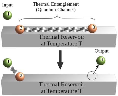
Figure 1: (color online) The teleportation protocol can basically be divided into four steps. Upper panel: The first step is related to the preparation of the entangled resource (qubits 2 and 3) and the input (qubit 1). Here the entangled resource is described by two interacting qubits in thermal equilibrium with a thermal reservoir at temperature $T$. Lower panel: The second step consists in Alice implementing a joint measurement (Bell measurement) in the input and her share of the entangled resource (qubits 1 and 2), which become entangled. Step three is the broadcasting to Bob, via a classical communication channel, of Alice’s measurement result. In the fourth and last step, Bob implements a unitary operation on the output state (qubit 3) depending on the result of Alice’s measurement. Note that the present analysis is particularly relevant and meaningful whenever the overall time needed to implement all steps of the teleportation protocol is lower than the time needed by the whole system to be brought back to thermal equilibrium. In other words, the rate at which we implement all steps of the teleportation protocol must be higher than the system’s thermal relaxation rate. In the opposite scenario, however, Bob’s output qubit would return to a thermal equilibrium state before we could access and further manipulate its content or even before we could finish the teleportation protocol. In this case the present analysis does not apply.

II The mathematical tools

Since the entangled resource in the present manuscript is not a pure state, we have to recast the original teleportation protocol using the language of density matrices. This was done for the deterministic protocol in Ref. for15 and for the probabilistic protocol in Ref. for16 . In Secs. II.1 and II.2 we review the main ideas and results of those references that are needed here. We follow closely the notation and style of Refs. for15 ; for16 . In Sec. II.3 we present the Heisenberg model, preparing the ground for Sec. III, where we show the main results of this manuscript.

II.1 Recasting the teleportation protocol in the density matrix formalism

The input qubit that is teleported from Alice to Bob is assumed a pure state and is given by $|\psi\rangle_{in}=a|0\rangle+b|1\rangle$, with $|a|^{2}+|b|^{2}=1$. Its density matrix is

$$\rho_{in}=|\psi\rangle_{in}\;{}_{in}\langle\psi|=\left(\begin{array}[]{cc}|a|^{2}&ab^{*}\\ a^{*}b&|b|^{2}\end{array}\right),$$ (1)

where $*$ is complex conjugation and the subscript $in$ means “input”. The entangled state shared between Alice and Bob (the quantum communication channel) is described by the canonical ensemble density matrix,

$$\rho_{ch}=\frac{e^{-\frac{H}{kT}}}{Z}=\frac{e^{-\beta H}}{Z},$$ (2)

where $Z=\mbox{Tr}(e^{-H/kT})$ is the partition function, “Tr” is the trace operation, $k$ is the Boltzmann constant, and $ch$ means the quantum communication “channel”. The Hamiltonian $H$ is given by the Heisenberg model as explained in Sec. II.3. Note that the expression “communication channel” refers to any physical apparatus, device or system whereby Alice and Bob may send either classical or quantum information. In the former case we call it a classical communication channel and in the latter a quantum communication channel. Throughout this text the words entangled resource and quantum communication channel are synonyms.

At this stage, the total state describing all qubits is

$$\rho=\rho_{in}\otimes\rho_{ch}.$$ (3)

The teleportation protocol proceeds as follows:

1. Alice implements a Bell state measurement onto qubits 1 and 2.

2. Alice broadcasts her measurement result to Bob using a classical communication channel.

3. Bob uses the information received in step (ii) to choose the right unitary operation to be applied on his state (qubit 3).

If Alice and Bob shared a maximally entangled pure state (Bell state), at the end of step (iii) Bob’s qubit would be exactly described by $\rho_{in}$. In any realistic scenario this is not the case and we invariably have a mixed state describing the quantum communication channel, leading to a non-perfect teleportation.

The projectors describing Alice’s measurement on the input qubit and her qubit of the entangled resource are

$$P_{j}^{\varphi}=|B_{j}^{\varphi}\rangle\langle B_{j}^{\varphi}|,\hskip 14.22636ptj=1,2,3,4,$$ (4)

with

$$|B_{1}^{\varphi}\rangle = \cos\varphi|00\rangle+\sin\varphi|11\rangle,$$ (5)

$$|B_{2}^{\varphi}\rangle = \sin\varphi|00\rangle-\cos\varphi|11\rangle,$$ (6)

$$|B_{3}^{\varphi}\rangle = \cos\varphi|01\rangle+\sin\varphi|10\rangle,$$ (7)

$$|B_{4}^{\varphi}\rangle = \sin\varphi|01\rangle-\cos\varphi|10\rangle.$$ (8)

In the standard protocol $\varphi=\pi/4$ and $|B_{j}\rangle$, $j=1,2,3,4$, are respectively the Bell states $|\Phi^{+}\rangle,|\Phi^{-}\rangle,|\Psi^{+}\rangle$, and $|\Psi^{-}\rangle$ ben93 . Here $\varphi$ is a free parameter chosen by Alice to maximize the efficiency of the probabilistic teleportation.

Alice’s probability to measure a given generalized Bell state is

$$Q_{j}(|\psi\rangle_{in})=\mbox{Tr}[{P_{j}^{\varphi}\rho}]$$ (9)

and at the end of step (iii) Bob’s state is

$$\rho_{{}_{B_{j}}}=\frac{U_{j}\mbox{Tr}_{12}[P_{j}^{\varphi}\rho P_{j}^{\varphi}]U_{j}^{\dagger}}{Q_{j}(|\psi\rangle_{in})}.$$ (10)

Here $\mbox{Tr}_{12}$ is the partial trace on the first two qubits (Alice’s qubits). We make it explicit the dependence of $Q_{j}$ on the input state $|\psi\rangle_{in}$ since for mixed state entangled resources, or non-maximally entangled ones, the probability depends on the input state guo00 ; agr02 ; rig06 ; for15 ; for16 .

In the standard teleportation protocol the unitary transformation that Bob implements on his qubit depends not only on Alice’s measurement outcome but also on the entangled resource ben93 . For example, if $\rho_{ch}$ is the Bell state $|\Phi^{+}\rangle=(|00\rangle+|11\rangle)/\sqrt{2}$ we have $U_{1}=\mathbb{1}$, $U_{2}=\sigma_{z},U_{3}=\sigma_{x}$, and $U_{4}=\sigma_{z}\sigma_{x}$, with $\mathbb{1}$ being the identity matrix and $\sigma_{z}$ and $\sigma_{x}$ the standard Pauli matrices. For the other three Bell states, $|\Phi^{-}\rangle,|\Psi^{+}\rangle$, and $|\Psi^{-}\rangle$, we have respectively $\{U_{1},U_{2},U_{3},U_{4}\}=\{\sigma_{z},\mathbb{1},\sigma_{z}\sigma_{x},\sigma_{x}\},\{\sigma_{x},\sigma_{z}\sigma_{x},\mathbb{1},\sigma_{z}\}$, and $\{\sigma_{z}\sigma_{x},\sigma_{x},\sigma_{z},\mathbb{1}\}$. With that in mind, when we search for the optimal settings leading to the greatest efficiency for the teleportation protocol, we will also let $U_{j}$ run over its possible four values: $\mathbb{1},\sigma_{z},\sigma_{x},\sigma_{z}\sigma_{x}$.

Before we proceed it is worth better explaining what we mean by optimal settings or an optimal protocol. In the following we will be looking for the optimal protocols for several entangled resources shared between Alice and Bob. Our search for the optimal protocols, the ones leading to the greatest efficiencies (average fidelities), will be restricted to projective measurements that Alice might implement on her qubits and Bob will be restricted to act on his qubit using only Pauli matrices, as explained in the previous paragraph. We decided to work only with projective measurements and with unitary operations given by Pauli matrices because those are the resources employed in the original protocol and readily implementable with current technology. It lies beyond the scope and aim of this work to deal with more general types of measurements and more general unitary operations.

II.2 Success rate and efficiency of the probabilistic teleportation

Since the chance $Q_{j}$ of Alice measuring the generalized Bell state $|B_{j}^{\varphi}\rangle$ when she shares with Bob a non-maximally entangled resource depends on the input state $|\psi\rangle_{in}$ guo00 ; agr02 ; rig06 ; for15 ; for16 , we assume $|\psi\rangle_{in}$ is given by a uniform probability distribution,

$$P_{X}(x)=\mathcal{P}(|\psi\rangle_{in}).$$ (11)

Here $X$ denotes a continuous random variable whose values $x$ are all possible pure qubits that together define the sample space $\Omega$. Averaging over this distribution we obtain input-state-independent results for the relevant quantities needed to study the efficiency of the teleportation protocol. The probability distribution $P_{X}(x)$ is normalized as follows,

$$\int_{\Omega}P_{X}(x)dx=\int_{\Omega}\mathcal{P}(|\psi\rangle_{in})d|\psi\rangle_{in}=1,$$ (12)

where $P_{X}(x)$ is constant for all $x$.

If we write an arbitrary qubit as

$$|\psi\rangle=\alpha|0\rangle+\delta e^{i\gamma}|1\rangle,$$ (13)

where $\alpha\geq 0$, $\delta\geq 0$, $\alpha^{2}+\delta^{2}=1$, and $0\leq\gamma\leq 2\pi$ are real numbers, it is not difficult to see that we can select $\alpha^{2}$ and $\gamma$ as independent variables. Thus $\mathcal{P}(|\psi\rangle_{in})=\mathcal{P}(\alpha^{2},\gamma)$ and Eq. (12) reads

$$\int_{0}^{2\pi}\int_{0}^{1}\mathcal{P}(\alpha^{2},\gamma)\mathrm{d}\alpha^{2}\mathrm{d}\gamma=1,$$ (14)

where

$$\mathcal{P}(\alpha^{2},\gamma)=\frac{1}{2\pi}$$ (15)

for a uniform distribution.

It is worth mentioning that the described averaging over pure states does not correspond to a uniform distribution on the Bloch sphere. The distribution as given here states that the relative phase between the states $|0\rangle$ and $|1\rangle$ is completely random as well as the probability weight of the state $|0\rangle$ (or $|1\rangle$) in the superposition of $|0\rangle$ and $|1\rangle$. Nevertheless, this distribution is easy to implement in the laboratory and from a mathematical and operational point of view, we have observed that it simplifies the calculations of the average fidelities, in particular for the probabilistic protocols.

There is also a discrete variable $J$ with values $j=1,2,3,4$ (or $j=\Phi^{+},\Phi^{-},\Psi^{+},\Psi^{-}$) representing the generalized Bell states $|B_{j}^{\varphi}\rangle$. Thus, the probability to measure $|B_{j}^{\varphi}\rangle$ is denoted by $P_{J}(j)$. The conditional probability $P_{J|X}(j|x)$ gives Alice’s chance of measuring the Bell state $j$ if the input state to be teleported is $x$ and is given by Eq. (9),

$$P_{J|X}(j|x)=Q_{j}(|\psi\rangle_{in}).$$ (16)

The joint probability distribution $P_{XJ}(x,j)=P_{JX}(j,x)$ can be obtained if we use the definition of the conditional probability,

$$P_{XJ}(x,j)=P_{X}(x)P_{J|X}(j|x)=\mathcal{P}(|\psi\rangle_{in})Q_{j}(|\psi\rangle_{in}),$$ (17)

which subsequently allows us to compute the marginal distribution $P_{J}(j)=\int_{\Omega}P_{XJ}(x,j)dx$,

$$P_{J}(j)=\int_{\Omega}\mathcal{P}(|\psi\rangle_{in})Q_{j}(|\psi\rangle_{in})d|\psi\rangle_{in}.$$ (18)

And if we use Eq. (17) exchanging the roles of $X$ with $J$ and Eq. (18) we arrive at

$$P_{X|J}(x|j) = \frac{P_{XJ}(x,j)}{P_{J}(j)}$$ (19)

$$= \frac{\mathcal{P}(|\psi\rangle_{in})Q_{j}(|\psi\rangle_{in})}{\int_{\Omega}\mathcal{P}(|\psi\rangle_{in})Q_{j}(|\psi\rangle_{in})d|\psi\rangle_{in}}.$$

These last two expressions, Eqs. (18) and (19), are the probability distributions needed to quantitatively study the probabilistic teleportation protocol.

We can better appreciate the last statement remembering the meaning of $P_{J}(j)$ and $P_{X|J}(x|j)$. Noting that $P_{J}(j)$ gives the chance of Alice measuring the generalized Bell state $|B_{j}^{\varphi}\rangle$ when the distribution for the input states is $\mathcal{P}(|\psi\rangle_{in})$, it is straightforward to see that $P_{J}(j)$ is the average probability of measuring $|B_{j}^{\varphi}\rangle$,

$$\overline{Q}_{j}=P_{J}(j)=\int_{\Omega}\mathcal{P}(|\psi\rangle_{in})Q_{j}(|\psi\rangle_{in})d|\psi\rangle_{in}.$$ (20)

$\overline{Q}_{j}$ does not dependent on $|\psi\rangle_{in}$ and is called the probability of success or the success rate of the probabilistic teleportation protocol if we postselect the measurement result $j$ for16 .

To quantify how similar to the input state is the output after one run of the protocol we employ the fidelity uhl76 , which for a pure input state is

$$F_{j}(|\psi\rangle_{in})=\mbox{Tr}[\rho_{in}\rho_{{}_{B_{j}}}]=\,_{in}\langle\psi|\rho_{{}_{B_{j}}}|\psi\rangle_{in},$$ (21)

with $\rho_{{}_{B_{j}}}$, Eq. (10), being the output state with Bob after the teleportation protocol ends. For a perfect teleportation $F_{j}=1$ (its maximal value) and $F_{j}=0$ (its minimal value) when the output is orthogonal to the input state.

Looking at Eq. (21) we see that in general $F_{j}$ depends on $|\psi\rangle_{in}$ and by averaging over all possible input states we get an input-state-independent quantification for the efficiency of the protocol for16 . Since we are interested in a postselected measurement result $j$, the distribution of input states $|\psi\rangle_{in}$ in this situation is $P_{X|J}(x|j)$, Eq. (19), which leads to the following average fidelity,

$$\overline{F}_{j} = \int_{\Omega}F_{j}(x)P_{X|J}(x|j)dx$$ (22)

$$= \frac{\int_{\Omega}F_{j}(|\psi\rangle_{in})\mathcal{P}(|\psi\rangle_{in})Q_{j}(|\psi\rangle_{in})d|\psi\rangle_{in}}{\int_{\Omega}\mathcal{P}(|\psi\rangle_{in})Q_{j}(|\psi\rangle_{in})d|\psi\rangle_{in}}.$$

This is what we call the efficiency of the probabilistic teleportation protocol if we postselect the measurement result $j$ for16 . If all measurement results are accepted, i.e., no postselection is made, we get back the efficiency of the deterministic protocol for15 ; for16 ,

$$\langle\overline{F}\rangle=\sum_{j=1}^{4}P_{J}(j)\overline{F}_{j}=\int_{\Omega}\overline{F}(|\psi\rangle_{in})\mathcal{P}(|\psi\rangle_{in})d|\psi\rangle_{in},$$ (23)

where $\overline{F}(|\psi\rangle_{in})=\sum_{j}^{4}Q_{j}(|\psi\rangle_{in})F_{j}(|\psi\rangle_{in})$.

Following the strategy of Ref. for16 , we want to maximize Eq. (22) over the set of free parameters present in the probabilistic protocol. In particular, we want to get scenarios in which $\overline{F}_{j}>\langle\overline{F}\rangle$, where $\langle\overline{F}\rangle$ is the optimal efficiency of the deterministic teleportation protocol.

II.3 The Heisenberg model

The Hamiltonian describing the Heisenberg model for a spin-1/2 chain of two qubits is

$$H=j_{x}\sigma_{x}^{(2)}\sigma_{x}^{(3)}+j_{y}\sigma_{y}^{(2)}\sigma_{y}^{(3)}+j_{z}\sigma_{z}^{(2)}\sigma_{z}^{(3)}+h_{a}\sigma_{z}^{(2)}+h_{b}\sigma_{z}^{(3)},$$ (24)

where $\sigma_{j}^{(2)}\sigma_{j}^{(3)}=\sigma_{j}^{(2)}\otimes\sigma_{j}^{(3)}$, with the superscripts $(2)$ and $(3)$ representing qubits 2 (with Alice) and 3 (with Bob) of the quantum communication channel (see Fig. 1). In Eq. (24), $\sigma_{j}$, $j=x,y,z$, are the standard Pauli matrices such that $\sigma_{z}|0\rangle=|0\rangle$ and $\sigma_{z}|1\rangle=-|1\rangle$, $\sigma_{x}|0\rangle=|1\rangle$ and $\sigma_{x}|1\rangle=|0\rangle$, and $\sigma_{y}|0\rangle=i|1\rangle$ and $\sigma_{y}|1\rangle=-i|0\rangle$, with $i$ being the imaginary unity. Furthermore, $j_{x},j_{y},j_{z},h_{a},h_{b}$ are real numbers with the former three representing the coupling constants between the qubits and the latter two denoting external magnetic fields applied respectively on qubits 2 and 3 along the $z$ direction.

Inserting Eq. (24) into Eq. (2) we get the canonical ensemble density matrix describing the quantum communication channel $\rho_{ch}$, which together with Eq. (1) allows us to compute the total state $\rho$ initially describing all three qubits employed in the teleportation protocol (see Eq. (3)). Using $\rho$ we can evaluate Eq. (9) and insert it along with Eq. (15) into Eq. (20) to obtain the four success rates $\overline{Q}_{j}$, each of which is associated with the average probability of measuring the generalized Bell state $|B_{j}^{\varphi}\rangle$. Those success rates can be written as follows,

$$\overline{Q}_{1}=\overline{Q}_{4} = q(\varphi),$$ (25)

$$\overline{Q}_{2}=\overline{Q}_{3} = q(\pi/2\pm\varphi),$$ (26)

where

$$q(\varphi)=\frac{1}{4}-\frac{\cos(2\varphi)\left[\eta\Delta_{h}\sinh(\beta\chi)+\chi\Sigma_{h}e^{2\beta j_{z}}\sinh(\beta\eta)\right]}{4\chi\eta\left[\cosh(\beta\chi)+e^{2\beta j_{z}}\cosh(\beta\eta)\right]}.$$ (27)

In Eq. (27), $\beta=1/kT$ and $\varphi$ were already defined in Eqs. (2) and (4), respectively, while the other quantities are given as follows,

$$\eta=\sqrt{\Delta_{j}^{2}+\Sigma_{h}^{2}}, \Delta_{j}=j_{x}-j_{y}, \Sigma_{h}=h_{a}+h_{b},$$ (28)

$$\chi=\sqrt{\Delta_{h}^{2}+\Sigma_{j}^{2}}, \Delta_{h}=h_{a}-h_{b}, \Sigma_{j}=j_{x}+j_{y}.$$ (29)

We now turn our attention to the efficiency of the teleportation protocol (average fidelities). Before we proceed it is important to recall that the unitary operation $U_{j}$ that Bob must implement on his qubit at the end of the protocol depends, in addition to Alice’s measurement result, on which quantum communication channel (entangled state) she shares with Bob. In the original protocol ben93 , for each one of the four possible Bell states (maximally entangled pure states) that Alice and Bob might share, we can associate a set $S$ containing four $U_{j}$. Each member of $S$ corresponds to the unitary operation that Bob needs to implement on his qubit according to Alice’s measurement result (see Sec. II.1).

Here we deal with a mixed state entangled resource which, similarly to any two-qubit state, can be written as $\rho_{ch}=p_{\!{}_{\Phi^{+}}}|\Phi^{+}\rangle\langle\Phi^{+}|+p_{\!{}_{\Phi^{-}}}|\Phi^{-}\rangle\langle\Phi^{-}|+p_{\!{}_{\Psi^{+}}}|\Psi^{+}\rangle\langle\Psi^{+}|+p_{\!{}_{\Psi^{-}}}|\Psi^{-}\rangle\langle\Psi^{-}|$ $+$ non-diagonal terms. We are employing the Bell states as a basis to expand $\rho_{ch}$ and thus $p_{j}$, $j=\Phi^{+},\Phi^{-},\Psi^{+},\Psi^{-}$, are the probabilities of projecting $\rho_{ch}$ onto the respective Bell states. Depending on the parameters of Eq. (24), one (or more) $p_{j}$ dominates and it is expected that the set $S$ associated with the corresponding Bell state will yield the best efficiency for the teleportation protocol. Therefore, in our search for the optimal protocol, we compute the efficiencies of the probabilistic and deterministic protocols, Eqs. (22) and (23), using the four possible sets $S$. In the end, i.e., after we optimize all expressions with respect to the free parameters of the protocol, we pick out of all possibilities the one giving the greatest efficiency.

II.3.1 The deterministic protocol

Let us begin analyzing the efficiency for the deterministic protocol, Eq. (23), where we append a superscript to $\langle\overline{F}\rangle$ to remind us of which set $S=\{U_{1},U_{2},U_{3},U_{4}\}$ of unitary operations we employ in the calculation of $\langle\overline{F}\rangle$. For example, $\langle\overline{F}\rangle^{\!{}^{\Phi^{+}}}$ means that we use the set $S$ associated to the case where the entangled resource is the Bell state $|\Phi^{+}\rangle$ (see Sec. II.1). Using Eqs. (9), (10), (15), and (21) in Eq. (23) we get

$$\langle\overline{F}\rangle^{\!{}^{\Phi^{+}}} = f^{\!{}_{\Phi}}(\varphi),$$ (30)

$$\langle\overline{F}\rangle^{\!{}^{\Phi^{-}}} = f^{\!{}_{\Phi}}(-\varphi),$$ (31)

$$\langle\overline{F}\rangle^{\!{}^{\Psi^{+}}} = f^{\!{}_{\Psi}}(\varphi),$$ (32)

$$\langle\overline{F}\rangle^{\!{}^{\Psi^{-}}} = f^{\!{}_{\Psi}}(-\varphi),$$ (33)

where

$$f^{\!{}_{\Phi}}(\varphi) = \frac{1}{3}+\frac{\chi\cosh(\beta\chi)-\Sigma_{j}\sin(2\varphi)\sinh(\beta\chi)}{3\chi\left[\cosh(\beta\chi)+e^{2\beta j_{z}}\cosh(\beta\eta)\right]},$$ (34)

$$f^{\!{}_{\Psi}}(\varphi) = \frac{1}{3}+\frac{\eta\cosh(\beta\eta)-\Delta_{j}\sin(2\varphi)\sinh(\beta\eta)}{3\eta\left[e^{-2\beta j_{z}}\cosh(\beta\chi)+\cosh(\beta\eta)\right]}.$$ (35)

Looking at Eqs. (34) and (35), and noting that $\beta$, $\chi$, and $\eta$ are positive quantities, we easily see that the optimal expressions are obtained by setting $\varphi=\pm\pi/4$. In other words, the measurement basis Alice must employ is the standard Bell basis. More specifically, we must choose $\varphi$ such that $-\Sigma_{j}\sin(2\varphi)=|\Sigma_{j}|$ and $-\Delta_{j}\sin(2\varphi)=|\Delta_{j}|$. If $\Sigma_{j}<0$ we choose $\varphi=\pi/4$ and when $\Sigma_{j}>0$ we set $\varphi=-\pi/4$ (or $5\pi/4$). A similar analysis applies to $\Delta_{j}$. Therefore, the optimal average fidelities for each set $S$ are

$$\langle\overline{F}\rangle^{\!{}^{\Phi^{+}}}_{\!{}_{opt}}= \langle\overline{F}\rangle^{\!{}^{\Phi^{-}}}_{\!{}_{opt}} =f^{\!{}_{\Phi}}_{\!{}_{opt}},$$ (36)

$$\langle\overline{F}\rangle^{\!{}^{\Psi^{+}}}_{\!{}_{opt}}= \langle\overline{F}\rangle^{\!{}^{\Psi^{-}}}_{\!{}_{opt}} =f^{\!{}_{\Psi}}_{\!{}_{opt}},$$ (37)

where

$$f^{\!{}_{\Phi}}_{\!{}_{opt}} = \frac{1}{3}+\frac{\chi\cosh(\beta\chi)+|\Sigma_{j}|\sinh(\beta\chi)}{3\chi\left[\cosh(\beta\chi)+e^{2\beta j_{z}}\cosh(\beta\eta)\right]},$$ (38)

$$f^{\!{}_{\Psi}}_{\!{}_{opt}} = \frac{1}{3}+\frac{\eta\cosh(\beta\eta)+|\Delta_{j}|\sinh(\beta\eta)}{3\eta\left[e^{-2\beta j_{z}}\cosh(\beta\chi)+\cosh(\beta\eta)\right]}.$$ (39)

Finally, the optimal efficiency for the deterministic teleportation protocol is given by

$$\langle\overline{F}\rangle_{\!{}_{opt}}=\max\{f^{\!{}_{\Phi}}_{\!{}_{opt}},f^{\!{}_{\Psi}}_{\!{}_{opt}}\}.$$ (40)

Equation (40) is the benchmark we want to surpass using the probabilistic protocol.

II.3.2 The probabilistic protocol

Following the superscript notation just introduced in the preceding analysis, we now need to evaluate $\overline{F}_{j}^{\;\epsilon}$, Eq. (22), for $j=1,2,3,4$ and $\epsilon=\Phi^{+},\Phi^{-},\Psi^{+},\Psi^{-}$. Here each $j$ represents one of the four possible measurement outcomes of Alice, i.e., it denotes which generalized Bell state $|B^{\varphi}_{j}\rangle$ she measured, and $\epsilon$ represents which set of unitary operations $S$ Bob uses to properly correct his qubit, where each element of the set corresponds to a given measurement result of Alice. For instance, $\overline{F}_{1}^{\,{}_{\Phi^{+}}}$ means that Alice and Bob are working with the postselected measurement outcome $|B^{\varphi}_{1}\rangle$, discarding the other three possible measurement results, and Bob’s unitary operation for all valid runs of the protocol is always $\mathbb{1}$ (the respective $U_{1}$ associated with $\epsilon=\Phi^{+}$). In Table 1 we list all $16$ possibilities.

Table 1: In the table below we list to each $\overline{F}_{j}^{\,{}_{\epsilon}}$ the corresponding Alice’s measurement outcome $|B_{j}^{\varphi}\rangle$ and the respective unitary operation Bob implements on his qubit.

$\overline{F}_{1}^{\,{}_{\Phi^{+}}}\longrightarrow$ $|B^{\varphi}_{1}\rangle\longrightarrow$ $\mathbb{1}$ $\overline{F}_{2}^{\,{}_{\Phi^{+}}}\longrightarrow$ $|B^{\varphi}_{2}\rangle\longrightarrow$ $\sigma_{z}$ $\overline{F}_{3}^{\,{}_{\Phi^{+}}}\longrightarrow$ $|B^{\varphi}_{3}\rangle\longrightarrow$ $\sigma_{x}$ $\overline{F}_{4}^{\,{}_{\Phi^{+}}}\longrightarrow$ $|B^{\varphi}_{4}\rangle\longrightarrow$ $\sigma_{z}\sigma_{x}$

$\overline{F}_{1}^{\,{}_{\Phi^{-}}}\longrightarrow$ $|B^{\varphi}_{1}\rangle\longrightarrow$ $\sigma_{z}$ $\overline{F}_{2}^{\,{}_{\Phi^{-}}}\longrightarrow$ $|B^{\varphi}_{2}\rangle\longrightarrow$ $\mathbb{1}$ $\overline{F}_{3}^{\,{}_{\Phi^{-}}}\longrightarrow$ $|B^{\varphi}_{3}\rangle\longrightarrow$ $\sigma_{z}\sigma_{x}$ $\overline{F}_{4}^{\,{}_{\Phi^{-}}}\longrightarrow$ $|B^{\varphi}_{4}\rangle\longrightarrow$ $\sigma_{x}$

$\overline{F}_{1}^{\,{}_{\Psi^{+}}}\longrightarrow$ $|B^{\varphi}_{1}\rangle\longrightarrow$ $\sigma_{x}$ $\overline{F}_{2}^{\,{}_{\Psi^{+}}}\longrightarrow$ $|B^{\varphi}_{2}\rangle\longrightarrow$ $\sigma_{z}\sigma_{x}$ $\overline{F}_{3}^{\,{}_{\Psi^{+}}}\longrightarrow$ $|B^{\varphi}_{3}\rangle\longrightarrow$ $\mathbb{1}$ $\overline{F}_{4}^{\,{}_{\Psi^{+}}}\longrightarrow$ $|B^{\varphi}_{4}\rangle\longrightarrow$ $\sigma_{z}$

$\overline{F}_{1}^{\,{}_{\Psi^{-}}}\longrightarrow$ $|B^{\varphi}_{1}\rangle\longrightarrow$ $\sigma_{z}\sigma_{x}$ $\overline{F}_{2}^{\,{}_{\Psi^{-}}}\longrightarrow$ $|B^{\varphi}_{2}\rangle\longrightarrow$ $\sigma_{x}$ $\overline{F}_{3}^{\,{}_{\Psi^{-}}}\longrightarrow$ $|B^{\varphi}_{3}\rangle\longrightarrow$ $\sigma_{z}$ $\overline{F}_{4}^{\,{}_{\Psi^{-}}}\longrightarrow$ $|B^{\varphi}_{4}\rangle\longrightarrow$ $\mathbb{1}$

Inserting Eqs. (9), (15), and (21) into (22), and using the proper unitary operation $U_{j}$ (see Table 1) to compute $\rho_{\!{}_{B_{j}}}$, Eq. (10), we get

$$\overline{F}_{1}^{\,{}_{\Phi^{+}}}=\overline{F}_{4}^{\,{}_{\Phi^{+}}} = g^{\,{}_{\Phi}}(\varphi),$$ (41)

$$\overline{F}_{2}^{\,{}_{\Phi^{+}}}=\overline{F}_{3}^{\,{}_{\Phi^{+}}} = g^{\,{}_{\Phi}}(\pi/2-\varphi),$$ (42)

$$\overline{F}_{1}^{\,{}_{\Phi^{-}}}=\overline{F}_{4}^{\,{}_{\Phi^{-}}} = g^{\,{}_{\Phi}}(-\varphi),$$ (43)

$$\overline{F}_{2}^{\,{}_{\Phi^{-}}}=\overline{F}_{3}^{\,{}_{\Phi^{-}}} = g^{\,{}_{\Phi}}(\pi/2+\varphi),$$ (44)

$$\overline{F}_{1}^{\,{}_{\Psi^{+}}}=\overline{F}_{4}^{\,{}_{\Psi^{+}}} = g^{\,{}_{\Psi}}(\varphi),$$ (45)

$$\overline{F}_{2}^{\,{}_{\Psi^{+}}}=\overline{F}_{3}^{\,{}_{\Psi^{+}}} = g^{\,{}_{\Psi}}(\pi/2-\varphi),$$ (46)

$$\overline{F}_{1}^{\,{}_{\Psi^{-}}}=\overline{F}_{4}^{\,{}_{\Psi^{-}}} = g^{\,{}_{\Psi}}(-\varphi),$$ (47)

$$\overline{F}_{2}^{\,{}_{\Psi^{-}}}=\overline{F}_{3}^{\,{}_{\Psi^{-}}} = g^{\,{}_{\Psi}}(\pi/2+\varphi),$$ (48)

where

$$g^{\,{}_{\Phi}}(\varphi) = \frac{1}{3}+\frac{\eta\{\chi\cosh(\beta\chi)-\sinh(\beta\chi)[\Delta_{h}\cos(2\varphi)+\Sigma_{j}\sin(2\varphi)]\}}{3\left\{\eta\chi\left[\cosh(\beta\chi)+e^{2\beta j_{z}}\cosh(\beta\eta)\right]-\cos(2\varphi)\left[\eta\Delta_{h}\sinh(\beta\chi)+\chi\Sigma_{h}e^{2\beta j_{z}}\sinh(\beta\eta)\right]\right\}},$$ (49)

$$g^{\,{}_{\Psi}}(\varphi) = \frac{1}{3}+\frac{\chi\{\eta\cosh(\beta\eta)-\sinh(\beta\eta)[\Delta_{j}\sin(2\varphi)+\Sigma_{h}\cos(2\varphi)]\}}{3\{\eta\chi\left[e^{-2\beta j_{z}}\cosh(\beta\chi)+\cosh(\beta\eta)\right]-\cos(2\varphi)\left[\eta\Delta_{h}e^{-2\beta j_{z}}\sinh(\beta\chi)+\chi\Sigma_{h}\sinh(\beta\eta)\right]\}}.$$ (50)

The first important thing worth noting if we look at Eqs. (49) and (50) is the fact that $\varphi=\pm\pi/4$ (or $\varphi=\pm 3\pi/4$) are not in general the optimal settings. In other words, the optimal measurement basis are not formed by the standard maximally entangled Bell states. Indeed, whenever an external magnetic field is present, either $\Delta_{h}$ or $\Sigma_{h}$ (or both) is not zero. This leads to the presence of the $\cos(2\varphi)$ terms, in addition to the $\sin(2\varphi)$ terms, in Eqs. (49) and (50). The optimal $\varphi$ in this case can be found by solving the equations $dg^{\epsilon}/d\varphi=0$, $\epsilon=\Phi,\Psi$, and then selecting the $g^{\epsilon}$ giving the greatest efficiency.

Second, comparing Eqs. (49) and (50) with (34) and (35), it is not difficult to see that

$$g^{\epsilon}(\varphi)=f^{\epsilon}(\varphi), \Delta_{h}=\Sigma_{h}=0.$$ if (51)

This means that if we have no external fields ($\Delta_{h}=\Sigma_{h}=0$), the probabilistic teleportation protocol gives exactly the same efficiencies of the deterministic protocol. We thus arrive at the important conclusion that the probabilistic protocol can only beat the deterministic one if external magnetic fields are turned on.

There is another interesting feature of the present probabilistic protocol. Looking at Eqs. (41)-(48) we see that we always have $\overline{F}_{1}^{{\epsilon}}=\overline{F}_{4}^{{\epsilon}}$ and $\overline{F}_{2}^{{\epsilon}}=\overline{F}_{3}^{{\epsilon}}$, which implies that $\overline{F}_{1}^{{\epsilon}}$ and $\overline{F}_{4}^{{\epsilon}}$, and equivalently $\overline{F}_{2}^{{\epsilon}}$ and $\overline{F}_{3}^{{\epsilon}}$, share the same optimal $\varphi$. This property enhances the effective success rate of the probabilistic protocol since two out of four possible measurement results of Alice give the same optimal efficiency with the same optimal settings. Thus, instead of postselecting only one outcome, Alice and Bob can postselect two measurement outcomes, increasing the success rate to twice the value given in Eq. (27),

$$\overline{Q}_{1,4} = 2q(\varphi),$$ (52)

$$\overline{Q}_{2,3} = 2q(\varphi\pm\pi/2).$$ (53)

Finally, putting together all the pieces of information in the last paragraphs, and noting that in Eqs. (49) and (50) the arguments of all sines and cosines are given by $2\varphi$, we can obtain the optimal efficiency for the probabilistic protocol by solving the following maximization problem,

$$\overline{F}_{\!{}_{opt}}=\max_{\varphi\in[0,\pi]}\{g^{\!{}_{\Phi}}(\varphi),g^{\!{}_{\Psi}}(\varphi)\}.$$ (54)

By ranging $\varphi$ from $0$ to $\pi$ we can obtain the optimal settings for all instances listed in Eqs. (41)-(48), and by choosing the greatest value from $g^{\!{}_{\Phi}}(\varphi_{opt})$ and $g^{\!{}_{\Psi}}(\tilde{\varphi}_{opt})$, we get the optimal efficiency $\overline{F}_{\!{}_{opt}}$. The corresponding success rate is given by either $2q(\varphi_{opt})$ or $2q(\tilde{\varphi}_{opt})$, where $\varphi_{opt}$ and $\tilde{\varphi}_{opt}$ are the $\varphi$’s maximizing $g^{\!{}_{\Phi}}$ and $g^{\!{}_{\Psi}}$, respectively.

III Results

We are now ready to study the efficiency to teleport an arbitrary pure state qubit for several entangled resources described by Heisenberg-like models in thermal equilibrium with a heat reservoir at temperature $T$. We divide our entangled resources into two main groups, all of which subjected to external magnetic fields in the $z$ direction. The first group encompasses all models in which there is no $\sigma_{z}^{(2)}\sigma_{z}^{(3)}$ interaction and the second one those models possessing it. Note that whenever there is no external fields, the deterministic and probabilistic protocols yield the same results and, thus, we work only with cases in which the external field is present.

III.1 XY-like models

The one-dimensional XY model in a transverse field is obtained from Eq. (24) by setting $j_{z}=0$ and $h_{a}=h_{b}$. It is more usual, however, to rewrite Eq. (24) as follows werIJMPB ,

$$H=-\lambda[(1+\zeta)\sigma_{x}^{(2)}\sigma_{x}^{(3)}+(1-\zeta)\sigma_{y}^{(2)}\sigma_{y}^{(3)}]-\sigma_{z}^{(2)}-\sigma_{z}^{(3)},$$ (55)

with $\lambda\geq 0$ being the inverse of the magnitude of the external field and $\zeta$ the anisotropy parameter. The Ising model is obtained when $\zeta=\pm 1$ and for $\zeta=0$ we get the XX model in a transverse field. At $T=0$ and in the thermodynamic limit (infinite chain), the XY model has a quantum critical point at $\lambda=1$, where a second-order quantum phase transition separates a ferromagnetic ordered phase from a paramagnetic one lie61 ; bar70 ; bar71 ; pfe70 .

III.1.1 Efficiency as a function of $T$

We first analyze the optimal efficiencies (average fidelities) of the deterministic and probabilistic protocols, Eqs. (40) and (54) respectively, as a function of the temperature $T$. We start with the Ising model in a transverse field, whose main results are shown in Fig. 2.

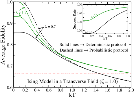
Figure 2: (color online) Main plot: The efficiencies for the deterministic (solid curves) and probabilistic (dashed curves) teleportation protocols as a function of the temperature when the quantum communication channel connecting Alice and Bob is given by the thermalized Ising model in a transverse field. The efficiency for the deterministic protocol is given by Eq. (40) and for the probabilistic one by Eq. (54). The dotted-dashed red line marks the classical limit ($2/3$) below which the teleportation protocol can be matched by a purely classical protocol. Inset: The success rate (probability of success) for the probabilistic protocol. Here and in the following figures all quantities are dimensionless.

Looking at Fig. 2 we note that the efficiency is a monotonically decreasing function of the temperature and that for $kT\approx 1.2$ the optimal efficiencies for the deterministic and probabilistic protocols are almost the same. As we continue to increase the temperature, we arrive at a value of $T$ after which the efficiency of the protocol is below $2/3$. This value for the average fidelity is called the classical limit since any protocol with average fidelities lower than $2/3$ can be implemented without Alice and Bob sharing an entangled resource mas95 . See also the Appendix for further details and a proof of this limit for the deterministic teleportation protocol studied here.

For low values of $T$, however, we can have considerable gains in efficiency by working with the probabilistic protocol. For instance, whenever $kT<0.2$, the probabilistic protocol yields an almost perfect teleportation, a considerable improvement over the deterministic one. In this case the success rate is about $10\%$ when $\lambda=0.7$ and $30\%$ when $\lambda=1.3$. We also note that the optimal efficiencies for the deterministic and probabilistic protocols are given by $f^{\!{}_{\Phi}}_{opt}$ and $g^{\!{}_{\Phi}}(\varphi)$, respectively (see Eqs. (40) and (54)). Moreover, the optimal $\varphi$ for the latter depends on $T$ and is not equal to $\pm\pi/4$.

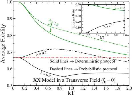
Figure 3: (color online) Same as Fig. 2 but now we work with the isotropic XX model in a transverse field. Note that under certain conditions ($\lambda<1$) the efficiency for the probabilistic protocol may increase with the temperature and be the only one yielding an efficiency greater than the classical threshold (2/3). Also, the optimal $\varphi$ for the probabilistic protocol depends on $T$ and is not equal to $\pm\pi/4$, with the latter being the optimal settings for the deterministic case.

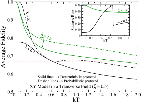
Figure 4: (color online) Same as Figs. 2 and 3 but now we have the anisotropic XY model in a transverse field.

Moving to the XX and XY models, i.e., turning on the $\sigma_{y}^{(2)}\sigma_{y}^{(3)}$ interaction, we observe the following two similar and interesting trends (see Figs. 3 and 4). First, whenever $\lambda<1$ (ferromagnetic phase) there exists a range of values of temperature where the efficiency of the probabilistic protocol increases with $T$. This is a remarkable property and tells us that working with a “warmer” entangled resource is better than working with a “colder” one. We can understand this behavior noting that under certain configurations of the coupling constants, the ground state of the Hamiltonian has little or no entanglement at all, although the first excited states are highly entangled ones and very close to Bell states Rig03 . Thus, by increasing the temperature we start to populate those highly entangled states in such a manner that a warmer entangled resource has more entanglement than a colder one. The latter effect is more intense in the probabilistic protocol where, by postselecting the appropriate measurement results, we may project the entangled resource $\rho_{ch}$ onto highly entangled states and consequently enhance even more the efficiency of the teleportation protocol. If we continue to increase the temperature, however, more and more states get populated and we start to get a less entangled quantum communication channel, reducing the efficiency of the protocol. For sufficiently high temperatures the entangled resource is nearly described by a completely mixed state with no entanglement at all. This is why we always end up with efficiencies lower than $2/3$ for very high temperatures.

Second, another important characteristic shared by the XX and XY models is the fact that for certain values of $T$ the efficiency for the deterministic protocol does not surpass the classical limit $2/3$, while the probabilistic protocol’s efficiency does. In this scenario, therefore, we can only get a truly quantum teleportation if we employ the probabilistic protocol.

There are also different characteristics between the XX and XY models. For example, the deterministic protocol for the XX model does not yield an average fidelity greater than the classical limit for $\lambda<1$. This is only possible when we use the probabilistic protocol. For the XY model, however, there is no such restriction and we can have for $\lambda<1$ the average fidelity for both the deterministic and probabilistic protocols greater than $2/3$ if we work at a sufficiently low temperature.

Another distinctive feature of the XX model is the fact that whenever the optimal average fidelities for the deterministic and probabilistic protocols are greater than $2/3$, $f^{\!{}_{\Psi}}_{opt}$ and $g^{\!{}_{\Psi}}(\varphi)$, respectively, are the functions optimizing the efficiency (see Eqs. (40) and (54)). For the XY model, however, the functions leading to the optimal efficiency for certain values of $T$ may be different for the probabilistic protocol when the efficiency is greater than $2/3$. In this case either $g^{\!{}_{\Phi}}(\varphi)$ or $g^{\!{}_{\Psi}}(\varphi)$ may give the optimal efficiency. This is the reason for the cusp of the curve of the optimal average fidelity (the $\lambda=0.7$ dashed curve) and for the discontinuity in the success rate (the $\lambda=0.7$ curve in the inset) that we see for the probabilistic protocol in Fig. 4. The cusp for the efficiency curve and the discontinuity for the probability of success curve occur exactly at the temperature in which $g^{\!{}_{\Phi}}(\varphi)$ and $g^{\!{}_{\Psi}}(\varphi)$ exchange roles. Below this temperature $g^{\!{}_{\Phi}}(\varphi)$ gives the optimal efficiency while above it $g^{\!{}_{\Psi}}(\varphi)$ does.

III.1.2 Efficiency as a function of the external field

We now turn our attention to the behavior of the average fidelities for the deterministic and probabilistic protocols as functions of the inverse of the strength of the external magnetic field $\lambda$. Starting with the Ising model in a transverse field (upper panel of Fig. 5), we note that for a fixed temperature there is an optimal $\lambda$ that gives the greatest efficiency and that the optimal $\lambda$’s are different for the deterministic and probabilistic protocols. This is most clearly seen looking at the curves for $kT=0.3$. We also see that the probabilistic protocol outperforms by far the deterministic one for small values of $\lambda$.

Studying the XX model (left lower panel of Fig. 5), we note that the greater the value of $\lambda$ the better the efficiency of the probabilistic protocol. For the deterministic protocol, an increase of $\lambda$ increases the efficiency only for $\lambda$ greater than a certain critical value that depends on $T$. Also, when $\lambda<1$ the average fidelity for the deterministic protocol does not exceed $2/3$. It is interesting to note that the efficiencies for the probabilistic protocols, and in particular for the deterministic ones, change abruptly near the quantum critical point $\lambda=1$.

Near the quantum critical point $\lambda=1$ there is a similar abrupt behavior for the efficiencies of the deterministic and probabilistic protocols for the XY model (right lower panel of Fig. 5). In this case the average fidelities tend to their minimum values near the critical point. As we move to the right or left of the critical point the efficiency starts to increase. For $\lambda>1$ this trend continues as we increase $\lambda$ while for $\lambda<1$ the average fidelity starts to decrease after reaching a local maximum. This behavior is clearer the greater the value of $T$. Finally, the reason for the cusps in the curves for the efficiencies is again related to which of the functions $f^{\!{}_{\Phi}}_{opt}$ or $f^{\!{}_{\Psi}}_{opt}$ ($g^{\!{}_{\Phi}}(\varphi)$ or $g^{\!{}_{\Psi}}(\varphi)$) gives the optimal average fidelity for the deterministic (probabilistic) protocol. For small $\lambda$, $f^{\!{}_{\Phi}}_{opt}$ and $g^{\!{}_{\Phi}}(\varphi)$ give the highest efficiencies and, as we increase $\lambda$, $f^{\!{}_{\Psi}}_{opt}$ and $g^{\!{}_{\Psi}}(\varphi)$ dominate after we cross a certain value of $\lambda$ that depends on $T$.

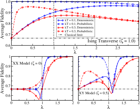
Figure 5: (color online) The optimal efficiencies of the deterministic (solid curves) and probabilistic (dashed curves) teleportation protocols as a function of $\lambda$ for the Ising model (upper panel), the XX model (left lower panel), and the XY model (right lower panel), all of them in an external magnetic field of strength $1/\lambda$. Circles denote $kT=0.1$ and squares $kT=0.3$. The dotted-dashed black lines delimit the classical limit $2/3$.

III.2 XXZ-like models

The one-dimensional XXZ model in an external field in the $z$ direction is obtained from Eq. (24) when we set $j_{x}=j_{y}$ and $h_{a}=h_{b}$. This model is usually written as werIJMPB

$$H=2J[\sigma_{x}^{(2)}\sigma_{x}^{(3)}+\sigma_{y}^{(2)}\sigma_{y}^{(3)}+\Delta\sigma_{z}^{(2)}\sigma_{z}^{(3)}]-\frac{h}{2}[\sigma_{z}^{(2)}+\sigma_{z}^{(3)}],$$ (56)

where $J$ is the exchange constant, $\Delta$ the anisotropy parameter, and $h$ the external field. When $\Delta=1$ we have the isotropic XXX model and for $\Delta\neq 0$ we get the anisotropic XXZ model. In the thermodynamic limit and at $T=0$ the XXZ model has two quantum critical points clo66 ; tak99 ; bor05 ; boo08 ; tri10 : $\Delta_{inf}$, where an infinite order quantum phase transition takes place, and $\Delta_{1}$, where a first-order quantum phase transition happens. The expressions giving those critical points are not so simple and can be found in Refs. clo66 ; tak99 .

III.2.1 Efficiency as a function of $T$

Let us start studying the isotropic XXX model ($\Delta=1$). The first thing worth noting is that for $J<0$ the efficiencies for both the deterministic and probabilistic protocols do not surpass the classical limit $2/3$, even for low $T$. We thus restrict the following analysis to the cases in which $J>0$. It can also be proved that for the deterministic protocol $f^{\!{}_{\Phi}}_{opt}\leq 2/3$ and thus, since we are interested in the cases surpassing the classical limit, instead of Eq. (40) we work only with $f^{\!{}_{\Psi}}_{opt}$ in the determination of the optimal efficiency. The curves for the deterministic protocol in Figs. 6 and 8 show $f^{\!{}_{\Psi}}_{opt}$. Also, by setting the magnetic field to $h=8.0$ we get that the first-order quantum phase transition for this model occurs at $J_{c}=1.0$.

Looking at Fig. 6 we note that we have two regimes for the behavior of the average fidelities. For $J<J_{c}$ the deterministic protocol does not give an efficiency greater than $2/3$. In this regime the classical limit can only be surpassed using the probabilistic protocol. Indeed, for $kT\lesssim 5.0$ the probabilistic protocol yields an efficiency greater than $2/3$ and greater than that of the deterministic protocol, with success rates of the order of $10\%$. We also see that in this range of temperatures there are instances where the efficiency increases with $T$.

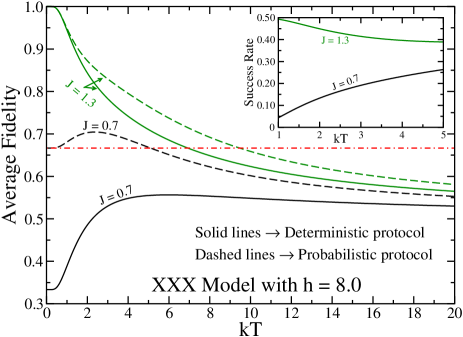
Figure 6: (color online) Main plot: The average fidelities (efficiencies) of the deterministic (solid curves) and probabilistic (dashed curves) teleportation protocols as a function of the temperature when the quantum communication channel connecting Alice and Bob is the thermalized XXX model in an external field. As explained in the text, for the deterministic protocol we plot $f^{\!{}_{\Psi}}_{opt}$ and for the probabilistic one Eq. (54). The dotted-dashed red line marks the classical limit ($2/3$) below which the teleportation protocol can be matched by a purely classical protocol. Inset: The success rate (probability of success) for the probabilistic protocol.

For $J>J_{c}$, on the other hand, both the deterministic and probabilistic protocols can yield efficiencies above the classical limit. In this regime the efficiencies are always a monotonically decreasing function of the temperature and we still have a small range of temperatures in which only the probabilistic protocol gives an average fidelity greater than $2/3$. For all values of $J>0$ the optimal efficiency for the probabilistic protocol is given by $g^{\!{}_{\Psi}}(\varphi)$, with the optimal $\varphi$ being different from $\pm\pi/4$ and dependent on $T$.

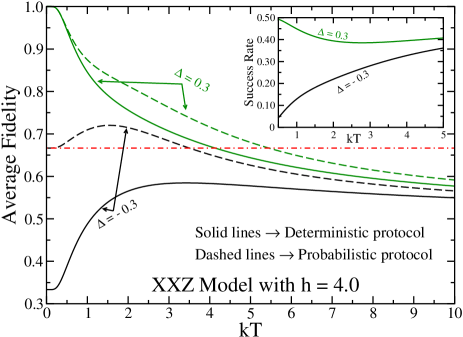
Figure 7: (color online) Same as Fig. 6 but now we work with the XXZ model with an external field in the $z$ direction.

We now focus our attention at the XXZ model in an external field in the $z$ direction. We set $J=1.0$ and the magnitude of the field ($h=4.0$) such that the first-order quantum phase transition occurs at $\Delta_{1}=0$. Here we can also prove that $f^{\!{}_{\Phi}}_{opt}\leq 2/3$ for the deterministic protocol and similarly to the XXX model, we show $f^{\!{}_{\Psi}}_{opt}$ instead of Eq. (40) in Figs. 7 and 8 when analyzing the deterministic protocol.

Looking at Fig. 7 we note that many features seen for the XXX model are also present in the XXZ model. Indeed, we have two regimes for the behavior of the efficiency of the protocol. One before ($\Delta<\Delta_{1}$) and another after ($\Delta>\Delta_{1}$) the quantum critical point delimiting the first-order quantum phase transition. For $\Delta<\Delta_{1}$ only the probabilistic protocol yields average fidelities greater than the classical limit, with success rates lying between $10\%$ to $20\%$ for a considerable set of values of $\Delta<\Delta_{1}$. We also have ranges of temperatures where the efficiency of the probabilistic protocol increases with $T$.

For $\Delta>\Delta_{1}$ the efficiencies are monotonically decreasing functions of $T$ and both the deterministic and probabilistic protocols can work above the classical limit at sufficiently low temperatures. We also have small ranges of $T$ in which the probabilistic protocol leads to an efficiency greater than $2/3$ while the deterministic protocol works below this value.

Finally, and similarly to the XXX model, whenever the efficiency is above the classical limit, the functions leading to the optimal efficiencies are $f^{\!{}_{\Psi}}_{opt}$ for the deterministic and $g^{\!{}_{\Psi}}(\varphi)$ for the probabilistic protocols. The optimal values of $\varphi$ for the probabilistic protocol depend on $T$ and are not $\pm\pi/4$, the optimal ones for the deterministic case.

III.2.2 Efficiency as a function of the coupling constants

We now investigate how the efficiencies (average fidelities) for the deterministic and probabilistic protocols behave as a function of the exchange constant $J$ for the XXX model and of the anisotropy parameter $\Delta$ for the XXZ model.

For the XXX model we keep as before $h=8.0$ and for several values of $kT$ we compute the efficiency as a function of $J$ (upper panel of Fig. 8), including values of $J$ near and at the critical point $J_{c}=1.0$. For the XXZ model we set $h=4.0$ and $J=1.0$, which leads to a critical point $\Delta_{1}=0$, and we also evaluate for several values of $kT$ the efficiency as a function of $\Delta$ (lower panel of Fig. 8), including values of $\Delta$ near and at the critical point $\Delta_{1}$.

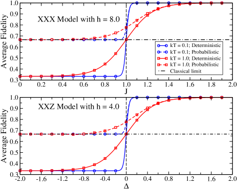
Figure 8: (color online) The optimal efficiencies of the deterministic (solid curves) and probabilistic (dashed curves) teleportation protocols as a function of $J$ for the XXX model (upper panel) and of $\Delta$ for the XXZ model (lower panel). As discussed in the text, for the deterministic protocol we plot $f^{\!{}_{\Psi}}_{opt}$ and for the probabilistic one Eq. (54). Circles denote $kT=0.1$ and squares $kT=1.0$. The dotted-dashed black lines delimit the classical limit $2/3$.

Looking at Fig. 8 we note that the efficiencies for the XXX and XXZ models, as functions of $J$ and $\Delta$, respectively, share the same qualitative features. In particular, we note a clear distinctive behavior for the optimal average fidelities before and after the first-order quantum critical points, even at considerably high temperatures ($kT\approx 1.0$). It is now clear that below the critical point the deterministic protocols do not yield an efficiency greater than the classical limit $2/3$ while the probabilistic protocols do. We also observe that for sufficiently high values of $J$ and $\Delta$, above the critical points, the efficiencies for the deterministic and probabilistic protocols converge to their greatest possible value, leading to a perfect teleportation. Moreover, at low values of $J$ or $\Delta$, the functions $f^{\!{}_{\Phi}}_{opt}$ and $g^{\!{}_{\Phi}}(\varphi)$ give the optimal average fidelities. As we approach the critical point, $f^{\!{}_{\Psi}}_{opt}$ and $g^{\!{}_{\Psi}}(\varphi)$ dominate and furnish the optimal values for the efficiencies. Note that this exchange of functions leading to the optimal efficiencies never occurs exactly at the critical point for finite $T$.

It is also worth noting that we have computed the efficiencies about and at the other quantum critical point, where an infinite-order quantum phase transition happens ($\Delta_{inf}$). For the present XXZ model with $h=4.0$ and $J=1.0$ we obtain $\Delta_{inf}\approx 2.74$ clo66 ; tak99 ; werPRA . We have not observed, however, any quantitative or qualitative changes in the behavior of the efficiencies. Actually, before reaching $\Delta_{inf}$ the efficiency of the teleportation protocol already saturates to its highest possible value and no changes are seen after that value is attained.

IV Conclusion

We have extensively studied the probabilistic teleportation protocol when the entangled resource connecting Alice and Bob is given by interacting two-qubit systems in equilibrium with a thermal reservoir. In this scenario the quantum state describing the entangled resource is the canonical ensemble density matrix and any entanglement present in that state is usually dubbed thermal entanglement Ved01 ; Kam02 ; Rig03 ; Ami07 ; reviews ; Wer10 ; werPRL ; werPRA ; werIJMPB .

We worked with several standard Heisenberg-like models in order to describe the interaction between the two qubits of the quantum communication channel. Those models are widely employed to describe the interaction between two or more spins in several condensed matter systems and can be used to describe the interactions we might face when building a quantum computer or a quantum communication protocol operating on solid state devices. Being more specific, we studied the Ising model, the XX model, the XY model, the isotropic XXX model, and the anisotropic XXZ model. We also considered the cases where an external magnetic field is applied in the $z$ direction.

After studying all those models three important common features emerged. First, we proved analytically that the efficiency for the probabilistic protocol can only be greater than the efficiency of the deterministic protocol if we have an external magnetic field. Whenever the external field is zero, the probabilistic and deterministic protocols have exactly the same efficiency.

Second, whenever the probabilistic teleportation protocol outperforms the deterministic protocol, the measurement basis employed by Alice during the execution of the teleportation protocol is not the standard Bell basis, which is spanned by four maximally entangled states. The optimal measurement basis for the probabilistic protocol is given by the generalized Bell states, whose entanglement degree is not maximal. Moreover, the appropriate generalized Bell basis depends on the value of the temperature and on which Heisenberg-like model we are working with.

Third, the optimal settings leading to the optimal efficiency for the probabilistic protocol are the same for two out of four possible measurement results that Alice may obtain at each run of the protocol. Thus, the success rate for the probabilistic protocol is enhanced since Alice and Bob can postselect two instead of one measurement result at each run of the protocol. In general, the success rate for the probabilistic protocols here studied are above $10\%$, being much higher than this value under certain arrangements.

Other three features are clearly shared by all models here investigated with the exception of the Ising model. The first one is related to the fact that more heat (higher temperatures) may lead to a more efficient probabilistic teleportation. In the notation of the present paper, this happens whenever the coupling constants and the external magnetic field are such that the system lies below the quantum critical point separating its two phases. In the appropriate phase, there exists a scenario in which the efficiency increases with increasing temperature.

Another characteristic shared by almost all models is the fact that under the same conditions the optimal efficiencies for the probabilistic and deterministic protocols may differ in a very important way. There are ranges of temperatures where only the probabilistic protocol crosses the classical limit of $2/3$ for the optimal average fidelity. Below this value any teleportation protocol can be simulated by a “classical” protocol, where no entanglement at all is needed between Alice and Bob. Only local operations and classical communication (LOCC) suffice to deliver the same efficiency. Thus, whenever this happens, we can only have a truly quantum teleportation if we work with the probabilistic protocol. The deterministic protocol fails in delivering a quantum teleportation that is genuinely quantum.

Third, we have also noted that the behavior for the efficiencies of the deterministic and probabilistic protocols may be qualitatively and quantitatively affected in the vicinity of the quantum critical points, even at finite temperatures. For instance, for the XX, XXX and XXZ models the optimal efficiencies can only surpass the classical limit $2/3$ as we approach the critical point from below. The lower the temperature the more the quantum critical point marks this transition in the behavior for the efficiency. For the XX and XY models, we also noted that near the critical point we have the global minimum for the efficiency.

Finally, and similarly to the results of Ref. for16 , we have a trade-off between the success rates and the efficiencies for the probabilistic protocols. The optimizations performed here were carried out to maximize the average fidelity without imposing any other restriction. It is possible, however, to increase the success rate by diminishing the efficiency.

*

Appendix A The classical limit for the average fidelity

Our goal here is to prove that the average fidelity as given by Eq. (23) for the deterministic teleportation protocol cannot have values greater than $2/3$ if Alice and Bob share a non-entangled state.

The most general non-entangled state that Alice and Bob can share is given by wer89

$$\rho^{AB}=\sum_{k=1}^{n}p_{k}\rho^{A}_{k}\otimes\rho^{B}_{k},$$ (57)

where $n$ is a positive integer, $0\leq p_{k}\leq 1$, $\sum_{k=1}^{n}p_{k}=1$, and $\rho^{A}_{k}$ and $\rho^{B}_{k}$ are density matrices describing states with Alice and Bob, respectively. Equation (57) is a convex combination of product states.

Due to the linearity of the two averaging processes employed to define Eq. (23) and to the fact that Eq. (57) is a convex combination of product states we obtain

$$\langle\overline{F}\rangle_{\!{}_{\rho^{AB}}}=\sum_{k=1}^{n}p_{k}\langle\overline{F}\rangle_{\!{}_{\rho^{A}_{k}\otimes\rho^{B}_{k}}}.$$ (58)

The subscripts $\rho^{AB}$ and $\rho^{A}_{k}\otimes\rho^{B}_{k}$ attached to $\langle\overline{F}\rangle$ tell us which shared quantum resource between Alice and Bob we are employing to compute the averages. We should also note that a long but straightforward calculation, where we use Eq. (57) to compute Eqs. (9), (10), (21), and finally (23), also leads to Eq. (58).

As we will show in what follows,

$$\langle\overline{F}\rangle_{\!{}_{\rho^{A}_{k}\otimes\rho^{B}_{k}}}\leq 2/3.$$ (59)

Thus, inserting Eq. (59) into (58) we get

$$\langle\overline{F}\rangle_{\!{}_{\rho^{AB}}}\leq\frac{2}{3}\sum_{k=1}^{n}p_{k}=\frac{2}{3},$$ (60)

which proves our claim.

In order to prove Eq. (59) we first note that the most general way of writing a density matrix describing a single qubit is

$$\rho^{A}=(\mathbb{1}+a_{x}\sigma_{x}^{A}+a_{y}\sigma_{y}^{A}+a_{z}\sigma_{z}^{A})/2.$$ (61)

Here $A$ denotes Alice, $a_{j}=\mbox{Tr}[\sigma_{j}^{A}\rho^{A}]$ for $j=x,y,z$, the symbol $\mathbb{1}$ is the unitary matrix of dimension $2$, and $\sigma_{j}^{A}$ are the Pauli matrices. A similar expression can be written for Bob,

$$\rho^{B}=(\mathbb{1}+b_{x}\sigma_{x}^{B}+b_{y}\sigma_{y}^{B}+b_{z}\sigma_{z}^{B})/2.$$ (62)

The eigenvalues of $\rho^{A}$ are

$$\lambda_{\pm}=\left(1\pm\sqrt{a_{x}^{2}+a_{y}^{2}+a_{z}^{2}}\right)/2.$$

Since $\rho^{A}$ is positive definite and normalized to one we must have $0\leq\lambda_{\pm}\leq 1$, which implies that

$$a_{x}^{2}+a_{y}^{2}+a_{z}^{2}\leq 1.$$ (63)

A similar argument for $\rho^{B}$ gives

$$b_{x}^{2}+b_{y}^{2}+b_{z}^{2}\leq 1.$$ (64)

Now, if we use Eqs. (61) and (62) to compute $\rho^{A}\otimes\rho^{B}$ and use it in the evaluation of Eq. (23) we get

$$\!\!\!\!\!\langle\overline{F}\rangle_{\!{}_{\rho^{A}\otimes\rho^{B}}}^{\!{}^{\Phi^{\pm}}}=[3+a_{z}b_{z}\pm(a_{x}b_{x}-a_{y}b_{y})\sin(2\varphi)]/6,$$ (65)

$$\!\!\!\!\!\langle\overline{F}\rangle_{\!{}_{\rho^{A}\otimes\rho^{B}}}^{\!{}^{\Psi^{\pm}}}=[3-a_{z}b_{z}\pm(a_{x}b_{x}+a_{y}b_{y})\sin(2\varphi)]/6,$$ (66)

where the superscripts, as explained in Sec. II.3, denote the four possible sets of unitary corrections that Bob can apply to his qubit. The parameter $\varphi$ defines which generalized Bell states Alice uses to project her qubits (see Sec. II.1).

Since $\varphi$ can be freely set by Alice, she can always choose it to maximize the above expressions, leading to the following optimal average fidelities for the deterministic teleportation protocol,

$$\langle\overline{F}\rangle_{\!{}_{\rho^{A}\otimes\rho^{B},opt}}^{\!{}^{\Phi^{\pm}}}=(3+a_{z}b_{z}+|a_{x}b_{x}-a_{y}b_{y}|)/6,$$ (67)

$$\langle\overline{F}\rangle_{\!{}_{\rho^{A}\otimes\rho^{B},opt}}^{\!{}^{\Psi^{\pm}}}=(3-a_{z}b_{z}+|a_{x}b_{x}+a_{y}b_{y}|)/6,$$ (68)

where $|x|$ is the magnitude of $x$. Those optimal average fidelities satisfy the following inequality, which is an upper bound for their possible values ($\epsilon=\Phi^{\pm},\Psi^{\pm}$),

$$\langle\overline{F}\rangle_{\!{}_{\rho^{A}\otimes\rho^{B},opt}}^{\!{}^{\epsilon}}\leq(3+|a_{x}b_{x}|+|a_{y}b_{y}|+|a_{z}b_{z}|)/6.$$ (69)

But as we show below,

$$|a_{x}b_{x}|+|a_{y}b_{y}|+|a_{z}b_{z}|\leq 1,$$ (70)

leading to the proof of Eq. (59),

$$\langle\overline{F}\rangle_{\!{}_{\rho^{A}_{k}\otimes\rho^{B}_{k}}}\leq\langle\overline{F}\rangle_{\!{}_{\rho^{A}\otimes\rho^{B},opt}}^{\!{}^{\epsilon}}\leq(3+1)/6=2/3.$$ (71)

We can show that Eq. (70) is indeed true by noting that the sum of the following three identities,

$$(|a_{x}|-|b_{x}|)^{2}\geq 0 \Longrightarrow |a_{x}b_{x}|\leq(a_{x}^{2}+b_{x}^{2})/2,$$ (72)

$$(|a_{y}|-|b_{y}|)^{2}\geq 0 \Longrightarrow |a_{y}b_{y}|\leq(a_{y}^{2}+b_{y}^{2})/2,$$ (73)

$$(|a_{z}|-|b_{z}|)^{2}\geq 0 \Longrightarrow |a_{z}b_{z}|\leq(a_{z}^{2}+b_{z}^{2})/2,$$ (74)

gives

$$|a_{x}b_{x}|+|a_{y}b_{y}|+|a_{y}b_{y}|\leq(a_{x}^{2}+a_{y}^{2}+a_{z}^{2}+b_{x}^{2}+b_{y}^{2}+b_{z}^{2})/2.$$ (75)

Then, using Eqs. (63) and (64) we immediately get

$$|a_{x}b_{x}|+|a_{y}b_{y}|+|a_{y}b_{y}|\leq(1+1)/2=1,$$ (76)

which proves Eq. (70).

Remarks. It is important to note that the previous proof can be extended to arbitrary projective measurements that Alice might implement onto her qubits and also to arbitrary sets $\{V_{1},V_{2},V_{3},V_{4}\}$ of unitary operations that Bob might apply to his qubits, as long as $V_{j}$ are orthogonal in the sense that the Hilbert-Schmidt inner product between different matrices are zero. More specifically, we must have $\mbox{Tr}[V_{j}V_{k}^{\dagger}]=2\delta_{jk}$. Note that the original set of the standard teleportation protocol, for example, $\{U_{1},U_{2},U_{3},U_{4}\}=\{\mathbb{1},\sigma_{z},\sigma_{x},\sigma_{z}\sigma_{x}\}$ are orthogonal in the above sense and, as we will see, that is why $V_{j}$ inherits this property.

Let us start showing that the previous proof applies to arbitrary projective measurements. First we write Eq. (57) as follows,

$$\tilde{\rho}^{AB}=\sum_{k=1}^{n}p_{k}\tilde{\rho}^{A}_{k}\otimes\rho^{B}_{k},$$ (77)

where $\tilde{\rho}^{A}_{k}=U^{A}\rho^{A}_{k}(U^{A})^{\dagger}$ and $U^{A}$ is an arbitrary unitary operator acting on the Hilbert space of qubit $A$. We also write the input qubit to be teleported as $\tilde{\rho}_{in}=U_{in}\rho_{in}U_{in}^{\dagger}$, with $U_{in}$ an arbitrary unitary operator acting on the Hilbert space of the input qubit. With those choices, the total state describing the input qubit and $\tilde{\rho}^{AB}$ is

$$\tilde{\rho}=(U_{in}\otimes U^{A})(\rho_{in}\otimes\rho^{AB})(U_{in}^{\dagger}\otimes(U^{A})^{\dagger}).$$ (78)

The state $\tilde{\rho}$ changes to

$$\tilde{\rho}\longrightarrow\frac{P_{j}^{\varphi}\tilde{\rho}P_{j}^{\varphi}}{\mbox{Tr}[P_{j}^{\varphi}\tilde{\rho}P_{j}^{\varphi}]}$$ (79)

after Alice projects her state onto the generalized Bell state $|B_{j}^{\varphi}\rangle$, Eqs. (5)-(8), with projector $P_{j}^{\varphi}$ given by Eq. (4). Tracing out Alice’s qubits we get the state with Bob (before he applies his unitary correction),

$$\tilde{\rho}_{\!{}_{B_{j}}}=\frac{\mbox{Tr}_{in,A}[P_{j}^{\varphi}\tilde{\rho}P_{j}^{\varphi}]}{\mbox{Tr}[P_{j}^{\varphi}\tilde{\rho}P_{j}^{\varphi}]}=\frac{\mbox{Tr}_{in,A}[P_{j}^{\varphi}\tilde{\rho}]}{\mbox{Tr}[P_{j}^{\varphi}\tilde{\rho}]},$$ (80)

where the last equation was obtained using the invariance of the trace under cyclic permutations and that $P_{j}^{\varphi}P_{j}^{\varphi}=P_{j}^{\varphi}$. Inserting Eq. (78) into (80) and once again using the invariance of the trace under cyclic permutations we get

$$\tilde{\rho}_{\!{}_{B_{j}}}=\frac{\mbox{Tr}_{in,A}[\tilde{P}_{j}\rho]}{\mbox{Tr}[\tilde{P}_{j}\rho]},$$ (81)

where $\rho=\rho_{in}\otimes\rho^{AB}$ and

$$\tilde{P}_{j}=(U_{in}^{\dagger}\otimes(U^{A})^{\dagger})P_{j}^{\varphi}(U_{in}\otimes U^{A}).$$ (82)

Now, if we show that $\tilde{P}_{j}$ can represent an arbitrary projector, we have shown that the proof of the classical limit is valid for arbitrary projective measurements.

The key tool we need to show that $\tilde{P}_{j}$ is an arbitrary projector is the Schmidt decomposition. For definiteness, and without losing in generality, let us work from now on with $j=1$. In this case $P_{1}^{\varphi}=|B_{1}^{\varphi}\rangle\langle B_{1}^{\varphi}|$, with $|B_{1}^{\varphi}\rangle=\cos\varphi|00\rangle+\sin\varphi|11\rangle$. If we set $\cos\varphi=\lambda_{1}$, $\sin\varphi=\lambda_{2}$, and remember that Alice is free to choose $\varphi$ in the range $[0,\pi/2]$, we readily see that $|B_{1}^{\varphi}\rangle=\lambda_{1}|00\rangle+\lambda_{2}|11\rangle$ represents a Schmidt decomposition of an arbitrary two-qubit pure state $|\tilde{B}_{1}\rangle=a_{11}|u_{1}\rangle|v_{1}\rangle+a_{12}|u_{1}\rangle|v_{2}\rangle+a_{21}|u_{2}\rangle|v_{1}\rangle+a_{22}|u_{2}\rangle|v_{2}\rangle$, where $|u_{i}\rangle$ and $|v_{i}\rangle$, $i=1,2$, are any basis one can employ to expand the first and second qubits, respectively. Thus, if we write the unitary transformation connecting these two states as $|B_{1}^{\varphi}\rangle=(U_{in}\otimes U^{A})|\tilde{B}_{j}\rangle$, and this can always de done locally due to the properties of the Schmidt decomposition, Eq. (82) becomes for $j=1$,

$$\tilde{P}_{1} = (U_{in}^{\dagger}\otimes(U^{A})^{\dagger})P_{1}^{\varphi}(U_{in}\otimes U^{A})$$ (83)

$$= (U_{in}^{\dagger}\otimes(U^{A})^{\dagger})|B_{1}^{\varphi}\rangle\langle B_{1}^{\varphi}|(U_{in}\otimes U^{A})$$

$$= |\tilde{B}_{1}\rangle\langle\tilde{B}_{1}|,$$

which shows that $\tilde{P}_{1}$ is an arbitrary projector. The same unitary operations above when applied to $P_{2}^{\varphi},P_{3}^{\varphi}$, and $P_{4}^{\varphi}$ generate the other three projectors $\tilde{P}_{2},\tilde{P}_{3},\tilde{P}_{4}$ that together with $\tilde{P}_{1}$ form a complete set of orthogonal projectors describing an arbitrary projective measurement.

We now move on to show that the classical limit proof given here also applies when Bob implements more general unitary operations on his qubit. The argument we use is similar to the one just developed above. It lies in the fact that $\langle\overline{F}\rangle_{\!{}_{\rho^{AB}}}\leq 2/3$ for any separable state $\rho^{AB}$ and to using this property to conveniently express $\rho^{AB}$.

Similarly to what we did before, we rewrite Eq. (57) as follows,

$$\tilde{\rho}^{AB}=\sum_{k=1}^{n}p_{k}\rho^{A}_{k}\otimes\tilde{\rho}^{B}_{k},$$ (84)

where $\tilde{\rho}^{B}_{k}=U^{B}\rho^{B}_{k}(U^{B})^{\dagger}$ and $U^{B}$ is an arbitrary unitary operator acting on the Hilbert space of qubit $B$. The state describing the input qubit and $\tilde{\rho}^{AB}$ reads

$$\tilde{\rho}=U^{B}(\rho_{in}\otimes\rho^{AB})(U^{B})^{\dagger}.$$ (85)

After Alice’s measurement $\tilde{\rho}$ changes to

$$\tilde{\rho}\longrightarrow\frac{P_{j}^{\varphi}\tilde{\rho}P_{j}^{\varphi}}{\mbox{Tr}[P_{j}^{\varphi}\tilde{\rho}P_{j}^{\varphi}]}$$ (86)

and tracing out Alice’s qubits we get Bob’s state,

$$\tilde{\rho}_{\!{}_{B_{j}}}=\frac{\mbox{Tr}_{in,A}[P_{j}^{\varphi}\tilde{\rho}P_{j}^{\varphi}]}{\mbox{Tr}[P_{j}^{\varphi}\tilde{\rho}]}.$$ (87)

Inserting Eq. (85) into (87) we obtain

$$\tilde{\rho}_{\!{}_{B_{j}}}=\frac{U^{B}\mbox{Tr}_{in,A}[P_{j}^{\varphi}\rho P_{j}^{\varphi}](U^{B})^{\dagger}}{Q_{j}(|\psi\rangle_{in})},$$ (88)

where $\rho=\rho_{in}\otimes\rho^{AB}$ and $Q_{j}(|\psi\rangle_{in})=\mbox{Tr}[P_{j}^{\varphi}\rho]$. After Bob implements the corresponding unitary operation $U_{j}$ on his qubit we arrive at the final output state after a single run of the teleportation protocol,

$$\rho_{\!{}_{B_{j}}} = \frac{U_{j}U^{B}\mbox{Tr}_{in,A}[P_{j}^{\varphi}\rho P_{j}^{\varphi}](U^{B})^{\dagger}(U_{j})^{\dagger}}{Q_{j}(|\psi\rangle_{in})},$$ (89)

$$= \frac{U_{j}U^{B}\mbox{Tr}_{in,A}[P_{j}^{\varphi}\rho P_{j}^{\varphi}](U_{j}U^{B})^{\dagger}}{Q_{j}(|\psi\rangle_{in})},$$

$$= \frac{V_{j}\mbox{Tr}_{in,A}[P_{j}^{\varphi}\rho P_{j}^{\varphi}]V_{j}^{\dagger}}{Q_{j}(|\psi\rangle_{in})}.$$

Equation (89) is exactly Eq. (10) if we change $V_{j}=U_{j}U^{B}$ to $U_{j}$. Also, $\mbox{Tr}[V_{j}V_{k}^{\dagger}]=\mbox{Tr}[U_{j}U^{B}(U_{k}U^{B})^{\dagger}]=\mbox{Tr}[U_{j}U^{B}(U^{B})^{\dagger}U_{k}^{\dagger}]=\mbox{Tr}[U_{j}U_{k}^{\dagger}]=2\delta_{jk}$.

We can repeat the previous arguments leading to Eq. (89) without using explicitly the fact that $\tilde{\rho}=U^{B}(\rho_{in}\otimes\rho^{AB})(U^{B})^{\dagger}$. This gives

$$\rho_{\!{}_{B_{j}}}=\frac{U_{j}\mbox{Tr}_{in,A}[P_{j}^{\varphi}\tilde{\rho}P_{j}^{\varphi}]U_{j}^{\dagger}}{Q_{j}(|\psi\rangle_{in})}.$$ (90)

Now, since Eqs. (89) and (90) are equal, both representations of $\rho_{\!{}_{B_{j}}}$ when inserted into Eq. (21) will give the same expressions, which, when employed to compute the deterministic average fidelity, as given by Eq. (23), will furnish the same results: $\langle\overline{F}\rangle_{\rho^{AB},V_{j}}=\langle\overline{F}\rangle_{\tilde{\rho}^{AB},U_{j}}$. Here the subscripts $V_{j}$ and $U_{j}$ remind us of which set of unitary operations one must use in the evaluations of Eq. (23). But we know that $\langle\overline{F}\rangle_{\tilde{\rho}^{AB},U_{j}}\leq 2/3$, since we already proved that the average fidelity for the deterministic protocol is upper bounded by $2/3$ for any non-entangled state shared between Alice and Bob and when Bob uses the set $U_{j}$. Thus, we arrive at the desired result,

$$\langle\overline{F}\rangle_{\rho^{AB},V_{j}}\leq 2/3.$$ (91)

References

- (1) C. H. Bennett, G. Brassard, C. Crepeau, R. Jozsa, A. Peres, and W.K. Wootters, Phys. Rev. Lett. 70, 1895 (1993).
- (2) L. Vaidman, Phys. Rev. A 49, 1473 (1994).
- (3) S. L. Braunstein and H. J. Kimble, Phys. Rev. Lett. 80, 869 (1998).
- (4) D. Bouwmeester et al., Nature (London) 390, 575 (1997).
- (5) D. Boschi et al., Phys. Rev. Lett. 80, 1121 (1998).
- (6) A. Furusawa et al., Science 282, 706 (1998).
- (7) C. H. Bennett, G. Brassard, S. Popescu, B. Schumacher, J. A. Smolin, and W. K. Wootters, Phys. Rev. Lett. 76, 722 (1996).
- (8) W.-Li Li, C.-Feng Li, and G.-C. Guo, Phys. Rev. A 61, 034301 (2000).
- (9) P. Agrawal and A. K. Pati, Phys. Lett. A 305, 12 (2002).
- (10) G. Gordon and G. Rigolin, Phys. Rev. A 73, 042309 (2006); G. Gordon and G. Rigolin, Phys. Rev. A 73, 062316 (2006); G. Gordon and G. Rigolin, Eur. Phys. J. D 45, 347 (2007); G. Rigolin, J. Phys. B: At. Mol. Opt. Phys. 42, 235504 (2009); G. Gordon and G. Rigolin, Opt. Commun. 283, 184 (2010); R. Fortes and G. Rigolin, Ann. Phys. (N.Y.) 336, 517 (2013).
- (11) G. Bowen and S. Bose, Phys. Rev. Lett. 87, 267901 (2001).
- (12) S. Albeverio, S.-M. Fei, and W.-L. Yang, Phys. Rev. A 66, 012301 (2002).
- (13) S. Oh, S. Lee, and H.-w Lee, Phys. Rev. A 66, 022316 (2002).
- (14) B. G. Taketani, F. de Melo, and R. L. de Matos Filho, Phys. Rev. A 85, 020301(R) (2012).
- (15) P. Badzia̧g, M. Horodecki, P. Horodecki, and R. Horodecki, Phys. Rev. A 62, 012311 (2000).
- (16) S. Bandyopadhyay, Phys. Rev. A 65, 022302 (2002).
- (17) Y. Yeo, Phys. Rev. A 78, 022334 (2008).
- (18) S. Bandyopadhyay and A. Ghosh, Phys. Rev. A 86, 020304(R) (2012).
- (19) L. T. Knoll, Ch. T. Schmiegelow, and M. A. Larotonda, Phys. Rev. A 90, 042332 (2014).
- (20) R. Fortes and G. Rigolin, Phys. Rev. A 92, 012338 (2015).
- (21) F. S. Luiz and G. Rigolin, Ann. Phys. (N.Y.) 354, 409 (2015).
- (22) M. M. Cunha, E. A. Fonseca, and F. Parisio, e-print arXiv:1611.01167 [quant-ph].
- (23) R. Fortes and G. Rigolin, Phys. Rev. A 93, 062330 (2016).
- (24) M. C. Arnesen, S. Bose, and V. Vedral, Phys. Rev. Lett. 87, 017901 (2001).
- (25) G. L. Kamta and A. F. Starace, Phys. Rev. Lett. 88, 107901 (2002); X. Wang, Phys. Rev. A 64, 012313 (2001); Y. Sun, Y. Chen, and H. Chen, Phys. Rev. A 68, 044301 (2003); S-J. Gu, H-Q. Lin, and Y-Q. Li, Phys. Rev. A 68, 042330 (2003).
- (26) G. Rigolin, Int. J. Quant. Inf. 2, 393 (2004).
- (27) L. Amico and D. Patané, Europhys. Lett. 77, 17001 (2007).
- (28) L. Amico et al., Rev. Mod. Phys. 80, 517 (2008); L. Amico and R. Fazio, J. Phys. A: Math. Theor. 42, 504001 (2009).
- (29) T. Werlang and G. Rigolin, Phys. Rev. A 81, 044101 (2010).
- (30) T. Werlang, C.Trippe, G.A.P. Ribeiro, and G. Rigolin, Phys. Rev. Lett. 105, 095702 (2010).
- (31) T. Werlang, G.A.P. Ribeiro, and G. Rigolin, Phys. Rev. A 83, 062334 (2011).
- (32) T. Werlang, G.A.P. Ribeiro, and G. Rigolin, Int. J. Mod. Phys. B 27, 1345032 (2013).
- (33) A. Uhlmann, Rep. Math. Phys. 9, 273 (1976).
- (34) E. Lieb, T. Schultz and D. Mattis, Ann. Phys. 16, 407 (1961).
- (35) E. Barouch, B. M. McCoy and M. Dresden, Phys. Rev. A 2, 1075 (1970).
- (36) E. Barouch and B. M. McCoy, Phys. Rev. A 3, 786 (1971).
- (37) P. Pfeuty, Ann. Phys. (New York) 57, 79 (1970).
- (38) J. Cloizeaux and M. Gaudin, J. Math. Phys. 7, 1384 (1966).
- (39) M. Takahashi, Thermodynamics of One-Dimensional Solvable Models (Cambridge University Press, Cambridge, England, 1999).
- (40) M. Bortz and F. Göhmann, Eur. Phys. J. B 46, 399 (2005).
- (41) H. E. Boos et al., J. Stat. Mech. P08010 (2008).
- (42) C. Trippe, F. Göhmann and A. Klümper, Eur. Phys. J. B 73, 253 (2010).
- (43) S. Massar and S. Popescu, Phys. Rev. Lett. 74, 1259 (1995); S. L. Braunstein, Ch. A. Fuchs, and H. J. Kimble, J. Mod. Opt. 47, 267 (2000); H. Barnum, Ph.D. thesis, University of New Mexico, Albuquerque, NM, 1998.
- (44) R. F. Werner, Phys. Rev. A 40, 4277 (1989).