Gap formation by inclined massive planets in locally isothermal three-dimensional discs

Abstract

We study gap formation in gaseous protoplanetary discs by a Jupiter mass planet. The planet’s orbit is circular and inclined relative to the midplane of the disc. We use the impulse approximation to estimate the gravitational tidal torque between the planet and the disc, and infer the gap profile. For low-mass discs, we provide a criterion for gap opening when the orbital inclination is $\leq 30^{\circ}$. Using the FARGO3D code, we simulate the disc response to an inclined massive planet. The dependence of the depth and width of the gap obtained in the simulations on the inclination of the planet is broadly consistent with the scaling laws derived in the impulse approximation. Although we mainly focus on planets kept on fixed orbits, the formalism permits to infer the temporal evolution of the gap profile in cases where the inclination of the planet changes with time. This study may be useful to understand the migration of massive planets on inclined orbit, because the strength of the interaction with the disc depends on whether a gap is opened or not.

1 Introduction

Models of planetary formation that involve either core accretion or fragmentation of protoplanetary discs predict that the orbit of the planets should lie in the disc (Pollack et al., 1996; Mayer et al., 2002). There is a large body of work on the tidal interaction between a planet and the protoplanetary disc assuming that the planet is orbiting in the midplane of the disc (Lin & Papaloizou, 1993; Bryden et al., 1999; Varnière et al., 2004; Armitage, 2010; Kley & Nelson, 2012; Baruteau & Masset, 2013). The density perturbations in the protoplanetary disc exert a tidal torque on the planet, so it may migrate radially. Low mass planets (with masses below a few to a few tens of Earth masses) induce linear perturbations in the structure of the disc, whereas more massive planets produce non-linear perturbations. In the latter case, the transfer of angular momentum from the planet to the disc may lead to the opening of a gap in the disc. Interestingly, the existence of gaps in discs around very young stars (type HL Tau) has been recently confirmed in submillimeter observations with the Atacama Large Millimeter-Submillimeter Array (ALMA) (e.g., Carrasco-Gonzalez et al., 2016; Yen et al., 2016). Whether these gaps are created by massive planets or not is still under debate.

Until this day, about $3300$ extrasolar planets have been detected through either radial velocity or transit measurements. Using the Rossiter-McLaughlin effect (Fabrycky & Winn, 2009) it is possible to calculate the tilt angle between the sky projection of the stellar spin axis and the spin axis of the orbit of the planet. It was found that $40\%$ of the massive planets observed have a non-zero tilt angle (Triaud et al., 2010; Albrecht et al., 2012). Different hypothesis have been suggested to explain how planets can have misaligned orbits (e.g., Xiang-Gruess & Papaloizou, 2013; Picogna & Marzari, 2015).

The evolution of the orbital parameters of a planet on an inclined orbit due to its interaction with the protoplanetary disc through tidal torques has been investigated by several authors. For low-mass planets on orbits with eccentricity and inclination smaller than the disc’s aspect ratio, Tanaka & Ward (2004) performed linear calculations and predicted a rapid exponential decay of the inclination $i$ and eccentricity $e$ of the planetary orbit (see also Cresswell & Nelson, 2006). For larger initial values of $e$ and $i$, the orbital evolution of a $20$ Earth-mass planet was studied numerically by Cresswell et al. (2007), who found that the time scales for eccentricity and inclination damping, albeit longer than given by the linear analysis of Tanaka & Ward (2004), are still shorter than the migration time scale.

The orbital evolution of massive planets is more complex. Marzari & Nelson (2009) studied the orbital evolution of a Jupiter mass ($M_{J}$) planet with an initial inclination of $20^{\circ}$ and initial eccentricities ranging from $0$ to $0.4$. For an isothermal disc with a local surface density at the planetary orbit of $242$ g cm^-2, they found that the inclination and eccentricity are rapidly damped on a timescale of the order of $10^{3}$ years. Xiang-Gruess & Papaloizou (2013) considered the orbital evolution of planets between $1M_{J}$ and $6M_{J}$, initialized with zero eccentriciy and a wide range of inclinations. They showed that the inclination decay rate decreases drastically with the initial inclination. For instance, for a Jupiter mass planet with an initial inclination of $80^{\circ}$, the time required for inclination to decay by $10^{\circ}$ is of the order of $10^{6}$ years (see also Rein, 2012). Bitsch et al. (2013) also investigated numerically the evolution of inclination and eccentricity for planets above $1M_{J}$ and provided empirical formulae for $di/dt$ and $de/dt$ by fitting the results of their simulations. Lubow et al. (2015) and Miranda & Lai (2015) investigated the tidal truncation of misaligned discs in binary systems by computing the Lindblad torques.

Many of the previous studies focused mainly on determining whether inclined planets can, or cannot, realign with the protoplanetary disc within the lifetime of the disc. The three-dimensional structure of the disc also changes because tidal torques by an inclined planet can open gaps in the disc, excite bending waves or warps, and can make them eccentric. Here we are interested in the gap clearing by massive inclined planets. Gap opening has been studied thoroughly in the coplanar case because the planet migration and the mass accretion rates are both sensitive to the existence of a gap. Less studied is the gap opening by inclined planets. Simulations indicate that planets with low inclinations produce much wider and deeper gaps than planets with large inclinations (Xiang-Gruess & Papaloizou, 2013; Bitsch et al., 2013). However, there is no physical description of the width and shape of these gaps. As occurs in the coplanar case, Xiang-Gruess & Papaloizou (2013) noticed that for small and intermediate inclinations, the rate of inclination damping depends on gap formation; it decreases as soon as the gap is formed because the strength of the interaction with the disc depends on the local disc density.

Given the recent observations of gaps in circumstellar discs and given the importance of gaps to understand the orbital decay of planets and the gas accretion onto giant protoplanets, we study the gap formation by a Jupiter mass planet on an inclined orbit relative to the initial midplane of the disc, when the inclination is $30^{\circ}$ or lower.

This paper is organized as follows. In Section 2, we review the basics of gap opening in the coplanar case. In Section 3, a model based on the impulse approximation is presented for calculating the torque between the disc and the planet. Section 4 describes the methods to derive the gap profile. In Section 5 we present our simulations, show the three-dimensional (3D) structure of the disc and compare the resulting gap profile to our analytical model. Finally, our main conclusions are given in Section 6.

2 The coplanar case: Torques and gap formation criteria

Consider a thin disc with a smooth surface density $\Sigma(R)$ rotating with Keplerian angular frequency $\Omega(R)$ around a star of mass $M_{S}$, and a planet of mass $M_{p}$ on circular orbit with radius $R_{p}$. If the mass of the planet is sufficiently high, the tidal torque on the disc can open a gap in the vicinity of the planet’s orbit. In the coplanar case, if the disc has a gap, there are four relevant scale lengths: the orbital radius $R_{p}$, the thickness of the disc ($H$), the Hill radius $r_{H}\equiv(M_{p}/3M_{S})^{1/3}R_{p}$, and the distance between the orbit of the planet and the edge of the gap $\Delta_{0}$. From simple physical grounds, one expects the following ordering between these scales:

$$\Delta_{0}\gtrsim H\hskip 5.69046pt{\rm and}\hskip 5.69046pt\Delta_{0}\gtrsim r_{H}$$ (1)

(e.g., Lin & Papaloizou, 1993).

The one-sided torque between the protoplanet and the disc when they are coplanar, denoted by $T_{g}$, has been derived using different approaches (see Lin & Papaloizou, 1993, for a review). Using the impulse approximation, Lin & Papaloizou (1979) obtained

$$T_{g}=C_{T}q^{2}\Sigma R_{p}^{4}\omega^{2}\left(\frac{R_{p}}{\Delta_{0}}\right)^{3},$$ (2)

where $q$ is the planet to star mass ratio ($q\equiv M_{p}/M_{S}$), $\omega\equiv\Omega(R_{p})$ is the angular frequency of the planet, and $C_{T}=8/27$.

Alternatively, $T_{g}$ can be also calculated by adding the contribution of the torques exerted on the disc at all the Lindblad resonances (e.g., Goldreich & Tremaine, 1980; Ward, 1986; Lin & Papaloizou, 1993). In this formalism, the Equation (2) is recovered with $C_{T}=(32/243)[2K_{0}(2/3)+K_{1}(2/3)]^{2}\simeq 0.84$ (where $K_{0}$ and $K_{1}$ are modified Bessel functions; see, e.g., equation (21) in Lin & Papaloizou 1993).

Papaloizou & Lin (1984) obtained $T_{g}$ by computing the angular momentum transfered between fluid elements and the planet, using the WKB approximation and taking into account the truncated disc structure. They found that the gravitational torque is maximum when $\Delta_{0}\simeq H$, and that the maximum value is

$$T_{g}=0.23q^{2}\Sigma R_{p}^{4}\omega^{2}\left(\frac{R_{p}}{H}\right)^{3},$$ (3)

where $\Sigma$ is the surface density outside to the gap (in practice, it is usually taken as the unperturbed density at the planet radius, which will be denoted by $\Sigma_{0}$). Note that the above equation is in agreement with Equation (2) with $C_{T}$ as derived in the impulse approximation, provided that $H\simeq\Delta_{0}$. In terms of the aspect ratio $h\equiv H/R_{p}$, we can write $T_{g}=0.23q^{2}\Sigma_{0}R_{p}^{4}\omega^{2}h^{-3}$.

On the other hand, the angular momentum flux due to viscous stresses in a Keplerian disc with constant viscosity $\nu$ is given by

$$T_{\nu}=3\pi\Sigma\nu R^{2}\Omega,$$ (4)

(e.g., Lin & Papaloizou, 1993). Equating $T_{g}$ and $T_{\nu}$, and assuming the ordering given in Equation (1), the viscous condition for the gap formation is given as

$$q\gtrsim q_{\rm crit}\equiv\frac{40\nu}{\omega R^{2}_{p}}.$$ (5)

Bryden et al. (1999) found through numerical simulations that a clean, deep gap forms if $q>q_{\rm crit}$ (see also Lin & Papaloizou, 1993). For a typical disc with $h=0.05$, simulations showed that even for $q=q_{\rm crit}$, the surface density at the bottom of the gap is $\sim 0.2\Sigma_{0}$ (e.g., Hosseinbor et al., 2007).

Crida et al. (2006), based on a semi-analytic study, obtained a more general gap opening criterion by considering a pressure torque in addition to the viscosity and gravity torques. This criterion involves simultaneously the planet mass, viscosity and scale height of the disc in the form

$$\frac{1.1H}{q^{1/3}R_{p}}+\frac{1}{q}\frac{50\nu}{\omega R_{p}^{2}}\leq 1.$$ (6)

Equation (6) gives an estimate of the minimum planet-to-star mass ratio for which a planet clears at least $90\%$ of the gas initially in its coorbital region.

In more recent studies, Fung et al. (2014) and Duffell (2015) performed numerical experiments that suggest that the one-sided torque $T_{g}$ due to the planet is approximately

$$T_{g}=f_{0}q^{2}\Sigma_{\rm gap}R_{p}^{4}\omega^{2}h^{-3},$$ (7)

where $\Sigma_{\rm gap}$ is the surface density in the gap when a steady-state has been reached and $f_{0}\simeq 0.45\pm 0.543h$ (Duffell, 2015, and references therein). Note that Equation (7) is similar (except for a numerical factor) to Equation (3) in which $\Sigma_{0}$ is replaced by $\Sigma_{\rm gap}$. The condition $T_{g}\simeq T_{\nu}$ provides the surface density in the gap (Fung et al., 2014; Duffell, 2015):

$$\frac{\Sigma_{\rm gap}}{\Sigma_{0}}\simeq\frac{3\pi\nu h^{3}}{f_{0}q^{2}R_{p}^{2}\omega}.$$ (8)

If our criterion for gap formation is that $\Sigma_{\rm gap}\lesssim 0.2\Sigma_{0}$, this implies that a gap forms if

$$q\gtrsim 10\left(\frac{\nu}{\omega R_{p}^{2}}\right)^{1/2}h^{3/2},$$ (9)

where we have used $f_{0}=0.45$. We see that the critical value of $q$ for gap formation exhibits a strong dependence on the aspect ratio $h$.

The above criteria for gap opening assume that the planet does not migrate radially from its initial orbit. Therefore, they are only valid if the gap opening rate is faster than the radial migration rate of the planet (Lin & Papaloizou, 1986b; Ward & Hourigan, 1989). For typical circumstellar discs, this condition is satisfied (e.g., Malik et al., 2015).

Figure 1: Excitation torque density for $l>0$ and different inclinations of the planet’s orbit.

3 Torques by planets on inclined orbit: the impulse approximation

We consider a thin protoplanetary disc that initially lies in the plane $z=0$ (hereafter equatorial plane). We assume that the planet describes a circular orbit with radius $R_{p}$ and that its orbital plane is inclined by an angle $i(t)$ with respect to the midplane of the disc. Due to the gravitational interaction of the planet with the disc, tidal torques lead to a damping of the planetary inclination, implying that $di/dt<0$. For realistic protoplanetary discs, the damping timescale $i/|2di/dt|$ is much larger than the orbital period of the planet. Thus, the planet performs many orbits before the change in inclination is significant.

We assume the disc to be pressure-less, so that it consists of test particles, and calculate the disc and planet exchange of angular momentum as a result of the gravitational interaction of the particles with the planet. Treating the disc particles as being pressure-less is adequate as long as the velocity of the planet relative to the disc particles is supersonic (e.g., Cantó et al., 2013; Xiang-Gruess & Papaloizou, 2013). This condition is valid for planetary inclinations larger than the disc’s aspect ratio. In particular, for a typical value of $h=0.05$, the planet crosses supersonically the disc for inclinations $i\geq 3^{\circ}$.

3.1 Torques in the impulse approximation

Without any planet, a certain disc particle will describe circular orbits with radius $R_{d}$ around the central star. In the presence of a planet, the trajectory of this fluid element will be deflected due to successive gravitational encounters with the planet. We take the $x$-axis to be in the direction of the ascending line of nodes of the planet, and take $t=0$ when the planet passes on this axes, so that its position vector is

$$\mbox{\boldmath$R$}{}_{p}(t)=R_{p}(\cos\phi_{p},\cos i\sin\phi_{p},\sin i\sin\phi_{p}),$$ (10)

where $\phi_{p}=\omega t$ and $\omega=\sqrt{GM_{S}/R_{p}^{3}}$. The planet reaches its maximum height at the Cartesian points $(0,R_{p}\cos i,R_{p}\sin i)$ and $(0,-R_{p}\cos i,-R_{p}\sin i)$, i.e. at the azimuthal angles $\pi/2$ and $3\pi/2$. The velocity of the planet, $\mbox{\boldmath$V$}{}_{p}$, is

$$\mbox{\boldmath$V$}{}_{p}=\omega R_{p}(-\sin\phi_{p},\cos i\cos\phi_{p},\sin i\cos\phi_{p}).$$ (11)

Consider a differential volume element of gas orbiting at a radius $R_{d}$ around the central star. The angular frequency of this disc particle is $\mbox{\boldmath$\Omega$}{}=\Omega(R_{d})\hat{\mbox{\boldmath$e$}{}}_{z}$, where $\Omega=\varepsilon\sqrt{GM_{S}/R_{d}^{3}}$, and $\varepsilon=1$ if the disc rotates counter-clockwise, whereas $\varepsilon=-1$ if the disc rotates clockwise. Note that the planet has a prograde motion respect to the disc if $-\pi/2<i<\pi/2$ and $\varepsilon=1$, whereas its orbit is retrograde if $-\pi/2<i<\pi/2$ and $\varepsilon=-1$.

The separation vector at the minimum distance between this fluid particle and the planet is

$$\mbox{\boldmath$d$}{}_{\rm min}=\begin{pmatrix}[R_{d}-R_{p}]\cos\phi_{p}\\ [R_{d}-R_{p}\cos i]\sin\phi_{p}\\ -R_{p}\sin i\sin\phi_{p}\end{pmatrix}.$$ (12)

Its modulus is

$$d_{\rm min}^{2}=\left[\Delta^{2}+4R_{d}R_{p}\sin^{2}(i/2)\sin^{2}\phi_{p}\right]^{1/2},$$ (13)

where $\Delta\equiv R_{d}-R_{p}$.

For streamlines passing close enough to the perturber, $d_{\rm min}\ll R_{p}$ (which requires that $\sin i\ll 1$), and the relative velocity between the disc particle and the planet is

$$\mbox{\boldmath$v$}{}_{\rm rel}=R_{p}\begin{pmatrix}[\omega-\Omega]\sin\phi_{p}\\ [\Omega-\omega\cos i]\cos\phi_{p}\\ -\omega\sin i\cos\phi_{p}\end{pmatrix}.$$ (14)

In the impulse approximation, we assume that the close encounter between the disc particle and the perturber occurs with impact parameter $d_{\rm min}$ and velocity $v_{\rm rel}$, and that the deflection angle $\delta_{e}$ is small enough so that the trajectory of the disc particle is approximately rectilinear. In the planet frame, the deflection angle is

$$\cot^{2}\left(\frac{\delta_{e}}{2}\right)=\frac{v_{\rm rel}^{4}d_{\rm min}^{2}}{G^{2}M_{p}^{2}},$$ (15)

where we recall that $M_{p}$ is the mass of the planet. From Equation (14), we have

$$v_{\rm rel}^{2}=R_{p}^{2}\left[(\Omega-\omega)^{2}+4\omega\Omega\sin^{2}(i/2)\cos^{2}\phi_{p}\right].$$ (16)

The velocity of the fluid element immediately after one gravitational scattering, in the system of reference of a nonrotating observer, is

$$\mbox{\boldmath$V$}{}_{f}={\mathcal{R}}\mbox{\boldmath$v$}{}_{\rm rel}+\mbox{\boldmath$V$}{}_{p},$$ (17)

where ${\mathcal{R}}$ is the rotation matrix of angle $\delta_{e}$ around the axis parallel to the vector $\mbox{\boldmath$d$}{}_{\rm min}\times\mbox{\boldmath$v$}{}_{\rm rel}$.

The disc particle remains orbiting in the $z=0$ plane only if $\mbox{\boldmath$d$}{}_{\rm min}\times\mbox{\boldmath$v$}{}_{\rm rel}$ is parallel to the $z$-axis, which occurs when $i=0$. In a general case, disc particles may be scattered to a tilted plane. After one encounter, the specific (orbital) angular momentum of a disc particle $L$ will change from its unperturbed value $\mbox{\boldmath$L$}{}_{i}$ to a value $\mbox{\boldmath$L$}{}_{f}$. A change in the direction of the angular momentum corresponds to a warp, whereas a change in the magnitude of $L$ corresponds to a change in $R_{d}$. In the coplanar case ($i=0$), $L$ is always parallel to $\hat{\mbox{\boldmath$e$}{}}_{z}$ and the planetary torques lead to a redistribution of the mass in the plane of the disc. In those encounters for which $\mbox{\boldmath$L$}{}_{f}$ and $\mbox{\boldmath$L$}{}_{i}$ have different directions but the same magnitude, the fluid element is scattered to another plane but will have the same orbital radius. Fluid elements will move radially outwards or inwards from the planet’s position when $L$ changes its magnitude during the collision. Since we are interested in the radial redistribution of the mass in the disc, our aim is to calculate the rate at which $L_{f}-L_{i}\equiv|\mbox{\boldmath$L$}{}_{f}|-|\mbox{\boldmath$L$}{}_{i}|$ changes due to successive encounters with the planet.

Initially, the specific angular momentum of a fluid element about the central star is:

$$\mbox{\boldmath$L$}{}_{i}=\Omega R_{d}^{2}\hat{\mbox{\boldmath$e$}{}}_{z}.$$ (18)

After the gravitational deflection with the planet, the specific angular momentum is

$$\mbox{\boldmath$L$}{}_{f}=\mbox{\boldmath$R$}{}_{d}\times({\mathcal{R}}\mbox{\boldmath$v$}{}_{\rm rel}+\mbox{\boldmath$V$}{}_{p}).$$ (19)

where $\mbox{\boldmath$R$}{}_{d}=\mbox{\boldmath$R$}{}_{p}+\mbox{\boldmath$d$}{}_{\rm min}$. The change in the magnitude of the angular momentum can be written in terms of ${\mathcal{R}}_{1}\equiv{\mathcal{R}}-{\mathcal{I}}$, where ${\mathcal{I}}$ is the identity matrix, as

$$L_{f}-L_{i}\simeq\varepsilon\hat{\mbox{\boldmath$e$}{}}_{z}\cdot[\mbox{\boldmath$R$}{}_{d}\times({\mathcal{R}}_{1}\mbox{\boldmath$v$}{}_{\rm rel})]=\varepsilon R_{d}({\mathcal{R}}_{1}\mbox{\boldmath$v$}{}_{\rm rel})\cdot\mbox{\boldmath$e$}{}_{\phi},$$ (20)

where $\mbox{\boldmath$e$}{}_{\phi}$ is the unitary vector in the azimuthal direction of the particles during the encounter: $\mbox{\boldmath$e$}{}_{\phi}=(-\sin\phi_{p},\cos\phi_{p},0)$.

The (gravitational) torque acting upon an elementary ring of radius $R$ and width $\delta R$ is

$$\delta T_{g}(R)=\delta R\int_{0}^{2\pi}\varepsilon(L_{f}-L_{i})\Sigma v_{\rm rel}\frac{d\phi_{p}}{2\pi}.$$ (21)

Hereafter we specialize in the prograde case ($\varepsilon=1$) but the retrograde case does not pose any additional complication. Substituting Eqs (16) and (20) into Eq. (21), the radial torque density in the impulse approximation is

$$\frac{dT_{g}(l)}{dR}=\frac{\Sigma(R)\omega^{2}R_{p}^{3}}{2\pi}\times$$ (22)

$$\int_{0}^{2\pi}[({\mathcal{R}}_{1}\tilde{\mbox{\boldmath$v$}{}}_{\rm rel})\cdot\mbox{\boldmath$e$}{}_{\phi}]\left(\frac{9}{4}l^{2}+2\left(2-3l\right)\sin^{2}(i/2)\cos^{2}\phi_{p}\right)^{1/2}d\phi_{p},$$

where we have introduced the dimensionless variables $l\equiv(R-R_{p})/R_{p}$ and $\tilde{\mbox{\boldmath$v$}{}}_{\rm rel}\equiv\mbox{\boldmath$v$}{}_{\rm rel}/(\omega R_{p})$. In the Appendix, we show that the expression for $T_{g}$ derived by Lin & Papaloizou (1979) given in Equation (2) is recovered for $i=0$. In order to derive Eq. (22), we have assumed small angle inclinations. Therefore, our approximation is inaccurate for large inclinations.

Figure 1 shows the radial torque density $dT_{g}/dR$ on the outer disc (note that $l>0$ implies that the ring lies in the outer disc). As expected, the torque on a given ring decays for larger inclination angles of the planetary orbit. We see that as $i$ increases, the profile of $dT_{g}/dR$ vs $l$ flattens at low $l$.

In Section 2 we mentioned that the impulse approximation in the coplanar case accounts for the scalings of $T_{g}$ and gives its magnitude to within a factor of $2$. It is convenient to introduce a constant factor of the order of the unity, $\xi$, such that the corrected gravitational torque density $dT_{g}^{\rm cor}/dR$ becomes

$$\frac{dT_{g}^{\rm cor}}{dR}=\xi\frac{dT_{g}}{dR}.$$ (23)

By comparing with numerical simulations, we will verify whether the impulse approximation also predicts the correct scaling for inclined planetary orbits, and if it does, we will determine the value of $\xi$ that best matches the simulation results.

3.2 The minimum and maximum values of $l$

The radial torque density $dT_{g}/dR$ derived in the last section is not valid for $|l|<l_{\rm min}$ either for $|l|>l_{\rm max}$, where $l_{\rm min}$ is the minimum impact parameter for which the assumptions of small deflection and null thickness of the disc are still valid, and $l_{\rm max}<1$ because the impulse approximation breaks down for encounters with large impact parameters as the orbits cannot be assumed rectilinear. For our purposes, the exact value of $l_{\rm max}$ is not relevant because the torque density decays very quickly with $|l|$, so we will take $l_{\rm max}=1$. The value for $l_{\rm min}$ is a more delicate issue and it is discussed in the following.

As we have ignored the thickness of the disc in our derivation, $l_{\rm min}$ should be comparable to or larger than $h$. In addition, the deflection angle in encounters with an impact parameter of $l_{\rm min}$ should be small.

In the coplanar case, the deflections are large in the coorbital region, i.e. at distances $\sim R_{H}$ from the planet. For planets in inclined orbits, the relative velocity between the planet and the disc particles in the vicinity of the planet is $2\omega R_{p}\sin(i/2)$. Since the deflection angle decreases with the relative velocity (see Eq. 15), the condition of small deflections could be fulfilled for impact parameters less than $R_{H}$ for inclined planets. For illustration, consider the extreme case in which the orbit of the planet is coplanar to the disc but moves in a retrograde orbit. In this case, deflections are only large within the planetary accretion radius $r_{\rm acc}$ defined as $2GM_{p}/V_{\rm rel}^{2}$. Since the relative velocity in this case is $2\omega R_{p}$, we obtain that $r_{\rm acc}/R_{H}=0.7q^{2/3}$, which implies that $r_{\rm acc}$ is a factor of $100$ smaller than $R_{H}$ for $q=10^{-3}$. In general, we can state that if $r_{\rm acc}\ll R_{H}$ or, equivalently, when $i\gg i_{\rm crit}\equiv 2\arcsin(0.85q^{1/3})$, the minimum impact parameter is given by $r_{\rm acc}$ and not by the Hill radius, as there is no coorbital region at all.

For the values of $i$, $q$ and $h$ explored in this paper, the values for $R_{H}$, $H$ and $r_{\rm acc}$ are all of the same magnitude within a factor of $2$. In view of this, we take $l_{\rm min}={\rm max}\{(q/3)^{1/3},h\}$, unless otherwise stated. Finally, we assume that the gravitational torque density is null (i.e. $dT_{g}/dR=0$) at $|l|<l_{\rm min}$ and at $|l|>l_{\rm max}$. This simple cutoff in the torque density is commonly adopted in the coplanar case (e.g. Crida et al., 2006; Kanagawa et al., 2015).

4 Gaps by planets on inclined orbits

4.1 Steady-state gaps by planets in fixed orbits

4.1.1 Viscous criterion for the formation of a deep gap by planets in fixed orbits

It is possible to derive a criterion for gap formation similar to that of Equation (5) but for a planet that is forced to move on an orbit with non-zero inclination, i.e. ignoring the damping of inclination. Such a criterion is useful if the damping timescale is much larger than the timescale for opening the gap. This situation may occur when the planet has acquired its inclination after the gas is well depleted, or if the relative inclination of the planet with the disc is maintained by some external source such as accretion of mass (which may change the orientation of the disc) or through resonant inclination excitation by a second giant planet (Thommes & Lissauer, 2003). This criterion may be also useful to interpret simulations that are started after a stage where the disc is evolved with the planet on a fixed inclined orbit (e.g., Bitsch et al., 2013).

As in the coplanar case to derive the gap opening criterion (see §2), we need to calculate the one-sided gravitational torque. To derive a gap criterion, we estimate the torque on the external disc by assuming that $\xi=1$, $l_{\rm max}=1$ and $l_{\rm min}=q^{1/3}$ (see §3.2 and Lin & Papaloizou 1979). Having fixed $l_{\rm min}$ and $l_{\rm max}$ we can compute numerically the total torque acting on the external side of the disc given by

$$T_{g}(q,i)=R_{p}\int_{l_{\rm min}}^{l_{\rm max}}\frac{dT_{g}}{dR}dl,$$ (24)

as a function of $q$ and $i$, using Equation (22). For $0\leq i\leq 30^{\circ}$ and $5\times 10^{-5}\leq q\leq 2\times 10^{-2}$, we provide an empirical fit of the resultant $T_{g}(q,i)$ with an error less than $12\%$. The criterion condition is derived by imposing that a gap forms if $T_{g}\geq T_{\nu}$, where $T_{\nu}$ is given in Equation (4). In the following, we write the gap criterion in terms of $q_{\textsc{\tiny-3}}\equiv q/10^{-3}$ and $i_{\textsc{\tiny 10}}\equiv i/10$ ($i$ in degrees). A deep gap is predicted to form if:

$$\tilde{C}(q,i)q\geq\frac{32\nu}{\omega R_{p}^{2}},$$ (25)

where

$$\tilde{C}(q,i)=\left\{\begin{array}[]{ll}\frac{q_{\textsc{\tiny-3}}}{(1+i_{10}^{3.5})(q_{\textsc{\tiny-3}}+0.18i_{\textsc{\tiny 10}}^{2})^{\beta(i)}}&\quad i<17^{\circ},\\[2.15277pt] \\ 0.22q_{\textsc{\tiny-3}}\exp\left[-\Psi(q,i)-\Pi(i)\right]&\quad i>17^{\circ},\end{array}\right.$$ (26)

and

$$\beta(i)=1-0.26i_{\textsc{\tiny 10}},$$ (27)

$$\Psi(q,i)=\left(\frac{q_{\textsc{\tiny-3}}}{1.3i_{\textsc{\tiny 10}}+0.2}\right)^{0.34},$$ (28)

and

$$\Pi(i)=\frac{1}{2}(i_{\textsc{\tiny 10}}-1.7)^{2}.$$ (29)

In the particular case $i=0$, $\tilde{C}(q,0)=1$, and the well-known viscosity criterion $q\geq 32\nu/(\omega R_{p}^{2})$ is recovered [see, e.g., Equation (23) in Lin & Papaloizou (1993)]. Given the disc viscosity and the inclination $i$ of the planet, we can obtain the value of $q_{\rm crit}$ for the gap opening in the surface density. For a typical value of the effective viscosity of $10^{-5}\omega R_{p}^{2}$ and for $i=0,10^{\circ}$, $20^{\circ}$ and $30^{\circ}$, we find $q_{\rm crit}=0.5\times 10^{-3}$, $0.8\times 10^{-3}$, $1.8\times 10^{-3}$ and $3.0\times 10^{-3}$, respectively. We expect that for values of $q$ larger than $q_{\rm crit}$, the surface density at the bottom of the gap should be $\leq 0.25\Sigma_{0}$ (see §2). In Section 5, we present numerical experiments to test whether this prediction is correct.

For a planet that undergoes inclination damping, we define $i_{\rm open}$ as the inclination of the planet’s orbit at the time at which the surface density at the gap is $\sim 0.2\Sigma_{0}$. If we give the value of $i_{\rm open}$, then Equations (25)-(29) provide a lower limit for $q$, just by replacing $i$ for $i_{\rm open}$.

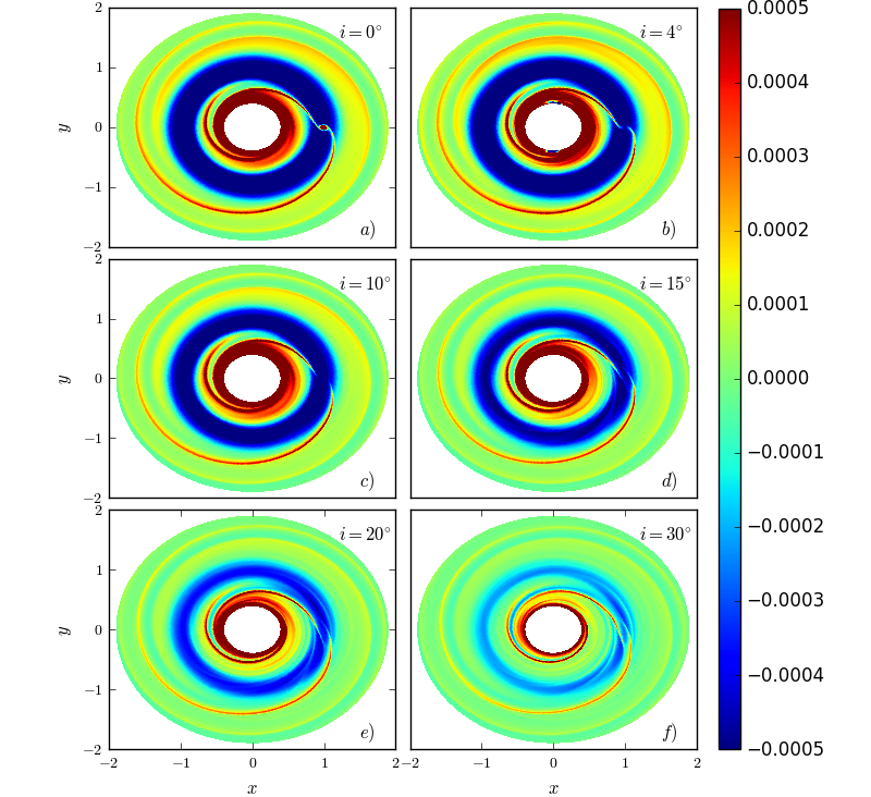
Figure 2: Perturbation of volume density $(\rho-\rho_{i})$ at $z=0$ after $t=200$ orbits, for different inclinations. In all cases, $q=10^{-3}$, $h=0.05$, and $\nu=10^{-5}$ (Runs 1 to 6). In all the plots, the planet is at $x=\cos i$, $y=0$ and $z=\sin i$, i.e. it is at its maximum height from the disc. Note that the scale is linear (not logarithmic).

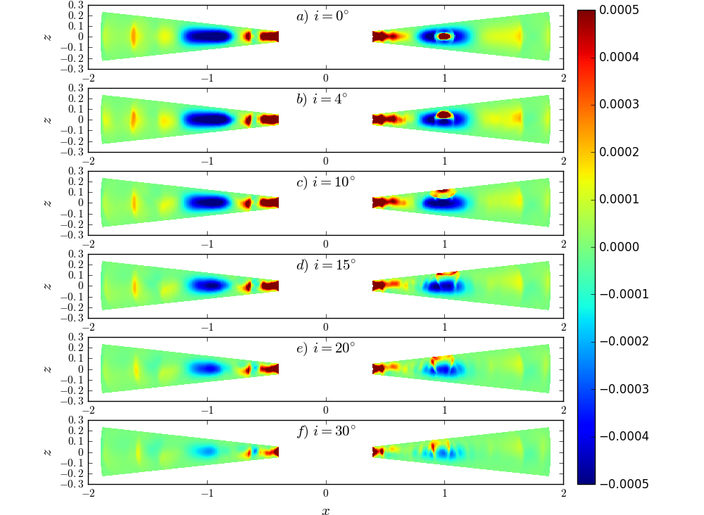
Figure 3: Same as Figure 2 but along vertical cross sections in the plane $y=0$.

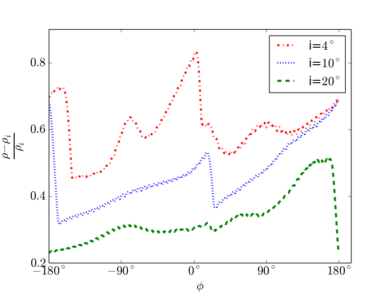
Figure 4: Perturbation of volume density along the crest of the outer spiral wave, at $z=0$.

4.1.2 Stationary gap profile in the approximation of local deposition of the torque

Under the assumption that the gravitational torque is locally (instantaneously) deposited in the disc (i. e. ignoring the propagation of waves before damping) a steady state is reached when the gravity is balanced by the viscous torque at every ring of the disc (see, for instance, Varnière et al., 2004; Crida et al., 2006). The radial densities of the viscous torque, $dT_{\nu}/dR$, and of the gravitational torque, $dT_{g}/dR$ can be obtained from Equations (4) and (22). Then, equating these torque densities, we obtain a differential equation that describes the gap structure:

$$\frac{1}{\Sigma}\frac{d\Sigma}{dR}=\frac{\xi}{3\pi\nu R^{2}\Omega\Sigma}\frac{dT_{g}}{dR}-\frac{1}{2R}.$$ (30)

To solve Equation (30), we need to choose the boundary condition. In the outer parts of the disc, far away from the planet, we expect that the surface density remains essentially unperturbed. Thus, it is ordinary to integrate Equation (30) from a certain point $R_{\rm max}\gg R_{p}$ inwards down to $R_{p}+r_{\rm min}$, where $r_{\rm min}$ is the distance from the planet where the impulse approximation breaks down. We may continue the integration of the equation in the inner disc by adopting a reasonable value for $\Sigma$ at $R_{p}-r_{\rm min}$. For instance, Crida et al. (2006) assumed that $\Sigma(R)\propto R^{-1/2}$ between $R_{p}-r_{\rm min}$ and $R_{p}+r_{\rm min}$, and adopted $r_{\rm min}=2R_{H}$, with $R_{H}$ the Hill radius.

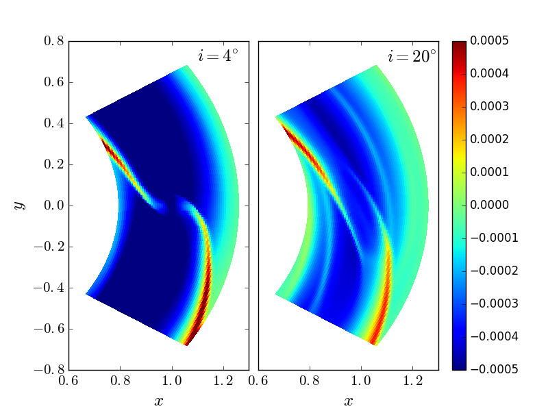
Figure 5: Zoom of the perturbed density $\rho-\rho_{i}$ at $z=0$ and $t=200$ orbits, for inclinations $i=4^{\circ}$ (Run 2) and $i=20^{\circ}$ (Run 5). The planet is at $x=0.9975$, $y=0$ and $z=0.0697$ in the left panel and at $x=0.9396$, $y=0$ and $z=0.3420$ in the right panel.

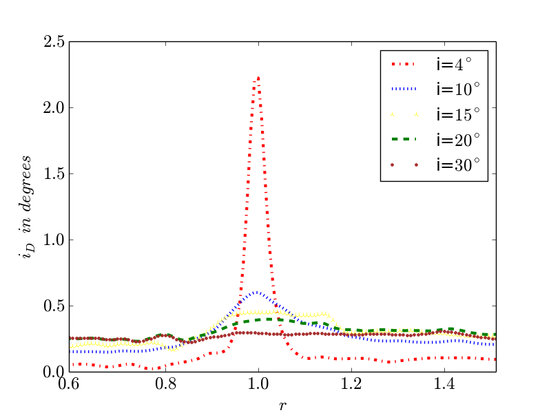
Figure 6: Inclination angle of the disc, $i_{D}$, as a function of $r$ after $200$ orbits, for $q=10^{-3}$, $h=0.05$ and different $i$. The rms in the measurement of $i_{D}$ is $0.05^{\circ}$. Thus, $i_{D}$ values below $\sim 0.05^{\circ}$ are not significant.

In the coplanar case, the resultant gap profile using the instantaneous damping approximation (i.e. using Eq. 30) has been extensively studied. It was found that the predicted gap profile is consistent with the simulated gaps only for high disc viscosities. At lower viscosities, the predicted gaps are wider than those observed in numerical simulations (for instance, see Varnière et al., 2004; Crida et al., 2006). Moreover, at these low viscosities the predicted scaling relation between the surface density averaged over the bottom of the gap ($\Sigma_{\rm gap}$) and $q$ is also incorrect; it cannot explain why $\Sigma_{\rm gap}$ scales as a power-law with $q$, as found in numerical simulations (e.g., Duffell et al., 2014; Fung et al., 2014).

4.1.3 Gap depth in a zero-dimensional analysis

In order to reproduce the dependence of gap depth on $q$, viscosity and $h$ observed in hydrodynamical simulations for the coplanar case, Fung et al. (2014), Kanagawa et al. (2015) and Duffell (2015) have invoked a “zero-dimensional” approximation, which assumes that the torque occurs only within the width of the gap. Under this approximation, the total one-sided torque can be written as

$$T_{g}=\hat{f}_{0}(i,h)q^{2}\Sigma_{\rm gap}R_{p}^{4}\omega^{2}h^{-3}.$$ (31)

By choosing reasonable values for $l_{\rm min}$ and $l_{\rm max}$, the scaling of the prefactor $\hat{f}_{0}$ with $i$ and $h$ can be computed from Equations (22) and (24). As discussed in §3.2, we take $l_{\rm min}={\rm max}\{(q/3)^{1/3},h\}$ and $l_{\rm max}=1$. For a fixed aspect ratio $h_{0}$, we can find how $\hat{f}_{0}$ depends on the inclination $i$. To do so, we have evaluated the integral given in Equation (24) for $l_{\rm min}=1.1h$, $l_{\rm max}=1$, and different inclinations. For the particular value of $h=0.05$, we find that $\hat{f}_{0}(i,h=0.05)$ can be fitted as

$$\hat{f}_{0}(i,h=0.05)= 0.744\exp\left(-\frac{i}{3}\right)-0.450\exp\left(-0.7i\right)$$ (32)

$$+0.155\exp\left(-\frac{i^{0.9}}{5.6}\right)+0.0004,$$

where $i$ is the inclination angle in degrees. This fit is valid for $i<35^{\circ}$, with a fractional error lower than $4\%$. For the calibration of the magnitude of $\hat{f}_{0}$ (i.e., to fix the value of $\xi$), we have used the condition that $\hat{f}_{0}=0.45$ for $i=0$ (see §2). It is worth noting that $\hat{f}_{0}$ decays a factor of $100$ between $i=0$ and $i=30^{\circ}$.

Once $\hat{f}_{0}$ is determined, Duffell’s model predicts $\Sigma_{\rm gap}$ through the formula

$$\frac{\Sigma_{\rm gap}}{\Sigma_{0}}=\left(1+\frac{\hat{f}_{0}q^{2}R_{p}^{2}\omega}{3\pi\nu h^{3}}\right)^{-1}.$$ (33)

Duffell (2015) also provides a recipe to obtain the profile of the gap. However, the calculation of the profile requires knowledge of the angular momentum flux due to the damping of the planetary wake, which is uncertain for planets in inclined orbits. Therefore, we only use the “zero-dimensional analysis” to predict the gap depth.

4.2 The formation of the gap in the local approximation: time evolution and inclination damping

The steady-state gap formed by a coplanar planet has been studied in great detail because the timescale to reach the steady state is shorter than the migration timescale (see §2). For a planet on an inclined orbit, the inclination damping timescale may be comparable to or smaller than the timescale for gap opening if the disc is sufficiently massive (Marzari & Nelson, 2009; Xiang-Gruess & Papaloizou, 2013; Bitsch et al., 2013). Under these circumstances, it is necessary to consider the time evolution of the disc surface density in order to include the dependence of the planet’s inclination with time.

Suppose that $i(t)$ is known. Then, the torque density $dT_{g}/dR$ depends implicitly on time through $i(t)$. Assuming that the evolution of the disc is axisymmetric, $\Sigma(R,t)$ can be computed by solving the continuity equation

$$\frac{\partial\Sigma}{\partial t}+\frac{1}{R}\frac{\partial}{\partial R}(R\Sigma v_{\mbox{{\tiny$R$}}})=0,$$ (34)

the radial momentum equation

$$\frac{\partial v_{\mbox{\tiny$R$}}}{\partial t}+v_{\mbox{\tiny$R$}}\frac{\partial v_{\mbox{\tiny$R$}}}{\partial R}=-\frac{GM_{S}}{R^{2}}+\frac{v_{\phi}^{2}}{R}-\frac{1}{\Sigma}\frac{\partial}{\partial R}(\Sigma c_{s}^{2}),$$ (35)

and the conservation of angular momentum

$$\frac{\partial L}{\partial t}+\frac{1}{R}\frac{\partial}{\partial R}(Rv_{\mbox{\tiny$R$}}L)=\frac{\nu}{R}\frac{\partial}{\partial R}(\Sigma R^{3}\Omega^{\prime})+\frac{\xi}{2\pi R}\frac{dT_{g}}{dR},$$ (36)

where $\Omega\equiv v_{\phi}/R$, $\Omega^{\prime}\equiv d\Omega/dR$ and $L\equiv\Sigma\Omega R^{2}$ is the angular momentum of a differential ring in the disc (e.g., Pringle 1981). In Equation (36), we have employed the local deposition approximation.

As a particular case, one can derive the time evolution of $\Sigma(R,t)$ in the presence of a planet on a fixed orbit, i.e. $i(t)=i_{0}=$const, in a disc that initially has no gap. To test whether the present 1D model is successful or not, it is sufficient to check if $\Sigma(R,t)$ obtained in full 3D hydrodynamical simulations is correctly reproduced for any value of $i_{0}$. If so, the formalism should also satisfactorily predict $\Sigma(R,t)$ for an arbitrary function $i(t)$.

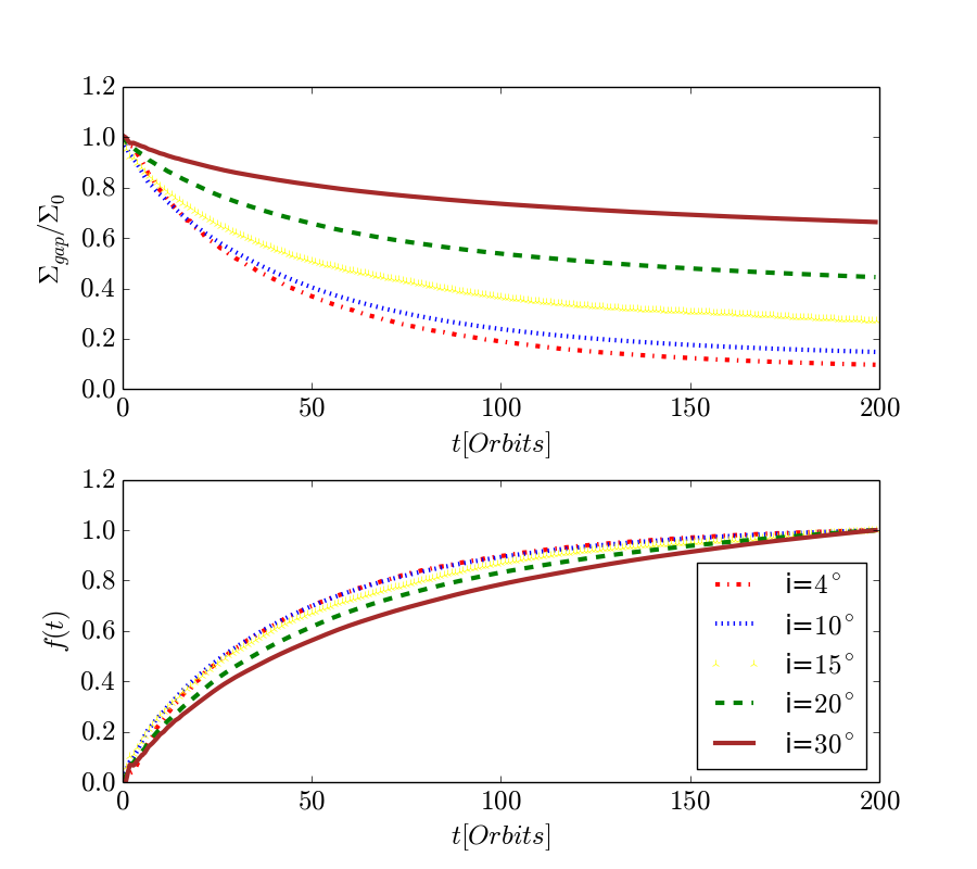
Figure 7: Temporal evolution of $\Sigma_{\rm gap}$ for different inclinations. In all cases $q=10^{-3}$ and $h=0.05$.

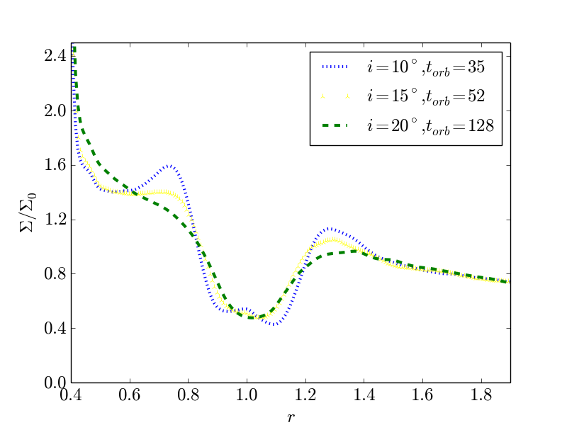
Figure 8: Radial profiles of the azimuthally averaged surface density $\Sigma$ at the time when $\Sigma_{\rm gap}=\Sigma_{0}/2$. The corresponding time depends on inclination $i$ and is quoted at the corner of the figure.

Figure 9: Gap profiles using the local damping approximation (see §4.2) with $\xi=1$ (dotted lines) and $\xi=2$ (dashed lines) together with those from numerical simulations (solid lines) after $45$ and $200$ orbits, for different inclinations. The stationary gap profiles using the local damping approximation are displayed in the right column. In all cases $q=10^{-3}$ and $h=0.05$.

Figure 10: Comparison between the gap profiles in the simulations with $i=20^{\circ}$ and different $q$ (solid lines) with those using the local damping approximation with $\xi=2$ (dashed lines). In all cases $h=0.05$.

Table 1: Parameters of the simulations. $q_{\rm crit}$ is the viscous critical value for gap formation according to Eqs (25)-(29). In all the cases, the kinematic viscosity is $10^{-5}$. Remind that $q$ denotes the planet to star mass ratio.

Run	$i$	$h$	$q_{\rm crit}/10^{-3}$	$q/10^{-3}$	$\Sigma_{\rm gap}/\Sigma_{0}$
	deg				at $200$ orbits
1	0	0.05	$0.5$	$1$	0.093
2	4	0.05	$0.55$	$1$	0.097
3	10	0.05	$0.8$	$1$	0.148
4	15	0.05	$1.2$	$1$	0.273
5	20	0.05	$1.8$	$1$	0.445
6	30	0.05	$3.0$	$1$	0.664
7	15	0.05	$1.2$	$3$	0.011
8	20	0.05	$1.8$	$3$	0.037
9	20	0.05	$1.8$	$0.3$	0.927
10	20	0.025	$1.8$	$1$	0.264

5 NUMERICAL SIMULATIONS

5.1 The code and initial conditions

In our study of the gap opening by a planet on inclined orbit, we use a spherical coordinate system $(r,\theta,\phi)$, where $r$ is the radial coordinate, $\theta$ is the polar angle, and $\phi$ is the azimuthal angle. The hydrodynamical equations describing the flow are the equation of continuity

$$\frac{\partial\rho}{\partial t}+\mbox{\boldmath$\nabla$}{}\cdot(\rho\mbox{\boldmath$v$}{})=0$$ (37)

and momentum equation

$$\frac{\partial\mbox{\boldmath$v$}{}}{\partial t}+(\mbox{\boldmath$v$}{}\cdot\nabla)\mbox{\boldmath$v$}{}=-\frac{1}{\rho}\mbox{\boldmath$\nabla$}{}P-\mbox{\boldmath$\nabla$}{}\Phi+\mathbf{f_{\nu}}.$$ (38)

Here $\rho$ is the density, $v$ the velocity, $\Phi$ is the gravitational potential and $\mathbf{f_{\nu}}$ represents the viscous force per unit volume. The disc is assumed to be locally isothermal, i.e. the pressure is given by

$$P=\rho c_{s}^{2},$$ (39)

where $c_{s}(r)$ is the isothermal sound velocity.

We use the hydrodynamic FARGO3D code (Benítez-Llambay & Masset, 2016) which is the successor of the hydrodynamic FARGO code. Both codes use the orbital advection algorithm of Masset (2000), which significantly increases the timestep in thin protoplanetary discs.

We use a reference frame centred on the star, and corotating with the planet. The gravitational potential $\Phi$ due to the central star and the planet is given by

$$\Phi=\Phi_{S}+\Phi_{p},$$ (40)

where

$$\Phi_{S}=-\frac{GM_{S}}{r},$$ (41)

and

$$\Phi_{p}=-\frac{GM_{p}}{\sqrt{r_{p}^{2}+\epsilon^{2}}}+\frac{GM_{p}r\cos\phi}{r_{p}^{2}},$$ (42)

where $r_{p}\equiv|\mbox{\boldmath$r$}{}-\mbox{\boldmath$R$}{}_{p}|$ is the distance from the planet, and $\epsilon$ is a softening length used to avoid computational problems arising from a divergence of the potential in the vicinity of the planet. We use $\epsilon=0.6H_{p}$, where $H_{p}$ is the disc scaleheight at $R=R_{p}$, but we also performed simulations with $\epsilon=0.3H_{p}$ to check that the results are not sensitive to the exact value of $\epsilon$. The last term in Equation (42) is the indirect term which appears because the reference frame is non-inertial and centred on the star. The self-gravity of the disc is ignored in our simulations.

In Runs 1 to 10, the planet, whose orbit is tilted by an angle $i$ with respect to the initial midplane of the disc, is forced to describe a circular orbit of radius $R_{p}$ around the central star. Thus, we ignore the changes in the orbital parameters of the planet caused by tidal torques (see §5.3 for simulations of a planet that is left to freely migrate because of the tidal torques). No accretion of gas by the planet is considered here.

The aspect ratio, $h\equiv H/r$, is assumed to be constant across the disc, where $H$ is the vertical scale height of the disc. The initial density of the disc, $\rho_{i}(R,z)$, is derived by assuming a power-law surface density

$$\Sigma_{i}(R)=\Sigma_{0}\left(\frac{R_{p}}{R}\right)^{1/2},$$ (43)

and by imposing hydrostatic equilibrium, which implies that $c_{s}(r)=hr\Omega$ where $\Omega(r)$ is the Keplerian angular velocity around the star. Note that $\Sigma_{0}$ denotes the initial surface density at $R=R_{p}$.

Our distance unit is $R_{p}$ and our time unit $\omega^{-1}$ (as defined in section 2, $\omega$ is the angular velocity of the planet). The period of the planet is therefore $2\pi$.

The domain of the simulations extends radially from $r=0.4$ to $r=2.5$. The polar angle $\theta$ covers $14^{\circ}$ (from $83^{\circ}$ to $97^{\circ}$) for the simulations with $h=0.05$ and $8^{\circ}$ (from $86^{\circ}$ to $94^{\circ}$) for discs with $h=0.025$. All the simulations have the same grid size $(N_{r},N_{\phi},N_{\theta})=(266,768,64)$.

In the radial direction, we implemented damping boundary conditions for the radial component of the velocity $v_{r}$ (de Val-Borro et al., 2006). More specifically, $v_{r}$ is artificially damped in the regions $r\in[0.4,0.5]$ and $r\in[2.1,2.5]$ by solving the equation

$$\frac{\partial v_{r}}{\partial t}=-\frac{\Omega}{2\pi}\left(v_{r}-v_{r0}\right)\chi(r)$$ (44)

after each time-step. Here $v_{r0}$ is the radial velocity component at $t=0$ and $\chi(r)$ is a parabolic function which takes the value $1$ at the domain boundary and $0$ at the limit of the damping region (e.g., de Val-Borro et al., 2006). For the other two velocity components and the density we use reflecting boundary conditions without any damping.

5.2 Results

In this Section, we investigate numerically the interaction of an inclined planet with the disc. The parameters of the simulations for planets on fixed orbits are given in Table 1. In §5.3 we present a simulation for a freely moving planet. In most of our simulations, we take $q=10^{-3}$, $h=0.05$ and a kinematic viscosity $\nu=10^{-5}$.

5.2.1 Evolution of the disc: planets on fixed orbits

Here we study the formation and structure of the gap carved by a planet on a fixed inclined circular orbit for several inclinations $0^{\circ},4^{\circ},10^{\circ},15^{\circ},20^{\circ}$, and $30^{\circ}$ with respect to the initial midplane of the disc, which corresponds to the plane $\theta=90^{\circ}$. The simulations were run over $200$ planetary orbits. The strengh of the interaction between the planet and the disc depends on the inclination of the planetary orbit. For $h=0.05$, the aperture angle of the disc is $2.9^{\circ}$. For inclinations larger than $2.9^{\circ}$, the planet spends a fraction of its orbital period within the disc that decreases as the inclination increases. Figures 2 and 3 display the perturbation of volume density after $200$ orbits on equatorial and meridional cross sections, for $q=10^{-3}$, $h=0.05$, $\nu=10^{-5}$ and different inclinations. As occurs in the coplanar case, the planet triggers a wake with two spiral arms that emanate from the planet (see Figures 2$a$ and 3$a$). A gap in the surface density is also apparent. The gap divides the disc into two regions: $i)$ the inner disc, $r<R_{p}$, and the outer disc at $r>R_{p}$. In the inner (outer) disc, the spiral arm is leading (trailing), as in the non-inclined case. The amplitude of the spiral arms depends on the inclination of the planetary orbit as can be observed in the cases $a)-f)$ in Figure 2. Figure 4 shows the perturbed density along the crest of the outer spiral arm. It can be seen that for $i=4^{\circ}$ the density enhancement along the crest is three times greater than for $i=20^{\circ}$.

Since the timescale for gap opening is much larger than the dynamical timescale, the structure of the gap is rather axisymmetric (i.e. it does not depend on the phase of the planet), except in the vicinity of planet’s position. A magnification of the density map in a box centred at $x=X_{p}$, $y=Y_{p}$ and $z=0$ is shown in Figure 5. Note that the planet is at its maximum distance from the disc in these snapshots. We see that the higher inclination case has a less clean gap, and finer substructure. For $i=20^{\circ}$, the spiral waves do not emanate from the projected position of the planet.

The appearance of the gap of an inclined planet is somehow reminiscent of the aspect of HL Tau gap structures (ALMA Partnership et al., 2015, 2015a, 2015b, 2015c), in which we do not see local, conspicuous density enhancements at particular azimuth, which could potentially be due to planets. A large number of mechanisms can account for the existence of the gap structures observed in HL Tau (Carrasco-Gonzalez et al., 2009; Flock et al., 2015; Gonzalez et al., 2015; Zhang et al., 2015; Carrasco-Gonzalez et al., 2016; Okuzumi et al., 2016; Ruge et al., 2016; Yen et al., 2016). We simply mention that the lack of localized structures within the gap does not rule out planetary torques as the mechanism responsible for their existence, since a midly inclined planet does not trigger a large density enhancement at its projected location in the gap.

The tidal perturbation of a planet with non-zero inclination may lead to the excitation of vertical disturbances (bending waves or warps) in the disc (for a binary star, see, e.g., Papaloizou & Terquem, 1995; Larwood et al., 1996). For massive enough planets, the disc will try to realign with the orbital plane of the planet, reducing the relative inclination between planet’s orbit and the disc. In order to quantify the excitation of vertical modes (warps) in the disc, we calculated the inclination of the disc at different radii using the expression

$$i_{\textsc{\tiny D}}(r)=\arccos{\frac{L_{z}(r)}{\lvert\mbox{\boldmath$L$}{}(r)\rvert}},$$ (45)

where $\mbox{\boldmath$L$}{}(r)$ is the angular momentum vector of a differential ring of the disc:

$$\mbox{\boldmath$L$}{}(r)=\int\rho(\mbox{\boldmath$r$}{}\times\mbox{\boldmath$v$}{})\,d\theta\,d\phi.$$ (46)

For the adopted values of $q$, the disc hardly changes its inclination (Figure 6). The largest values of $i_{\textsc{\tiny D}}$ occur for the case $i=4^{\circ}$ and for rings having radii $\simeq R_{p}$. In particular, for $q=10^{-3}$, $h=0.05$ and $i=4^{\circ}$, these rings are displaced by an angle $\simeq 2^{\circ}$. For $i\geq 10^{\circ}$, $i_{\textsc{\tiny D}}$ is very small compared to $i$ and hence it is a good approximation to ignore the bend of the disc.

5.2.2 Scaling relations for the gap

As expected, the depth of the gap depends on the planetary inclination $i$. At low inclinations ($i<10^{\circ}$), the time for gap opening is shorter than in the case where the planet orbit is more inclined. As a measure of the depth, we determine $\Sigma_{\rm gap}$ from our simulations by calculating the surface density averaged over azimuth and over the radial direction between $R_{p}-\sqrt{2}R_{H}$ and $R_{p}+\sqrt{2}R_{H}$. Figure 7 displays $\Sigma_{\rm gap}$ as a function of time for Runs 1 to 6. The gap density $\Sigma_{\rm gap}(t)$ converges toward a constant value at larger time. In order to compare the rate of emptying of gas in the gap, we write

$$\Sigma_{\rm gap}(t)=\left[1-f(t)\right]\Sigma_{0}+f(t)\Sigma_{200},$$ (47)

where $\Sigma_{200}$ denotes the surface density in the gap at $t=200$ orbits and $f(t)$ is an auxiliary function that satisfies $f(0)=0$ and $f(200)=1$. If $f(t)$ becomes flat, it means that we have essentially reached the asymptotic value of $\Sigma_{\rm gap}$. As judged from Figure 7, the rate of depletion of gas in the gap is very low after $200$ orbits, indicating that $\Sigma_{200}$ may be considered as representative of the asymptotic value, except perhaps for the simulation with $i=30^{\circ}$. In fact, the gap cleaning proceeds slightly slower for high $i$ (lower panel in Figure 7).

In order to compare how the process of gap opening occurs for different planetary inclinations, we plot the azimuthally-averaged surface density of the gap at the time when the condition $\Sigma_{\rm gap}=\Sigma_{0}/2$ is satisfied (Figure 8). For $i=4^{\circ},10^{\circ},15^{\circ}$, and $20^{\circ}$ this occurs at $25$, $40$, $50$, and $109$ orbits, respectively. In the case $i=30^{\circ}$, the planet is unable to carve such a deep gap during the time of the simulation ($200$ orbits); at the end of this simulation $\Sigma_{\rm gap}=0.67\Sigma_{0}$. We see that at the time when $\Sigma_{\rm gap}=\Sigma_{0}/2$, the profile of the gaps are clearly different. For $i=4^{\circ}$, the planet satisfies the condition $\Sigma_{\rm gap}=\Sigma_{0}/2$ in a shorter timescale and, moreover, it depletes more material, leading to a wider gap, than planets with larger inclinations. This means that the gap cleaning is more efficient, along a wider radial range, for low inclination planets. Also, the local maxima of the density that appear near the edges of the evacuated gap have more time to spread by viscous diffusion, since the plots of larger $i$ are made at a later time.

For each simulation, Table 1 lists the values of $q_{\rm crit}$, as derived in §4.1.1. We see that the viscous criterion for gap formation is roughly satisfied, in the sense that when $q>q_{\rm crit}$ it holds that $\Sigma_{200}\lesssim 0.2\Sigma_{0}$.

Figure 9 shows the radial profile of the azimuthally-averaged surface density after $45$ and $200$ planetary orbits and different inclination angles (but having the same kinematic viscosity and aspect ratio). It is apparent that the depth of the gap decreases with the inclination angle of the planet’s orbit. The surface density bumps at $r=1.4$ at $t=45$ and $t=200$ orbits appear because the profiles of the surface density are not completely relaxed at $t\leq 200$ orbits given that the viscous timescale is $\sim 2.5\times 10^{3}$ orbits.

We have compared the resultant gap profiles in the simulations with those predicted using the 1D model (the method described in §4.2), which assumes that the wake’s torque is deposited locally in the disc. We use $l_{\rm min}=(q/3)^{1/3}$ (see §3.2) and explore two values for $\xi$ ($\xi=1$ and $\xi=2$). We also plot the steady-state gap profile by integrating numerically Equation (30), with the boundary condition $\Sigma(2.5)=\Sigma_{0}/\sqrt{2.5}$, which is the unperturbed surface density at $R=2.5R_{p}$, and using $r_{\rm min}=R_{H}$.

To be fully satisfactory, the models should be able to reproduce the width and depth of the gap at any time. From Figure 9, we see that the width of the gaps is fairly reproduced for both $\xi=1$ and $\xi=2$. However, models with $\xi=1$ predict shallower gaps than those found in the simulations for inclinations $\geq 10^{\circ}$. It is remarkable that the depth of the gaps at $200$ orbits in the full 3D simulations is larger than the depth of the stationary gaps in the 1D model, i.e. the ‘steady state’ curves in Figure 9. This suggests that the value of $\xi$ is larger than $1$. This is not unexpected if one reminds that the torque calculated by summing the contribution from all Lindblad resonances in the coplanar case is a factor of $2.8$ larger than the torque calculated with the impulse approximation [see §2 and Lin & Papaloizou (1986a)].

Adopting $\xi=2$, there is a good level of agreement between the gap profiles derived using the 1D model and those found in the simulations for inclinations between $10^{\circ}$ and $20^{\circ}$ (see Figure 9). For lower inclinations ($i<10^{\circ}$), the 1D model overestimates the depth of the gap when assuming our fiducial value of $l_{\rm min}$ (not shown). In order to reproduce the gap profile found in the simulation with $i=4^{\circ}$, we need $l_{\rm min}=1.8(q/3)^{1/3}$.

For $i=30^{\circ}$, the 1D model clearly underestimates the depth of the gap at any time (Figure 9), indicating that at least one of our assumptions is not fully correct. It is plausible that for inclinations as large as $30^{\circ}$, the impulse approximation underestimates the torque. Moreover, the local damping approximation is less justified as the inclination increases because the perturbed density in the wake decreases (Figure 4). However, it is unclear that the resulting angular momentum flux driven by spiral arms will increase gap clearing in the vicinity of the planet.

In order to explore a bit further the 1D model, Figure 10 compares the gap profiles in our full 3D simulations with those in 1D models for $i=20^{\circ}$ and two different values of $q$. We see that for $q=3\times 10^{-3}$, the 1D model is still successful in reproducing the gap profile. However, for $q=3\times 10^{-4}$, the evacuation of gas from the gap is more efficient in the full 3D simulations than in the 1D models.

It is worthwhile to consider the predictions using the ‘zero-dimensional’ approximation. Following the procedure described in Section 4.1.3, we have calculated $\hat{f}_{0}(i,h)$ for $l_{\rm min}=0.87h,1.1h$ and $1.2h$. Figure 11 compares $\Sigma_{\rm gap}$ calculated using Equation (33) with the values obtained in the simulations. The general trend that the gap is shallower when increasing $i$ is consistent with simulations. A value for $l_{\rm min}$ of $1.2h$ is required to reproduce the gap density values for a disc with aspect ratio $=0.05$.

It is worthwile to look at Run 10. This simulation has $h=0.025$ and lies in the deeply nonlinear regime. For this run, the zero-dimensional approximation with $l_{\rm min}=1.2h$ predicts $\Sigma_{200}/\Sigma_{0}=0.38$, while the simulated disc has a gap with $\Sigma_{200}/\Sigma_{0}=0.26$. This illustrates that hydrodynamical effects may be important for very thin discs.

Figure 11: Predicted values of $\Sigma_{200}/\Sigma_{0}$ using the zero-dimensional approach (see §4.1.3) with $l_{\rm min}=0.87h$ (dotted lines), $l_{\rm min}=1.1h$ (dashed lines) and $l_{\rm min}=1.2h$ (solid lines), together with the values from the numerical simulations (symbols) for simulations with different inclinations (Run 1 to Run 6; top panel) and for simulations with different $q$ (Runs 5, 8 and 9; bottom panel).

5.3 Radial migration and inclination damping for free planets

In the impulse approximation, it is possible to estimate the characteristic timescales for radial migration and inclination damping for planets with inclination large enough that they cross the disc at supersonic velocities. Rein (2012) find that the inclination and the semimajor axis damping timescales, measured in units of the orbital period, are

$$\tau_{\rm inc}\equiv i/(2|di/dt|)=\frac{M_{S}}{2\pi q\Sigma_{0}R_{p}^{2}}\frac{i\sin^{3}(i/2)}{\ln\Lambda},$$ (48)

$$\tau_{\rm R}\equiv R_{p}/(2|\dot{R}_{p}|)=\frac{M_{S}}{8\pi q\Sigma_{0}R_{p}^{2}}\frac{\sin(i/2)\sin(i)}{\ln\Lambda},$$ (49)

where $\Sigma_{0}$ is the surface density of the disc at the intersection of the planetary orbit with the disc, and $\ln\Lambda$ is the Coulomb logarithm of the interaction. More specifically, $\Lambda$ is the ratio between the upper ($r_{\rm max}$) and lower ($r_{\rm min})$ cut-off length scales of the interaction. A similar formula (except by a factor of $2$) for the timescale for the orbit to change was derived by Xiang-Gruess & Papaloizou (2013). The timescales $\tau_{\rm inc}$ and $\tau_{\rm R}$ depend on the unperturbed local surface density of the disc, $\Sigma_{0}$, because it was assumed that the timescale for gap opening is larger than both $\tau_{\rm inc}$ and $\tau_{\rm R}$. If the planet is able to open a gap, the depletion of material in the planet vicinity should be taken into account. Once the planet has carved a gap, the rates of damping in $i$ and $R$ are expected to decrease (e.g., Xiang-Gruess & Papaloizou, 2013).

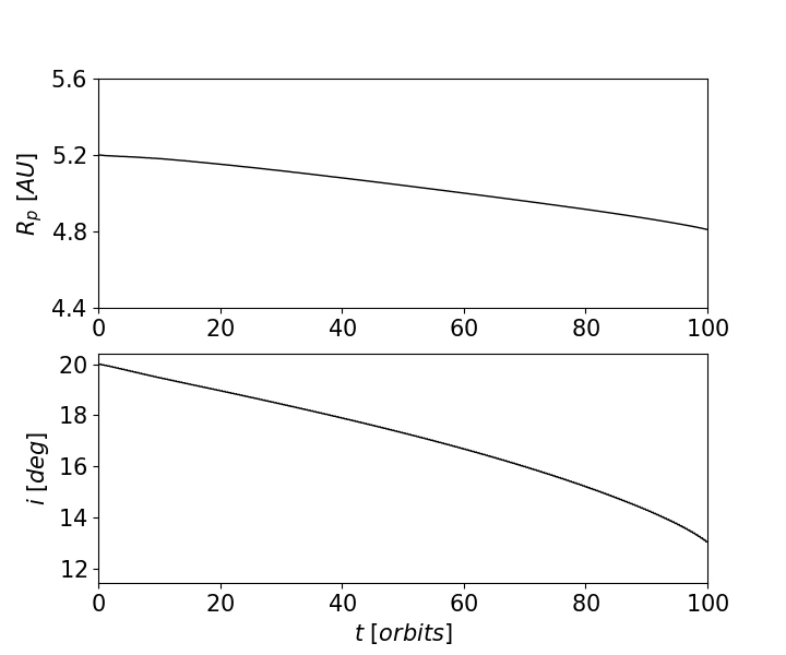
Figure 12: Top: Semimajor axis $R_{p}$ as function of time for a planet with $q=10^{-3}$ and an initial inclination of $i_{0}=20^{\circ}$. The disc has $\Sigma_{0}=210$ g cm^-2. Bottom: Temporal evolution of the planetary inclination $i$.

The timescale for inclination damping may be comparable or even smaller than the timescale for gap opening if the disc is sufficiently massive. For illustration, consider a planet-star system with $q=10^{-3}$, $M_{S}=1M_{\odot}$ and $i=20^{\circ}$. For these parameters, $\tau_{\rm inc}$ is given by

$$\tau_{\rm inc}=\frac{450}{\ln\Lambda}\left(\frac{\Sigma_{0}}{200\,{\rm g\,cm}^{-2}}\right)^{-1}\left(\frac{R_{p}}{5.2\,{\rm AU}}\right)^{-2}\,\,{\rm orbits}.$$ (50)

Since the timescale to form a gap with a depth $\Sigma_{\rm gap}=0.5\Sigma_{0}$ is $128$ orbits (see Figure 8), the inclination damping timescale is comparable to or smaller than the gap opening timescale if $\Sigma_{0}\gtrsim 600/\ln\Lambda$ g cm^-2 (assuming $R_{p}=5.2$ AU, $i=20^{\circ}$ and $q=10^{-3}$). The critical surface density is expected to increase linearly with $q$ because $\tau_{\rm inc}\propto q^{-1}$, whereas the timescale for gap opening goes as $\sim q^{-2}$.

In order to test these estimates, we perform one simulation in which the planet feels the tidal torques by the disc since the beginning of the simulation. The planet is initially in a circular orbit with $R_{p}=5.2$ AU and $i_{0}=20^{\circ}$. It has $q=10^{-3}$ and a softening radius $\epsilon=0.3H_{p}$. The initial surface density at $5.2$ AU is $210$ g cm^-2. Figure 12 shows the temporal evolution of $R_{p}$ and $i$. In $100$ orbits, the semimajor axis decays from $5.2$ AU to $4.8$ AU and the inclination from $20$ to $13$ deg, resulting in $di/dt=-0.07$ deg/orbit and $dR_{p}/dt=-4\times 10^{-3}$ AU/orbit. These rates of inclination damping and radial migration are consistent with those found in previous studies (Marzari & Nelson, 2009; Xiang-Gruess & Papaloizou, 2013). For instance, for a planet with $i_{0}=20^{\circ}$, $\Sigma_{0}=76$, and $q=10^{-3}$, Xiang-Gruess & Papaloizou (2013) find that $di/dt=-0.028$ deg/orbit and $dR_{p}/dt=-0.9\times 10^{-3}$ AU/orbit.

In order to compare with the predictions of Equations (48)-(49), we need to estimate $\ln\Lambda$ in our simulation. To do so, we use that $r_{\rm min}$ depends on the softening radius $\epsilon$ as $r_{\rm min}\simeq 2.25\epsilon=0.67H_{p}$ (Bernal & Sánchez-Salcedo, 2013) and that $r_{\rm max}\simeq 2.1\sqrt{2}H_{p}$ in a disc (Cantó et al., 2013; Xiang-Gruess & Papaloizou, 2013). Hence, we find that $\ln\Lambda\simeq 1.5$. Using this value, Equations (48) and (49) predict $di/dt=-0.027$ deg/orbit and $dR_{p}/dt=-0.9\times 10^{-3}$ AU/orbit. These values are a factor of $3-4$ smaller than those found in the simulations. Nevertheless, it is likely that the accuracy is better for larger inclinations (Rein, 2012; Xiang-Gruess & Papaloizou, 2013).

Given that the inclination damping timescale is comparable to the timescale for gap clearing, the process is dynamical in the sense that the inclination cannot be assumed to be constant. Figure 13 plots the surface density profile after $82$ orbits, that is, when the planet has an inclination of $15^{\circ}$, together with the surface density profile in simulations where the planets are at fixed orbits with inclinations $15^{\circ}$ and $20^{\circ}$. As expected, the surface density has its minimum at a inner radius when the planet is allowed to migrate. In addition, for the planet starting with $i_{0}=20^{\circ}$, the depth of the gap is larger when the planet is free to migrate than when the planet is forced to orbit at constant inclination ($20^{\circ}$). However, the planet that is forced to orbit at a constant inclination of $15^{\circ}$ opens a deeper gap after $82$ orbits than the gap produced by the migrating planet.

We conclude that for planets with masses of the order of $M_{J}$ and for $\Sigma_{0}\gtrsim 100$ g cm^-2, the inclination damping timescale is comparable to or shorter than the gap clearing process and, therefore, it is necessary to solve the time-dependent 1D model described in §4.2. For those values of $\Sigma_{0}$, the inclination is damped to zero in a timescale much shorter than the lifetime of the disc. Therefore, the scattering process of inclined planets should occur when the surface density of the disc was significantly smaller than $100$ g cm^-2 (see also Bitsch et al., 2013).

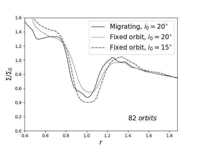
Figure 13: Comparison of the radial profiles of the surface density for migrating and non-migrating planets, after $82$ orbits.

6 Conclusions

We have developed a model to understand the dynamical response of a protoplanetary disc to the presence of a planet in inclined orbit. We considered planets massive enough to open a gap but not too massive to warp the disc significantly. Given that the impulse approximation for non-inclined planets yields correct scalings and better than a factor of $2$ estimates of the torque (e.g. Lin & Papaloizou, 1993; Armitage, 2010), we have computed the excitation torque density by inclined planets on circular orbits in the impulse approximation. Using this simple approach, we have derived a viscous criterion for the formation of gaps by mildly inclined planets ($i\leq 30^{\circ}$) [see §4.1.1]. Such a criterion may be useful when the planet has acquired its inclination after the gas in the disc is well depleted, or to interpret simulations that are started after the disc has evolved with the planet at a fixed, constant inclination.

For planets that are forced to describe fixed circular orbits, we have calculated the temporal evolution of the gap profile in the impulse approximation and using the hypothesis of local damping. We have compared these radial gap profiles with those derived in 3D hydrodynamical simulations. The simple model underestimates the depth of the gap for $i\geq 10^{\circ}$ when comparing with the results of our simulations. Introducing a correction factor of $2$ in the torque allows us to reproduce successfully the temporal evolution of the gap profile for inclinations between $10^{\circ}$ and $20^{\circ}$, and planetary masses $\geq 1M_{J}$. For planetary inclinations larger than $20^{\circ}$, the simple model underestimates the depth of the gap probably because one assumption on which the impulse approximation is based, namely that the interaction is local, is only poorly verified at large inclinations.

We have also computed the depth of the stationary gap in the so-called zero-dimensional approximation and find that it accounts correctly the trend of the gap depth with the inclination and mass of the planet.

In order to check the validity of the approximations made in our approach, we have mainly focused on planets in fixed circular orbits. This approximation is strictly valid only if the inclination damping timescale is larger than the timescale for gap opening. Nevertheless, for given, arbitary functions $i(t)$, our formalism allows to derive the gap profile as a function of time. The results will be most accurate for $10^{\circ}\leq i(t)\leq 20^{\circ}$.

Appendix A The prograde, coplanar orbit as a particular case

In the following, we specialize the equations given in §3 for the case $i=0$ and $\varepsilon=1$. Equations (12) and (14) reduce to:

$$\mbox{\boldmath$d$}{}_{\rm min}=\begin{pmatrix}[R_{d}-R_{p}]\cos\phi_{p}\\ [R_{d}-R_{p}]\sin\phi_{p}\\ 0\end{pmatrix},$$ (51)

and

$$\mbox{\boldmath$v$}{}_{\rm rel}=R_{p}\begin{pmatrix}[\omega-\Omega]\sin\phi_{p}\\ [\Omega-\omega]\cos\phi_{p}\\ 0\end{pmatrix},$$ (52)

respectively. Clearly, we have that $d_{\rm min}=|R_{d}-R_{p}|$ and $v_{\rm rel}=R_{p}|\omega-\Omega|$.

According to Equation (22) with $i=0$, the torque in an elementary ring is

$$\frac{dT_{g}(l)}{dR}=\frac{3\Sigma(R)\omega^{2}R_{p}^{3}|l|}{4\pi}\int_{0}^{2\pi}({\mathcal{R}}_{1}\tilde{\mbox{\boldmath$v$}{}}_{\rm rel})\cdot\mbox{\boldmath$e$}{}_{\phi}\,d\phi_{p}.$$ (53)

Remind that $|l|=|R_{d}-R_{p}|/R_{p}$, and ${\mathcal{R}}_{1}={\mathcal{R}}-{\mathcal{I}}$, where ${\mathcal{R}}$ is the rotation matrix of angle $\delta_{e}$ around the direction of the vector $\mbox{\boldmath$d$}{}_{\rm min}\times\mbox{\boldmath$v$}{}_{\rm rel}$. For the coplanar case ($i=0$) and for a Keplerian disc, the rotation is around the vector $-\mbox{\boldmath$e$}{}_{z}$, and the rotation matrix is given by

$${\mathcal{R}}=\left(\begin{array}[]{ccc}\cos\delta_{e}&\sin\delta_{e}&0\\ -\sin\delta_{e}&\cos\delta_{e}&0\\ 0&0&1\end{array}\right).$$ (54)

For small values of $\delta_{e}$, we have

$${\mathcal{R}}_{1}=\delta_{e}\left(\begin{array}[]{ccc}-\delta_{e}/2&1&0\\ -1&-\delta_{e}/2&0\\ 0&0&0\end{array}\right),$$ (55)

and, consequently

$$({\mathcal{R}}_{1}\tilde{\mbox{\boldmath$v$}{}}_{\rm rel})\cdot\mbox{\boldmath$e$}{}_{\phi}=\frac{\omega-\Omega}{\omega}\frac{\delta_{e}^{2}}{2}.$$ (56)

On the other hand, the deflection angle is

$$\delta_{e}=\frac{4G^{2}M_{p}^{2}}{v_{\rm rel}^{4}d_{\rm min}^{2}}=4q^{2}\left(\frac{\omega}{\omega-\Omega}\right)^{4}\left(\frac{R_{p}}{R_{d}-R_{p}}\right)^{2}.$$ (57)

Substituting into Equation (56) and using that $\omega-\Omega\simeq 3\omega(R_{d}-R_{p})/(2R_{p})$, we get

$$({\mathcal{R}}_{1}\tilde{\mbox{\boldmath$v$}{}}_{\rm rel})\cdot\mbox{\boldmath$e$}{}_{\phi}=\frac{16}{27}q^{2}\left(\frac{R_{p}}{R_{d}-R_{p}}\right)^{5},$$ (58)

and substituing into Equation (53) we finally obtain

$$\frac{dT_{g}}{dR}=\pm\frac{8}{9}q^{2}\Sigma R_{p}^{3}\omega^{2}\left(\frac{R_{p}}{R_{d}-R_{p}}\right)^{4},$$ (59)

or

$$\frac{dT_{g}}{dR}=\pm\frac{8}{9}q^{2}\Sigma R_{p}^{3}\omega^{2}\left(\frac{R_{p}}{\Delta}\right)^{4},$$ (60)

where the positive sign is for the external disc ($R_{d}>R_{p}$) and the minus sign is for the internal disc ($R_{d}<R_{p}$). Integrating the above equation over $\Delta$ between $\Delta_{0}$ and $\infty$, we obtain

$$T_{g}=\pm\frac{8q^{2}\Sigma R_{p}^{4}\omega^{2}}{27}\left(\frac{R_{p}}{\Delta_{0}}\right)^{3}.$$ (61)

We have recovered the same formula as given in Lin & Papaloizou (1993) (their equation 5).

References

- Albrecht et al. (2012) Albrecht S. et al., 2012, ApJ, 757, 18
- ALMA Partnership et al. (2015) ALMA Partnership, Fomalont, E. B., Vlahakis C., et al., 2015, ApJ, 808, L1
- ALMA Partnership et al. (2015a) ALMA Partnership, Hunter, T. R., Kneissl R., et al., 2015a, ApJ, 808, L2
- ALMA Partnership et al. (2015b) ALMA Partnership, Brogan, C. L., Perez L. M., et al., 2015b, ApJ, 808, L3
- ALMA Partnership et al. (2015c) ALMA Partnership, Vlahakis C., Hunter T. R., et al., 2015c, ApJ, 808, L4
- Armitage (2010) Armitage P. J. 2010, Astrophysics of planet formation, Cambridge University Press
- Baruteau & Masset (2013) Baruteau C., Masset F. 2013, Lecture Notes in Physics, Vol. 861, Tides in Astronomy and Astrophysics, Springer-Verlag, Berlin, p. 201
- Benítez-Llambay & Masset (2016) Benítez-Llambay P., Masset F. S. 2016, ApJS, 223, 11
- Bernal & Sánchez-Salcedo (2013) Bernal C. G., Sánchez-Salcedo F. J. 2013, ApJ, 775, 72
- Bitsch & Kley (2011) Bitsch B., Kley W. 2011, A&A, 530, 41
- Bitsch et al. (2013) Bitsch B., Crida A., Libert A.-S., Lega E. 2013, A&A, 555, 124
- Bryden et al. ( 1999) Bryden G., Chen X., Lin D. N. C., Nelson R. P., Papaloizou J. C. B. 1999, ApJ, 514, 344
- Cantó et al. (2013) Cantó J., Esquivel A., Sánchez-Salcedo F. J., Raga A. C. 2013, MNRAS, 762, 21
- Carrasco-Gonzalez et al. ( 2009) Carrasco-Gonzalez C., Rodriguez L. F., Anglada G., Curiel S. 2009, ApJ, 693, L86
- Carrasco-Gonzalez et al. ( 2016) Carrasco-Gonzalez C., et al. 2016, ApJ, 821, L16
- Cresswell & Nelson (2006) Cresswell P., Nelson R. P. 2006, A&A, 450, 833
- Cresswell et al. ( 2007) Cresswell P., Dirksen G., Kley W., Nelson R. P. 2007, A&A, 473, 329
- Crida et al. ( 2006) Crida A., Morbidelli A., Masset F. 2006, Icarus, 181, 587
- de Val-Borro et al. ( 2006) de Val-Borro M. et al. 2006, MNRAS, 370, 529
- Duffell et al. ( 2014) Duffell P. C., Haiman Z., MacFadyen A. I., D’Orazio D. J., Farris B. D. 2014, ApJ, 792, L10
- Duffell (2015) Duffell P. C. 2015, ApJ, 807, L11
- Fabrycky & Winn (2009) Fabrycky D. C., Winn J. N. 2009, ApJ, 696, 1230
- Flock et al. ( 2015) Flock M., Ruge J. P., Dzyurkevich N., Henning Th., Klahr H., Wolf S. 2015, A&A, 574, A68
- Fung et al. ( 2014) Fung J., Shi J.-J., Chiang E. 2014, ApJ, 782, 88
- Goldreich & Tremaine (1980) Goldreich P., Tremaine S. 1980, ApJ, 241, 425
- Gonzalez et al. (2015) Gonzalez J. F., Laibe G., Maddison S. T., Pinte C., Ménard F. 2015, MNRAS, 454, L36
- Hosseinbor et al. (2007) Hosseinbor A. P., Edgar R. G., Quillen A. C., LaPage A. 2007, MNRAS, 378, 966
- Kanagawa et al. (2015) Kanagawa K. D., Tanaka H., Muto T., Tanigawa T., Takeuchi T. 2015, MNRAS, 448, 994
- Kley et al. ( 2000) Kley W., D’Angelo G., Henning T. 2000, ApJ, 547, 447
- Kley & Nelson (2012) Kley W., Nelson R. P. 2012, ARA&A, 50, 211
- Larwood et al. ( 1996) Larwood J. D., Nelson R. P., Papaloizou J. C. B., Terquem C. 1996, MNRAS, 282, 597
- Lin & Papaloizou ( 1979) Lin D. N. C., Papaloizou J. C. B. 1979, MNRAS, 186, 799
- Lin & Papaloizou (1986a) Lin D. N. C., Papaloizou J. C. B. 1986a, ApJ, 307, 395
- Lin & Papaloizou (1986b) Lin D. N. C., Papaloizou J. C. B. 1986b, ApJ, 309, 846
- Lin & Papaloizou (1993) Lin D. N. C., Papaloizou J. C. B. 1993, in Protostars and Planets III, ed. E. H. Levy & J. I. Lunine (Tuczon, AZ: Univ. Arizona Press), 749-835
- Lubow et al. (2015) Lubow S. H., Martin R. G., Nixon C. 2015, ApJ, 800, 96
- Malik et al. (2015) Malik M., Meru F., Mayer L., Meyer M. 2015, ApJ, 802, 56
- Marzari & Nelson (2009) Marzari F., Nelson A. F. 2009, ApJ, 705, 1575
- Masset (2000) Masset F. S. 2000, A&AS, 141, 165
- Mayer et al. (2002) Mayer L., Quinn T., Wadsley J., Stadel J., 2002, Science, 298, 1756
- Miranda & Lai (2015) Miranda R., Lai D. 2015, MNRAS, 452, 2396
- Okuzumi et al. (2016) Okuzumi S., Momose M., Sirono S., Kobayashi H., Tanaka H. 2016, arXiv:1510.03556
- Papaloizou & Lin (1984) Papaloizou J., Lin D. N. C. 1984, ApJ, 285, 818
- Papaloizou & Terquem (1995) Papaloizou J. C. B., Terquem C. 1995, MNRAS, 274, 987
- Picogna & Marzari (2015) Picogna G., Marzari F. 2015, A&A, 583, A133
- Pollack et al. (1996) Pollack J. B., Hubickyj O., Bodenheimer P., Lissauer J. J., Podolak M., Greenzweig Y., 1996, Icarus, 124, 62
- Pringle (1981) Pringle J. E. 1981, ARA&A, 19, 137
- Rein (2012) Rein H. 2012, MNRAS, 422, 3611
- Ruge et al. (2016) Ruge J. P., Flock M., Wolf S., Dzyurkevich N., Fromang S., Henning Th., Klahr H., Meheut H., 2016, A&A, 590, A17
- Tanaka & Ward (2004) Tanaka H., Ward W. R. 2004, ApJ, 602, 388
- Thommes & Lissauer (2003) Thommes E. W., Lissauer J. J. 2003, ApJ, 597, 566
- Triaud et al. ( 2010) Triaud A. H. M., et al. 2010, A&A, 524, A25
- Varnière et al. (2004) Varnière P., Quillen A. C., Frank A. 2004, ApJ, 612, 1152
- Ward (1986) Ward W. R. 1986, Icarus, 67, 164
- Ward & Hourigan (1989) Ward W. R., Hourigan K. 1989, ApJ, 347, 490
- Xiang-Gruess & Papaloizou (2013) Xiang-Gruess M., Papaloizou J. C. B. 2013, MNRAS, 431, 1320
- Yen et al. ( 2016) Yen H.-S., Liu H. B., Gu P.-G., Hirano N., Lee C.-F., Puspitaningrum E., Takakuwa S. 2016, ApJ, 820, L25
- Zhang et al. (2015) Zhang K., Blake G. A., & Bergin E. A. 2015, ApJ, 806, L7