Haro 11: Where is the Lyman continuum source?

Abstract

Identifying the mechanism by which high energy Lyman continuum (LyC) photons escaped from early galaxies is one of the most pressing questions in cosmic evolution. Haro 11 is the best known local LyC leaking galaxy, providing an important opportunity to test our understanding of LyC escape. The observed LyC emission in this galaxy presumably originates from one of the three bright, photoionizing knots known as A, B, and C. It is known that Knot C has strong Ly$\alpha$ emission, and Knot B hosts an unusually bright ultraluminous X-ray source, which may be a low-luminosity AGN. To clarify the LyC source, we carry out ionization-parameter mapping (IPM) by obtaining narrow-band imaging from the Hubble Space Telescope WFC3 and ACS cameras to construct spatially resolved ratio maps of [Oiii]/[Oii] emission from the galaxy. IPM traces the ionization structure of the interstellar medium and allows us to identify optically thin regions. To optimize the continuum subtraction, we introduce a new method for determining the best continuum scale factor derived from the mode of the continuum-subtracted, image flux distribution. We find no conclusive evidence of LyC escape from Knots B or C, but instead, we identify a high-ionization region extending over at least 1 kpc from Knot A. Knot A shows evidence of an extremely young age ($\lesssim 1$ Myr), perhaps containing very massive stars ($>100$ M_⊙). It is weak in Ly$\alpha$, so if it is confirmed as the LyC source, our results imply that LyC emission may be independent of Ly$\alpha$ emission.

1 Introduction

The dominant source of the high energy Lyman continuum (LyC) photons responsible for reionizing the intergalactic medium (IGM) by $z\sim 5$ is one of the most important unsolved questions of cosmic evolution. The principal candidates are photoionization by active galactic nuclei (AGN) or massive stars, but so far no conclusive evidence has been presented for either model. For example, Fontanot, Cristiani, & Vanzella (2012) find that the observed number of AGN is too small to fully account for reionization, while Fontanot et al. (2014) find that starburst galaxies can only be responsible if escape fractions ($f_{esc}$) of $\sim 0.1-0.3$ are assumed.

Models suggest that mechanical feedback in starburst galaxies should create optically thin paths through the ISM allowing high fractions of the LyC radiation to escape (e.g., Clarke & Oey, 2002; Fujita et al., 2003). Empirical studies challenge this picture, finding relatively small $f_{esc}$ for LyC radiation in both local and high-redshift starburst galaxies (Rutkowski et al., 2016; Siana et al., 2015; Leitet et al., 2013), but recently, LyC detections have been reported with $f_{esc}$ as high as 0.13 from the low-mass, Green Pea galaxies at $z\sim 0.3$ (Izotov et al., 2016a, b). LyC escape may not occur in all parts of a galaxy, nor is the radiation likely to be emitted isotropically. If ionizing radiation only leaves the galaxy through a small solid angle, many instances of LyC escape may not be oriented along our line of sight, and so LyC emission will not be directly detectable. This line-of-sight issue could create a bias toward non-detection in direct searches for LyC-emitting galaxies, necessitating alternative methods of detection (Zastrow et al., 2013).

High-$z$ galaxies and the LyC-emitting Green Pea galaxies cannot be resolved in enough detail for spatial mapping, so nearby LyC emitters (LCEs) serve as our best opportunities to understand the process of LyC escape. Haro 11 is the best known LCE in the local universe, having been the first to be identifed (Bergvall et al., 2006), and it has been extensively studied in many wavelengths. Haro 11 is at redshift $z\sim 0.021$ (Bergvall et al., 2000), which corresponds to a distance of 82.3 Mpc and a scale of 0.384 kpc/arcsec, and it has a low metallicity of $Z\sim 0.2Z_{\odot}$ (James et al., 2013). Its kinematics strongly imply that it was formed by the merging of two systems (Östlin et al., 2015), which triggered a burst of star formation starting $\sim$ 40 Myr ago (Adamo et al., 2010; Östlin et al., 2001). The star formation concentrates into three separate knots identified as A, B, and C by Vader et al. (1993), which are shown in Figure 1. Studies of Haro 11’s star clusters find that nearly all have formed in the past 40 Myr, with 60% in the last 10 Myr (Adamo et al., 2010); IFU spectra reveal Wolf-Rayet (WR) features in Knots A and B and suggest a recently ended WR phase in Knot C (James et al., 2013; Bergvall & Östlin, 2002). The low-metallicity, chaotic environment, and high level of star formation are similar to expectations for galaxies in the early universe thought to have driven reionization. Haro 11 has a LyC escape fraction of $3.3\pm 0.7$% (Leitet et al., 2011). However, the location of the LyC source within the galaxy remains unknown, and at least two of the knots have known properties suggesting they could be the dominant LyC source. While small compared to the escape fraction of some recently discovered LyC leakers (e.g., Izotov et al., 2016a), a $3.3\%$ escape fraction is significant and Haro 11’s proximity offers an exciting opportunity for study.

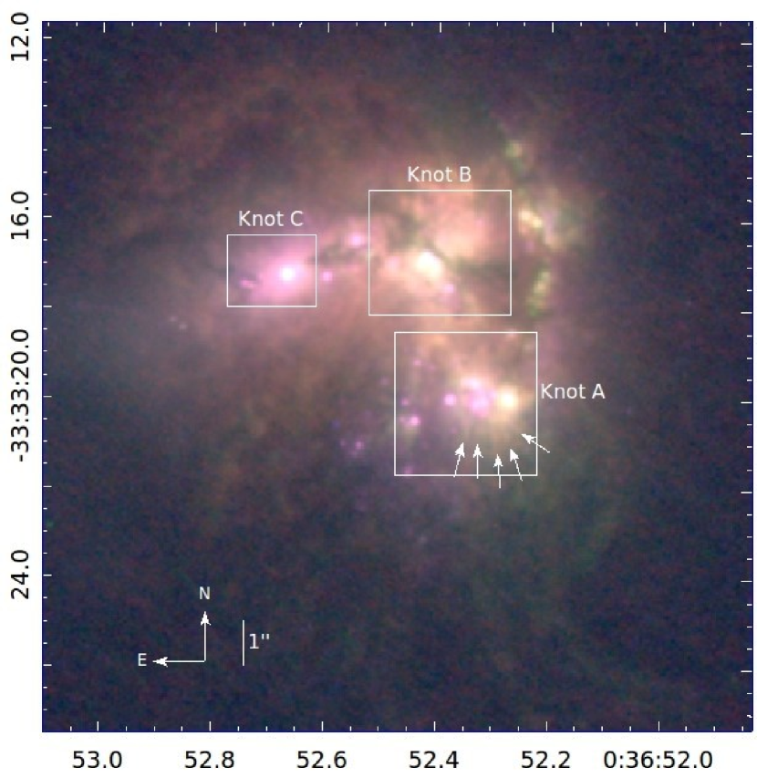
Figure 1: Three-color image of Haro 11 in [Oii] (WFC3/FQ378N), [Oiii] (ACS/F505N), and $U$ (ACS/F336W), corresponding to red, green, and blue, respectively. The three major star forming knots are labeled. White boxes correspond to subregions for each Knot used in calculating the scaling factor. The arrows indicate finger-like structures projecting from Knot A, suggesting a Giuliani instability. The scale bar shows $1\arcsec$, corresponding to 0.384 kpc.

Knot C has generally been considered the strongest candidate LCE since it is a strong Ly$\alpha$ source (Kunth et al., 2003; Östlin et al., 2009; Hayes, 2015). It is usually assumed that LCEs are also strong Ly$\alpha$ emitters since both phenomena require low Hi column densities. Knot B hosts an extremely bright ultraluminous X-ray source (ULX) dubbed Haro 11 X-1 by Prestwich et al. (2015). They suggest that this source could be a low luminosity AGN (LLAGN), which is especially interesting given results suggesting that faint AGN could produce sufficient energy to explain cosmic reionization (e.g., Madau & Haardt, 2015; Giallongo et al., 2015). However, there is no significant Ly$\alpha$ detection from Knot B (Östlin et al., 2009; Hayes, 2015).

Identifying which of the Knots is the LyC source in Haro 11 is therefore essential to understanding the conditions responsible for LyC escape. Can we confirm the expected correlation between LyC escape and Ly$\alpha$ escape, which would implicate Knot C? Is the possible LLAGN in Knot B responsible, implying that the dominant Ly$\alpha$ source is essentially unrelated to the LyC source? Or could the LyC emission originate from an entirely different location, in particular, Knot A? Since we cannot presently obtain spatially resolved imaging of LyC in Haro 11, we apply the technique of ionization-parameter mapping (IPM; Pellegrini et al., 2012) to better understand the nebular ionization structure of Haro 11 and locate its source of LyC leakage.

2 Ionization-Parameter Mapping of Haro 11

IPM entails constructing nebular emission-line ratio maps using two ions with high and low ionization potentials, for example, [Oiii]/[Sii]. The boundary of optically thick regions can be identified by a layer of emission in the low-ionization species, whereas optically thin regions show emission only in the unbounded, high-ionization species. By locating the most optically thin regions, IPM can provide indirect evidence for the presence of LyC escape features. We caution that optically thick boundary regions with low surface brightness can sometimes be difficult to detect, but IPM provides quick insight for identifying areas that are strong candidates for LyC escape. Our group has successfully used this method to identify candidate optically thin Hii regions in the Magellanic Clouds (Pellegrini et al., 2012), as well as such features in local starburst galaxies (Zastrow et al., 2011, 2013). Here, we apply IPM to Haro 11, using the [Oiii]$\lambda$5007 line as our high-ionization species and [Oii]$\lambda$3727 as our low-ionization species. The choice of line pairs from the same element controls for any element abundance variations across the galaxy.

We used the Hubble Space Telescope (HST) to obtain narrowband imaging, using both the WFC3 and ACS cameras. To obtain the [Oii]$\lambda$3727 imaging, we used WFC3 with the FQ378N filter, and for [Oiii]$\lambda$5007, we used the ACS FR505N ramp filter centered at 5110Å to account for Haro 11’s redshift of $z\sim 0.021$ (Bergvall et al., 2000). The [Oii] continuum image was obtained using the WFC3 F336W filter. For [Oiii] continuum an archival image in the ACS F550M filter was used. In addition, we used archival imaging of Haro 11 H$\alpha$ emission in the FR656N ramp filter, centered at 6698Å. We obtained a continuum image to pair with H$\alpha$ using the WFC3 F763M filter. Total exposure times for WFC3 images were 8416 s in FQ378N, 1332 s in F336W, and 627 s in F763M; exposure times for ACS were 2379 s in FR505N, 471 s in F550M, and 680 s in FR656N.

The STScI data pipeline provides flux-calibrated science images. Due to the sparseness of stars in our images, we used star clusters within the galaxy to align the images. These sources are unresolved and behave like point sources in our images. We required that the centroids of point sources be within 0.3 pixels of one another in every image, and a closer match was usually obtained for each narrowband image and its continuum counterpart.

2.1 A New Approach to Continuum Subtraction: Mode of the flux distribution

The narrowband images represent the sum of the line and continuum emission, with the latter due primarily to diffuse stellar background light. Ordinarily, the continuum emission is removed by subtracting an off-line image containing only continuum emission. This continuum image needs to be scaled by a scale factor $\mu$ to allow for differences in filter band width, and more importantly, the variation of the continuum spectral energy distribution (SED) between the two filters. Optimal scaling of the continuum filter flux is difficult to determine and complicated by spatial variations in the stellar background population, which have correspondingly varying SEDs. However, this issue is important for IPM, since improper continuum subtraction in one or both emission-line images can significantly affect the line ratios calculated and the features that appear in ionization-parameter maps.

Common methods for finding the scale factor $\mu$ include (1) using the relative intensity of line-free objects or regions in the image, and (2) taking the ratio of transmission efficiency for the filters. Hayes et al. (2009) and James et al. (2016) use spatially resolved approaches in which (3) the background SED is fitted for each image pixel, or binned pixels. The complications of these and other methods are reviewed by Hayes et al. (2009) and Hong et al. (2014). Haro 11 is in a relatively sparse field and our images did not contain enough sources outside the galaxy to apply approach (1). Approach (2) does not account for the continuum SED and produced bad oversubtraction in parts of our images. Method (3) is heavily model-dependent and complicated to implement. We therefore seek a relatively simple, empirically based method to apply to Haro 11. Hong et al. (2014) describe a promising method for determining the scaling factor using the skewness of the pixel histogram of the continuum subtracted image as a function of $\mu$. They find this relation to be sensitive to the ratio of line to continuum emission in the line image. In particular, when the line-to-continuum ratio is high, the optimal scaling is not well constrained by the skew. Since we are especially interested in regions at large galactocentric radius which are dominated by such conditions, this motivates us to investigate other, similar statistical methods for determining the best scaling. The use of a statistical measure on a large region of the image more directly addresses the goal of maximizing the number of pixels for which a given $\mu$ is optimized.

The optimal continuum scale factor must be that which neutralizes background continuum flux. We experimented with using the standard deviation $\sigma$, median, and mode of the continuum-subtracted pixel values, in a spirit similar to Hong’s et al. use of the skew. The standard deviation is that from the mean:

$$\sigma^{2}=\frac{\sum_{n=1}^{N}(x_{n}-X)^{2}}{N-1}\quad,$$ (1)

where $\sigma$ is the standard deviation, $N$ is the total number of pixels, $x_{n}$ is the flux in the $n$th pixel, and $X$ is the mean. To calculate the median and mode, a histogram is created by binning the pixels into bins of 0.5$\sigma$, which we found created large enough bins to accurately determine the mode across the image without washing out variations introduced by different values of $\mu$. We used IRAF routines to find the median and mode. The median is found by integrating the histogram, and using interpolation to find the value at which exactly half of the pixels are below and half above. The mode is found by locating the maximum of the histogram, then fitting a peak by parabolic interpolation. In the event that the first or last bin of the histogram is the maximum value, then that bin is assigned as the mode.

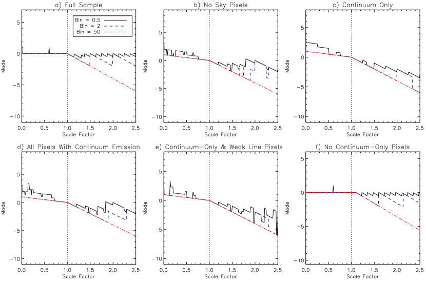
Figure 2: The behavior of mode vs. $\mu$ for the fiducial synthetic dataset. The dashed vertical line shows the true scale factor of 1. Bin sizes of 0.5, 2, and 50 are shown by solid black, dashed blue, and dot-dashed red lines, respectively. Each panel shows a different combination of pixels: (a) the full fiducial dataset, consisting of “sky” pixels with zero emission, continuum-only pixels, line-only pixels, and pixels with line-to-continuum ratios ranging from 0.1-10; (b) the fiducial dataset, excluding sky pixels; (c) only pixels with pure continuum emission; (d) continuum-only pixels and pixels with line-to-continuum ratios ranging from 0.1-10; (e) continuum-only pixels and pixels with a line-to-continuum ratio of 0.1; (f) the fiducial dataset, excluding the continuum-only pixels.

We find that the mode of the image pixel values has the most promising behavior. The mode should decrease smoothly as the continuum is subtracted; once the continuum becomes oversubtracted, negative pixels will cause rebinning of the pixel histogram, inducing a change in the relation. To explore the behavior of the mode with scale factor $\mu$, we generate an artificial dataset consisting of background pixels with no emission, and pixels with varying ratios of line and continuum emission. For our fiducial model, we consider six categories containing four pixels each: (i) background pixels with 0 counts each, (ii) continuum-only pixels with continuum fluxes of 1-4 counts, (iii) diffuse line-emitting pixels with line fluxes of 1-4 counts and no continuum emission, (iv) pixels with continuum fluxes of 1-4 counts and a line-to-continuum ratio of 0.1, (v) pixels with continuum fluxes of 1-4 counts and a line-to-continuum ratio of 1, and (vi) pixels with continuum fluxes of 1-4 counts and a line-to-continuum ratio of 10. We then vary the distribution of counts within each category, the relative numbers of pixels in each category, the background level in all pixels, and the bin size used to calculate the mode. We show different combinations of these pixel categories and bin sizes in Figure 2 and summarize the relevant results below.

The optimal scale factor represents the point when the emission of the continuum-only pixels exactly cancels out, reaching the background level. These pixels start out with some initial distribution of flux values. As $\mu$ is increased, their average flux and mode value decrease. At the optimal scale factor, their flux values pile up at the background level and then spread out again toward a range of negative values as the pixels become increasingly over-subtracted. Notably, the pixels that start out with the strongest continuum fluxes show the most rapid decrease in flux with scale factor. These pixels have the highest flux values before the optimal scale factor and the most negative values after the optimal scale factor. Since flux bins are defined starting with the lowest data values, the pixels with the weakest continuum flux set the mode bin value just below the transition point $\mu$ value, while the pixels with the strongest continuum flux set the mode bin value above the transition. This transition therefore corresponds to a change in slope in a plot of mode vs. $\mu$, as seen in Figure 2.

The mode-based continuum subtraction method works best when the image contains a large number of pixels with pure continuum emission (Figure 2a–e). However, in cases where background pixels dominate the mode value, this method is sensitive to even a single over-subtracted pixel. Once a pixel’s flux decreases below the background level, it defines the value of the lowest flux bin; since all other flux bins are defined as integer numbers of bins after the first bin, the lowest bin sets the lower and upper flux limits of all subsequent bins. The first over-subtracted pixel can therefore redefine the value of the bin that contains the background pixels and change the mode value. Pixels containing both line and continuum emission behave similarly to the pure continuum pixels but reach their over-subtraction point at higher scale factor values (Figure 2f). If no pure continuum pixels are present, the pixels with line emission will generate the observed slope transition and the true scale factor will be overestimated; the observed transition point therefore sets an upper limit on the optimal scale factor. The mode values for diffuse-line and background pixels do not depend on the scale factor, because they have no continuum emission. When present, these continuum-free pixels can set the initial mode value (e.g., Figure 2a,f), but the exact bin that contains this mode value will vary depending on the value of the lowest flux bin. We again emphasize that the mode-based method is sensitive to the first over-subtracted pixels, including ones with spuriously low values. However, the optimal value should still induce a subsequent transition as well. This method therefore requires empirical verification of the best value for $\mu$.

Because the slope transition represents a change in the value of the lowest flux bin, it occurs at the same scale factor regardless of the bin size used to calculate the mode; however, the change is most obvious with large bin sizes (Figure 2). Small bin sizes may show more discontinuities, as pixels abruptly shift into or out of a bin. Nevertheless, the overall slope on either side of the discontinuity remains constant and only changes at the optimal scale factor. Oscillations typically appear after the optimal scale factor, and their amplitude and frequency depend on bin size. As over-subtracted pixels decrease in flux, they continually re-define the value of the lowest flux bin and all higher flux bins. The value of the flux bin that contains the mode will oscillate as the mode changes from the highest value in its flux bin to the lowest value in its flux bin. Larger bin sizes wash out discontinuities and oscillations, so that the only remaining transition is the slope change as over-subtraction begins.

Figure 3 shows the mode as a function of scale factor for our imaging in each line. For the whole-frame images (black), we find clear breaks in this relation for each line, which give scaling values of $\mu_{\rm WF}=0.127$ for [Oii], $\mu_{\rm WF}=0.179$ for [Oiii], and $\mu_{\rm WF}=0.395$ for H$\alpha$. Figure 4 shows, as an example, the H$\alpha$ image, continuum-subtracted using the mode method. Here, we see an example where the second slope break, rather than the one at the lowest $\mu$, corresponds to the optimal scale factor. We also determine the scale factors for smaller regions around each Knot, shown in Figure 3, with Knot A in cyan, Knot B in red, and Knot C in blue. The regions are shown by the white boxes in Figure 1. For Knot A, we find a good fit in all bands, which generally agrees well with the scale factor for the entire image. We find $\mu_{A}=0.127$ for [Oii], $\mu_{A}=0.191$ for [Oiii], and $\mu_{A}=0.396$ for H$\alpha$. Determining the scale factor is most difficult in Knot B. For [Oii], there is no obvious point at which the slope changes, although around $\mu_{B}\sim 0.2$ would be an upper limit. For [Oiii] we find a clear optimal value at $\mu_{B}=0.266$. For H$\alpha$, we find no break below $\mu_{B}=0.500$. The break in the mode for Knot B occurs at a much higher value than for the other regions, in all bands. This implies that the continuum is fainter in this region, which may be related to the pronounced dust lane seen in Figure 1. For Knot C, we find $\mu_{C}=0.125$ for [Oii] and $\mu_{C}=0.445$ for H$\alpha$. For [Oiii], there is a clear break where noise begins at $\mu_{C}=0.191$, consistent with values for other regions. Comparison of the mode for the entire image, Knot A, Knot B, and Knot C shows that Knots A and C typically have very similar scaling, and agree with the scaling for the whole image.

Due to the close agreement between three of our four measurements, we chose to use the scale factor determined for the whole frame to calibrate our final [Oiii]/[Oii] ratio map, which is shown in the center panel of Figure 5. These values are $\mu_{\rm WF}=0.127\pm 0.002$ for [Oii], $\mu_{\rm WF}=0.179\pm 0.012$ for [Oiii], and $\mu_{\rm WF}=0.395\pm 0.050$ for H$\alpha$, where the errors are determined by the maximal difference between the scale factor for the full frame, Knots A and C. These values produce images with few or no continuum pixels subtracted below the level of the background, and with greatly decreased continuum flux compared to unsubtracted images. Using a single scale factor for the whole galaxy ignores spatial variations in the continuum SED, and Figure 3 shows that some variation is present, as expected. However, since we are mainly interested in the [Oiii]/[Oii] ratio map at large galactocentric distances, this ratio is fairly insensitive to the exact value of $\mu$, since the continuum has very low emission, if any, in these regions.

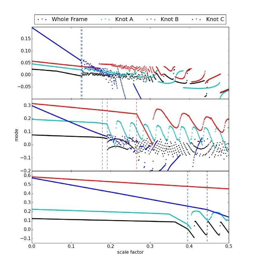
Figure 3: Mode of continuum-subtracted pixel values as a function of scale factor $\mu$ for [Oii] (top), [Oiii] (middle) and H$\alpha$ (bottom). The whole frame and subregions defined in Figure 1 are distinguished with the shown colors. The vertical dashed lines show the adopted $\mu$ values, using the same color scheme.

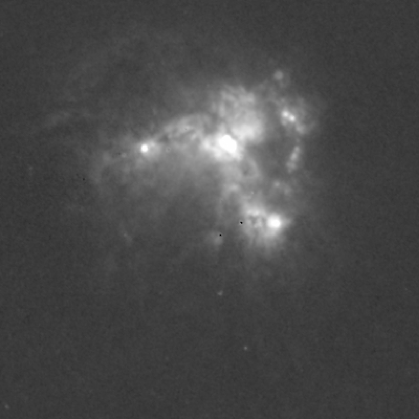
Figure 4: Continuum-subtracted, emission-line image in H$\alpha$.

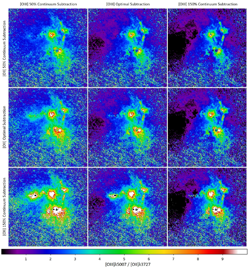
Figure 5: Ratio maps of [Oiii]/[Oii] for different combinations of errors in continuum subtraction. Maps in the left, center, and right columns are constructed with [Oiii] continuum subtraction of $0.5\times\mu_{\rm WF}$, $1.0\times\mu_{\rm WF}$, and $1.5\mu_{\rm WF}$, respectively. The upper and lower rows have [Oii] continuum subtraction at $0.5\times\mu_{\rm WF}$, $1.0\times\mu_{\rm WF}$, and $1.5\times\mu_{\rm WF}$, respectively. The center panel shows the ratio map created using the optimal continuum subtraction in both bands.

3 LyC Source Candidates

3.1 Ionization Parameter Mapping

The center panel of Figure 5 shows the optimally continuum-subtracted ratio map of [Oiii]/[Oii] emission. There is a highly ionized region extending at least 3$\arcsec$ ($>1$ kpc) from the center of Knot A into the outskirts of the galaxy to the south and southwest. The lack of a clear transition to low [Oiii]/[Oii] at the edge of this region strongly suggests that it is optically thin and may be allowing the escape of LyC into the circumgalactic medium. By contrast, the confined morphology of [Oiii]/[Oii] for the rest of the galaxy, in particular, around Knots B and C, suggests that these other regions are surrounded by optically thick envelopes. The detection of this highly ionized region extending from Knot A is robust to errors in continuum subtraction. Figure 5 shows the ratio maps constructed from [Oiii] images with the continuum subtracted at $0.5\times\mu_{WF}$ (left column), $1.0\times\mu_{WF}$ (center column), and $1.5\times\mu_{WF}$ (right column), and [Oii] images subtracted at the same increments in the top, center, and bottom rows, respectively. Thus, the ratio map with optimal subtraction in both images appears in the center panel. We note that our analysis of the continuum scaling above (§ 2.1) suggests an uncertainty in $\mu$ of less than a factor of 0.1 for both [Oii] and [Oiii]. The extended, high-ionization region is present in all cases, despite notable changes in the appearance of other regions. It is especially noteworthy that Knot C, which is usually assumed to be the LyC-emitting region, generally appears to be optically thick in the LyC, although it is optically thin in Ly$\alpha$ (Kunth et al., 2003). Knot C does show an ionized region stretching to the east in the case where we undersubtract the continuum in [Oiii] and oversubtract in [Oii] (Figure 5, lower left quadrant). However, this feature only appears when very large errors in continuum subtraction are assumed.

IPM in [Oiii]/[Oii] primarily maps the galaxy’s ionization structure in the plane of the sky. However, assuming the LyC detection from Haro 11 is real, we should also expect at least one ionized region to be optically thin to LyC along the line of sight, to explain previous direct detections of LyC emission from Haro 11. The ratios of [Oii] and [Oiii] to H$\alpha$ can be used as an indicator for ionization in the line of sight (Pellegrini et al., 2012). In particular, a region is likely to be optically thin when it shows both a high [Oiii]/H$\alpha$ ratio and low [Oii]/H$\alpha$ $\lesssim 0.1$. Weak [Oii]/H$\alpha$ again indicates the lack of a nebular zone in the low ionization species, whereas a comparatively high [Oiii]/H$\alpha$ ratio in the same line of sight then indicates that the gas is highly ionized. Figure 6 shows maps of these ratios. Knot A indeed has both low [Oii]/H$\alpha$ and high [Oiii]/H$\alpha$, indicating it is likely optically thin in the line of sight. This further indicates that Knot A is a strong candidate for the galaxy’s LyC emission source. Knot B also shows extremely low values of [Oii]/H$\alpha$, but the excitation is much lower in Knot B, as indicated by lower [Oiii]/H$\alpha$. Furthermore, as we have seen above, the continuum subtraction for [Oii] in Knot B is uncertain. Dust could play a role in suppressing the [Oii] line emission relative to the redder [Oiii] line. There is a noticeable dust lane through the region, which adds further uncertainty to any conclusions about Knot B. We also see no indication that Knot C is optically thin in the line of sight.

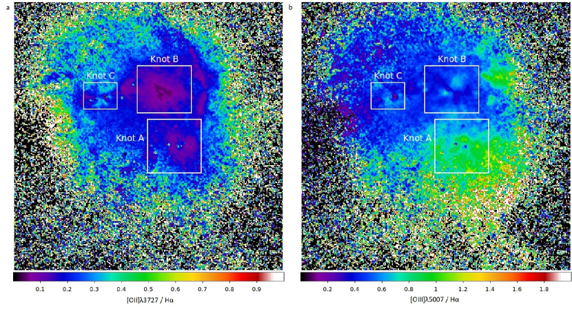
Figure 6: Panel a: [Oii]/H$\alpha$ ratio map. Panel b: [Oiii]/H$\alpha$ ratio map. The combination of strong [Oiii] and low [Oii] suggests Knot A as a source for direct detections of LyC from Haro 11. A small localization on Knot B is also a candidate.

3.2 A, B, or C? Implications for LyC Escape

Of the three dominant sources in Haro 11, both Knots B and C have previous evidence suggesting that they could be the LyC source(s). Knot C is visually the brightest knot and shows strong Ly$\alpha$ emission (Kunth et al., 2003; Östlin et al., 2009; Hayes, 2015). It appears to be the nucleus of one of the two galaxies in this merging system (James et al., 2013; Östlin et al., 2015), and Prestwich et al. (2015) also identify Knot C as the host of a ULX source with an X-ray luminosity of $L_{X}\sim 5\times 10^{40}$ erg s^-1, dubbed Haro 11 X-2. They suggest that this source may provide enough mechanical power to clear channels through the ISM promoting a low Ly$\alpha$ optical depth. Such geometry would also enhance the escape of LyC radiation. However no previous work has been able to directly attribute LyC emission to Knot C, and Rivera-Thorsen et al. (2017) find that the column density of neutral gas in the Knot is too high to allow LyC escape from a density bounded ISM, although they suggest it may be possible if the covering fraction of denser gas is less than unity. While we find that Knot C exhibits an ionization feature to the east in one calibration of the continuum subtraction (Figure 5), our optimal subtraction shows Knot C to be in a low ionization state compared to much of the galaxy, which does not support it being the LyC source.

In Knot B, Prestwich et al. (2015) report an unusually luminous ULX with $L_{X}\sim 10^{41}$ ergs s^-1, which could be a low-luminosity AGN. Recent models have suggested that LLAGN could be important, or even vital, for cosmic reionization (Fontanot, Cristiani, & Vanzella, 2012; Madau & Haardt, 2015; Giallongo et al., 2015). It should also be noted that LLAGN are now known to be relatively common in dwarf galaxies (e.g., Reines et al., 2013; Lemons et al., 2015; Baldassare et al., 2015). However, Prestwich et al. (2015) note that the source in Knot B is more likely to be a luminous X-ray binary, and possibly a supermassive black hole progenitor. They show that an X-ray binary could produce mechanical power comparable to the supernova feedback for an entire cluster, indicating that such a system could clear paths for LyC escape. Thus, Haro 11 may provide an important opportunity to evaluate AGN, or possibly black hole binaries, versus massive stars as cosmic LyC sources. Figure 6 shows that Knot B itself exhibits a low ratio of [Oii]/H$\alpha$ suggesting that it may be a LyC leakage source along the line of sight. However, it is clearly ionization-bounded transverse to our sightline in our [Oiii]/[Oii] ratio maps, showing no signs of LyC escape along the plane of the sky. Thus if Knot B is optically thin, it would be consistent with suggestions that LyC leakage is not isotropic, but would require an especially narrow ionization cone along the line of sight to show no hints in other directions (e.g., Zastrow et al., 2011). Our data cannot definitively rule out Knot B as the dominant LyC emitter in Haro 11.

In contrast to the negative and ambiguous results for Knots C and B, respectively, our ionization-parameter mapping indicates that Knot A may be the strongest candidate for the LyC emission. The large, highly ionized region extending to the outskirts of the galaxy implies that the region southwest of Knot A is optically thin to LyC and could allow large escape fractions in those directions. Preliminary results presented by Bik et al. (2015) for [Sii]/[Oiii] ratios also show this feature. In addition, the low ratio of [Oii]/H$\alpha$ for Knot A itself suggests that this potentially optically thin region also extends along our line of sight. We have no reason to expect that large dust clouds could systemically depress the [Oii] relative to [Oiii] flux in the galaxy outskirts. Additionally the observations by Bik et al. (2015) use tracers where the high ionization species is the bluer line, ruling out reddening as an explanation. Thus, we consider Knot A to be at least as good a candidate for the origin of LyC emission as Knots B and C, and likely even stronger.

Previous studies have found LyC-leaking candidates with narrow, cone-shaped LyC escape regions (Zastrow et al., 2013, 2011). The ionization in Knot A is over a broader region than the cones reported in other galaxies, but still covers only a limited directional range, adding further support to suggestions that LyC escape is highly nonuniform across regions of a galaxy. The growing number of galaxies with relatively narrow ionization regions suggests that line of sight bias is a problem for direct searches for galaxies with high LyC escape fractions.

Knot A also exhibits other noteworthy features. In particular, Figures 1 and 3 show remarkable, finger-like structures projecting southwards from the knot. These structures are startlingly similar to those seen in simulations by Freyer et al. (2003) and García-Segura & Franco (1996). The dominant effect is the Giuliani (1979) instability, which is a specific case of the Vishniac (1983) thin shell instability applied to ionization fronts. The simulations show that ionized fingers form at extremely early stages in Hii region evolution, on the order of $10^{5}$ yr. They occur when the instability causes the thin shell driven by the ionization front to fragment, leading to recombination in the remnant clumps, which cast shadows between the low-density, ionized fingers. The effect can be amplified by mechanical feedback from a wind-driven shell (Freyer et al., 2003). On a similar timescale, the clumps then merge into a more amorphous configuration and are swept up by the stellar wind shell, causing the fingers to disappear again. Thus, these ionized features are short-lived phenomenon that appear at a very early stage of the massive star feedback.

The features in Knot A appear to be examples of the Giuliani instability. The morphology of the fingers is uniform and consistent with light rays emitted through shadowed regions, as opposed to showing irregular surfaces of dense gas, as seen in pillars. This is consistent with the radiation-dominated conditions indicated by the extreme ionization seen in Figures 5 – 6, and probable optically thin state, in the same directions. Finally, these directions lead directly out from the galaxy into a lower density environment, which is again a condition promoting the Giuliani effect. Interestingly, the extremely young age, $\lesssim 1$ Myr, is also implied in the nearby LyC candidate Mrk 71 (Micheva et al., 2017). The extreme Green Pea galaxies, which are the best class of local LCE candidates, also have young ages, in some cases $\lesssim 2$ Myr (Jaskot & Oey, 2013).

The suggestion of such an extremely young age for Knot A is at odds with the slightly more evolved age of 4.9 Myr reported by James et al. (2013). This value is driven by the presence of WR stars within the stellar population synthesis models; since WR stars form around 3 – 5 Myr, the models yield corresponding instantaneous burst ages when WR features are detected. However, recent work is pointing to the contribution of very massive stars (VMS) with masses $>100\ \rm M_{\odot}$ to WN features in the extremely young super star clusters 30 Doradus in the LMC (Crowther et al., 2010, 2016) and NGC 5253-5 (Smith et al., 2016). The latter work shows that strong VMS candidates in NGC 5253-5 generate only broad, He ii $\lambda 4686$ emission, with no stellar [N iii] $\lambda\lambda 4634-4641$ contribution to the WR blue bump. We note that the same is observed in Knots A and B of Haro 11, as seen in the FLAMES IFU spectra of James et al. (2013, their Figure 10). NGC 5253-5 has an estimated age of $1\pm 1$ Myr (Calzetti et al., 2015), and 30 Dor similarly has an age of $1.5^{+0.3}_{-0.7}$ Myr (Crowther et al., 2016). Both systems are believed to be optically thin in the LyC (Zastrow et al., 2013; Pellegrini et al., 2012). Thus Knot A may be similar to these newborn, optically thin, super star cluster systems.

If Knot A, rather than Knot C, turns out to be the dominant LyC source in Haro 11, then this has major implications in understanding the relationship between Ly$\alpha$ and LyC emission. In general, it is assumed that LyC emitters are also Ly$\alpha$ emitters, since Ly$\alpha$ is produced by the recombination of ionizing radiation, and the optical depth of Ly$\alpha$ is extremely sensitive to small Hi columns. Thus, the conditions for Ly$\alpha$ escape are also similar to those of LyC escape. However, we note that the escape processes differ substantially: Ly$\alpha$ is optically thick at an Hi column $\log N$(Hi)$\sim 13$ that is $10^{4}$ times lower than the threshold for LyC, $\log N$(Hi)$\sim 17$. Thus, in many situations, regions that are optically thin in LyC will be optically thick to Ly$\alpha$. However, Ly$\alpha$ scatters strongly and may re-emitted non-isotropically and far from the original line of sight. Much longer path lengths also enhance dust absorption of Ly$\alpha$ relative to LyC. Thus, the relationship between these two escape processes may be more complicated than is generally appreciated. For Haro 11, we find that, while this galaxy emits in both LyC and Ly$\alpha$, the respective sources may not coincide. Spatially resolving the LyC emission in this galaxy will greatly clarify our understanding of the radiative transfer.

4 Conclusions

In summary, we use HST WFC3 and ACS narrow-band imaging to carry out ionization-parameter mapping in an attempt to clarify the spatial origin of the LyC emission in Haro 11. We present a new statistical method for optimizing the continuum subtraction, based on the mode of the image flux distribution. Applying this technique, we obtain continuum-subtracted, emission-line images in [Oiii], [Oii], and H$\alpha$, providing spatially resolved insight on the LyC escape in this known LyC-emitting galaxy. Haro 11 has strong Ly$\alpha$ emission from Knot C and may host a LLAGN in Knot B, which are both potential indicators of a LyC source. However, we find no evidence for LyC escape from Knot C, consistent with recent results of Rivera-Thorsen et al. (2017). Knot B is likely optically thin to LyC along the line of sight, as indicated by a low [Oii]/H$\alpha$ ratio on the center of the Knot. However, along the plane of the sky, Knot B shows a smooth drop in [Oiii]/[Oii], indicating that it is radiation-bounded.

Instead, we find the strongest evidence for LyC escape to be from Knot A, which has not previously been suggested as a candidate for the LyC source. The [Oiii]/[Oii] ratio maps show a highly ionized region extending at least 1 kpc from the center of the Knot into the surrounding medium, suggesting that it is optically thin to LyC radiation. Additionally a low [Oii]/H$\alpha$ ratio at the center of Knot A implies that it is also optically thin along the line of sight, further enhancing the possibility that it is the source of directly detected LyC radiation. We suggest that the observed broad He ii $\lambda 4686$ emission in Knot A may be due to VMS stars rather than classical WR stars, pointing to an extremely young age on the order of 1 Myr. This is consistent with the appearance of ionized fingers that may be generated by the Giuliani instability. It is possible that the candidate knots each provide partial contributions to the LyC emission, which suggests the possibility that a combination of LLAGN/accretion and stellar feedback may generate LyC leakage. If Knot A is confirmed as the LyC source, this result would have strong implications for our understanding of the relationship between Ly$\alpha$ and LyC emission, implying that although Knot C is a strong Ly$\alpha$ emitter, it may be an insignificant LyC emitter, while the opposite may be the case in Knot A. This would imply that Ly$\alpha$ and LyC emission might be substantially independent. It would also provide further evidence that LyC escape is highly anisotropic and therefore challenging to detect directly (e.g., Zastrow et al., 2011). Further work is needed to identify which of the Knots is the true source of the observed LyC radiation in Haro 11: the candidate presented in this work via IPM, Knot A; the ULX and possible LLAGN, Knot B; or the strong Ly$\alpha$ source, Knot C.

References

- Adamo et al. (2010) Adamo, A., Östlin, G., Zackrisson, E., et al. 2010, MNRAS, 407, 870
- Baldassare et al. (2015) Baldassare, V. F., Reines, A. E., Gallo, E., & Greene, J. E. 2015, ApJL, 809, L14
- Bergvall et al. (2000) Bergvall, N. Masegosa, J., Östlin, G., & Cernicharo, J., A&A, 359, 41B
- Bergvall & Östlin (2002) Bergvall, N. & Östlin, G. 2002, A&A, 390, 891
- Bergvall et al. (2006) Bergvall, N., Zackrisson, E., Andersson, B.-G., et al. 2006 A&A, 448, 513
- Bik et al. (2015) Bik, A., Östlin, G., Menacho, V., Adamo, A., Hayes, M., et al. 2015, Proceedings IAU Symposium No. 316
- Calzetti et al. (2015) Calzetti, D., Johnson, K. E., Adamo, A., et al. 2015, ApJ 811, 75
- Clarke & Oey (2002) Clarke, C. J. & Oey, M. S., 2002, MNRAS, 337, 1299
- Crowther et al. (2010) Crowther, P. A., Schnurr, O., Hirschi, R., Yusof, N., Parker, R. J., Goodwin, S. P., & Kassim, H. A. 2010, MNRAS 408, 731
- Crowther et al. (2016) Crowther, P. A., Caballero-Nieves, S. M., Bostroem, K. A., et al. 2016, MNRAS 458, 624
- Fontanot, Cristiani, & Vanzella (2012) Fontanot, F., Cristiani, S., & Vanzella, E. 2012, MNRAS, 425, 1413
- Fontanot et al. (2014) Fontanot, F., Cristiani, S., Pfrommer, C., Cupani, G., & Vanzella, E. 2014, MNRAS 438, 2097
- Freyer et al. (2003) Freyer, T., Hensler, G., & Yorke, H. W., 2003, ApJ, 594, 888
- Fujita et al. (2003) Fujita, A., Martin, C. L., Mac Low, M.-M., & Abel, T. 2003, ApJ 599, 50
- García-Segura & Franco (1996) García-Segura, G., & Franco, J. 1996, ApJ, 469, 171
- Giallongo et al. (2015) Giallongo, E., Grazian, A., Fiore, F., et al. 2015, A&A, 578, A83
- Giuliani (1979) Giulianin, J. L. 1979, ApJ, 233, 280
- Hayes et al. (2009) Hayes, M., Östlin, G., Mas-Hesse, J. M., & Kunth, D., 2009, AJ, 138, 911
- Hayes (2015) Hayes, M., 2015, PASA, 32, e027
- Hong et al. (2014) Hong, S., Calzetti, D., & Dickinson, M. 2014, PASP, 126, 79
- Izotov et al. (2016a) Izotov, Y. I., Orlitová, I., Schaerer, D., et al. Nature, 529, 178
- Izotov et al. (2016b) Izotov, Y. I., Schaerer, D., Thuan, T. X., et al. 2016, MNRAS, 461, 3683
- James et al. (2013) James, B. L., Tsamis, Y. G., Walsh, J. R., Barlow, M. J., & Westmoquette, M. S. 2013, MNRAS, 430, 20974
- James et al. (2016) James, B. L., Auger, M., Aloisi, A., Calzetti, D., & Kewley, L. 2016, ApJ, 816, 40
- Jaskot & Oey (2013) Jaskot, A. E., & Oey, M. S., 2013, ApJ, 766, 91
- Kunth et al. (2003) Kunth, D., Leitherer, C., Mas-Hesse, J. M., Östlin, G., & Petrosian, A. 2003, ApJ, 597, 263
- Leitet et al. (2011) Leitet, E., Bergvall, N., Piskunov, N., & Andersson, B.-G. 2011, A&A, 532, A107
- Leitet et al. (2013) Leitet, E., Bergvall, N., Hayes, M., Linné, S., & Zackrisson, E. 2013, A&A, 553, A106
- Lemons et al. (2015) Lemons, S. M., Reines, A. E., Plotkin, R. M., Gallo, E., & Greene, J. E. 2015, ApJ, 805, 12
- Madau & Haardt (2015) Madau, P., & Haardt, F. 2015, ApJL, 813, L8
- Micheva et al. (2017) Micheva, G., Oey, M. S., Jaskokt, A. E., & James, B. L. 2017, ApJ, in press; astro-ph/1704.01678
- Östlin et al. (2001) Östlin, G., Amram, P., Bergvall, N., et al. 2001, A&A, 374, 800
- Östlin et al. (2009) Östlin, G., Hayes, M., Kunth, D., et al. 2009, AJ, 138, 923
- Östlin et al. (2015) Östlin, G., Marquart, T., Cumming, R. J., et al. 2015, A&A, 585, A55
- Pellegrini et al. (2012) Pellegrini, E. W., Oey, M. S., Winkler, P. F., et al. 2012, ApJ, 755, 40
- Prestwich et al. (2015) Prestwich, A. H., Jackson, F., Kaaret, P., et al. 2015, ApJ, 812, 166
- Reines et al. (2013) Reines, A. E., Greene, J. E., & Geha, M. 2013, ApJ, 775, 116
- Rivera-Thorsen et al. (2017) Rivera-Thorsen, T. E., Östlin, G., Hayes, M., & Puschnig, J. 2017, ApJ 837, 29
- Rutkowski et al. (2016) Rutkowski, M. J., Scarlata, C., Haardt, F., et al. 2016, ApJ, 819, 81
- Siana et al. (2015) Siana, B., Shapley, A. E., Kulas, K. R., et al. 2015, ApJ, 804, 17
- Smith et al. (2016) Smith, L. J., Crowther, P. A., Calzetti, D., & Sidoli, F. 2016, ApJ, 823, 38
- Vader et al. (1993) Vader, J. P., Frogel, J. A., Terndrup, D. M., & Heisler, C. A. 1993, AJ, 106, 1743
- Verhamme et al. (2015) Verhamme, A., Orlitová, I., Schaerer, D., & Hayes, M. 2015, A&A, 578, A7
- Vishniac (1983) Vishniac, E. T. 1983, ApJ, 274, 152
- Zastrow et al. (2011) Zastrow, J., Oey, M. S., Veilleux, S., McDonald, M., & Martin, C. L. 2011, ApJL, 741, L17
- Zastrow et al. (2013) Zastrow, J., Oey, M. S., Veilleux, S., & McDonald, M. 2013, ApJ, 779, 76