Adequacy of the Gradient-Descent Method for
Classifier Evasion Attacks

Abstract.

Despite the wide use of machine learning in adversarial settings including computer security, recent studies have demonstrated vulnerabilities to evasion attacks—carefully crafted adversarial samples that closely resemble legitimate instances, but cause misclassification. In this paper, we examine the adequacy of the leading approach to generating adversarial samples—the gradient descent approach. In particular (1) we perform extensive experiments on three datasets, MNIST, USPS and Spambase, in order to analyse the effectiveness of the gradient-descent method against non-linear support vector machines, and conclude that carefully reduced kernel smoothness can significantly increase robustness to the attack; (2) we demonstrate that separated inter-class support vectors lead to more secure models, and propose a quantity similar to margin that can efficiently predict potential susceptibility to gradient-descent attacks, before the attack is launched; and (3) we design a new adversarial sample construction algorithm based on optimising the multiplicative ratio of class decision functions.

1. Introduction

Recent years have witnessed several demonstrations of machine learning vulnerabilities in adversarial settings (Dalvi et al., 2004; Lowd and Meek, 2005; Barreno et al., 2006; Rubinstein et al., 2009; Brückner and Scheffer, 2011; Biggio et al., 2012; Goodfellow et al., 2014; Alfeld et al., 2016; Li et al., 2016). For example, it has been shown that a wide rage of machine learning models—including deep neural networks (DNNs), support vector machines (SVMs), logistic regression, decision trees and $k$-nearest neighbours ($k$NNs)—can be easily fooled by evasion attacks via adversarial samples (Biggio et al., 2013; Goodfellow et al., 2014; Moosavi-Dezfooli et al., 2016b; Nguyen et al., 2015; Papernot et al., 2016a; Papernot et al., 2016c).

We refer to the carefully crafted inputs that resemble legitimate instances but cause misclassification, as adversarial samples, and the malicious behaviours that generate them as evasion attacks (Russu et al., 2016). Figure 1 illustrates the attack’s effect in the previously-explored vision domain (Szegedy et al., 2013; Goodfellow et al., 2014; Papernot et al., 2016c): Figures 1(a) and 1(b) present original images from (Samaria and Harter, 1994) for “Adam” and “Lucas”, who are correctly identified by an SVM face recogniser. However, after human-indiscernible changes are applied to Figure 1(a) the model mistakenly identifies Figure 1(c) as “Lucas”.

(a) Adam

(b) Lucas

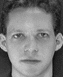
(c) Adam or Lucas?

Figure 1. An example evasion attack against a learning model: Image (c) is misclassified as Lucas.

Thanks to its approximation of best-response and simplicity, gradient descent has emerged as the leading approach for creating adversarial samples (Biggio et al., 2013). While plentiful in the literature, analyses of evasion attacks tend to present only a handful of adversarial samples like Figure 1, or attack success rates for limited hyperparameters settings. Such results are useful proofs of concept, but fail to provide a systematic analysis of the competence of the gradient descent method and best response more generally. Does the method have any structural limitations? Can gradient descent based evasion attacks be reliably thwarted, without cost to learner accuracy? Are there effective attack alternatives? This paper addresses these questions, with a case study on the support vector machine with radial basis function kernel.

To the best of our knowledge, this is the first rigorous evaluation of the gradient descent method in classifier evasion settings. Not only do we demonstrate that appropriate choice of smoothness (RBF SVM kernel width) can significantly degrade attack success, but that we can even predict when attacks will be successful without ever launching them.

Main contributions: Specifically, our contributions include:

• An analysis of the kernel precision parameter’s impact on the success rate of evasion attacks, illustrating the existence of a phase transition, and concluding that carefully reduced kernel smoothness achieves robustness to gradient-descent attacks without sacrificing SVM accuracy;

• A novel geometric parameter related to margin, that strongly correlates with model vulnerability, providing a new avenue to predict (unseen) attack vulnerability; and

• A new approach for generating adversarial samples in multiclass scenarios, with results demonstrating higher effectiveness for evasion attacks than the gradient descent method.

The remainder of this paper is organised as follows: Section 2 overviews previous work on evasion attacks; Section 3 presents our research problem; we present a detailed example of how gradient-descent can fail in Section 4; Section 5 presents the gradient-quotient approach for constructing adversarial samples; experimental results are presented in Sections 6 and 7; and Section 8 concludes the paper.

2. Related Work

Barreno et al. (2006) categorise how an adversary can tamper with a classifier based on whether they have (partial) control over the training data: in causative attacks, the adversary can modify the training data to manipulate the learned model; in exploratory attacks, the attacker does not poison training, but carefully alters target test instances to flip classifications. See also (Barreno et al., 2010; Huang et al., 2011). This paper focuses on the targeted exploratory case, also known as evasion attacks (Biggio et al., 2013).

Generalising results on efficient evasion of linear classifiers via reverse engineering (Lowd and Meek, 2005), Nelson et al. (2012) consider families of convex-inducing classifiers, and propose query algorithms that require polynomially-many queries and achieve near-optimal modification cost. The generation of adversarial samples in their setting leverages membership queries only: the target classifier responds to probes with signed classifications only. Formulating evasion as optimisation of the target classifier’s continuous scores, Biggio et al. (2013, 2014) first used gradient descent to produce adversarial samples.

Szegedy et al. (2013) demonstrate changes imperceptible to humans that cause deep neural networks (DNNs) to misclassify images. Additionally, they offer a linear explanation of adversarial samples and design a “fast gradient sign method” for generating such samples (Goodfellow et al., 2014). In a similar vein, Nguyen et al. (2015) propose an approach for producing DNN-adversarial samples unrecognisable as such to humans.

Papernot et al. published a series of further works in this area: (1) introducing an algorithm that searches for minimal regions of inputs to perturb (Papernot et al., 2016c); (2) demonstrating effectiveness of attacking target models via surrogates—with over 80% of adversarial samples launched fooling the victim in one instance (Papernot et al., 2016b); (3) improved approaches for fitting surrogates, with further investigation of intra- and cross-technique transferability between DNNs, logistic regression, SVMs, decision trees and $k$-nearest neighbours (Papernot et al., 2016a).

Moosavi-Dezfooli et al. (2016a) propose algorithm DeepFool for generating adversarial samples against DNNs, which leads samples along trajectories orthogonal to the decision boundary. A similar approach against linear SVM is proposed in (Papernot et al., 2016a). Based on DeepFool, Moosavi-Dezfooli et al. (2016b) design a method for computing “universal perturbations” that fool multiple DNNs.

In terms of defending against evasion attacks, Szegedy et al. (2013); Goodfellow et al. (2014) propose injecting adversarial examples into training, in order to improve the generalization capabilities of DNNs. This approach resembles active learning. Papernot et al. (2016d) demonstrate using distillation strategy against saliency map attack. But it has been proven to be ineffective by (Carlini and Wagner, 2016). Gu and Rigazio (2015); Shaham et al. (2016); Zhao and Griffin (2016); Luo et al. (2016); Huang et al. (2016); Carlini and Wagner (2017); Miyato et al. (2016); Zheng et al. (2016) have designed various structural modifications for neural networks. In addition, Bhagoji et al. (2017); Zhang et al. (2016) propose defense methods based on dimensionality reduction via principal component analysis (PCA), and reduced feature sets, respectively. However, they contradict with (Li and Vorobeychik, 2014) which suggests that more features should be used when facing adversarial evasion.

Most relevant to this paper is the work by Russu et al. (2016), which analyses the robustness of SVMs against evasion attacks, including the selection of the regularisation term, kernel function, classification costs and kernel parameters. Our work delivers a much more detailed analysis of exactly how the kernel parameters impact vulnerability of RBF SVM, and explanations of why.

3. Preliminaries & Problem Statement

This section recalls evasion attacks, the gradient-descent method, the RBF SVM, and summarises the research problem addressed by this paper.

Evasion Attacks. For target classifier $f:\mathbb{R}^{d}\to\{-1,1\}$, the purpose of an evasion attack is to apply minimum change $\boldsymbol{\delta}$ to a target input $\boldsymbol{x}$, so that the perturbed point is misclassified, i.e., $\mathrm{sgn}(f(\boldsymbol{x}))\neq\mathrm{sgn}(f(\boldsymbol{x}+\boldsymbol{\delta}))$. The magnitude of adversarial perturbation $\boldsymbol{\delta}$ is commonly quantified in terms of $L_{1}$ distance, i.e., $\left\|\boldsymbol{\delta}\right\|_{1}=\sum_{i=1}^{d}|\delta_{i}|$. Formally, evasion attacks are framed as optimisation:

(1) $$\arg\min_{\boldsymbol{\delta}\in\mathbb{R}^{d}} \left\|\boldsymbol{\delta}\right\|_{1}$$

s.t. $$\mathrm{sgn}(f(\boldsymbol{x}))\neq\mathrm{sgn}(f(\boldsymbol{x}+\boldsymbol{\delta}))\enspace.$$

Note that we permit attackers that can modify all features of the input, arbitrarily, but that aim to minimise the magnitude of changes. Both binary and multiclass scenarios fall into the evasion problem as described; we consider both learning tasks in this paper. In multiclass settings, attacks intending to cause specific misclassification of the test sample are known as mimicry attacks.

Gradient-Descent Method. The gradient descent method has been widely used for generating adversarial samples for evasion attacks (Biggio et al., 2013; Goodfellow et al., 2014; Moosavi-Dezfooli et al., 2016a; Papernot et al., 2016c), when $f$ outputs confidence scores in $\mathbb{R}$ and classifications are obtained by thresholding at $\tau=0$. The approach applies gradient descent to $f$ directly, initialised at the target instance. Formally given target instance $\boldsymbol{x}_{0}\in\mathbb{R}^{d}$ evaluating $f(\boldsymbol{x}_{0})>\tau$,

$$\boldsymbol{x}_{t+1} = \boldsymbol{x}_{t}-\varepsilon_{t}\cdot\nabla_{\boldsymbol{x}}f(\boldsymbol{x}_{t})\enspace,$$

where $\varepsilon_{t}$ follows an appropriately-selected step size schedule, and the iteration is terminated when $f(\boldsymbol{x}_{t})<\tau$.

The Support Vector Machine. Recall the dual program of the soft-margin SVM classifier learner, with hinge-loss

(2) $$\arg\max_{\boldsymbol{\alpha}\in\mathbb{R}^{n}} \boldsymbol{1}^{\prime}\boldsymbol{\alpha}-\frac{1}{2}\boldsymbol{\alpha}^{\prime}\boldsymbol{\mathrm{G}}\boldsymbol{\alpha}\enspace$$

s.t. $$\boldsymbol{\alpha}^{\prime}\boldsymbol{y}=0,\enspace\boldsymbol{0}\preceq\boldsymbol{\alpha}\preceq C\boldsymbol{1}$$

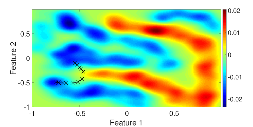
(a)

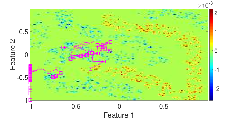
(b)

Figure 2. Heatmaps visualising decision boundaries of RBF SVM’s trained on a sample dataset. (a) $\gamma=10^{2}$ model: two black curves display attack paths under gradient descent, of two target points reaching the decision boundary; (b) $\gamma=10^{4}$ model: two magenta curves display attack paths under gradient descent, of the two target points now move away from the boundary or take significantly more steps.

where $\{(\boldsymbol{x}_{i},y_{i}),i=1,\ldots,n\}$ is the training data with $\boldsymbol{x}_{i}\in\mathbb{R}^{n}$ and $y_{i}\in\{-1,1\}^{n}$, $\boldsymbol{\alpha}$ are Lagrange multipliers, $\boldsymbol{0}$, $\boldsymbol{1}$ the all zeros, ones vectors, $C>0$ the regularisation penalty parameter on misclassified samples, and $\boldsymbol{\mathrm{G}}$ the $n\times n$ Gram matrix with entries $G_{ij}=y_{i}y_{j}k(\boldsymbol{x}_{i},\boldsymbol{x}_{j})$. The RBF kernel $k(\boldsymbol{x}_{i},\boldsymbol{x}_{j})=\exp(-\gamma\left\|\boldsymbol{x}_{i}-\boldsymbol{x}_{j}\right\|_{2}^{2})$ has precision parameter $\gamma>0$ that controls kernel width $\sqrt{2/\gamma}$. By the Representer Theorem, the learned classifier

(3) $$f(\boldsymbol{x}) = \sum_{i=1}^{n}\alpha_{i}y_{i}k(\boldsymbol{x}_{i},\boldsymbol{x})+b\enspace.$$

Adequacy and Improvements to Gradient-Descent Method. While the gradient-descent method has been effective against a number of machine learning models, e.g., DNNs, linear SVMs, logistic regression (Biggio et al., 2013; Goodfellow et al., 2014; Moosavi-Dezfooli et al., 2016a; Nguyen et al., 2015; Papernot et al., 2016b), there is no general guarantee that gradient descent converges to a global minimum of $f(\cdot)$ or even converges to local optima quickly—relevant to computational complexity (a measure of hardness) of evasion. Under linear models—a major focus of past work—gradient descent quickly finds global optima. While DNNs have been argued to exhibit local linearity, the existing body of evidence is insufficient to properly assess the effectiveness of the attack approach. As we argue in the next section, the approach is in fact unlikely to be successful against certain SVMs with RBF kernels, when kernel parameter $\gamma$ is chosen appropriately.

Problem 3.1.

What limitations of the gradient-descent method are to be expected when applied to evasion attacks?

Problem 3.2.

Are there simple defences to the gradient-descent method for popular learners?

Problem 3.3.

Are there more effective alternative approaches to generating adversarial samples?

We address each of these problems in this paper, with special focus on the RBF SVM as a case study and important example of where the most popular approach to evasion attack generation can predictably fail, and be improved upon.

4. Gradient-Descent Method Failure Modes

In this section, we explore how the gradient-descent method can fail against RBF SVMs with small kernel widths.

Illustrative Example. To demonstrate our key observation, we trained two RBF SVMs on a toy two-class dataset comprising two features (Chang and Lin, 2011, 2016), using two distinct values for $\gamma$: $10^{2}$ and $10^{4}$. Figure 2 displays the heatmaps of the two models’ decision functions. As can be seen, for the larger $\gamma$ case, additional regions result with flat, approximately-zero, decision values. Since the gradients in these regions are vanishingly small, it is significantly more likely that an iterate in the gradient-descent method’s attack trajectory will become trapped, or even move towards a direction away from the decision boundary altogether. Notably, both models achieve test accuracies of 100%.

In Figure 2(a), the two black curves marked with crosses demonstrate how two initial target points $(-0.55,-0.1)$ and $(-0.75,-0.5)$, move towards the decision boundary following the gradient-descent method. However, the two magenta curves marked with squares in Figure 2(b) demonstrate how the same two points either move away from the boundary or take significantly more steps to reach it, following the same algorithm but under a different model with a much larger $\gamma$.

This example illustrates that although the gradient-descent method makes the test sample less similar to the original class, it does not necessarily become similar to the other class.

Discussion. We employ Figure 3 to further explain possible failure modes of the gradient-descent method: points may get stuck or even move in the wrong direction. In this given 2D case, $\boldsymbol{x}_{1}$ belongs to Class 1, and $\boldsymbol{x}_{2}$ to Class 2. At instance $\boldsymbol{x}$, the $k^{th}$ component of the gradient is $\nabla^{k}f(\boldsymbol{x})=\sum_{i=1}^{2}2\gamma\alpha_{i}y_{i}(x_{i}^{k}-x^{k})\cdot\exp(-\gamma\left\|\boldsymbol{x}-\boldsymbol{x}_{i}\right\|_{2}^{2})$. Clearly, the sign of $\nabla^{k}$ can be flipped by various choices of $\gamma$. Suppose $x_{1}^{1},\,x_{2}^{1}>x^{1}$, then solving for $\nabla^{1}=0$, we obtain the point at which this phase transition occurs as:

$$\gamma = \frac{\log\alpha_{1}(x_{1}^{1}-x^{1})-\log\alpha_{2}(x_{2}^{1}-x^{1})}{\left\|\boldsymbol{x}-\boldsymbol{x}_{1}\right\|_{2}^{2}-\left\|\boldsymbol{x}-\boldsymbol{x}_{2}\right\|_{2}^{2}}\enspace.$$

Figure 3. Gradient-descent method failure modes.

The failure modes hold true in multiclass scenarios. For test sample $\boldsymbol{x}$ the classifier evaluates an $f_{i}(\boldsymbol{x})$ per class $i$ and selects the maximiser (a one-vs-all reduction). Suppose that $f_{1}(\boldsymbol{x})$ and $f_{2}(\boldsymbol{x})$ are the highest class scores. If $\gamma$ is chosen appropriately as above, then gradient descent reduces both $f_{1}(\boldsymbol{x})$ and $f_{2}(\boldsymbol{x})$ without ever reranking the two classes.

Figure 3 presents a geometric explanation, where distance between support vectors of opposite classes exceeding kernel width results in gradient-descent method iterates becoming trapped in the “gap” between. This section partially addresses Problem 3.1 through the discussed limitations, while setting $\gamma$ can provide a level of defence per Problem 3.2.

5. The Gradient-Quotient Method

The previous section motivates Problem 3.3’s search for effective alternatives to decreasing current class $i$ $f_{i}(\boldsymbol{x})$ while increasing desired class $j$ $f_{j}(\boldsymbol{x})$. Rather than moving in the direction $-\nabla f_{i}(\boldsymbol{x})$ as the gradient-descent method does (noting this is in the subgradient for the one-vs-all reduction), we propose following the gradient of the quotient $-f_{i}(\boldsymbol{x})/f_{j}(\boldsymbol{x})$:

$$\boldsymbol{x}_{t+1} = \boldsymbol{x}_{t}-\varepsilon_{t}\cdot\nabla(f_{i}(\boldsymbol{x})/f_{j}(\boldsymbol{x}))\enspace.$$

Remark 1.

Employing $f_{i}(\boldsymbol{x})-f_{j}(\boldsymbol{x})$ in place of $f_{i}(\boldsymbol{x})/f_{j}(\boldsymbol{x})$ does not achieve the desired result by the same flaws suffered by the gradient-descent method: $f_{i}(\boldsymbol{x}),f_{j}(\boldsymbol{x})$ and $f_{i}(\boldsymbol{x})-f_{j}(\boldsymbol{x})$ are decreased simultaneously, while $f_{i}(\boldsymbol{x})$ can remain larger than $f_{j}(\boldsymbol{x})$, with no misclassification occurring.

Note that while in the above, $i$ is taken as the current (maximising) class index, taking $j$ as the next highest-scoring class corresponds to evasion attacks while taking $j$ as any fixed target class corresponds to a mimicry attack. The results of Section 7 establish that this method can be more effective for manipulating test data in multiclass settings. However, it is not appropriate to binary-class cases as $-f_{1}(\boldsymbol{x})/f_{2}(\boldsymbol{x})=1$.

Step Size. The step size $\varepsilon_{t}$ is important to select carefully: too small and convergence slows; too large and the attack incurs excessive $L_{1}$ change, potentially exposing the attack.

Input : Iterate $\boldsymbol{x}_{t}$; Current quotient gradient $\nabla\in\mathbb{R}^{d}$; Parameter $\eta>0$

Output : Step size $\varepsilon_{t}$

1 Select $i\in\arg\max_{j\in[d]}|\nabla^{j}|$.

2Select $\varepsilon_{t}>0$ such that $\varepsilon_{t}\cdot|\nabla^{i}|\in\sqrt{t}[5\eta,10\eta]$.

Algorithm 1 Gradient-quotient step size.

In our experiments, we limit the largest change made to a single feature per iteration, and determine the step size accordingly as described in Algorithm 1. Here $\eta$ is a domain-specific value corresponding to a unit change in a feature, e.g., for a grayscale image $\eta=1$ corresponds to a unit change intensity level. The select rule’s $[5\eta,10\eta]$ is motivated by round-off practicalities in steps: if the largest gradient component were smaller than $5\eta$, it is likely that most other components would be 0, making convergence extremely slow. Since $[5\eta,10\eta]$ is a relatively conservative start, we increase it gradually; as explained next, the maximum step number in our experiments is 30. This increasing step size corresponds to a variant of guess-then-double. In addition, another advantage of Algorithm 1 is that it produces a similar amount of $L_{1}$ changes to the test samples, despite different values of $\gamma$.

6. Experiments: Gradient-Descent Method

Section 4 demonstrates that RBF SVM is less vulnerable to evasion attacks when $\gamma$ is set appropriately. In this section, we present a more detailed analysis of the impact of $\gamma$ on the attack’s success rate, further addressing Problems 3.1 and 3.2.

6.1. Datasets

Three datasets are selected to facilitate the analysis on $\gamma$: (1) MNIST (LeCun et al., 1998a, b) is a dataset of handwritten digits that has been widely studied. It contains a training set of $6\times 10^{4}$ samples (only the first $5\times 10^{4}$ are used in our experiments), and a test set of $10^{4}$ samples. Following the approach of (Papernot et al., 2016a), we divide the training set into 5 subsets of $10^{4}$ samples, $D_{1}\sim D_{5}$. Each subset is used to train models separately. Specifically, in the experiments that study binary-class settings, only the data in $D_{1}$ (or the test dataset) that belong to the two classes are used for training (or testing respectively). (2) USPS (Tibshirani, 2009) is another dataset of (normalised) handwritten digits scanned from envelopes by the U.S. Postal Service. There are 7291 training observations and 2007 test observations, each of which is a 16 $\times$ 16 grayscale image. (3) Spambase (Lichman, 2013) contains a total number of 4601 emails, with 1813 (2788) being spam (non-spam). In our experiments, we randomly select 3000 emails as the training set, and the remainder as the test set. Table 1 summarises the key information of these three datasets. Note that MNIST and Spambase are scaled to [0,1], while USPS is scaled to [-1, 1].

Table 1. Summary of the datasets used in this paper

Name	Size		Features	Domain	Range
	Training set	Test set
MNIST	$5\times 10^{4}$	$10^{4}$	$28\times 28$	Vision	[0, 1]
USPS	7291	2007	$16\times 16$	Vision	[-1, 1]
Spambase	3000	1601	57	Spam	[0, 1]

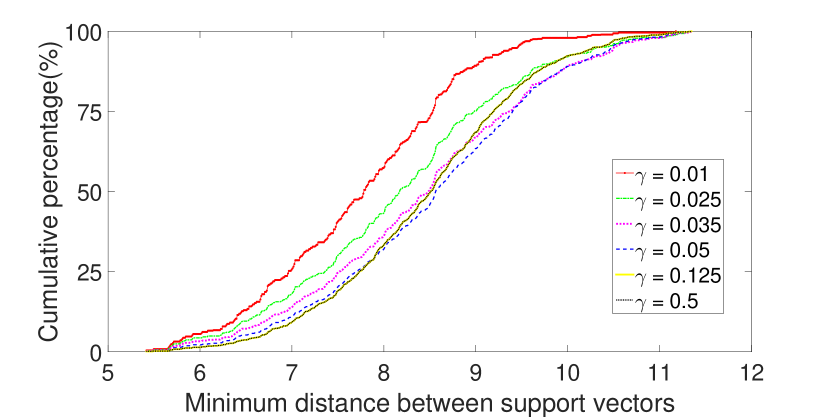
Figure 4. Minimum distance between each support vector of class “3” and all support vectors of class “4” in the MNIST dataset.

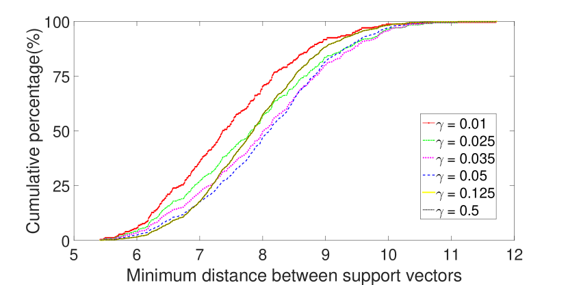
Figure 5. Minimum distance between each support vector of class “4” and all support vectors of class “3” in the MNIST dataset.

6.2. Impact of $\gamma$ on Vulnerability (Binary Class)

We begin with the binary scenario and investigate how $\gamma$ impacts the success rate of causing SVMs to misclassify (1) three pairs of digits—1 & 2, 3 & 4, 5 & 7 for the MNIST dataset, (2) three pairs of digits—0 & 1, 2 & 3, 6 & 7 for the USPS dataset, and (3) spam and non-spam emails for the Spambase dataset. Note that in this subsection, all models regarding the MNIST dataset are trained on $D_{1}$. An attack is considered successful if the perturbed test sample is misclassified within 30 steps. The reason why we choose 30 is that although larger values will increase the attack’s success rate, the changes made to the original samples are so obvious they would be easily detected by manual audit.

Tables 2(a)–2(c), 3(a)–3(c) and 4 illustrate a phase transition in all cases: a small decrease of $\gamma$ causes a significant jump in success rate. Figure 6 visualises the phase transition.

From the attacker’s point of view, in addition to minimising the overall changes, it is also desirable that no single pixel is modified by a large amount when perturbing an image, i.e., $\left\|\boldsymbol{\delta}\right\|_{\infty}<B_{\infty}\in R^{+}$ ($B_{\infty}$ can be considered as the attacker’s budget). Therefore, we modify the original optimisation problem 1 as follows:

(4) $$\arg\min_{\boldsymbol{\delta}\in\mathbb{R}^{d}} \left\|\boldsymbol{\delta}\right\|_{1}$$

s.t. $$\mathrm{sgn}(f(\boldsymbol{x}))\neq\mathrm{sgn}(f(\boldsymbol{x}+\boldsymbol{\delta}))$$

$$\left\|\boldsymbol{\delta}\right\|_{1}<B_{1}\in R^{+},$$

$$\left\|\boldsymbol{\delta}\right\|_{\infty}<B_{\infty}\in R^{+}$$

We apply much stricter stopping criteria, and re-run the experiments on MNIST and USPS. As can be seen from Tables 5 & 6, a phase transition still exists in each case.

Table 2. Success rate and average $L_{1}$ change for gradient-descent method evasion attacks (binary class, MNIST).

(a) RBF SVM: MNIST, digits 1 and 2.

$\gamma$		0.01	0.02	0.025	0.05	0.1	0.11	0.125	0.5
$C$		$5\times 10^{4}$	$5\times 10^{4}$	$5\times 10^{4}$	$5\times 10^{4}$	$5\times 10^{4}$	$5\times 10^{4}$	$5\times 10^{4}$	10
Accuracy(%)		99.4	99.5	99.6	99.5	99.8	99.7	99.5	98.6
$1\to 2$	Succ rate (%)	100	100	100	100	90.1	68.9	36.3	1.5
	$P(2/\sqrt{\gamma}\geq MinDist)$ (%)	100	100	100	100	68.4	55.0	35.0	0.1
$2\to 1$	Succ rate (%)	94.1	68.9	54.8	17.0	11.3	13.3	15.2	12.9
	$P(2/\sqrt{\gamma}\geq MinDist)$ (%)	100	100	100	59.3	7.5	4.8	2.8	0.1

(b) RBF SVM: MNIST, digits 3 and 4.

$\gamma$		0.01	0.025	0.035	0.05	0.125	0.5
$C$		$10^{4}$	$10^{4}$	$10^{4}$	$10^{4}$	$10^{4}$	10
Accuracy(%)		99.5	99.7	99.6	99.5	99.5	99.8
$3\to 4$	Succ rate (%)	100	94.5	76.0	53.4	14.8	5.3
	$P(2/\sqrt{\gamma}\geq MinDist)$ (%)	100	100	96.7	61.7	0.29	0.1
$4\to 3$	Succ rate (%)	100	100	98.1	82.5	11.8	1.6
	$P(2/\sqrt{\gamma}\geq MinDist)$ (%)	100	100	99.2	79.7	0.4	0.1

(c) RBF SVM: MNIST, digits 5 and 7.

$\gamma$		0.01	0.025	0.035	0.05	0.1	0.5
$C$		$10^{4}$	$10^{4}$	$10^{4}$	$10^{4}$	$10^{4}$	10
Accuracy(%)		99.3	99.5	99.6	99.6	99.1	99.7
$5\to 7$	Succ rate (%)	100	97.0	87.4	71.1	41.8	6.2
	$P(2/\sqrt{\gamma}\geq MinDist)$ (%)	100	100	98.7	75.6	0.2	0.1
$7\to 5$	Succ rate (%)	100	100	99.8	91.1	15.5	2.3
	$P(2/\sqrt{\gamma}\geq MinDist)$ (%)	100	100	100	87.2	0.2	0.1

(d) Linear SVM.

	$C=1000$			$C=5000$
	Succ rate (%)	Ave $L_{1}$ change	Accuracy (%)	Succ rate (%)	Ave $L_{1}$ change	Accuracy (%)
$1\to 2$	100	22.8	99.3	100	18.4	99.2
$2\to 1$	100	37.5		100	34.8
$3\to 4$	100	39.5	99.7	100	37.3	99.6
$4\to 3$	100	32.8		100	25.9
$5\to 7$	100	30.4	99.0	100	28.1	99.0
$7\to 5$	100	29.1		100	23.6

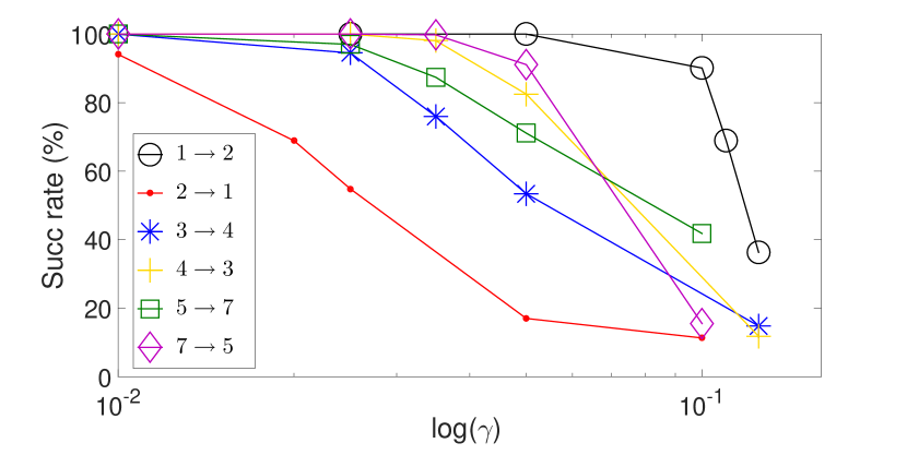
(a) MNIST

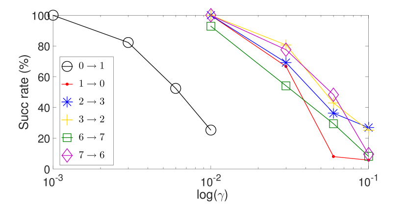
(b) USPS

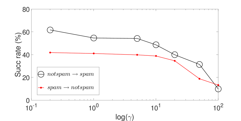
(c) Spambase

Figure 6. Phase transition of the success rate for gradient-descent method evasion attacks.

Table 3. Success rate for gradient-descent method evasion attacks (binary class, USPS).

(a) RBF SVM: USPS, digits 0 and 1.

$\gamma$		0.001	0.003	0.006	0.01	0.03	0.06	0.1
$C$		$10^{4}$	$10^{4}$	$10^{4}$	$5\times 10^{3}$	$5\times 10^{3}$	$5\times 10^{3}$	$10^{3}$
Accuracy(%)		99.2	99.5	99.4	99.5	99.5	99.4	99.4
$0\to 1$	Succ rate (%)	100	82.3	52.4	25.3	4.7	3.4	3.6
	$P(2/\sqrt{\gamma}\geq MinDist)$ (%)	100	100	100	100	35.7	6.0	0.6
$1\to 0$	Succ rate (%)	100	100	100	100	66.7	8.0	5.7
	$P(2/\sqrt{\gamma}\geq MinDist)$ (%)	100	100	100	100	100	98.3	22.0

(b) RBF SVM: USPS, digits 2 and 3.

$\gamma$		0.01	0.03	0.06	0.1
$C$		$10^{5}$	$10^{5}$	$10^{5}$	$10^{5}$
Accuracy(%)		97.5	97.8	97.8	97.8
$2\to 3$	Succ rate (%)	100	69.2	36.3	26.9
	$P(2/\sqrt{\gamma}\geq MinDist)$ (%)	100	97.9	45.4	4.6
$3\to 2$	Succ rate (%)	100	80.7	42.9	25.2
	$P(2/\sqrt{\gamma}\geq MinDist)$ (%)	100	100	52.1	11.1

(c) RBF SVM: USPS, digits 6 and 7.

$\gamma$		0.01	0.02	0.03	0.06
$C$		$10^{4}$	$10^{4}$	$10^{4}$	$10^{4}$
Accuracy(%)		99.7	99.7	99.7	99.7
$6\to 7$	Succ rate (%)	92.9	54.1	29.4	8.2
	$P(2/\sqrt{\gamma}\geq MinDist)$ (%)	100	99.2	65.9	19.4
$7\to 6$	Succ rate (%)	100	77.6	48.3	9.6
	$P(2/\sqrt{\gamma}\geq MinDist)$ (%)	100	100	86.5	24.3

Table 4. Success rate for gradient-descent method evasion attacks (binary class, Spambase).

$\gamma$		0.2	1	5	10	20	50	100
$C$		$5\times 10^{5}$	$5\times 10^{5}$	$10^{5}$	$10^{5}$	$10^{5}$	$10^{5}$	$5\times 10^{4}$
Accuracy(%)		91.3	92.9	92.9	92.9	92.6	92.1	91.4
$0\to 1$a	Succ rate (%)	61.7	54.6	54.2	48.6	39.9	31.4	9.9
	$P(2/\sqrt{\gamma}\geq MinDist)$ (%)	100	99.9	94.5	86.8	73.3	53.6	41.8
$1\to 0$	Succ rate (%)	41.8	41.0	39.8	38.8	34.6	18.8	13.3
	$P(2/\sqrt{\gamma}\geq MinDist)$ (%)	100	100	97.7	94.6	89.4	64.6	41.7

• 0: not spam, 1: spam

Table 5. Success rate of gradient-descent method evasion attacks (binary class, MNIST, with $L_{1}$ and $L_{\infty}$ limit)

(a) digits 1 and 2, $B_{1}$=39.2, $B_{\infty}$=0.3

$\gamma$		0.01	0.05	0.1
$C$		$5\times 10^{4}$	$5\times 10^{4}$	$5\times 10^{4}$
Accuracy (%)		99.4	99.5	99.8
Succ rate (%)	$1\to 2$	99.5	92.7	30.4
	$2\to 1$	27.2	8.4	9.8

(b) digits 3 and 4, $B_{1}$=39.2, $B_{\infty}$=0.3

$\gamma$		0.01	0.05	0.125
$C$		$10^{4}$	$10^{4}$	$10^{4}$
Accuracy (%)		99.5	99.5	99.5
Succ rate (%)	$3\to 4$	34.5	18.8	12.5
	$4\to 3$	44.4	24.3	6.1

(c) digits 5 and 7, $B_{1}$=39.2, $B_{\infty}$=0.3

$\gamma$		0.01	0.05	0.1
$C$		$10^{4}$	$10^{4}$	$10^{4}$
Accuracy (%)		99.3	99.6	99.1
Succ rate (%)	$5\to 7$	48.8	24.2	25.7
	$7\to 5$	51.6	22.8	7.1

Table 6. Success rate of gradient-descent method evasion attacks (binary class, USPS, with $L_{1}$ and $L_{\infty}$ limit)

(a) digits 0 and 1, $B_{1}$=76.8, $B_{\infty}$=0.6

$\gamma$		0.001	0.01	0.03	0.06
$C$		$10^{4}$	$5\times 10^{3}$	$5\times 10^{3}$	$5\times 10^{3}$
Accuracy (%)		99.2	99.5	99.5	99.4
Succ rate (%)	$0\to 1$	22.2	10.9	4.7	3.1
	$1\to 0$	100	100	29.5	8.8

(b) digits 2 and 3, $B_{1}$=51.2, $B_{\infty}$=0.3

$\gamma$		0.01	0.03	0.06	0.1
$C$		$10^{5}$	$10^{5}$	$10^{5}$	$10^{5}$
Accuracy (%)		97.8	97.8	97.8	97.8
Succ rate (%)	$2\to 3$	50.3	34.2	25.4	20.2
	$3\to 2$	52.5	38.7	25.2	12.9

(c) digits 6 and 7, $B_{1}$=76.8, $B_{\infty}$=0.6

$\gamma$		0.01	0.02	0.03	0.06
$C$		$10^{4}$	$10^{4}$	$10^{4}$	$10^{4}$
Accuracy (%)		99.7	99.7	99.7	99.7
Succ rate (%)	$6\to 7$	58.9	38.2	19.4	7.6
	$7\to 6$	80.8	52.1	26.0	8.2

Inter-Class-SV Distance. Since $\gamma$ controls how quickly the RBF kernel vanishes, we are motivated to compare minimum (Euclidean) distance between each support vector of one class $(sv_{1i})$ and all support vectors of the opposite class $(sv_{2j})$, i.e., $MinDist(sv_{1i})=\arg\min_{j}\,Distance(sv_{1i},sv_{2j})$. Our intuition is that a larger $\gamma$ suggests (1) a quicker drop of values for both the kernel function and the gradient; (2) a wider gap between the two classes. Both observations contribute to the lower success rate of the evasion attack.

Figures 5 and 5 present the minimum distance between support vectors of classes “3” and “4” in the MNIST dataset (due to similarities, we omit the other results). Observe that when $\gamma$ first decreases from 0.5, the support vectors of the opposite class move further away—here the corresponding model is still less vulnerable to evasion attack. As $\gamma$ continues to decrease the trend reverses, i.e., the support vectors of opposite class move closer to each other. A smaller $\gamma$ already means the RBF kernel vanishes more slowly, and the closer distance between the two classes makes it even easier for a test sample to cross the decision boundary. Consequently, the corresponding model becomes much more vulnerable.

This prompts the question: Given a model with a $\gamma$, is there a way to determine whether the model is robust? The results in Tables 2(a)–2(c), 3(a)–3(c) and 4 witness a strong correlation between success rate and the percentage of “$2/\sqrt{\gamma}\geq$ minimum distance”—the lower the percentage the less vulnerable the model.

Margin Explanation. We have also observed a positive correlation between margin per support vector and the minimum distance calculated above. These findings suggest that separated inter-class support vectors lead to more secure models, lending experimental support to the geometric argument (Section 4).

Linear SVM. The experiments are performed for linear SVMs on MNIST, with results serving as baseline. Table 2(d) demonstrates that success rates under linear models are 100%, as expected. However, a larger $C$ requires smaller changes to the target sample, as larger $C$ leads to smaller margin.

Discussion on model robustness vs. overfitting. It should be noted that we are not suggesting larger $\gamma$ induces robustness. Instead, we demonstrate a phrase transition with small increase to $\gamma$ causes significant success rate drop for evasion attacks. Further increase to $\gamma$ over the threshold value offers little benefit. Our current results suggest that the model may (Table 4) or may not (Tables 2,  3) overfit when $\gamma$ reaches the threshold value.

6.3. Impact of $\gamma$ on Vulnerability (Multiclass)

This section further investigates the impact of $\gamma$ on success rate of evasion attacks, in multiclass scenarios. For the MNIST dataset, two RBF SVMs with $\gamma$ as 0.05 and 0.5, are trained on both $D_{1}$ and $D_{2}$, respectively. For comparison, four linear SVMs are also trained on $D_{1}$ and $D_{2}$ with different values of $C$. For the USPS dataset, three RBF SVMs are trained, where $\gamma$ = 0.02, 0.1 and 0.5. An attack is still considered successful if the perturbed test sample is misclassified within 30 steps.

As can be seen from Tables 6.3 and 8: (1) for RBF SVMs, the success rates under the models with larger $\gamma$ are much lower; (2) for linear SVMs the success rates are always 100%, but the average $L_{1}$ change is smaller as $C$ increases—observations consistent with previous results.

Table 7. Success rate and average $L_{1}$ change of gradient-descent method evasion attack, in multiclass scenarios, MNIST^a

		Accuracy (%)	Succ rate (%)	1.6cmAve $L_{1}$
change
RBF  $(\gamma=0.05,\,C=10^{3})$	Model 1	87.2	91.8	$39.4^{b}$
	Model 2	87.7	92.8	$40.5^{b}$
RBF  $(\gamma=0.5,\,C=10)$	Model 1	94.8	24.4	$17.7^{b}$
	Model 2	94.8	23.7	$18.2^{b}$
Linear $(C=10^{3})$	Model 1	89.0	100	28.5
	Model 2	89.2	100	26.8
Linear $(C=2\times 10^{4})$	Model 1	91.4	100	18.7
	Model 2	91.7	100	18.1

• Since it takes more than an order of magnitude longer to run experiments using RBF SVM than linear kernel, each result regarding RBF SVM is based on 1000 test samples, while each linear SVM result is based on 5000 test samples.

• Only the successful cases are counted.

Table 8. Success rate and average $L_{1}$ change of gradient-descent method evasion attack, in multiclass scenarios, USPS^a

$\gamma$	$C$	Accuracy (%)	Succ rate (%)	Ave $L_{1}$ change
0.02	$10^{4}$	89.9	89.6	$42.5^{b}$
0.1	$2\times 10^{3}$	92.1	38.7	$40.7^{b}$
0.5	$10^{2}$	95.0	38.2	$40.9^{b}$

• Each result is based on 1500 test samples.

• Only the successful cases are counted.

7. Experiments: Gradient-Quotient Method

In this section we present experimental results establishing the effectiveness of our proposed method for generating adversarial samples.

7.1. Attacking SVMs & RBF Networks Directly

Recall that based on our new approach, a test sample $\boldsymbol{x}$ is updated as $\boldsymbol{x}_{t+1}=\boldsymbol{x}_{t}-\varepsilon_{t}\cdot\nabla(f_{1}(\boldsymbol{x})/f_{2}(\boldsymbol{x}))$, where $f_{1}(\boldsymbol{x})$ and $f_{2}(\boldsymbol{x})$ are the scores for the top two scoring classes for $\boldsymbol{x}$. In order to test whether this method is more effective than the popular gradient-descent method, we run similar experiments to Section 6.3, (1) for the MNIST dataset, one RBF SVM $(\gamma=0.5,C=10)$ and one linear SVM $(C=1000)$ are trained on $D_{1},D_{2},\ldots,D_{5}$, respectively; (2) for the USPS dataset, the RBF SVM with $\gamma=0.5,C=10^{2}$ is reused.

Comparing the results in Table 6.3 and Table 7.1, we observe that the gradient quotient method is very effective against SVMs trained on the MNIST dataset: (1) for the RBF SVMs with $\gamma=0.5$, the success rates increase from around 24% to a resounding 100%. Moreover we have tested a wide range of values for $\gamma$ from 0.01 through 10, with resulting success rates always 100% under our new approach; (2) the required $L_{1}$ perturbation also decreases.

However, the new method achieves a success rate of only 71.2% (still higher than the gradient descent method’s 38.2%) against the RBF SVM trained on the USPS dataset. An examination of the log files reveals that in this case, the second highest score $f_{2}$ is always negative, and hence decreasing the quotient of $f_{1}/f_{2}$ may not work. Interestingly, such finding coincides with our previous conclusion that models with wider inter-class gap are more robust.

Attacking RBF networks. Does the gradient quotient method work with other types of model? We further test it against a RBF network trained on $D_{1}$, with 600 RBF neurons and a learning rate of 0.05. The results show that the success rate is 74.1% ($f_{2}$ is also negative in this case), which is slightly lower than the gradient descent method’s 79.9%.

In summary, the proposed gradient quotient method works most effectively when the scores for both the original and target classes are positive. In other situations, it performs at least similarly to the gradient descent method—none of our experimental results on all datasets and two types of models has shown any obvious inferiority.

Table 9. Success rate and average $L_{1}$ change of the evasion attack (the gradient quotient method, multiclass scenarios, MNIST).^a

		Accuracy (%)	Succ rate (%)	1.6cmAve$L_{1}$
change
RBF $(\gamma=0.5,$ $C=10)$	Model 1	94.8	100	17.8
	Model 2	94.8	100	17.9
	Model 3	95.0	100	17.4
	Model 4	95.2	100	17.5
	Model 5	95.0	100	18.1
Linear $(C=10^{3})$	Model 1	89.0	100	19.3
	Model 2	89.2	100	20.6
	Model 3	89.1	100	20.9
	Model 4	89.2	100	20.8
	Model 5	88.9	100	19.9

• Each result regarding RBF SVM is based on 800 test samples, while each result on linear SVM is based on 5000 test samples.

7.2. Attacking via Surrogate

Up until now, we have implicitly assumed that the attacker possesses complete knowledge of the target classifier, which may be unrealistic in practice. Hence, we next examine attacks carried out via a surrogate. For example, in order to mislead a RBF SVM, the attacker first trains their own RBF SVM on a similar dataset, builds the attack path of how a test sample should be modified, then applies it to the target SVM.

Since there is no guarantee that the surrogate and target classifiers misclassify the test sample simultaneously, all test samples are modified 15 times by the surrogate in this experiment; an attack is considered to be successful if the target classifier misclassifies the adversarial sample within 15 steps too. In addition, we modify the method as:

$$\boldsymbol{x}_{t+1}=\begin{cases}\boldsymbol{x}_{t}-\varepsilon_{t}\cdot\nabla(f_{1}(\boldsymbol{x}_{t})/f_{2}(\boldsymbol{x}_{t}))&\text{ prior to surrogate}\\ &\text{ misclassification}\\ \boldsymbol{x}_{t}+\varepsilon_{t}\cdot\nabla(f_{1}(\boldsymbol{x}_{t})/f_{2}(\boldsymbol{x}_{t}))&\text{ otherwise}\end{cases}$$

In other words, before the test sample is misclassified by the surrogate, it travels “downhill”, but after crossing the decision boundary it travels “uphill”. Otherwise the test case continues oscillating back and forth around the boundary.

Intra-model transferability. We reuse the RBF SVMs trained on $D_{1},D_{2},\ldots,D_{5}$, each of which serving as both surrogate $(S_{i})$ and target $(T_{i})$ classifiers. As can be seen from Table 10, the success rates are all over 65%. Specifically, those values inside the bracket are the success rates when the target classifier misclassifies before the surrogate, while the values outside are the overall success rates. For comparison, the same experiments have been performed for linear SVMs, producing similar success rates (54%—71%), notably higher than previous findings (around 40%) reported by Papernot et al. (2016a).

Table 10. Success rate of evasion attacks via surrogate (RBF SVM, MNIST).^a

	$T_{1}$	$T_{2}$	$T_{3}$	$T_{4}$	$T_{5}$
$S_{1}$	100	66.1 (9.2)	69.8 (9.5)	68.3 (9.8)	66.4 (7.1)
$S_{2}$	68.0 (8.2)	100	67.2 (8.4)	72.4 (10.4)	67.9 (7.4)
$S_{3}$	65.0 (8.4)	66.1 (9.4)	100	67.3 (11.1)	65.9 (8.5)
$S_{4}$	65.3 (10.0)	67.2 (10.8)	67.0 (10.6)	100	65.3 (8.8)
$S_{5}$	67.0 (9.2)	67.8 (8.9)	69.4 (9.0)	69.4 (9.1)	100

• Each result is based on 800 test samples.

Inter-model transferability. Is gradient quotient based evasion attack still effective if the surrogate and target models are of different types? We keep the above five RBF SVMs as surrogate, but change the target classifier to the RBF network (trained on $D_{1}$) from the last subsection. The results show that the success rates range from 61.3% to 69.1%, which are very close to the values in Table 10.

7.3. Mimicry Attacks

The previous two subsections have demonstrated that our new approach is effective in manipulating test samples. But what if the attacker intends to make the test sample misclassified as a specific class?

In order to test the gradient quotient method for mimicry attacks, we make the following change: $\boldsymbol{x}_{t+1}=\boldsymbol{x}_{t}-\varepsilon_{t}\cdot\nabla(f_{1}(\boldsymbol{x})/f_{T}(\boldsymbol{x}))$, where $f_{T}(\boldsymbol{x})$ corresponds to the score of the target class, while $f_{1}(\boldsymbol{x})$ is still the score for the top scoring class.

For each test sample in the MNIST dataset, we apply the gradient quotient algorithm to check whether it can be misclassified as each of the other nine digits. The RBF SVM $(\gamma=0.5,C=10)$ and the linear SVM ($C$ = 1000) trained on $D_{1}$ are reused here. The results in Figure 7 show that in most cases this approach can successfully make the original digit misclassified as the target. However, under the RBF SVM, the success rate is very low when the attack is to make other digits look like “0”. The reason is still that $f_{0}(\boldsymbol{x})$, i.e., the score for digit “0”, is always negative.

Another interesting point is that among the successful cases where other digits are misclassified as “0”, over half of them are digit “6”. Therefore, we tried an indirect method—first modify the test sample so that it is considered as “6” (the success rate for this step is 100%), and then follow the original method, i.e., modify “6” until either it is classified as “0”, or the maximum step limit of 30 is reached. This indirect approach doubled the overall success rate.

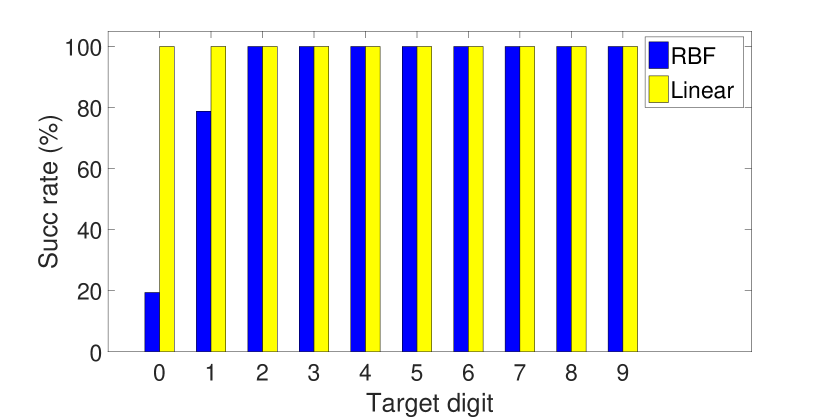
(a) Success rate

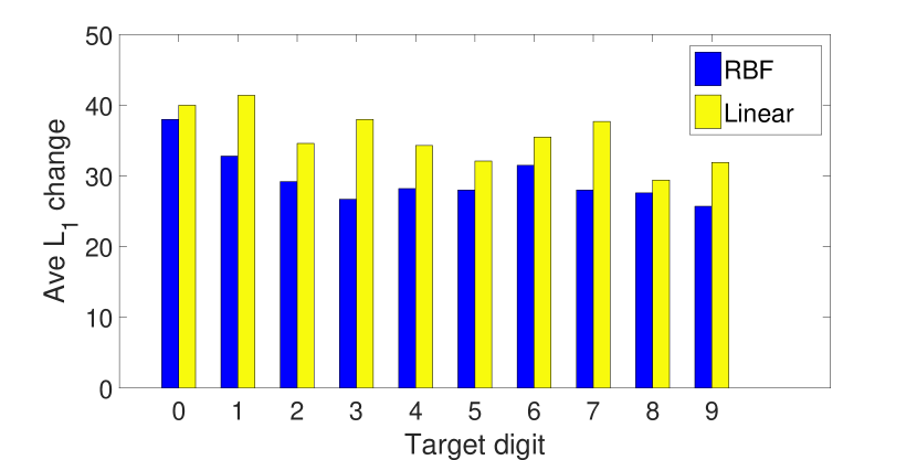
(b) $L_{1}$ change

Figure 7. Success rate and $L_{1}$ change of mislabelling other digits as the target digit.

8. Conclusions and Future Work

Recent studies have shown that it is relatively easy to fool machine learning models via adversarial samples. In this paper, we demonstrate that the gradient-descent method—the leading approach to generate adversarial samples—has limitations against RBF SVMs, when the precision parameter $\gamma$ controlling kernel smoothness is chosen properly. We find predictable phase transitions of attack success occur at thresholds that are functions of geometric margin-like quantities measuring inter-class support vector distances. Our characterisation can be used to make RBF SVM more robust against common evasion and mimicry attacks.

We propose a new method for manipulating target samples into adversarial instances, with experimental results showing that this new method not only increases attack success rate, but decreases the required changes made to input points.

For future work, (1) regarding the gradient-descent method, we intend to replicate and expand findings for $\gamma$ and smoothness in general, in other settings and for other classifiers. (2) We will continue exploring suitability of our new generation approach when the target is not an SVM, with direct attacks or SVM surrogates. (3) Further investigation into light-weight yet efficient countermeasures also serves as an important direction for future work.

References

- (1)
- Alfeld et al. (2016) Scott Alfeld, Xiaojin Zhu, and Paul Barford. 2016. Data Poisoning Attacks against Autoregressive Models.. In AAAI. 1452–1458.
- Barreno et al. (2010) Marco Barreno, Blaine Nelson, Anthony D. Joseph, and J. D. Tygar. 2010. The Security of Machine Learning. Machine Learning 81, 2 (2010), 121–148.
- Barreno et al. (2006) Marco Barreno, Blaine Nelson, Russell Sears, Anthony D. Joseph, and J. D. Tygar. 2006. Can Machine Learning Be Secure?. In AsiaCCS. 16–25.
- Bhagoji et al. (2017) Arjun Nitin Bhagoji, Daniel Cullina, and Prateek Mittal. 2017. Dimensionality Reduction as a Defense against Evasion Attacks on Machine Learning Classifiers. arXiv:1704.02654 (2017).
- Biggio et al. (2013) Battista Biggio, Igino Corona, Davide Maiorca, Blaine Nelson, Nedim rndić, Pavel Laskov, Giorgio Giacinto, and Fabio Roli. 2013. Evasion Attacks against Machine Learning at Test Time. In ECML PKDD. 387–402.
- Biggio et al. (2014) Battista Biggio, Igino Corona, Blaine Nelson, Benjamin I. P. Rubinstein, Davide Maiorca, Giorgio Fumera, Giorgio Giacinto, and Fabio Roli. 2014. Security Evaluation of Support Vector Machines in Adversarial Environments. In Support Vector Machine Applications, Y. Ma and G. Guo (Eds.). Springer, 105–153.
- Biggio et al. (2012) Battista Biggio, Blaine Nelson, and Pavel Laskov. 2012. Poisoning Attacks Against Support Vector Machines. In ICML. 1807–1814.
- Brückner and Scheffer (2011) Michael Brückner and Tobias Scheffer. 2011. Stackelberg games for adversarial prediction problems. In KDD. 547–555.
- Carlini and Wagner (2016) Nicholas Carlini and David Wagner. 2016. Defensive Distillation is Not Robust to Adversarial Examples. arXiv:1607.04311 (2016).
- Carlini and Wagner (2017) Nicholas Carlini and David Wagner. 2017. Towards Evaluating the Robustness of Neural Networks. arXiv:1608.04644 (2017).
- Chang and Lin (2011) Chih-Chung Chang and Chih-Jen Lin. 2011. LIBSVM: A Library for Support Vector Machines. ACM Transactions on Intelligent Systems and Technology 2, 3 (2011), 1–27.
- Chang and Lin (2016) Chih-Chung Chang and Chih-Jen Lin. 2016. LIBSVM Data: Classification (Binary Class). https://www.csie.ntu.edu.tw/~cjlin/libsvmtools/datasets/binary.html#fourclass. (2016).
- Dalvi et al. (2004) Nilesh Dalvi, Pedro Domingos, Mausam, Sumit Sanghai, and Deepak Verma. 2004. Adversarial classification. In KDD. 99–108.
- Goodfellow et al. (2014) Ian J. Goodfellow, Jonathon Shlens, and Christian Szegedy. 2014. Explaining and Harnessing Adversarial Examples. eprint arXiv:1412.6572 (2014). http://arxiv.org/abs/1412.6572
- Gu and Rigazio (2015) Shixiang Gu and Luca Rigazio. 2015. Towards Deep Neural Network Architectures Robust to Adversarial Examples. arXiv:1412.5068 (2015).
- Huang et al. (2011) Ling Huang, Anthony D. Joseph, Blaine Nelson, Benjamin I. P. Rubinstein, and J. D. Tygar. 2011. Adversarial Machine Learning. In ACM AISec Workshop. 43–57.
- Huang et al. (2016) Ruitong Huang, Bing Xu, Dale Schuurmans, and Csaba Szepesvari. 2016. Learning with a Strong Adversary. arXiv:1511.03034 (2016).
- LeCun et al. (1998a) Yann LeCun, Leon Bottou, Yoshua Bengio, and Patrick Haffner. 1998a. Gradient-based Learning Applied to Document Recognition. Proc. IEEE 86, 11 (1998), 2278–2324.
- LeCun et al. (1998b) Yann LeCun, Corinna Cortes, and Christopher J.C. Burges. 1998b. The MNIST Database of Handwritten Digits. http://yann.lecun.com/exdb/mnist/. (1998).
- Li and Vorobeychik (2014) Bo Li and Yevgeniy Vorobeychik. 2014. Feature Cross-substitution in Adversarial Classification. In NIPS (NIPS’14). MIT Press, Cambridge, MA, USA, 2087–2095. http://dl.acm.org/citation.cfm?id=2969033.2969060
- Li et al. (2016) Bo Li, Yining Wang, Aarti Singh, and Yevgeniy Vorobeychik. 2016. Data Poisoning Attacks on Factorization-Based Collaborative Filtering. In NIPS. 1885–1893.
- Lichman (2013) M. Lichman. 2013. UCI Machine Learning Repository. https://archive.ics.uci.edu/ml/datasets/spambase. (2013).
- Lowd and Meek (2005) Daniel Lowd and Christopher Meek. 2005. Adversarial Learning. In KDD. 641–647.
- Luo et al. (2016) Yan Luo, Xavier Boix, Gemma Roig, Tomaso Poggio, and Qi Zhao. 2016. Foveation-based Mechanisms Alleviate Adversarial Examples. arXiv:1511.06292 (2016).
- Miyato et al. (2016) Takeru Miyato, Shin-ichi Maeda, Masanori Koyama, Ken Nakae, and Shin Ishii. 2016. Distributional Smoothing with Virtual Adversarial Training. arXiv:1507.00677 (2016).