Parametric instability in periodically perturbed dynamos

Abstract

We examine kinematic dynamo action driven by an axisymmetric large-scale flow that is superimposed with an azimuthally propagating non-axisymmetric perturbation with a frequency $\omega$. Although we apply a rather simple large-scale velocity field, our simulations exhibit a complex behavior with oscillating and azimuthally drifting eigenmodes as well as stationary regimes. Within these non-oscillating regimes we find parametric resonances characterized by a considerable enhancement of dynamo action and by a locking of the phase of the magnetic field to the pattern of the perturbation. We find an approximate fulfillment of the relationship between the resonant frequency $\omega_{\rm{res}}$ of the excitation and the eigenfrequency $\omega_{0}$ of the undisturbed system given by $\omega_{\rm{res}}=2\omega_{0}$, which is known from paradigmatic rotating mechanical systems and our prior study [Giesecke et al., Phys. Rev. E, 86, 066303 (2012)]. We find further, broader, regimes with weaker enhancement of the growth rates but without phase locking. However, this amplification regime arises only in case of a basic (i.e., unperturbed) state consisting of several different eigenmodes with rather close growth rates. Qualitatively, these observations can be explained in terms of a simple low-dimensional model for the magnetic field amplitude that is derived using Floquet theory.

The observed phenomena may be of fundamental importance in planetary dynamo models with the base flow being disturbed by periodic external forces like precession or tides and for the realization of dynamo action under laboratory conditions where imposed perturbations with the appropriate frequency might facilitate the occurrence of dynamo action.

I Introduction

Usually it is assumed that magnetic fields of galaxies, stars, and planets are generated by the magnetohydrodynamic dynamo effect, which describes the transfer of kinetic energy from a flow of an electrically conducting fluid into magnetic energy. Regarding stellar or planetary bodies, magnetic fields are supposed to be powered by convection-driven flows King et al. (2010). However, there are also alternative concepts for planetary dynamos with a flow driven by mechanical stirring, like precession (which has been considered as an alternative forcing for the geodynamo Malkus (1968) and the ancient lunar dynamo Dwyer et al. (2011); Noir and Cébron (2013)), or tidal forcing (which has been proposed to be responsible for the ancient Martian dynamo Arkani-Hamed et al. (2008) and, as well, for the early lunar dynamo Le Bars et al. (2011)).

Although mechanical stirring, whether by precession or by tides, is capable to drive a dynamo by its own Tilgner (2005); Cébron and Hollerbach (2014), it is more likely that in the case of realistic planetary models a combination of different types of forcing is responsible for the total flow, with tides and/or precession acting as a periodic perturbation to a base flow (e.g., convectively driven motions Ogilvie and Lesur (2012)). Despite the small amount of energy provided instantaneously by the perturbation flow, its impact can be large since the perturbation may act as a kind of catalyst that allows a transfer of energy from the available rotational energy, which is huge but does not contribute to magnetic induction, into a more usable form of flow Le Bars et al. (2015). In particular, a periodic perturbation of some base flow may cause a parametric resonance resulting, e.g., in the excitation of free nonaxisymmetric inertial waves like have been found in simulations and experiments of precession driven flows Kerswell (1999); Lorenzani and Tilgner (2003); Lagrange et al. (2011); Giesecke et al. (2015); Herault et al. (2017). Such time-dependent nonaxisymmetric flow perturbations in turn may significantly enhance the ability of the system to drive a dynamo via yet another resonance attributed to the magnetic field generation process by coupling low-order rotational modes of the fluid flow Aldridge et al. (2007).

A paradigmatic system related to the dynamo effect is the disk dynamo, in which a current is guided from the edge of a rotating conductive disk to the disk axis in such a way that the induced magnetic field amplifies the original (seed) field. A positive effect on magnetic self-excitation arises when periodically varying the rotation rate of the disk with an appropriate frequency Priede et al. (2010). Similar to periodically perturbed mechanical problems, this system can be described by a Mathieu equation, which represents a special case of the Hill equation

$$\frac{d^{2}y}{dt^{2}}=a(t)y$$ (1)

with $a(t+T)=a(t)$ being a $T-$periodic function. A parametric resonance occurs if the excitation frequency $\omega$ is twice the eigenfrequency $\omega_{0}$ of the unperturbed system, i.e., $\omega_{\rm{res}}=2\omega_{0}$. In this case the field generation of the disk dynamo is based on a simple axially symmetric variation of the velocity of a solid body. More relevant for astrophysical objects are fluid flow driven dynamos where the induced electrical currents have more degrees of freedom. In that case a perturbation can enter the induction equation via the induction term $\mbox{\boldmath$u$}\times\mbox{\boldmath$B$}$, which in turn may involve a periodic contribution through a perturbed velocity field $\mbox{\boldmath$u$}=\mbox{\boldmath$u$}_{0}(\mbox{\boldmath$r$})+\epsilon\tilde{\mbox{\boldmath$u$}}(\mbox{\boldmath$r$},t)$ with a base flow $\mbox{\boldmath$u$}_{0}(\mbox{\boldmath$r$})$ and a time- and space-periodic function $\tilde{\mbox{\boldmath$u$}}(\mbox{\boldmath$r$},t)$. Flow models with periodical perturbations have been used, for example, to explain the strong nonaxisymmetric activity observed in close binary systems Sokoloff and Piskunov (2002) or the superposition of axisymmetric and nonaxisymmetric contributions of magnetic fields in spiral galaxies Chiba and Tosa (1990) where the spiralling arms provide a periodic perturbation in terms of rotating density waves.

An improvement of fluid flow generated dynamo action is also of great importance for the conduction of successful dynamo experiments. This can, first, be achieved by optimizing the pattern of the flow like had been done for the Riga and the Karlsruhe dynamo. However, in other cases, where this is not readily possible such as in the dynamo experiments in Cadarache Monchaux et al. (2007) and Madison Spence et al. (2006) or for the planned precession dynamo at Helmholtz-Zentrum Dresden-Rossendorf Stefani et al. (2012), other types of improvement of dynamo action must be explored.

The present study is mainly motivated by the idea of facilitating dynamo action of a prescribed large-scale flow by imposing small periodic disturbances. For this purpose, we investigate an idealized system in a finite cylinder with dynamo action driven by a large-scale prescribed axisymmetric flow that is periodically perturbed by a nonaxisymmetric distortion propagating around the symmetry axis of a cylinder. We assume a given periodic perturbation of the velocity field which is caused and maintained by some unspecified mechanism. We examine the corresponding impact on growth rate and frequencies of the magnetic field in dependence on the drift frequency and/or amplitude of the perturbation.

The study is a continuation and generalization of previous work related to the impact of azimuthally drifting equatorial vortices on dynamo action in the von-Kármán-sodium (VKS) dynamo Giesecke et al. (2012a). Here, we present a more general and systematic approach to the phenomenon of parametric resonance in combination with dynamo action. Basically, we show how time-periodic perturbations connect different dynamo modes from an unperturbed model, thereby leading to an amplification of the process of magnetic field generation. Finally, we conclude, how such an operation may be realized in natural and/or experimental dynamos.

The paper is divided into two parts. We start with numerical simulations of the kinematic induction equation in cylindrical geometry, and we present results for the growth rates in dependent on the amplitude and the frequency of a paradigmatic perturbation pattern. The geometric structure of the perturbation is prescribed by an azimuthal wave number $\widetilde{m}=2$ and a frequency $\omega$ of the propagation of the perturbation pattern around the axis of symmetry. The space-time periodic behavior is qualitatively similar to distortions caused by azimuthally drifting equatorial vortices that have been found in water experiments with a geometry and a forcing similar to the VKS dynamo de La Torre and Burguete (2007) or the velocity perturbations caused by tidal interactions in a two-body system.

In the second part we develop a simple low dimensional model for the amplitude of the magnetic field and show that a periodic perturbation, even when it is small, is indeed capable of significantly enhancing magnetic field generation and may trigger the transfer from a stable state to an unstable state with an exponentially growing magnetic field.

II Numerical model

II.1 Velocity field

We perform three-dimensional simulations of kinematic dynamo action driven by a prescribed velocity field. The basic flow field in our simulations is a cylindrical adaptation of the so-called S2T2 flow, which consists of two poloidal and two toroidal large-scale flow cells Dudley and James (1989). This axisymmetric flow field resembles the mean flow driven by two opposing and counter-rotating impellers and has been applied with slightly different definitions for the radial behavior as a mean flow in various kinematic studies of the VKS dynamo Marié et al. (2006); Stefani et al. (2006a); Ravelet et al. (2005); Giesecke et al. (2010a, 2012b, 2012a). It is well known that this kind of flow drives a dynamo at rather low critical magnetic Reynolds numbers (${\rm{Rm}}^{\rm{crit}}\sim\!30\dots 40$ with pseudo-vacuum boundary conditions and ${\rm{Rm}}^{\rm{crit}}\sim\!60\dots 70$ with insulating boundary conditions) with a magnetic eigenmode characterized by an azimuthal wave number $m=1$ (equatorial dipole) Giesecke et al. (2010b).

In the present study we consider a cylinder with radius $R=1$ and height $H=2$ so that $r\in[0;1]$ and $z\in[-1;+1]$. The total flow $\mbox{\boldmath$U$}_{\rm{tot}}$ in the simulations is given by the sum of an axisymmetric poloidal and toroidal contribution $\mbox{\boldmath$U$}_{\rm{p}}+\mbox{\boldmath$U$}_{\rm{t}}$ and a nonaxisymmetric contribution $\epsilon\mbox{\boldmath$U$}_{\widetilde{m}}$ with an azimuthal wave number ${\widetilde{m}}$ and an amplitude factor $\epsilon$:

$$\mbox{\boldmath$U$}_{\rm{tot}}=\mbox{\boldmath$U$}_{\rm{p}}+\mbox{\boldmath$U$}_{\rm{t}}+\epsilon\mbox{\boldmath$U$}_{\widetilde{m}}.$$ (2)

The axisymmetric flow field is derived from an axisymmetric time-independent scalar potential $\Psi(r,z)$ given by

$$\Psi(r,z)=J_{1}(\kappa r)\sin\left(\frac{2\pi z}{H}\right)$$ (3)

with $J_{1}$ the cylindrical Bessel function of order 1, $\kappa=3.8317$ the first zero of $J_{1}$ in order to enforce $u_{r}=0$ on the radial boundary and $H$ the height of the cylinder. The actual axisymmetric flow is composed of a poloidal part given by

$$\mbox{\boldmath$U$}_{\rm{p}}(r,z)=\nabla\times\Psi(r,z)\mbox{\boldmath$e$}_{\varphi}$$ (4)

and a toroidal component given by

$$\mbox{\boldmath$U$}_{\rm{t}}(r,z)=-\sqrt{\kappa^{2}+\left(\frac{2\pi}{H}\right)^{2}}\Psi(r,z)\mbox{\boldmath$e$}_{\varphi}.$$ (5)

The prefactor for the toroidal component ensures that the flow fulfills the Beltrami property, i.e., $\nabla\times\mbox{\boldmath$U$}=k\mbox{\boldmath$U$}$ with $k=-\sqrt{\kappa^{2}+(2\pi/H)^{2}}$ which maximizes the kinetic helicity $h=(\nabla\times\mbox{\boldmath$U$})\cdot\mbox{\boldmath$U$}$. Figure 1 presents a contour plot of the axisymmetric flow field where the colors denote the toroidal flow component and the arrows represent the poloidal flow component.

Figure 1: Contour plot of the axisymmetric velocity field. The colors denote the azimuthal velocity component and the arrows represent the poloidal component of the axisymmetric velocity field.

Figure 2: Cut of the velocity perturbation in the equatorial plane. The axial dependence of the perturbation ensures that $\mbox{\boldmath$U$}_{m}$ vanishes at the top and bottom boundaries. The perturbation flow is parallel to the equatorial plane and has no component along the axis.

The nonaxisymmetric perturbation is derived from a time-dependent scalar potential $\widetilde{\Psi}(r,\varphi,z,t)$ which is defined by

$$\widetilde{\Psi}(r,\varphi,z,t)=r\cos(2\pi r-1)\cos\left(\frac{2\pi z}{H}\right)\cos(\widetilde{m}\varphi+\omega t)$$ (6)

with $\widetilde{m}$ the azimuthal wave number of the perturbation and $\omega$ the frequency. The flow perturbation is then given by

$$\mbox{\boldmath$U$}_{{\widetilde{m}}}(r,\varphi,z,t)=\nabla\times\widetilde{\Psi}(r,\varphi,z,t)\mbox{\boldmath$e$}_{z}.$$ (7)

Note that the perturbation flow $\mbox{\boldmath$U$}_{\widetilde{m}}$ has no component along the axial direction. The particular distribution given by (7) vanishes at the top and the bottom of the cylinder with the maximum at the midplane. The pattern of the nonaxisymmetric perturbation for the case $\widetilde{m}=2$ is shown in the equatorial plane in Fig. 2. The orientation of the perturbation flow differs from the model applied in Ref. Giesecke et al. (2012a) where equatorial vortices were modelled with vanishing radial component and a local symmetry axis perpendicular to the symmetry axis of the cylinder like have been observed in water experiments with von-Kármán-like flow driving de La Torre and Burguete (2007).

The timescale used in the simulations is the advective timescale $\tau=R/U_{\rm{max}}$ defined by the radius of the cylinder ($R=1$ in our study) and the maximum speed

$$U_{\rm{max}}=\max\left(\!\sqrt{U_{\rm{p}}^{2}(r,z)+U_{\rm{t}}^{2}(r,z)}\right).$$

with $U_{\rm{p}}$ and $U_{\rm{t}}$ taken from Eqs. (4) and (5).

The frequency $\omega$ of the azimuthal propagation of the perturbation is given in units of $u_{\varphi}^{\max}/R_{\max}$ with the maximum of the azimuthal velocity component $u_{\varphi}^{\max}$ of the unperturbed velocity field defined by Eqs. (3) and (5), and $R_{\max}$ the corresponding radius at which the azimuthal velocity takes its maximum value.

II.2 Results

The numerical solutions that are presented in the following are obtained by time stepping the magnetic induction equation

$$\frac{\partial}{\partial t}\mbox{\boldmath$B$}=\nabla\times\left(\mbox{\boldmath$U$}\times\mbox{\boldmath$B$}\right)+\eta\Delta\mbox{\boldmath$B$},$$ (8)

where $B$ is the magnetic flux density and $\eta$ denotes the constant magnetic diffusivity. We apply a finite volume method with a constraint transport scheme that ensures the exact treatment of the solenoidal property of $B$ (for details see Giesecke et al. (2008) and Giesecke et al. (2010c)). For the sake of numerical performance, we use pseudo-vacuum boundary conditions $\mbox{\boldmath$B$}\times\mbox{\boldmath$n$}=0$, which in comparison with more realistic insulating boundary conditions do not dramatically impact the solutions except a shift of the growth rates to larger values thus reducing the critical magnetic Reynolds number required for the onset of dynamo action. The magnetic Reynolds number characterizes the flow amplitude and is defined as

$${\rm{Rm}}=\frac{U_{\max}R}{\eta}$$ (9)

with $U_{\max}$ the maximum of the axisymmetric velocity field and $R$ the radius of the cylinder. The Reynolds number is determined by the axisymmetric basic flow and hardly changes when adding the perturbation flow with an amplitude $\epsilon<1$.

All our models have run for at least several diffusion times (given by $\tau=R^{2}/\eta$), which is generally by far sufficient to identify the leading eigenmode and to accurately calculate its growth rates.

II.2.1 Basic state

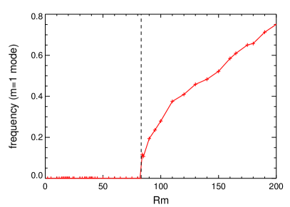
Figure 3: Growth rates (top) and frequencies (bottom) versus ${\rm{Rm}}$ for the axisymmetric flow field given by (4) and (5).

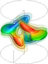
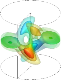
Figure 4: Magnetic field energy density $B^{2}$ for ${\rm{Rm}}=60$ (left) and ${\rm{Rm}}=120$ (right). The isosurfaces are colored with the azimuthal field.

The upper panel of Fig. 3 shows the magnetic field growth rate against the magnetic Reynolds number for the basic flow without perturbation. Due to the axisymmetry of the flow field all azimuthal modes are decoupled and follow separate curves. Regarding the $m=1$ mode (red curve in Fig. 3), we can roughly divide the solutions into two regimes. Below ${\rm{Rm}}\approx 83$ the $m=1$ mode is clearly dominant and does not oscillate. Dynamo solutions with a positive growth rate are found in the range $39\lesssim{\rm{Rm}}\lesssim 78$. Above ${\rm{Rm}}\approx 83$ the mode with $m=1$ changes its character into an oscillating mode (see bottom panel in Fig. 3) which always describes a decaying solution that does not cross the dynamo threshold. Despite the different temporal behavior, the structure of both eigenmodes is quite similar (see Fig. 4). A timeseries showing the evolution of the magnetic field at ${\rm{Rm}}=120$ is shown in Fig. 5.

Indeed, we find time-dependent solutions with the characteristic evolution shown in Fig. 5 in all our simulations with a magnetic Reynolds number above ${\rm{Rm}}=83$. These results are typical for a dynamo beyond an ”exceptional point”, which is a point in the spectrum of a linear operator where two eigenfunctions coalesce which, until this point, had different growth rates and zero frequencies (see, e.g., Refs. Kato (1976); Berry (2004)). In the present case the observed behavior can be explained only by means of two eigenfunctions with different radial structures having complex-conjugate eigenvalues with exactly (and not only approximately) the same growth rates and opposite frequencies. The appearance of such modes with complex-conjugate eigenvalues is quite common in dynamo theory. Dynamos exhibiting such exceptional points are, for example, found in simple spherically symmetric $\alpha^{2}$ dynamo models with radially varying $\alpha$ profiles, which served also as a simple model to understand reversals of the geomagnetic field Stefani and Gerbeth (2005); Stefani et al. (2006b). The typical exceptional point pattern for the formation of such modes modes is nicely visible in the red curves of Fig. 3.

II.2.2 Nonaxisymmetric perturbation

In the following we present results from simulations with the perturbation added to the basic flow at ${\rm{Rm}}=30$ where the growth rates of the firts unperturbed eigenmodes are well separated and at ${\rm{Rm}}=120$ where the growth rates of the unperturbed eigenmodes are rather close. In both cases the unperturbed solutions do not exhibit dynamo action. However, for ${\rm{Rm}}=120$ the unperturbed solutions exhibits an oscillation of the amplitude with a frequency of $|\omega_{0}|\approx 0.41$.

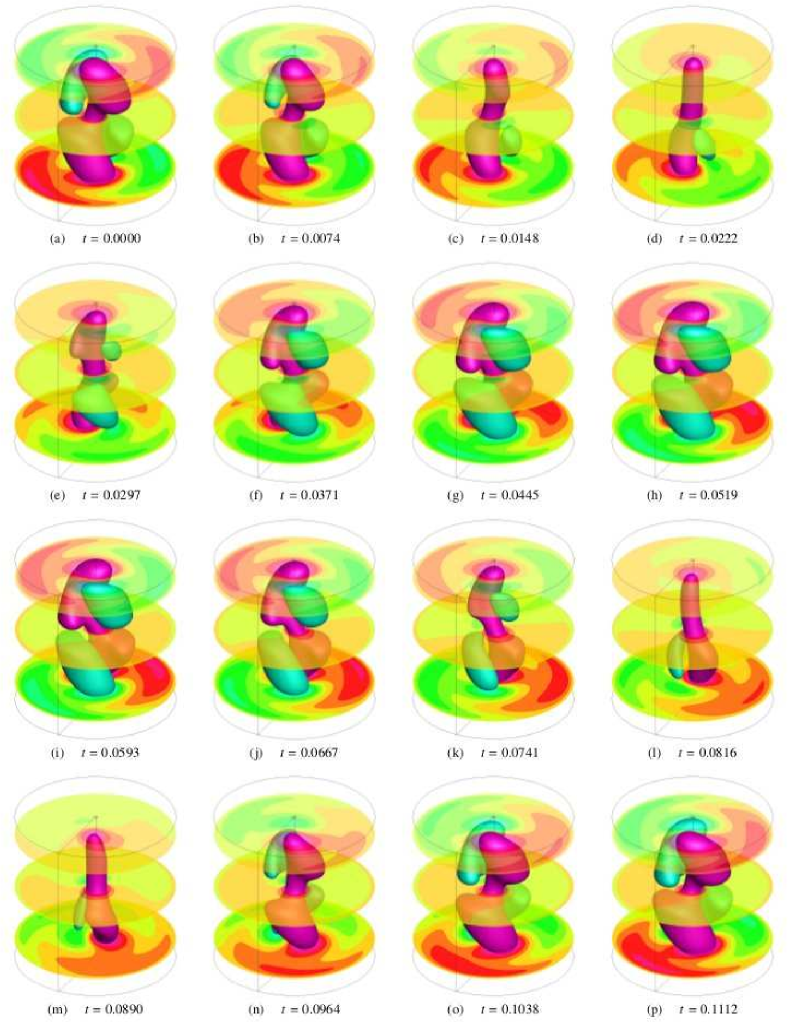
Figure 5: Evolution of the structure of the axial magnetic field component $B_{z}$ during one oscillation period. The isosurfaces show time snapshots of $B_{z}$ at $50\%$ of the time-averaged absolute value. The exponential decay has been removed. ${\rm{Rm}}=120$, unperturbed run ($\epsilon=0$).

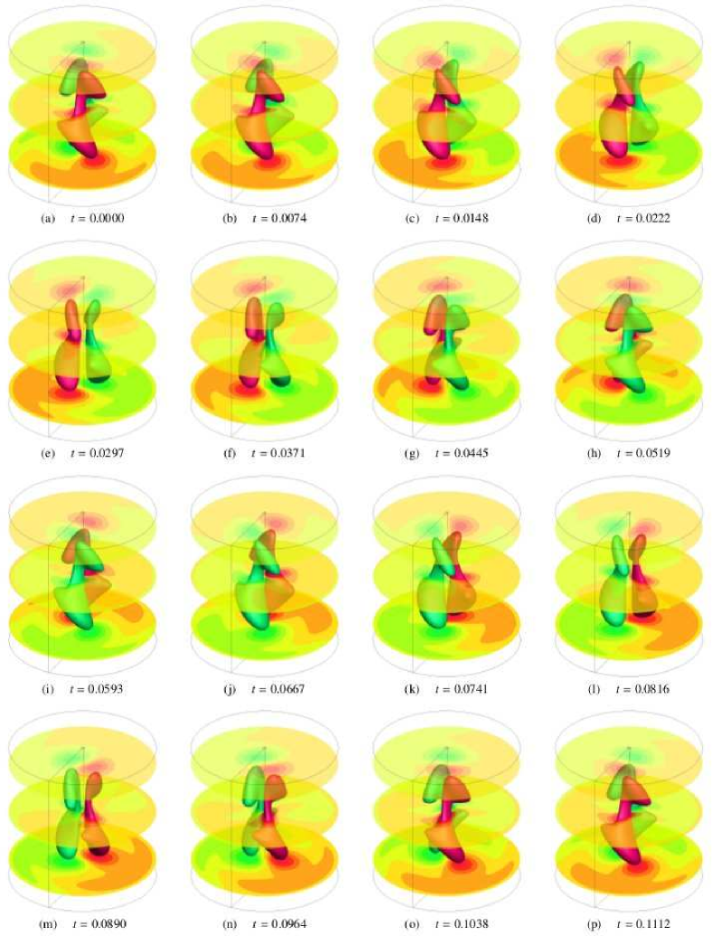
Figure 6: Evolution of the structure of the axial magnetic field component $B_{z}$ with velocity perturbation in the resonant case during one rotation period. The isosurfaces show time snapshots of $B_{z}$ at $50\%$ of the time-averaged absolute value. The exponential growth has been removed. ${\rm{Rm}}=120,\epsilon=0.3,\omega=1$.

The addition of the perturbation slightly changes the geometric structure of the eigenmodes (see Fig. 6) and has a clear impact on growth rate and/or frequency (Figs. 7 and 8). In all cases, the growth rates tend to their unperturbed values for large perturbation frequencies $|\omega|$ and we find sharp, narrow maxima symmetrically distributed around the origin. At ${\rm{Rm}}=30$ we find one maximum at $\omega=0$ [Figs. 7a and 7b] whereas at ${\rm{Re}}=120$ we find two maxima around $\omega\approx\pm 1$ with the exact location of the maxima slightly depending on the amplitude of the perturbation $\epsilon$ [Figs 7c and 7d]. In the vicinity of these maxima the growth rates show a parabolic behavior and in the following we call this regime the resonant regime [marked by the shaded regions for $\epsilon=0.3$ in Figs. 7b and 7d].

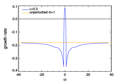
(a) $\quad{\rm{Rm}}=30,\epsilon=0.3$.

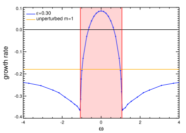
(b) Zoom on the center of (a). The shaded region denotes the regime with parametric resonance

(c) ${\rm{Rm}}=120$. The shaded red region denotes the regime with parametric amplification for $\epsilon=0.3$.

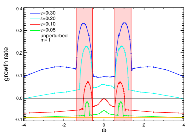
(d) Zoom on the center of (c). The shaded red region denotes the regime with parametric resonance for $\epsilon=0.3$.

Figure 7: Growth rates against the perturbation frequency for ${\rm{Rm}}=30$ [(a), (b)] and ${\rm{Rm}}=120$ [(c), (d)] for various perturbation amplitudes $\epsilon$. The right-hand side provides a detailed view of the behavior close to the origin.

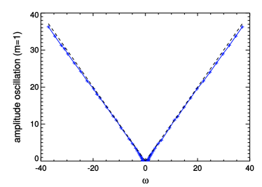
(a) ${\rm{Rm}}=30,\epsilon=0.3$

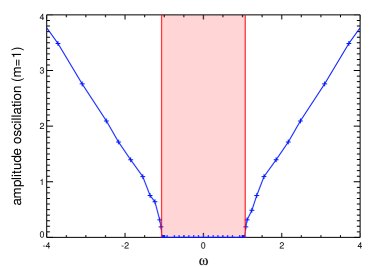
(b) Zoom on the center of (a). The red shaded region denotes the regime with parametric resonance.

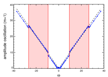
(c) ${\rm{Rm}}=120,\epsilon=0.3$. The red shaded region denotes the regime with parametric amplification that goes along with a small shift of the amplitude oscillation.

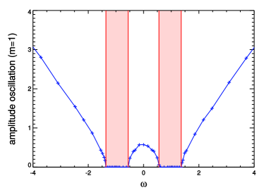
(d) Zoom on the center of (c). The red shaded region denotes the regime with parametric resonance at $\epsilon=0.3$.

Figure 8: Frequencies of the amplitude oscillations versus perturbation drift frequency for ${\rm{Rm}}=30$ [(a), (b)] and ${\rm{Rm}}=120$ [(c), (d)]. The right-hand side provides a detailed view on the behavior close to the origin.

Regarding the frequencies (Fig. 8) we see an amplitude oscillation except in the resonant regime [marked by the shaded regions in the right panels of Figs. 8b and 8d] where the amplitude oscillations vanish. In that regime the field pattern exactly follows the perturbation pattern, i.e., the magnetic field exhibits an azimuthal drift $\omega_{\rm{d}}$ that is determined by the frequency of the perturbation (phase locking, $\omega_{\rm{d}}=\omega/2$ for the $\widetilde{m}=2$ perturbation; see time series in Fig. 6). For large $|\omega|$ the azimuthal phases of magnetic field and velocity perturbation are not connected and we see an amplitude oscillation of the magnetic frield with an oscillation frequency $\omega_{\rm{a}}$ roughly proportional to the excitation frequency $\omega_{\rm{a}}\sim\omega$.

In the following, we refer to the above described resonances as parametric resonances that approximately fulfill the relation for the location of the resonance maximum $\omega_{\rm{res}}=2\omega_{0}$ with $\omega_{0}$ the eigenfrequency of the unperturbed problem which would be $\omega_{0}\approx 0.41$ for the case shown in Figs. 8c and 8d. The deviation from this relation increases for increasing $\epsilon$, most probably because of the growing impact of the perturbation on the base state. A dependence of the location of the maxima on the parameter $\epsilon$ is also observed in our model introduced in Sec. III (see Sec. III.3.3 and Fig. 15).

For weak amplitudes of the perturbation we see a weakly pronounced third maximum between the main maxima [e.g., see red curve for $\epsilon=0.1$ in Figs 7c and 7d]. Similar to the solution shown in Fig. 14 below this interim maximum is not connected to a regime with phase locking and vanishes for increasing $\epsilon$.

At ${\rm{Rm}}=30$ we find no further features beside the parametric resonances in the behavior of the growth rates. This can be attributed to the large differences of the unperturbed growth rates (see Fig. 3, top panel) of the distinct azimuthal eigenmodes which reduces the interaction between the individual modes. The behavior changes at ${\rm{Rm}}=120$ where, in addition to the sharp resonance peak, a number of further extremes emerge at larger $|\omega|$ with a rather broad shape. These maxima do not occur in conjunction with phase locking, and the enhancement of dynamo action is less intense than within the regime of parametric resonance. In the following, we refer to this phenomenon as a parametric amplification to distinguish from the mere parametric resonance. In the amplification regime, the frequency of the amplitude oscillation varies roughly $\propto\omega$ with a small jump within the outer maxima ([ee Fig. 8c]. This jump indicates that in this regime a different eigenmode dominates compared to the mode around the origin (with the parametric resonance).

The nearly perfect symmetry with respect to the origin differs from the behavior found in a previous study Giesecke et al. (2012a) where an imposed breaking of the equatorial symmetry of the flow causes a faster azimuthal drift of the leading dynamo mode proportional to the degree of symmetry breaking and a corresponding asymmetric behavior of the resonance maximum with respect to the origin.

The boost of growth rates seen in Fig. 7 is also reflected in the behavior of the critical magnetic Reynolds number ${\rm{Rm}}^{\rm{crit}}$ that is required for the onset of dynamo action. There are considerable variations of the growth rates with ${\rm{Rm}}$ and with $\omega$ (see Fig. 9). However, when restricting ${\rm{Rm}}$ to the crucial regime in the vicinity of the dynamo threshold, the growth rates do not change much with the perturbation frequency, and nearly all curves around the onset of dynamo action take the same evolution (Fig. 9). A beneficial impact on dynamo action is found only for small $\omega$ (blue curves in Fig. 9). Accordingly, the most significant decrease in ${\rm{Rm}}^{\rm{crit}}$ is found for $\omega=0$ [Fig. 10a], and the reduction can reach considerable values of up to $30\%$ [from ${\rm{Rm}}^{\rm{crit}}=39.6$ at $\epsilon=0$ to ${\rm{Rm}}^{\rm{crit}}=26.3$ at $\epsilon=0.5$, Fig. 10b].

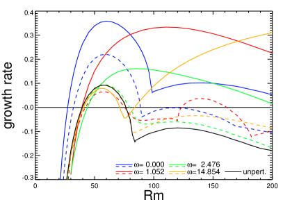
Figure 9: Growth rate versus ${\rm{Rm}}$ for $\epsilon=0.1$ (dashed curves) and $\epsilon=0.3$ (solid curves). The solid black curve denotes the case $\epsilon=0$.

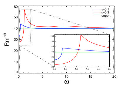
(a)

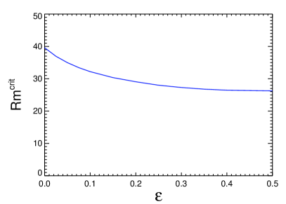
(b)

Figure 10: (a) Critical magnetic Reynolds numbers against perturbation frequency $\omega$ for $\epsilon=0.1$ and $\epsilon=0.3$. The horizontal green line denotes the case $\epsilon=0$. (b) Critical magnetic Reynolds number versus perturbation amplitude $\epsilon$ for $\omega=0$ where the maximum reduction of ${\rm{Rm}}^{\rm{crit}}$ takes place.

The behavior of ${\rm{Rm}}^{\rm{crit}}$ with the sharp reduction around $\omega\approx 0$ essentially reflects the structure of the growth rates at ${\rm{Rm}}=30$ with one sharp peak around $\omega=0$ as is shown in Figs. 7a and 7b. The secondary regimes with enhanced growth rates that emerge at larger Reynolds number and larger perturbation frequencies hardly impact the primary onset of dynamo action around ${\rm{Rm}}\approx 30\dots 40$ but can be related to a second dynamo regime with a threshold around ${\rm{Rm}}\approx 120$ (see, e.g., solid red curve in Fig. 9) where no dynamo action is obtained at all without perturbation. The existence of a second regime with dynamo action is less important in the context of experimental dynamos but can be associated with subcritical phenomena in fully nonlinear simulations and may be causative for possible deviations from ideal scaling laws by providing additional energy for the dynamo process Le Bars et al. (2015).

III Low-dimensional model

III.1 Amplitude equation

In order to find a qualitative explanation for the behavior observed in the simulations presented above, we derive a simple low-dimensional analytical model for the amplitude of distinct dynamo modes. The framework presented in this section must be seen as a toy model, where the parameters are chosen to reproduce qualitatively the observed features in the former section. Our model is based on an azimuthal decomposition of the global magnetic field. In doing so, the dynamics of each azimuthal mode is determined by one eigenmode with the largest growth rate. The decomposition yields a linear system of equations that couples all odd azimuthal wave numbers. From this model, we find different scenarios leading to an enhancement of the growth rate, which are not described by the classical parametric instability. Although we assume a cylindrical domain, most of the following considerations require only the existence of a well-defined symmetry axis in order to allow a reasonable decomposition into azimuthal field modes and are also valid, e.g., in spherical geometry.

We start again with the magnetic induction equation (8). We assume a prescribed velocity field $\mbox{\boldmath$U$}=\mbox{\boldmath$U$}(\mbox{\boldmath$r$},t)$ that is composed of an axisymmetric component $\mbox{\boldmath$U$}_{0}$ and a periodic perturbation with the azimuthal wave number $\widetilde{m}$ propagating in the azimuthal direction with the frequency $\omega$:

$$\!\!\!\mbox{\boldmath$U$}(\mbox{\boldmath$r$},t)\!=\!\mbox{\boldmath$U$}_{0}(r,z)\!+\!\epsilon\left[\mbox{\boldmath$u$}_{\widetilde{m}}(r,z)e^{i({\widetilde{m}}\varphi+\omega t)}\!+\mbox{\boldmath$u$}_{-{\widetilde{m}}}(r,z)e^{-i({\widetilde{m}}\varphi+\omega t)}\right],$$ (10)

where the parameter $\epsilon$ characterizes the amplitude of the perturbation. We now reduce the induction equation to a system of equations for the amplitudes of azimuthal magnetic field modes characterized by a wave number $m$. We assume that the magnetic field $B$ can be decomposed according to

$$\mbox{\boldmath$B$}=\sum\limits_{-M}^{M}\hat{b}_{m}^{\mbox{}}(t)\mbox{\boldmath$b$}_{m}(r,z)e^{im\varphi}$$ (11)

with the complex amplitude $\hat{b}_{m}(t)\in\mathbb{C}$ that fulfills $\hat{b}_{m}=\hat{b}_{-m}^{*}$ in order to ensure a real valued magnetic field. We further suppose a normalization for the function $\mbox{\boldmath$b$}_{m}$ given by

$$\iint\mbox{\boldmath$b$}_{m}^{\mbox{ }}\cdot\mbox{\boldmath$b$}_{m}^{*}rdrdz=1.$$ (12)

The decomposition (11) assumes that the individual modes are modulated only by a simple temporal varying amplitude which in general is not correct (if the linear operator is nonnormal as in case of the induction equation). Furthermore, we consider only the leading eigenmode for each azimuthal wave number, and we additionally suppose that only one single mode is close to be unstable. Consequently, the decomposition (11) into azimuthal modes can at least qualitatively be justified.

The coefficient $\hat{b}_{m}(t)$ can be computed by forming the scalar product

$$\hat{b}_{m}(t)=\big{<}\mbox{\boldmath$B$},\mbox{\boldmath$b$}_{m}\big{>}=\iiint\mbox{\boldmath$B$}\cdot\mbox{\boldmath$b$}^{*}_{m}e^{-im\varphi}dV$$ (13)

so that the temporal evolution of $\hat{b}_{m}(t)$ is governed by

$$\frac{d}{dt}\hat{b}_{m}(t)=\frac{d}{dt}\bigg{<}\mbox{\boldmath$B$},\mbox{\boldmath$b$}_{m}\bigg{>}=\bigg{<}\nabla\times\big{(}\mbox{\boldmath$U$}\times\mbox{\boldmath$B$}\big{)}+\eta\Delta\mbox{\boldmath$B$},\mbox{\boldmath$b$}_{m}\bigg{>}.$$ (14)

Using the velocity field (10) with an explicit $\widetilde{m}=2$ distortion yields the evolution equation for the amplitude $\hat{b}_{m}(t)$ with an explicit coupling to the magnetic modes $\hat{b}_{m\pm 2}(t)$:

$$\frac{d}{dt}\hat{b}_{m}(t)=\alpha_{{m},{m}}\hat{b}_{m}+\epsilon\left(e^{-i\omega t}\alpha_{{m},{m}+2}\hat{b}_{m+2}+e^{i\omega t}\alpha_{{m},{m}-2}\hat{b}_{m-2}\right)$$ (15)

with

$$\alpha_{{m},{m}} \!=\! \!\iiint\!\!\bigg{(}\nabla\!\!\times\!\big{(}\mbox{\boldmath$U$}_{0}\!\times\!\mbox{\boldmath$b$}_{m}e^{im\varphi}\big{)}\!+\!\eta\Delta\mbox{\boldmath$b$}_{m}e^{im\varphi}\!\bigg{)}\!\cdot\!\mbox{\boldmath$b$}_{m}^{*}e^{-im\varphi}dV,$$

$$\alpha_{{m},{m}\pm 2} \!=\! \!\iiint\!\!\bigg{(}\nabla\!\times\!\big{(}\mbox{\boldmath$u$}_{\mp 2}\times\mbox{\boldmath$b$}_{m\pm 2}e^{im\varphi}\big{)}\bigg{)}\cdot\mbox{\boldmath$b$}^{*}_{m}e^{-im\varphi}dV.$$

The magnetic field $B$ must be a real valued function which requires $\hat{b}_{m}=\hat{b}_{-m}^{*}$ and hence entails

$$\alpha_{{m},{m}}=\alpha^{*}_{-{m},-{m}}\mbox{ and }\alpha_{{m},{m}\pm 2}=\alpha^{*}_{-{m},-{m}\mp 2}.$$ (17)

We now write system (15) in an explicit form

$$\begin{array}[]{lclclcl}&\vdots&&&&\\ \displaystyle\frac{d}{dt}\hat{b}_{-5}\!\!&\!\!=\!\!&\!\epsilon e^{i\omega t}\alpha_{-5,-7}\hat{b}_{-7}\!\!&\!+\!&\!\!\alpha_{-5,-5}\hat{b}_{-5}\!\!&\!+\!&\!\!\epsilon e^{-i\omega t}\alpha_{-5,-3}\hat{b}_{-3},\\[7.11317pt] \displaystyle\frac{d}{dt}\hat{b}_{-3}\!\!&\!\!=\!\!&\!\epsilon e^{i\omega t}\alpha_{-3,-5}\hat{b}_{-5}\!\!&\!+\!&\!\!\alpha_{-3,-3}\hat{b}_{-3}\!\!&\!+\!&\!\!\epsilon e^{-i\omega t}\alpha_{-3,-1}\hat{b}_{-1},\\[7.11317pt] \displaystyle\frac{d}{dt}\hat{b}_{-1}\!\!&\!\!=\!\!&\!\epsilon e^{i\omega t}\alpha_{-1,-3}\hat{b}_{-3}\!\!&\!+\!&\!\!\alpha_{-1,-1}\hat{b}_{-1}\!\!&\!+\!&\!\!\epsilon e^{-i\omega t}\alpha_{-1,1}\hat{b}_{1},\\[7.11317pt] \displaystyle\frac{d}{dt}\hat{b}_{1}\!\!&\!\!=\!\!&\!\epsilon e^{i\omega t}\alpha_{1,-1}\hat{b}_{-1}\!\!&\!+\!&\!\!\alpha_{1,1}\hat{b}_{1}\!\!&\!+\!&\!\!\epsilon e^{-i\omega t}\alpha_{1,3}\hat{b}_{3},\\[7.11317pt] \displaystyle\frac{d}{dt}\hat{b}_{3}\!\!&\!\!=\!\!&\!\epsilon e^{i\omega t}\alpha_{3,1}\hat{b}_{1}\!\!&\!+\!&\!\!\alpha_{3,3}\hat{b}_{3}\!\!&\!+\!&\!\!\epsilon e^{-i\omega t}\alpha_{3,5}\hat{b}_{5},\\[7.11317pt] \displaystyle\frac{d}{dt}\hat{b}_{5}\!\!&\!\!=\!\!&\!\epsilon e^{i\omega t}\alpha_{5,3}\hat{b}_{3\!\!}&\!+\!&\!\!\alpha_{5,5}\hat{b}_{5}\!\!&\!+\!&\!\!\epsilon e^{-i\omega t}\alpha_{5,7}\hat{b}_{7},\\[7.11317pt] &\vdots&&&&\\ \end{array}$$ (26)

which can be written in compact form as a matrix equation

$$\frac{d}{dt}{B}(t)=A(t)B(t)$$ (27)

with $B(t)=(\cdots,\hat{b}_{-m},\hat{b}_{-m+2},\dots,\hat{b}_{-1},\hat{b}_{1},\dots,\hat{b}_{m-2},\hat{b}_{m}\cdots)^{T}$ and a tridiagonal matrix $A(t)$ given by

$$A=\left(\begin{array}[]{cccccccccc}&&\ddots&&&&&&&\\ \cdots&0&\delta_{3}^{*}f^{*}_{t}&\alpha_{3}^{*}&\delta_{2}^{*}f_{t}&0&\cdots&&&\\ &\cdots&0&\delta_{1}^{*}f^{*}_{t}&\alpha_{1}^{*}&\gamma^{*}f_{t}&0&\cdots&&\\ &&\cdots&0&\gamma f^{*}_{t}&\alpha_{1}&\delta_{1}f_{t}&0&\cdots&\\ &&&\cdots&0&\delta_{2}f^{*}_{t}&\alpha_{3}&\delta_{3}f_{t}&0&\cdots\\ &&&&&&&\ddots&&\\ \end{array}\right),$$ (28)

where we used the abbreviations $\alpha_{j}=\alpha_{j,j}$, $\gamma=\alpha_{1,-1}$, $\delta_{1}=\alpha_{1,3}$, $\delta_{2}=\alpha_{3,1}$, $\delta_{3}=\alpha_{3,5}$ and $f_{t}=\epsilon e^{-i\omega t}$. The nondiagonal elements of $A$ represent the coupling between the azimuthal modes introduced by the nonaxisymmetric flow perturbation. In the unperturbed case these nondiagonal elements vanish and all azimuthal modes $\hat{b}_{m}(t)$ decouple. In that case the diagonal elements are the eigenvalues

$$\alpha_{j,j}=\alpha_{j}=\alpha_{j}^{r}+i\alpha_{j}^{i},$$

where $\alpha^{r}_{j}$, the real part of $\alpha_{j}$, denotes the growth rate of the unperturbed case and implicitly incorporates the magnetic Reynolds number, and $\alpha^{i}_{j}$, the imaginary part of $\alpha_{j}$, denotes the frequency of the unperturbed case. The off-diagonal parameters, originally labeled with $\alpha_{m,m\pm 2}$, prescribe the interaction of the modes with themselves and/or with adjacent modes.

In case of a perturbation with an azimuthal wave number $\widetilde{m}=2$ we achieve two classes of magnetic modes which incorporate even azimuthal wave numbers and odd azimuthal wave numbers. Here only the second class with odd wave numbers is relevant because the even modes typically decay on a faster time scale, and we could not find any growing solutions with even azimuthal symmetry in our simulations presented above.

Note that the approach outlined above does not constitute a perturbation theory in the strict mathematical sense. The nonaxisymmetric spatio-temporally periodic perturbation changes the structure of the solution (the geometry of the eigenvector) by coupling different azimuthal modes, and the limiting case $\epsilon\rightarrow 0$ is different from the case $\epsilon=0$. This means that the addition of a propagating wave with $\epsilon\neq 0$ changes the shape of the modes $\mbox{\boldmath$b$}_{m}$ in comparison with the simple axisymmetric case so that the coefficients $\alpha_{m,m}$ depend implicitly on $\epsilon$ and $\omega$. However, in the limit $\epsilon\rightarrow 0$ we assume that $\alpha_{m,m}(\epsilon\neq 0)\approx\alpha_{m,m}(\epsilon=0)$ and that the addition of a nonaxisymmetric perturbation does not change the eigenvector of the unperturbed problem.

III.2 Direct solution for truncation at $m=\pm 1$

In order to solve the set of ordinary differential equations for the eigenvalues, i.e., growth rate and frequency, the system must be truncated at a fixed azimuthal wave number $M$. We start with the most severe approximation and cut the system (26) at $m=\pm 1$. We obtain two coupled differential equations

$$\frac{d\hat{b}_{-1}}{dt} = \alpha^{*}\hat{b}_{-1}+\epsilon\gamma^{*}e^{-i\omega t}\hat{b}_{1},$$ (29)

$$\frac{d\hat{b}_{1}}{dt} = \epsilon\gamma e^{i\omega t}\hat{b}_{-1}+\alpha\hat{b}_{1},$$ (30)

where we used the abbreviations

$$\begin{array}[]{rcccl}\alpha&=&\alpha_{1,1}&=&\alpha^{*}_{-1,-1},\\ \gamma&=&\alpha_{1,-1}&=&\alpha^{*}_{-1,1}.\end{array}$$ (31)

Taking the derivative of Eq. (30) yields

$$\frac{d^{2}\hat{b}_{1}}{dt^{2}}=\epsilon\gamma e^{i\omega t}\left(i\omega\hat{b}_{-1}+\frac{d\hat{b}_{-1}}{dt}\right)+\alpha\frac{d\hat{b}_{1}}{dt}.$$ (32)

We use (29) to replace $\displaystyle\frac{d\hat{b}_{-1}}{dt}$ and then (30) to ultimately get rid off $\hat{b}_{-1}$ which gives

$$\frac{d^{2}\hat{b}_{1}}{dt^{2}} = \left[-i\omega\alpha-|\alpha|^{2}+\epsilon^{2}|\gamma|^{2}\right]\hat{b}_{1}+\left(i\omega+2{\alpha_{r}}\right)\frac{d\hat{b}_{1}}{dt}.$$ (33)

We search for solutions $\hat{b}_{1}(t)\propto e^{\sigma t}$ which yields the relation

$$\sigma^{2}-\left(i\omega+2{\alpha_{r}}\right)\sigma-\left[-i\omega\alpha-|\alpha|^{2}+\epsilon^{2}|\gamma|^{2}\right]=0$$ (34)

with the solutions

$$\sigma_{1,2}={\alpha^{r}}+i\frac{\omega}{2}\pm\frac{1}{2}\sqrt{4\epsilon^{2}|\gamma|^{2}-\left({2\alpha^{i}-\omega}\right)^{2}}.$$ (35)

We distinguish two cases in dependence of the sign of $4\epsilon^{2}|\gamma|^{2}-(2\alpha^{i}-\omega)^{2}$.

(1) For $\displaystyle|2\alpha^{i}-{\omega}|<2\epsilon|\gamma|$ we obtain one frequency

$$\sigma^{i}=\displaystyle\frac{\omega}{2}$$ (36)

and two different growth rates

$$\sigma^{r}_{1,2}=\alpha^{r}\pm\frac{1}{2}\sqrt{4\epsilon^{2}|\gamma|^{2}-\left(2\alpha^{i}-\omega\right)^{2}}.$$ (37)

For small deviations of the forcing frequency ${\omega}$ from twice the unperturbed frequency $2\alpha^{i}$ we can write for the growth rate:

$$\sigma^{r}_{1,2}\approx\alpha^{r}\pm\epsilon|\gamma|\left(1-\frac{(2\alpha^{i}-\omega)^{2}}{4\epsilon^{2}|\gamma|^{2}}\right),$$ (38)

and we find two extrema for the growth rate $\sigma^{r,{\rm{max}}}_{1,2}=\alpha^{r}\pm\epsilon|\gamma|$ when the perturbation frequency is equal to twice the intrinsic frequency $\omega=2\alpha^{i}$. Around this maximum the growth rate is locally parabolic.

(2) For $\displaystyle|2\alpha^{i}-\omega|>2\epsilon|\gamma|$ we get only one growth rate

$$\sigma^{r}=\alpha^{r}$$ (39)

and two frequencies

$$\sigma^{i}_{1,2}=\frac{\omega}{2}\pm\frac{1}{2}\sqrt{\left(2\alpha^{i}-\omega\right)^{2}-4\epsilon^{2}|\gamma|^{2}}.$$ (40)

For large $\omega$ these frequencies tend to $\sigma^{i}_{1}=\omega$ and $\sigma^{i}_{2}=\alpha^{i}$.

Figure 11 shows the behavior of $\sigma$ (top panel: growth rate, bottom panel: frequency) versus the perturbation frequency.

Figure 11: Growth rate (top) and frequency (bottom) versus ${\omega}$ for $\alpha^{r}=0$, $\alpha^{i}=0$, $|\gamma|^{2}=1$, and $\epsilon=0.3$. The solid (dashed) curve shows the solution corresponding to ${\sigma}_{1}({\sigma}_{2})$.

In the resonant regime, i.e., for $\displaystyle\left|2\alpha^{i}-{\omega}\right|<2\epsilon|\gamma|$, the growth rates of both interacting modes separate and form a bubble-like pattern, and the location of the maximum is given by twice the frequency of the unperturbed problem. Width and height of the resonance are determined by the interaction parameter $\gamma$ and by the amplitude of the perturbation $\epsilon$ (height $\sim\epsilon|\gamma|$ and width $\sim 4\epsilon|\gamma|$).

In the resonant regime, we find the frequency exactly proportional to ${\omega}/{2}$, which implies that the phase of the $m=1$ eigenmode becomes locked to the $m=2$ velocity perturbation and the pattern of the nonaxisymmetric magnetic field is enslaved to the azimuthal phase of the flow perturbation. Outside of the resonant regime, i.e., for $\displaystyle\left|2\alpha^{i}-{\omega}\right|>2\epsilon|\gamma|$ the growth rates collapse, and we find two frequencies with different asymptotic behavior for $|\omega|\gg 1$. One solution converges against the unperturbed value, $\alpha^{i}$ (Fig. 11, solid curve in bottom panel), and the second solution tends to the frequency of the perturbation $\omega$ (Fig. 11, dashed curve in bottom panel).

Two distinguished locations can be found exactly at the transition from the nonresonant to the resonant regime. At these exceptional points Kato (1976); Berry (2004), where $|\omega-2\alpha^{i}|=\pm 2\epsilon|\gamma|$, we see an abrupt change of growth rates and frequencies in combination with a degeneration of the eigenvalues and a collapse of the corresponding eigenfunctions.

III.3 Coupling to larger azimuthal wave numbers

III.3.1 Application of Floquet theory

We now treat the general case and consider system (26) for in principle arbitrary $m$ anticipating that later we will have to truncate our model at a fixed value for $m_{\rm{max}}=\pm M$ in order to perform explicit calculations of the eigenvalues. We revert to Floquet theory (see, e.g., Rewf. Coddington and Carlson (1997)), which implies that the time dependence of the solution of a differential equation of the form

$$\frac{d}{dt}B(t)=A(t)B(t)$$ (41)

with a $T$-periodic matrix $A(t)=A(t+T)$ and a $n-$dimensional vector $B$ is given by

$$B(t)=P(t)e^{Rt}$$ (42)

with a $T$-periodic invertible matrix $P(t)=P(t+T)$ and a constant matrix $R$. It is always possible to find a transformation, the Lyapunov-Floquet transformation,

$$B(t)=P(t)X(t),$$ (43)

such that the previously time dependent linear system (41) becomes a linear system

$$\frac{d}{dt}X(t)=RX(t)$$ (44)

with the time-independent coefficient matrix $R$. From (41) and (42) we get

$$\frac{d}{dt}B=\dot{P}e^{Rt}+PRe^{Rt}=APe^{Rt}$$ (45)

so that

$$R=P^{-1}AP-P^{-1}\dot{P}.$$ (46)

We now write

$$P=e^{iDt}$$ (47)

from which immediately follows

$$P^{-1}\dot{P}=iD$$ (48)

so that the constant coefficient matrix $R$ in the transformed system (44) can be written as

$$R=e^{-iDt}Ae^{iDt}-iD.$$ (49)

In our particular case we can write

$$A(t)=\displaystyle e^{iD_{\omega}t}\hat{A}e^{-iD_{\omega}t}$$ (50)

with

$$D_{\omega}=\left(\begin{array}[]{ccccc}-\frac{M}{2}\omega&0&&&\\ 0&-\frac{M-2}{2}\omega&0&&\\ &0&\ddots&0&\\ &&0&\frac{M-2}{2}\omega&0\\ &&&0&\frac{M}{2}\omega\end{array}\right)$$ (51)

and $\hat{A}$ the matrix with the components of $A$ but without the time modulation $e^{\pm i\omega t}$. This gives

$$R=\hat{A}-iD_{\omega}$$ (52)

so that from (44) we end up with the system

$$\frac{dX}{dt}=\left(\hat{A}-iD_{\omega}\right)X.$$ (53)

The solutions are given by $X=X_{0}e^{\widetilde{\sigma}t}$ with $\widetilde{\sigma}\in\mathbb{C}$ the eigenvalues in the transformed system which are the roots of the characteristic equation

$$\left|\hat{A}-iD_{\omega}-\widetilde{\sigma}\mathbb{I}\right|=0,$$ (54)

where $|\cdots|$ denotes the determinant and $\mathbb{I}$ is the identity matrix.

III.3.2 Truncation at $M=1$

In order to check the validity of the computations from the previous section we solve the case $M=1$ and compare with the solution obtained in Sec. III.2. We have

$$\left(\begin{array}[]{l}\displaystyle\frac{d}{dt}\hat{b}_{-1}\\[9.95863pt] \displaystyle\frac{d}{dt}\hat{b}_{1}\end{array}\right)=\left(\begin{array}[]{cc}\vphantom{\displaystyle\frac{d}{dt}}\alpha^{*}&\epsilon e^{-i\omega t}\gamma^{*}\\[9.95863pt] \vphantom{\displaystyle\frac{d}{dt}}\epsilon e^{i\omega t}\gamma&\alpha\end{array}\right)\left(\begin{array}[]{c}\vphantom{\displaystyle\frac{d}{dt}}\hat{b}_{-1}\\[9.95863pt] \vphantom{\displaystyle\frac{d}{dt}}\hat{b}_{1}\end{array}\right)=\left(\begin{array}[]{cc}\vphantom{\displaystyle\frac{d}{dt}}e^{-i\frac{\omega}{2}t}&0\\[9.95863pt] \vphantom{\displaystyle\frac{d}{dt}}0&e^{i\frac{\omega}{2}t}\end{array}\right)\left(\begin{array}[]{cc}\vphantom{\displaystyle\frac{d}{dt}}\alpha^{*}&\epsilon\gamma^{*}\\[9.95863pt] \vphantom{\displaystyle\frac{d}{dt}}\epsilon\gamma&\alpha\end{array}\right)\left(\begin{array}[]{cc}\vphantom{\displaystyle\frac{d}{dt}}e^{i\frac{\omega}{2}t}&0\\[9.95863pt] \vphantom{\displaystyle\frac{d}{dt}}0&e^{-i\frac{\omega}{2}t}\end{array}\right)\left(\begin{array}[]{l}\vphantom{\displaystyle\frac{d}{dt}}\hat{b}_{-1}\\[9.95863pt] \vphantom{\displaystyle\frac{d}{dt}}\hat{b}_{1}\end{array}\right)$$ (55)

so that

$$\hat{A}=\left(\begin{array}[]{cc}\alpha^{*}&\epsilon\gamma^{*}\\ \epsilon\gamma&\alpha\end{array}\right)\mbox{ and }D_{\omega}=\left(\begin{array}[]{cc}\nicefrac{{-\omega}}{{2}}&0\\ 0&\nicefrac{{\omega}}{{2}}\end{array}\right).$$ (60)

The characteristic equation for the eigenvalues becomes

$$\left(\alpha^{*}+i\frac{\omega}{2}-\widetilde{\sigma}\right)\left(\alpha-i\frac{\omega}{2}-\widetilde{\sigma}\right)-\epsilon^{2}\left|\gamma\right|^{2}=0$$ (61)

with the solutions

$$\widetilde{\sigma}_{1,2}=\alpha^{r}\pm\frac{1}{2}\sqrt{4\epsilon^{2}|\gamma|^{2}-\left(2\alpha^{i}-\omega\right)^{2}},$$ (62)

which, when taking into account the transformation $B=P(t)X(t)=e^{iD_{\omega}t}X$ according to Eq. (43), is identical to the solution (35) obtained previously in Sec. III.2.

III.3.3 Truncation at $M=3$

In the next step we include higher order modes with $m=\pm 3$ so that we have to compute the characteristic equation

$$\left|\begin{array}[]{cccc}\alpha^{*}_{3}\!+\!i\frac{3\omega}{2}\!-\!\widetilde{\sigma}\!&\epsilon\delta^{*}_{2}&0&0\\ \epsilon\delta^{*}_{1}&\alpha_{1}^{*}\!+\!i\frac{\omega}{2}\!-\!\widetilde{\sigma}\!&\epsilon\gamma^{*}&0\\ 0&\epsilon\gamma&\alpha_{1}\!-\!i\frac{\omega}{2}\!-\!\widetilde{\sigma}\!&\epsilon\delta_{1}\\ 0&0&\epsilon\delta_{2}&\alpha_{3}\!-\!i\frac{3\omega}{2}\!-\!\widetilde{\sigma}\!\end{array}\right|=0,$$ (63)

where we used the abbreviations $\alpha_{1}=\alpha_{1,1},\alpha_{3}=\alpha_{3,3},\gamma=\alpha_{1,-1},\delta_{1}=\alpha_{1,3}$ and $\delta_{2}=\alpha_{3,1}$. Before we specify the general solution of (63) we briefly discuss three limit cases in order to prove the validity of the solution and illustrate distinct properties of the solutions resulting from different types of coupling.

Weak coupling

We first assume no coupling between $m=1$ and $m=3$ as well as between $m=+1$ and $m=-1$ (i.e., $|\gamma|^{2}=|\delta_{1}\delta_{2}|=0$) so that the matrix $A(t)$ is a diagonal matrix. We obtain the unperturbed solutions for the $m=1$ mode and a second set for the $m=3$ mode,

$$\widetilde{\sigma}_{1,2}=\alpha_{1}^{r}\pm i\left(\alpha_{1}^{i}-\frac{\omega}{2}\right)\mbox{ and }\widetilde{\sigma}_{3,4}=\alpha_{3}^{r}\pm i\left(\alpha_{3}^{i}-\frac{3\omega}{2}\right).$$ (64)

If only the coupling between the $m=\pm 1$ mode and $m=\pm 3$ is weak (i.e., $|\gamma|^{2}\gg|\delta_{1}\delta_{2}|$), we obtain the characteristic equation

$$\Bigg{[}\bigg{(}\alpha_{3}^{*}+i\frac{3\omega}{2}-\widetilde{\sigma}\bigg{)}\bigg{(}\alpha_{3}-i\frac{3\omega}{2}-\widetilde{\sigma}\bigg{)}\Bigg{]}\Bigg{[}\bigg{(}\alpha_{1}^{*}+i\frac{\omega}{2}-\widetilde{\sigma}\bigg{)}\bigg{(}\alpha_{1}-i\frac{\omega}{2}-\widetilde{\sigma}\bigg{)}-\epsilon^{2}|\gamma|^{2}\Bigg{]}=0,$$ (65)

and we recover the previous solution (35) from section III.2 with the resonance from the interaction of $m=1$ and $m=-1$ at $\omega=2\alpha_{1}^{i}$ and two separate solutions for the $m=3$ mode:

$$\widetilde{\sigma}_{1,2}=\alpha_{1}^{r}+i\frac{\omega}{2}\pm\frac{1}{2}\sqrt{4\epsilon^{2}|\gamma|^{2}-\left(\omega-2\alpha_{1}^{i}\right)^{2}}\mbox{ and }\widetilde{\sigma}_{3,4}=\alpha_{3}^{r}\pm i\left(\alpha_{3}^{i}-\frac{3\omega}{2}\right).$$ (66)

Note that the first part of Eq. (66) also corresponds to the solution denoted in Eq. (62) for a truncation at $M=1$.

Strong coupling between $m=1$ and $m=3$

Now we assume that the coupling between $m=1$ and $m=-1$ can be neglected but the coupling between $m=1$ and $m=3$ remains strong, i.e., $|\delta_{1}\delta_{2}|\gg|\gamma|^{2}$.

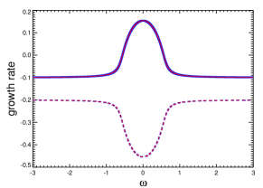
(a) Growth rate

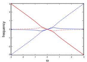
(b) Frequency

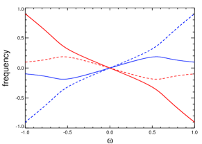
(c) Frequency (close up)

Figure 12: Growth rate (real part of $\widetilde{\sigma}_{1}\dots\\ widetilde{sigma}_{4}$) and frequencies (imaginary part of $\widetilde{\sigma}_{1}\dots\widetilde{\sigma}_{4}$) versus $\omega$ for strong coupling between $m=1$ and $m=3$ ($|\delta_{1}\delta_{2}|\gg|\gamma|^{2}$). $\alpha^{r}_{1}=-0.1,\alpha_{3}^{r}=-0.2,\alpha_{1}^{i}=\alpha_{3}^{i}=0,|\gamma|^{2}=0,\delta_{1}\delta_{2}=1,\epsilon=0.3$. The blue curves show the solutions $\widetilde{\sigma}_{1}$ (solid curves) and $\widetilde{\sigma}_{2}$ (dashed curves), and the red curves show $\widetilde{\sigma}_{3}$ (solid curves) and $\widetilde{\sigma}_{4}$ (dashed curves). Note that the real parts of $\widetilde{\sigma}_{1}$ and $\widetilde{\sigma}_{3}$ (solid curves in a) and of $\widetilde{\sigma}_{2}$ and $\widetilde{\sigma}_{4}$ (dashed curves in a) collapse exactly.

Then the characteristic equation for the calculation of the eigenvalues reads

$$\Bigg{[}\left(\alpha_{3}^{*}+i\frac{3\omega}{2}-\widetilde{\sigma}\right)\Bigg{(}\alpha_{1}^{*}+i\frac{\omega}{2}-\widetilde{\sigma}\Bigg{)}-\epsilon^{2}\delta_{1}^{*}\delta_{2}^{*}\Bigg{]}\Bigg{[}\left(\alpha_{3}-i\frac{3\omega}{2}-\widetilde{\sigma}\right)\Bigg{(}\alpha_{1}-i\frac{\omega}{2}-\widetilde{\sigma}\Bigg{)}-\epsilon^{2}\delta_{1}\delta_{2}\Bigg{]}=0.$$ (67)

and we have two kinds of solutions, one for the coupled system of $m=-1$ and $m=-3$ and a second one for the coupled system with $m=1$ and $m=3$ mode:

$$\widetilde{\sigma}_{1,2}=\quad\frac{1}{2}\bigg{[}\alpha_{1}^{r}+\alpha_{3}^{r}+i\Big{(}\alpha_{1}^{i}+\alpha_{3}^{i}-2\omega\Big{)}\bigg{]}\pm\frac{1}{2}\sqrt{4\epsilon^{2}\delta_{1}\delta_{2}+\bigg{[}\alpha_{1}^{r}-\alpha_{3}^{r}+i\Big{(}\alpha_{1}^{i}-\alpha_{3}^{i}+\omega\Big{)}\bigg{]}^{2}},$$ (68)

$$\widetilde{\sigma}_{3,4}=\quad\frac{1}{2}\bigg{[}\alpha_{1}^{r}+\alpha_{3}^{r}-i\Big{(}\alpha_{1}^{i}+\alpha_{3}^{i}-2\omega\Big{)}\bigg{]}\pm\frac{1}{2}\sqrt{4\epsilon^{2}\delta_{1}\delta_{2}+\bigg{[}\alpha_{1}^{r}-\alpha_{3}^{r}-i\Big{(}\alpha_{1}^{i}-\alpha_{3}^{i}-\omega\Big{)}\bigg{]}^{2}}.$$ (69)

The expressions (68) and (69) generalize the resonance between two independent eigenmodes. Whereas the real parts of $\widetilde{\sigma}_{1,2}$ and $\widetilde{\sigma}_{3,4}$ collapse (blue and red curves in Fig. 12a), we obtain four different solutions for the frequencies that describe two sets of counter-rotating eigenmodes (Figs. 12b and c). As in the previous case, for large $|\omega|$ we see an asymptotic behavior according to $\pm\omega$ respectively $\alpha^{i}_{1}$ and/or $\alpha^{i}_{3}$ after back transformation to the original system. Note that the product $\delta_{1}\delta_{2}$ is always real and positive, and the second term under the square root in (68) and in (69) remains complex for all $\omega$ (provided $\alpha^{r}_{1}-\alpha^{r}_{3}$ is non zero) so that frequency locking cannot be expected unlike the case of a parametric instability described in Eq. (35). Nevertheless, the growth rates again exhibit a regime with amplification but with the maximum at $\omega=\alpha^{i}_{3}-\alpha^{i}_{1}$, and, in contrast to the previous case with $m=1$ and $m=-1$ coupling, we do not see any intersection or merging of growth rates (Fig. 12a). The transition between the regime with nearly unchanged growth rate and the regime with amplification is smooth and goes along with a change of the behavior of the frequencies (Figs. 12b and c).

General solution

In general the computation of the determinant (63) yields a characteristic equation for the eigenvalues $\sigma$ given by a polynomial of order four that reads

$$\sigma^{4}+p\sigma^{3}+q\sigma^{2}+r\sigma+s=0$$ (70)

with

$$p = -2(\alpha_{1}^{r}+\alpha_{3}^{r}),$$

$$q = \left|\alpha_{1}^{\prime}\right|^{2}+\left|\alpha_{3}^{\prime}\right|^{2}+4\alpha_{1}^{r}\alpha_{3}^{r}-2\epsilon^{2}{\delta^{r}}-\epsilon^{2}|\gamma|^{2},$$

$$r = -2(\alpha_{3}^{r}|\alpha_{1}^{\prime}|^{2}+\alpha_{1}^{r}|\alpha_{3}^{\prime}|^{2})+2\epsilon^{2}|\gamma|^{2}\alpha_{3}^{r}+2\epsilon^{2}\Big{(}\big{(}\alpha_{1}^{r}+\alpha_{3}^{r}\big{)}\delta^{r}+(\alpha_{1}^{i}+\alpha_{3}^{i}-2\omega)\delta^{i}\Big{)},$$

$$s = -2\epsilon^{2}\bigg{[}\delta^{i}\bigg{(}\alpha_{1}^{i}\alpha_{3}^{r}+\alpha_{1}^{r}\alpha_{3}^{i}-\frac{\omega}{2}(3\alpha_{1}^{r}+\alpha_{3}^{r})\bigg{)}+\delta^{r}\bigg{(}\frac{\omega}{2}(3\alpha_{1}^{i}+\alpha_{3}^{i})+\alpha_{1}^{r}\alpha_{3}^{r}-\alpha_{1}^{i}\alpha_{3}^{i}-\frac{3}{4}\omega^{2}\bigg{)}\bigg{]}$$

$$-\epsilon^{2}\left|\alpha_{3}^{\prime}\right|^{2}|\gamma|^{2}+\left|\alpha_{1}^{\prime}\right|^{2}\left|\alpha_{3}^{\prime}\right|^{2}+\epsilon^{4}|\delta|^{2},$$

and the abbreviations $\alpha_{j}^{\prime}=\alpha_{j}-i\frac{j\omega}{2}$ and $\delta=\delta_{1}\delta_{2}$. All coefficients of the polynomial (70) are real valued, and we obtain four complex solutions $\sigma_{1},\dots,\sigma_{4}$.

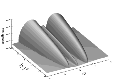
(a) $\quad\delta_{1}\delta_{2}=-3,0\leq|\gamma|^{2}\leq 5$

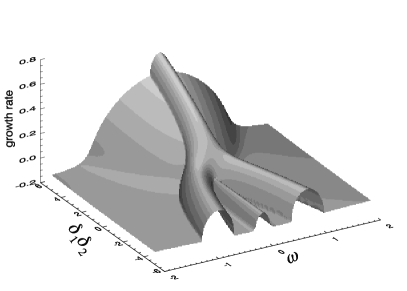
(b) $\quad|\gamma|^{2}=1,-5\leq\delta_{1}\delta_{2}\leq 5$

Figure 13: (a) Growth rates versus $|\gamma|^{2}$ and $\omega$. (b) Growth rates versus $\delta_{1}\delta_{2}$ and $\omega$ (b). Only the leading mode is shown. Details on the behavior at $|\gamma|^{2}=1$ and $\delta_{1}\delta_{2}=\pm 3$ can be extracted from Fig. 14. In both cases $\alpha^{r}_{1}=-0.1,\alpha^{r}_{3}=-0.2,\alpha^{i}_{1}=\alpha^{i}_{3}=0$, and $\epsilon=0.3$.

In the following, we always apply negative values for the unperturbed growth rates, i.e., we consider models with a magnetic Reynolds number below the dynamo threshold without the perturbation. The interaction parameters $|\gamma|^{2}$ and $\delta_{1}\delta_{2}$ are chosen such that characteristic and representative solutions are obtained with properties reminiscent of the simulations. Figure 13 shows the impact of the interaction parameters $|\gamma|^{2}$ and $\delta_{1}\delta_{2}$ for the case $\alpha_{1}^{r}=-0.1,\alpha_{3}^{r}=-0.2$ and $\alpha_{1}^{i}=\alpha_{3}^{i}=0$, with the perturbation amplitude fixed at $\epsilon=0.3$. For fixed $\delta_{1}\delta_{2}=-3$ the growth rates increase monotonically with $|\gamma|^{2}$ which parameterizes the interaction of $m=1$ and $m=-1$ modes (Fig. 13a). In contrast, the variation of $\delta_{1}\delta_{2}$, which parameterizes the interaction of $m=1$ and $m=3$ (respectively $m=-1$ and $m=-3$), may significantly change the structure of the growth rates (Fig. 13b).

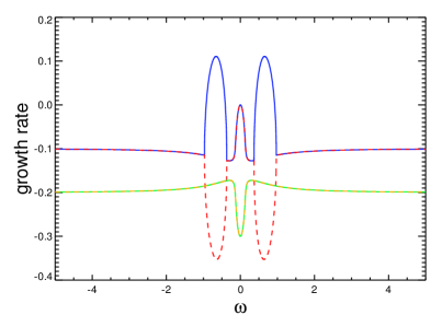
(a) Growth rates for $\delta_{1}\delta_{2}=-3$

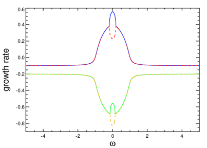
(b) Growth rates for $\delta_{1}\delta_{2}=+3$

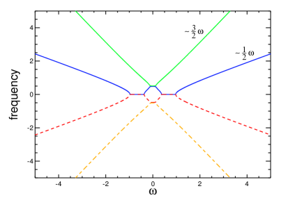
(c) Frequencies for $\delta_{1}\delta_{2}=-3$

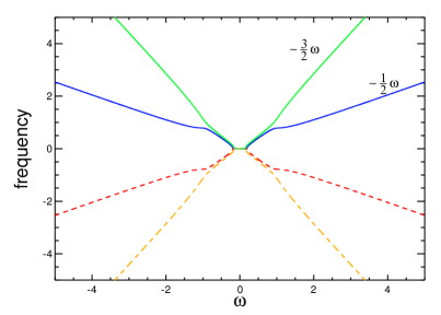
(d) Frequencies for $\delta_{1}\delta_{2}=+3$

Figure 14: Characteristic pattern of the growth rates (a,b) and frequencies (c,d) in dependence of $\omega$ for $\delta_{1}\delta_{2}=-3$ (a, c) and $\delta_{1}\delta_{2}=+3$ (b, d). For both cases $\alpha_{1}^{r}=-0.1,\alpha_{3}^{r}=-0.2,|\gamma|^{2}=1,\epsilon=0.3$. The blue and red curves denote the solutions belonging to $\widetilde{\sigma}_{1,2}$, and the green and orange curves denote the solutions belonging to $\widetilde{\sigma}_{3,4}$. Note that the frequency plots are not transformed into the original system.

Basically, we obtain two different types of solutions, which are shown in detail in Fig. 14. For a $\delta_{1}\delta_{2}<0$ the growth rates have three maxima, and we have two regimes with a parametric resonance symmetrically around the origin. The third maximum corresponds to a parametric amplification and is embedded between the parametric resonances. The pattern is rather similar to the behavior for small perturbation frequencies found in the simulations at ${\rm{Rm}}=120$ (see Figs. 7c and 7d). For a positive value of $\delta_{1}\delta_{2}$ we obtain one absolute maximum at $\omega=0$. However, in this case the single maximum emerges on top of a regime with amplification so that the overall pattern is different from the case shown in Figs. 7a and 7b.

The exemplary solutions show a combination of the phenomena that arose in the various limit cases discussed in the previous section. We find two resonance maxima symmetric with respect to the origin (for $\epsilon=0.3$ at $\omega_{\rm{max}}=\pm 0.65528$) resulting from the coupling of $m=1$ and $m=-1$ (see red and blue curves in Fig. 14a), but the resonance condition is no longer determined by a single and simple relation that involves the unperturbed frequencies $\alpha_{1}^{i}$ and/or $\alpha_{3}^{i}$. The location of the resonance maximum slightly depends on the amplitude of the perturbation. This is shown in Fig. 15, which presents the growth rates against $\omega$ and $\epsilon$ [Fig. 15(a)], the respective maximum against $\epsilon$ [Fig. 15(b)], and the increase of the maximum of the growth rate versus the perturbation amplitude $\epsilon$ [Fig. 15(c)].

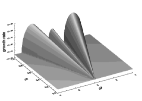
(a) Growth rate versus perturbation frequency $\omega$ and perturbation amplitude $\epsilon$

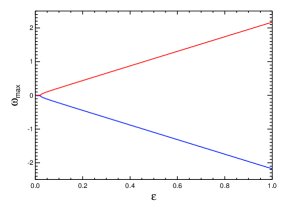
(b) Variation of the resonance frequency $\omega_{\rm{max}}$ with the perturbation amplitude

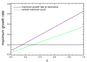
(c) Maximum of the growth rate versus perturbation amplitude

Figure 15: Characteristics of the eigenvalues for $\alpha_{1}^{r}=-0.1,\alpha_{3}^{r}=-0.2,\alpha_{1}^{i}=\alpha_{3}^{i}=0,|\gamma|^{2}=1$, and $\delta_{1}\delta_{2}=-3$.

Beside the linear dependence of the location of the regimes with parametric resonance on the perturbation frequency, a peculiar feature is the existence of the third maximum around the origin. This smaller third local maximum results from an indirect interaction between $m=\pm 1$ and $m=\pm 3$ without merging or splitting of the growth rates and without phase locking [see Fig. 14(c)]. A similar phenomenon has been found for small $\epsilon\mathrel{\mathchoice{\vbox{\offinterlineskip\halign{\hfil$\displaystyle#$\hfil\cr<\cr\sim\cr}}}{\vbox{\offinterlineskip\halign{\hfil$\textstyle#$\hfil\cr<\cr\sim\cr}}}{\vbox{\offinterlineskip\halign{\hfil$\scriptstyle#$\hfil\cr<\cr\sim\cr}}}{\vbox{\offinterlineskip\halign{\hfil$\scriptscriptstyle#$\hfil\cr<\cr\sim\cr}}}}0.1$ in the simulations at ${\rm{Rm}}=120$ (Fig. 7).

Regarding the frequencies, we abandon the presentation of the back-transformed frequencies in Fig. 14. We see a quite complex interaction of frequencies around the origin. Note in particular the merging and splitting of the frequencies that belong to the $m=-1$ and the $m=1$ branches [red and blue curve in Figs. 14c and d) which indicate the regions with phase locking. For large $\omega$ we obtain linear scalings $\propto\pm\nicefrac{{1}}{{2}}{\omega}$ and $\propto\pm\nicefrac{{3}}{{2}}{\omega}$ which after the back-transformation with $P(t)=e^{iD_{\omega}t}$ correspond to a behavior $\propto\pm\omega$ and $\propto\pm 2\omega$. Further complicated patterns are possible in particular when considering complex couplings and/or a nonvanishing frequency for the base modes ($\alpha_{1}^{i}$ and $\alpha_{3}^{i}$). In contrast to the previous cases, a nonvanishing imaginary part of an eigenvalue of the unperturbed state, like it occurs, for example in the case of a parity-breaking flow that yields azimuthally propagating eigenmodes, results in a system of equations that is no longer symmetric with respect to a sign change of the perturbation frequency $\omega$. This is shown, for example, in Fig. 16 with a clear asymmetric behavior with respect to $\omega$ when $\alpha_{1}^{i}\neq 0$.

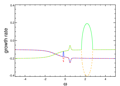
(a) Growth rates

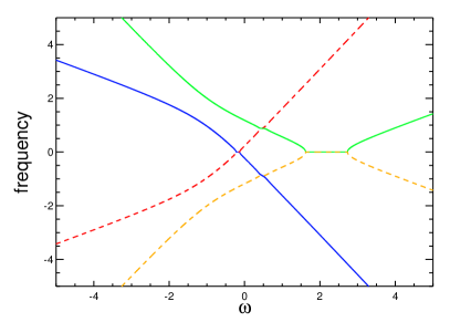
(b) Frequencies

Figure 16: Asymmetric behavior of growth rates (a) and frequencies (b) when the natural frequency of the system is $\neq 0$. $\alpha_{1}^{r}=-0.1,\alpha_{1}^{i}=1.0,\alpha_{3}^{r}=-0.2,\alpha_{3}^{i}=0,|\gamma|^{2}=1,\delta_{1}\delta_{2}=-3,\epsilon=0.3$. The blue and red curves denote the solutions belonging to $\widetilde{\sigma}_{1,2}$, and the green and orange curves denote the solutions belonging to $\widetilde{\sigma}_{3,4}$.

Nevertheless, as previously, we find that for sufficiently high frequencies the influence of the perturbation on the growth rate is negligible and the growth rates approach again their unperturbed values (but note the exchange of the $m=\pm 1$ and $m=\pm 3$ branches in Fig. 16). This behavior may allow an allocation of each curve to the original azimuthal modes and to determine which azimuthal modes couple or interact in order to form the coupled eigenfunction of the perturbed problem.

III.3.4 Cut off at $M=5$

Not surprisingly the behavior becomes more complex when increasing the truncation level to $M=5$. Here we abstain from specifying the characteristic equation which by virtue of its length and its complicated structure does not offer any additional insights. We limit ourselves to three examples that present typical solution patterns for growth rate and frequency (Fig. 17). The extension of the truncation level goes along with new parameters that describe the eigenvalues of the unperturbed new mode, denoted with $\alpha_{5}^{r}$ and $\alpha_{5}^{i}$, and the interaction of the new mode with itself and/or the $m=3$ mode, denoted by $\delta_{3}\delta_{4}$. Again we see a combination of resonances with phase locking and amplification, and we have a symmetric pattern with respect to the sign of the perturbation frequency as long as the imaginary parts of the involved dynamo modes and the coupling coefficients remain zero.

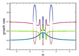
(a) $\alpha_{1}^{r}\!=\!-0.1,\alpha_{3}^{r}\!=\!-0.2,\alpha_{5}^{r}\!=\!-0.3,\alpha_{1,3,5}^{i}\!=\!0,\newline |\gamma|^{2}=1,\delta_{1}\delta_{2}=\delta_{3}\delta_{4}=-10$

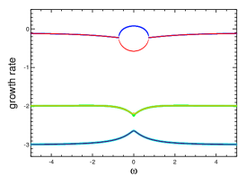
(b) $\alpha_{1}^{r}\!=\!-0.1,\alpha_{3}^{r}\!=\!-2.0,\alpha_{3}^{r}\!=\!-3.0,\alpha_{1,3,5}^{i}\!=\!0,\newline |\gamma|^{2}=1,\delta_{1}\delta_{2}=\delta_{3}\delta_{4}=-10$

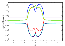
(c) $\alpha_{1}^{r}\!=\!-0.1,\alpha_{3}^{r}\!=\!-0.2,\alpha_{5}^{r}\!=\!-0.3,\alpha_{1,3,5}^{i}\!=\!0,\newline |\gamma|^{2}=5,\delta_{1}\delta_{2}=-3,\delta_{3}\delta_{4}=+3$

(d) $\alpha_{1}^{r}\!=\!-0.1,\alpha_{3}^{r}\!=\!-0.2,\alpha_{5}^{r}\!=\!-0.3,\alpha_{1,3,5}^{i}\!=\!0,\newline |\gamma|^{2}=1,\delta_{1}\delta_{2}=\delta_{3}\delta_{4}=-10$

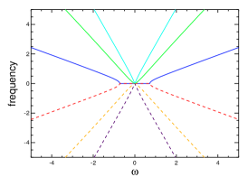
(e) $\alpha_{1}^{r}\!=\!-0.1,\alpha_{3}^{r}\!=\!-2.0,\alpha_{3}^{r}\!=\!-3.0,\alpha_{1,2,3}^{i}\!=\!0,\newline |\gamma|^{2}=1,\delta_{1}\delta_{2}=\delta_{3}\delta_{4}=-10$

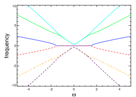
(f) $\alpha_{1}^{r}\!=\!-0.1,\alpha_{3}^{r}\!=\!-0.2,\alpha_{5}^{r}\!=\!-0.3,\alpha_{1,3,5}^{i}\!=\!0,\newline |\gamma|^{2}=5,\delta_{1}\delta_{2}=-3,\delta_{3}\delta_{4}=+3$

Figure 17: Growth rates (a,b) and frequencies (c,d) versus perturbation frequency for $\epsilon=0.3$ Note the large difference of the unperturbed growth rates on the case shown in (b) and (e). The red and blue (green and yellow, light-blue and violet) curves denote the solutions $\widetilde{\sigma}_{1,2}$ ($\widetilde{\sigma}_{3,4}$, $\widetilde{\sigma}_{5,6}$).

The behavior of the growth rates confirms the impression from the previous paragraph. A resonant behavior characteristic for a parametric instability with phase locking results only from the coupling of $m=1$ and $m=-1$ (blue and red curves in Fig. 17) whereas an interaction of $m=\pm 1$ with $m=\pm 3$ or $m=\pm 5$ happens only indirectly, producing a smoother parametric amplification patterns. Furthermore, we do not only see parabolic shapes around individual resonance maxima but also broader regimes composed of several local maxima [see, e.g., blue curves in Fig. 17(c)]. Particularly striking is the fact that the regimes with an enhancement of the growth rate are significantly broadened, allowing a transition from a stable solution to an unstable solution for a wide range of perturbation frequencies. The pattern becomes simpler when the original modes have larger differences in their unperturbed growth rates (Fig. 17b) so that the interaction of modes with different $|m|$ would require larger values for the corresponding interaction parameters.

III.4 The impact of the truncation level $M$

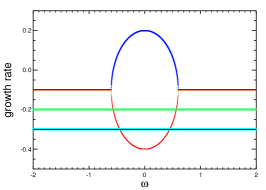
(a) $\delta_{1}\delta_{2}=\delta_{3}\delta_{4}=0$ corresponding to a truncation at $M=1$

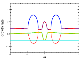
(b) $\delta_{1}\delta_{2}=-3,\delta_{3}\delta_{4}=0$ corresponding to a truncation at $M=3$

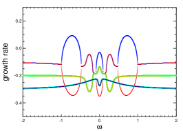
(c) $\delta_{1}\delta_{2}=-3,\delta_{3}\delta_{4}=-3$ corresponding to a truncation at $M=5$

Figure 18: Comparison of the solutions for the truncation level $M=1\cdots 5$ using different values for the interaction parameters $\delta_{1}\delta_{2}$ and $\delta_{3}\delta_{4}$. The plots correspond to solutions for increasing order of truncation. For all cases we use $\alpha_{1}^{r}=-0.1,\alpha_{3}^{r}=-0.2,\alpha_{5}^{r}=-0.3$, $\alpha_{1,3,5}^{i}=0$, $|\gamma|^{2}=1$, and $\epsilon=0.3$. The red and blue (green and yellow, light-blue and violet) curves denote the solutions $\widetilde{\sigma}_{1,2}$ ($\widetilde{\sigma}_{3,4}$, $\widetilde{\sigma}_{5,6}$).

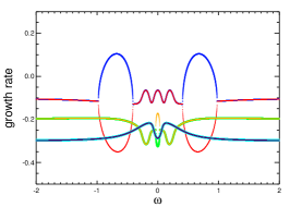
(a) $\delta_{3}\delta_{4}=1$

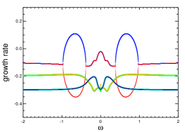
(b) $\delta_{3}\delta_{4}=0.3$

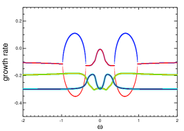
(c) $\delta_{3}\delta_{4}=0.1$

Figure 19: Comparison of the solutions for the truncation level $M=5$ and for decreasing values of $\delta_{3}\delta_{4}$. For all cases we use $\alpha_{1}^{r}=-0.1,\newline \alpha_{3}^{r}=-0.2,\alpha_{5}^{r}=-0.3$, $\alpha_{1,3,5}^{i}=0$, $|\gamma|^{2}=1,\delta_{1}\delta_{2}=-3,$, and $\epsilon=0.3$. The red and blue (green and yellow, light-blue and violet) curves denote the solutions $\widetilde{\sigma}_{1,2}$ ($\widetilde{\sigma}_{3,4}$, $\widetilde{\sigma}_{5,6}$).

The discussion of the impact of the truncation order is not straightforward, because when increasing the order from $M$ to $M+2$, new parameters get involved that parametrize the interaction of the new modes with themselves and with the adjacent mode with $m=M-2$. In fact, putting the new parameters to zero always leads to the solutions corresponding to the lower order truncation plus a solution of the type denoted in Eq. (66) for a single mode that emerges without interaction with the system. Figure 18 demonstrates the change in the solutions when increasing the truncation level. Note that for a truncation level $M=5$ the solutions for $\delta_{1}\delta_{2}=\delta_{3}\delta_{4}=0$ correspond to the solutions at order $M=1$ [Fig. 18(a)]. Likewise, for $\delta_{1}\delta_{2}\neq 0$ and $\delta_{3}\delta_{4}=0$ we recover the solutions at order $M=3$ [Fig. 18(b)].

Furthermore, the addition of new modes that come along with an increase of the truncation level results in a change of the structure of the solutions so that the behavior of the growth rates becomes more complex. The enlargement of the system by adding new modes always results in the emergence of new features in the pattern of the growth rates due to the interaction that become possible with the new modes. The structural changes become less important when the parameters that come along with increasing the truncation level decrease in amplitude. Figure 19 shows the results for a truncation at $M=5$ with a fixed parameter $\delta_{1}\delta_{2}=-3$ and for decreasing values of $\delta_{3}\delta_{4}$ (the parameter that describes the interaction between $m=\pm 3$ and $m=\pm 5$ modes). The resulting behavior of the growth rates corresponds to the smooth transition of the state shown in Fig. 18(c) to the state with $\delta_{3}\delta_{4}=0$ (corresponding to the truncation $M=3$) shown in Fig. 18(b). We conclude, that the analytical model only makes sense when for increasing truncation level the supervened parameters become negligible at a certain $M$ so that the consideration of further modes with large $M$ does not cause any further significant change in the structure of the solutions.

IV Discussion and Conclusions

We have examined dynamo action driven by a mean axisymmetric flow subject to spatio-temporal periodic perturbations. We have compared the outcome of a three-dimensional numerical dynamo model in cylindrical geometry with analytic results obtained from a simple low dimensional model for the magnetic field amplitude. Our computations show that a periodic excitation by means of a nonaxisymmetric flow perturbation can be beneficial for dynamo action when the perturbation frequency is in the right range. The essential properties shown by growth rates and frequencies of the eigenmode in the simulations can be qualitatively reproduced in the analytical model. This concerns in particular the occurrence of a localized strong increase of the growth rate and broader regimes with weaker enhancement when different azimuthal field modes are coupled. We also find less obvious details that occur in both approaches, like the symmetrical appearance of parametric resonances and the weak linear dependence of the location of the maximum on the amplitude of the perturbation. However, a quantitative agreement between the two models does not persist. This could not be expected because of the simplicity of the analytical model that does not take into account the particular geometry of the flow and is based on a decomposition of the magnetic field into azimuthal modes that are not exact eigenmodes of the (disturbed) system. In that sense our analytical approach is not equivalent to a perturbation method in a systematic mathematical meaning.

The parametric resonances found in our simulations are characterized by a strong gain in the growth rate in a narrow range of excitation frequencies, a nonoscillating amplitude of the field and the linking of the magnetic phase to the phase of the perturbation. The resonances have also been found in previous simulations with a different spatial structure of the periodic disturbance (see also our previous study Giesecke et al. (2012a)) as well as in our analytical model in which the shape of the disturbance is not specified at all. Hence we suppose that the shape of the perturbations is not important for the occurrence of the observed resonances.

Depending on the parameters in both approaches, simulations and analytical model, we obtain either a single peak around $\omega=0$ or two peaks symmetrical located around the origin. Broader regimes with an enhancement of the growth rates apparently emerge due to the coupling of eigenmodes with a different azimuthal wavenumber.

Our analytic model suggests that the parametric resonances in the perturbed system are based on the coupling of the azimuthal modes with the same modulus of the azimuthal wave number but with different sign ($m=1$ and $m=-1$ or $m=3$ and $m=-3$ in the example shown in Fig. 16). This corrects the speculations from our previous study where it was assumed that the parametric resonance in the perturbed dynamo is based on the interaction of $m=1$ and $m=3$ Giesecke et al. (2012a).

The analytical low-dimensional model is not intended to perfectly reproduce the simulations, which, indeed, is not even possible, because neither the basic flow field nor the pattern of the perturbation is considered in the low dimensional Ansatz. Instead it demonstrates how different eigenmodes of an unperturbed state become coupled by a perturbation and thus impact the dynamo ability of the system. In that sense the low dimensional model reflects some essential properties of our three-dimensional simulations and provides a plausible explanation for the complex behavior of the growth rates in different regimes with amplification of the field generation process like appear in our simulations at ${\rm{Rm}}=120$. Individual features, such as the single peak around $\omega=0$ for ${\rm{Rm}}=30$, the occurrence of the double maximum symmetrical about the origin with a smaller maximum in-between, or the existence of further broad secondary maxima without parametric resonance, are well reproduced. However, there is no real consistency between the analytic model and the simulations and a direct comparison or the reproduction of the particular pattern seen e.g. in Figs. 7c and  7d remains impossible.

The resonant behavior is similar to the behavior of periodically perturbed mechanical systems but the resonance condition only approximately fulfills the well-known relation $\omega_{\rm{res}}=2\omega_{0}$ (with $\omega_{0}$ the natural frequency of the unperturbed system) when a larger number of azimuthal field modes is involved. Furthermore, in accordance with the findings of Ref. Schmitt and Rüdiger (1992), the eigenvalues are no longer determined by a Mathieu-like equation even though the solutions show a similar behavior.

We find additional extended regimes with a significant enhancement of the growth rate but less pronounced than in the resonant case and without locking of the field to the phase of the perturbation. Our analytic model shows that the emergence of the amplification regimes requires the interaction of dynamo modes with distinct azimuthal wave numbers and a basic state which consists of dynamo modes with growth rates that are sufficiently close to each other. The vast regimes with parametric amplification have not been found in previous models, because either the higher magnetic field modes were not even considered (e.g., in the galactic dynamo models by Ref. Chiba and Tosa (1990)) or they decayed on a very fast time scale because the interaction triggered by the nonaxisymmetric perturbation has been too weak to become effective Giesecke et al. (2012a).

The very parametric resonance is limited to a narrow regime of rather small perturbation frequencies so that a realization in natural dynamos might be rather unlikely but cannot be ruled out. Nevertheless, the vast regimes with significant amplification caused by the interaction of modes with different azimuthal wave number in the analytical model and in the simulations may be still sufficient to turn a subcritical system into a dynamo with exponentially growing magnetic field even when the perturbation amplitude remains small. This nonresonant parametric amplification can also be of importance for long-term variations of magnetic activity as, for example, found in the solar dynamo models of Ref. Kitchatinov and Nepomnyashchikh (2015).

We have restricted our interest to linear models with a prescribed flow. However, it has been found that nonaxisymmetric perturbations also impact the nonlinear state of a dynamo Rohde et al. (1999) and may even change the fundamental character of the dynamo by triggering hemispheric asymmetries or cyclic changes of the large-scale magnetic field orientation known as flip-flop phenomenon or active longitudes Pipin and Kosovichev (2015). We further restricted our examinations to a perturbation pattern with azimuthal wave number $\widetilde{m}=2$ resulting, e.g., from tidal forces in a two-body system. A possible astrophysical application may be the impact on flow driving in planetary dynamos in particular when considering large Jupiter-like exo-planets that closely surround their host stars or resonance effects for stellar dynamo models Stefani et al. (2016). A possibility for a natural appearance of a perturbation pattern with higher azimuthal wave number, say, $\widetilde{m}=5$ and/or $\widetilde{m}=6$, are free inertial waves that can be excited via triadic resonances, e.g., in a precession driven flow Giesecke et al. (2015); Herault et al. (2015), which in turn may couple various magnetic field modes and thus improve the dynamo capability of the system.

It is tempting to make use of the beneficial impact of a space-time periodic regular perturbation on top of a given basic flow in order to excite dynamo action in experiments like the French von-Kármán-sodium (VKS) dynamo Monchaux et al. (2007) or the Madison dynamo Spence et al. (2006). Both experiments utilize a flow of liquid sodium driven by two opposing and counter-rotating impellers with the time-averaged flow similar to the flow applied in our study. So far the VKS dynamo exhibited magnetic field self-generation only in case of a flow driven by impellers made of a ferromagnetic alloy Miralles et al. (2013) whereas the Madison dynamo did not show dynamo action at all. For both experiments, a reduction of the critical magnetic Reynolds number by $30\%$, as found in our simulations, would be of great relevance. Interestingly, nonaxisymmetric vortex-like flow structures, which might represent the role of a suitable disturbance, were discovered for both configurations in water experiments ((de La Torre and Burguete, 2007; Ravelet et al., 2008; Cortet et al., 2009) in a cylinder) as well as in nonlinear three-dimensional simulations dedicated to the Madison dynamo Reuter et al. (2009). Kinematic dynamo simulations based on various manifestations of the flow field obtained from these nonlinear hydrodynamic simulations yield a beneficial impact of the nonaxisymmetric time-dependent flow perturbations, whereas neither the time-averaged flow nor time-snapshots of the velocity field were able to drive a dynamo Reuter et al. (2009). This effect was interpreted as dynamo action based on nonnormal growth Tilgner (2008). Nonnormal growth describes a perpetual increase of mode amplitudes by virtue of the appropriate mixing of nonorthogonal eigenstates even if the contributing eigenstates alone correspond to decaying solutions. However, in contrast to the dynamo models from Reuter et al. (2009) and Tilgner (2008) the boost of the growth rates observed in our study already occurs when applying stationary nonaxisymmetric perturbations and is not related to the time scale given by transient growth during the initial phase of the simulations which would depend on the initial conditions. Hence, we believe that the behavior found in our study is not based on nonnormal growth. In any case, our simulations show that, although perturbations are able to considerably boost the growth rates in a wide range of parameters (namely for a wide range of frequencies), a beneficial impact for the onset of dynamo action by reducing the critical magnetic Reynolds number can only be expected for stationary and/or slowly drifting nonaxisymmetric perturbations (much slower than the advective time scale based on the maximum axisymmetric azimuthal flow). Hence, the direct experimental realization of a beneficial impact provoked by the inherent nonaxisymmetric vortices is difficult because this would require a technical mechanism to control the azimuthal frequency of the observed nonaxisymmetric flow structures without significantly altering the basic flow field, which is hardly conceivable. More promising might be the flow driving mechanism at the Madison Plasma Dynamo Experiment (MPDX) Cooper et al. (2014) where a conducting unmagnetized plasma is exposed to a torque generated by external currents that interact with a multi-cusp magnetic field at the boundary. The resulting forcing drives a flow that is supposed to range deeply into the core plasma and may provide a possibility to impose appropriate nonaxisymmetric perturbations.