The Luminous Blue Variable RMC127 as seen with ALMA and ATCA

Abstract

We present ALMA and ATCA observations of the luminous blue variable RMC 127. The radio maps show for the first time the core of the nebula and evidence that the nebula is strongly asymmetric with a Z-pattern shape. Hints of this morphology are also visible in the archival HST $\rm H\alpha$ image, which overall resembles the radio emission. The emission mechanism in the outer nebula is optically thin free-free in the radio. At high frequencies, a component of point-source emission appears at the position of the star, up to the ALMA frequencies. The rising flux density distribution ($S_{\nu}\sim\nu^{0.78\pm 0.05}$) of this object suggests thermal emission from the ionized stellar wind and indicates a departure from spherical symmetry with $n_{e}(r)\propto r^{-2}$. We examine different scenarios to explain this excess of thermal emission from the wind and show that this can arise from a bipolar outflow, supporting the suggestion by other authors that the stellar wind of RMC 127 is aspherical. We fit the data with two collimated ionized wind models and we find that the mass-loss rate can be a factor of two or more smaller than in the spherical case. We also fit the photometry obtained by IR space telescopes and deduce that the mid- to far-IR emission must arise from extended, cool ($\sim 80\,\rm K$) dust within the outer ionized nebula. Finally we discuss two possible scenarios for the nebular morphology: the canonical single star expanding shell geometry, and a precessing jet model assuming presence of a companion star.

1. Introduction

It is widely accepted that the final destiny of a massive star is ruled by the mass-loss suffered during its post-Main Sequence (MS) evolution, and by how much mass remains at its death. For instance, the earliest O-type stars have to rapidly lose their hydrogen envelope (a few to a few tens of solar masses) in order to turn into Wolf-Rayet (WR) stars. The transition between the MS and the WR phase must be short, of the order of $10^{4}-10^{5}\,\rm yr$. Enhanced mass-loss is needed to reduce the envelope mass, through line-driven stellar winds or short-duration eruptions (e.g. Humphreys & Davidson, 1994; Smith & Owocki, 2006). The stars with the highest known mass-loss rates ($\dot{M}\gtrsim 10^{-5}\,\rm M_{\odot}\,yr^{-1}$) are the Luminous Blue Variable (LBV) stars, so called due to their location in the H-R diagram and because they show spectroscopic and photometric variability during a period of enhanced mass-loss caused by instabilities, as reviewed in Humphreys & Davidson (1994). These instabilities have yet to be conclusively explained, but several physical mechanisms have been proposed: vicinity to the (modified) Eddington limit due to an excess of radiation pressure; hydrodynamic (sub-photospheric) instabilities; rapid rotation and/or close-binary systems.

Smith & Tombleson (2015) noticed that the known Galactic and Magellanic LBVs tend to be isolated from massive star clusters. Hence they challenged the traditional single-star view of LBVs, proposing that the LBV phenomenon (strong instabilities and enhanced mass-loss) is instead due to interacting binaries, with a “mass donor” (e.g. WR star) and a “mass gainer” (LBV). The mass-transfer would “rejuvenate” the LBV star, whose evolution, as a consequence, would bifurcate from that of the other stars in the cluster where it formed. More recently, Humphreys et al. (2016) tested the same analysis for the LBVs in M31 and M33 and they also removed “seven stars with no clear relation to LBVs” from the sample of Smith & Tombleson (2015). Humphreys et al. (2016) then found that the LBVs distribute similarly to their O-type sisters or to the Red Supergiant (RSG) ones, depending on their initial mass and evolutionary state. Therefore, they revived the scenario for the evolution of a single massive star that approaches the Eddington limit.

The picture is still unclear and, due to the rarity of these objects, together with the rapid evolution of massive stars, we are still unable to put together all the pieces of the puzzle. On one hand it has been accepted that some LBVs and Ofpe (Bohannan & Walborn, 1989) super-giants are physically related, with the latter considered the quiescent state of a massive (O-type) LBV (e.g. Stahl, 1986). On the other hand, there is no evidence of their relationship with other massive stars, despite some suggestions: for instance, supergiant B[e] stars (Zickgraf et al., 1985, and following studies) and Of?p stars (the question mark indicates doubt that these stars are normal Of super-giants, Walborn, 1972, 1977). The B[e] supergiants are fast rotators and possess a dense and slow disk in their equatorial plane and a faster outflow along the polar axis. The Of?p stars have been found to be oblique magnetic rotators (Walborn et al., 2015, and ref. therein). Interestingly, the Galactic LBV AG Carinae (AG Car) has been found to be a fast rotator and its projected rotational velocity has been seen to change during LBV variability (Groh et al., 2006), but magnetic fields have not been detected in any known LBV.

The distinct morphologies observed in the nebulae around some candidate and confirmed LBVs, formed as a consequence of the intense mass-loss, suggest different shaping mechanisms (Nota et al., 1995). The morphologies of some nebulae are consistent with a symmetric mass-loss (e.g. Gal 79.29+0.46, S 61, Higgs et al., 1994; Weis, 2003; Umana et al., 2011b; Agliozzo et al., 2012, 2014, 2017a). However, the majority of the observed nebulae have a bipolar morphology (e.g. Weis, 2011) indicating aspherical mass-loss (e.g. Gal 026.47+0.02, Umana et al., 2012) or an external shaping mechanism (e.g. IRAS 18576+0341, HR Car, Umana et al., 2005; Buemi et al., 2010, 2017). Usually, bipolar or equatorial mass-losses have been proposed. Departure from spherical-symmetry has been directly observed in the winds of AG Car, HR Car and RMC 127 (e.g. Leitherer et al., 1994; Clampin et al., 1995; Schulte-Ladbeck et al., 1993), but whether aspherical mass-loss is an intrinsic property of LBVs has not been established (e.g. Davies et al., 2005). To explain LBVs with bi-polar or ring nebulae, enhancement of mass-loss in the equatorial plane of the star has often been invoked, the cause possibly being the fast rotation of the star, or the presence of a companion star, or a magnetic field (e.g. Gvaramadze et al., 2015, and ref. therein).

RMC 127 (HD 269858) is a well-known LBV located in the Large Magellanic Cloud. In the last decades it has been observed in both quiescent and active states, during which the stellar spectrum changed from Ofpe to A spectral types, through intermediate types B1–2, B7 and B9. At the beginning of the 2000s it began its decline towards the quiescent state (Walborn, 1977, 1982; Stahl et al., 1983; Wolf et al., 1988; Walborn et al., 2008). The first high-resolution image (Clampin et al., 1993) revealed the presence of a “diamond-shaped nebula” associated with the star. By means of spectro-polarimetric studies in the optical, Schulte-Ladbeck et al. (1993) found a high degree of polarization at the position of the star, similar to B[e] stars. They proposed two geometries for the stellar wind and the aligned outer optical nebula around RMC 127: a highly inclined bi-polar nebula or a disk or ring of material seen edge-on. This polarization was later confirmed by Davies et al. (2005). Smith et al. (1998) studied the kinematics of the nebula and they interpreted the data as two expanding shells (with the inner one $\lesssim$ 0.6 pc from the star). Later Weis (2003) obtained high resolution images in $\rm H\alpha$ with the Wide Field Planetary Camera 2 (WFPC2) on board the Hubble Space Telescope (HST). The authors described the nebula as comprising two Eastern and Western Rims and two Northern and Southern Caps. With a kinematic analysis of spectroscopic observations, they also reported that the Northern and Southern regions are blue- and red-shifted, respectively, with respect to the center of motion. Finally, RMC127 is a fast rotator, with a projected rotational velocity of $\sim 105\,\rm km\,s^{-1}$ (Agliozzo et al., 2017b).

In this paper we present a new dataset, acquired with ALMA and ATCA. We discuss the detection of a compact object associated with the central star from the centimeter (with ATCA) to the sub-millimeter (with ALMA). To understand the nature of this object, we complement the radio and sub-mm data with the IR photometry from space telescopes extracted from the public catalogs. Together with the central object, we also analyze the outer nebula that we detected with ATCA at 17 GHz. In this analysis we also include the maps at 5.5 and 9 GHz that were presented in Agliozzo et al. (2012, hereafter Paper I).

The paper is organized as follows: we present our dataset in Section 2. In Section 3 we analyze the radio and sub-mm emission, including the IR photometry from space telescopes. In Section 4 we discuss the central object emission and fit it with two Reynolds (1986) models for collimated ionized winds. In Section 5 we comment on different scenarios for the geometry of the outer nebula. Finally we summarize our results in Section 6.

2. Observations and data reduction

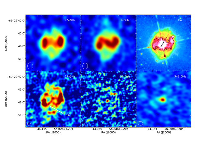
Figure 1.— From top-left to top-right: ATCA 5.5 and 9 GHz, and HST archival F656N $\rm H\alpha$ image. From bottom-left to bottom-right: ATCA 17 and 23 GHz, and ALMA 343.5 GHz. All images have the same field size. In each map, the synthesized beam is indicated with a white ellipse. At the lowest frequencies the emission from ionized gas in the nebula is detected and is co-spatial with the optical emission seen in $\rm H\alpha$. At the higher radio and sub-mm frequencies the central object is mostly the dominant component. In the optical image the black contour evidences hints of the bright Z-pattern shape visible, in particular, at 9 GHz. The white arrow and label (a) indicate the size of one diagonal arm (about 2.8 arcsec).

Table 1Summary of observations and images properties.

Date	Array	$\nu$	LAS	Synthesized Beam	PA	Peak	noise
		(GHz)	(arcsec)	FWHM (arcsec)	(deg)	(mJy beam-1)	(mJy beam-1)
2011-04-18/20	ATCA	5.5	22.0	1.53$\times$1.29	8.3	0.41	0.02
2011-04-18/20	ATCA	9	12.3	1.52$\times$1.17	3.4	0.40	0.03
2012-01-21/23	ATCA	17	6.5	0.82$\times$0.69	-8.0	0.17	0.02
2012-01-21/23	ATCA	23	4.1	0.62$\times$0.51	-8.0	0.16	0.03
2014-12-26	ALMA-LSB	337.5	9	1.26$\times$0.97	78.3	1.130	0.095
2014-12-26	ALMA	343.5	9	1.23$\times$0.95	78.4	1.140	0.072
2014-12-26	ALMA-USB	349.5	9	1.21$\times$0.93	78.6	1.18	0.11

2.1. ALMA observation and data reduction

RMC 127 ($\rm 05^{h}36^{m}43.688^{s}$ $\rm-69^{\circ}29^{\prime}47.52^{\prime\prime}$ ICRS) was observed as part of an ALMA Cycle-2 project studying three Magellanic LBVs (Project ID: 2013.1.00450.S), including LBV RMC 143 (Agliozzo et al. in prep) and candidate LBV S 61 (Agliozzo et al., 2017a, hereafter Paper II). The observations consisted of a single execution of 80 minutes total duration on 2014-12-26 with 40 12m antennas, with projected baselines from 10 to 245 m. The integration time per target was 16 minutes. A standard Band 7 continuum spectral setup was used, providing four 2 GHz-width spectral windows of 128 channels of XX and YY polarization correlations centered at approximately 336.5(LSB), 338.5(LSB), 348.5(USB) and 350.5(USB) GHz. Antenna focus was calibrated online in an immediately preceding execution, and antenna pointing was calibrated on each calibrator source during the execution (all using Band 7). Scans at the science target tuning on bright quasar calibrators QSO J0538-4405 and Pictor A (PKS J0519-4546; an ALMA secondary flux calibrator ‘grid’ source) were used for interferometric bandpass and absolute flux scale calibration. Astronomical calibration of complex gain variation was made using quasar QSO J0635-7516 interleaved with observations on the science targets approximately every six minutes.

As already mentioned in Paper II, atmospheric conditions were marginal for the combination of frequency and necessarily high airmass (transit elevation $43^{\circ}$ for RMC 127), requiring extra calibration steps in order to minimize image degradation due to phase smearing, to provide correct flux calibration and to maximize sensitivity by allowing inclusion of shadowed antennas. Details are presented in the Appendix, as they are expected to be of use for improving calibration for similar ALMA observations in marginal weather conditions at high airmass and/or with significant airmass difference between targets and gain calibrator (QSO J0635-7516), especially at bands 7 and above. This was performed in collaboration with staff at the Joint ALMA Observatory (JAO) who are working on these aspects of calibration.

In this work we used intensity images produced from naturally weighted visibilities in order to maximize sensitivity and image quality (minimize the impact of phase errors on the longer baselines). We imaged all spectral windows together ($343.5\,{\rm GHz}$ average; approximately $7.5\,{\rm GHz}$ usable bandwidth), obtaining an RMS noise of $0.072\,{\rm mJy}\,{\rm beam^{-1}}$ in the image. The proposed sensitivity of $40\,\mu{\rm Jy}\,{\rm beam^{-1}}$ could not be achieved as no further executions were possible during the appropriate array configuration in Cycles 2 and 3. Therefore, the nebula was not detected. The central object was instead detected at $15\sigma$.

We separately imaged the pairs of spectral windows in the two receiver sidebands ($337.5$ and $349.5\,{\rm GHz}$ centers; approximately $3.75\,{\rm GHz}$ bandwidth each), yielding RMS noise of $\sim\!0.10\,{\rm mJy}\,{\rm beam^{-1}}$ in the images. The two sideband images were used for an internal measure of the spectral index, and as a cross-check on the data quality. Fig. 1 illustrates the full bandwidth (7.5 GHz) map at 343.5 GHz. The synthesized beam is approximately $1.23^{\prime\prime}\times 0.95^{\prime\prime}$. Table 1 lists details of the observations and of the resulting images, including date of observations, interferometer, central frequency, largest angular scale (LAS), synthesized beam size (FWHM) and its position angle (PA), peak flux density on nebula and noise in the residual maps. Flux calibration uncertainty is estimated as 5% ($1\sigma$), although the peak flux may have a small additional systematic error to lower value due to residual phase smearing at a similar level. These uncertainties will be strongly correlated between the three images (average, LSB and USB) due to the small fractional frequency differences ($3.5$% between sideband centers) and minimal differences in atmospheric transmission, so the measurement of spectral index from only the ALMA data should be entirely noise-limited. Calibration and imaging of the ALMA data were performed using the Common Astronomy Software Applications (CASA) package, version 4.5 (McMullin et al., 2007).

2.2. ATCA data

The 17 and 23-GHz ATCA data of RMC 127 were obtained as part of observations of three magellanic LBV nebulae (Project ID: C1973), including RMC 143 and S 61. The observations were performed by using the array in the extended configuration (6-km) and the Compact Array Broadband Backend (CABB) receiver “15-mm Band” (16-25 GHz) during 2012 (see Table 1). We used observations of QSO J1924$-$2914, ICRF J193925.0$-$634245 and ICRF J052930.0$-$724528 for determining the bandpass, flux density and complex gain solutions, respectively. We also determined the polarization leakages and applied the solutions to the data in order to calibrate the cross-hands visibilities. Once corrected, the visibilities were inverted by Fourier transform. We imaged the I, V, Q and U Stokes parameters with a natural weighting for uv-data, for the best sensitivity. In the intensity map, we detected the nebula and the central object (see Fig. 1). We did not detect any polarization, as expected due to the low dynamic range. At 23 GHz there are positional errors in declination which are $\sim 0.4$ arcsec, almost half a synthesized beam. A source of error can be the fact that the phase calibrator was systematically at lower elevations than the science target. Given the poor weather and the proximity to the 22 GHz water line, systematic errors in the estimation of the atmospheric path length may contribute to this astrometric error. More information on these observations and data reduction can be found in the paper dedicated to S 61 (Paper II).

We also re-analyze the 5.5 and 9-GHz data from the ATCA observations performed in 2011 by using the CABB “4cm-Band” (4-10.8 GHz) receiver. These data were presented in Paper I. Here we reprocessed the data at 5.5 GHz by using a Briggs weighting scheme, with parameter robust=0, in order to match the angular resolution at 9-GHz. The ATCA maps are shown in Fig. 1 together with the ALMA one.

2.3. VISIR observations

We also observed RMC 127 at the Very Large Telescope (VLT) with the instrument VISIR, as part of a project including RMC 143 and S 61 (Project ID: 095.D-0433). An observing block in the narrow bandwidth filter PAH2$\_$2 (centered at 11.88 $\rm\mu$m) was successfully executed on 2015-11-01. The source was observed at an airmass of 1.6 and the seeing in the V-band was not better than 1 arcsec. The observing mode was set for regular imaging, with pixel scale of 0.045 arcsec. Four perpendicular nodding positions were used. RMC 127 was not detected, in part because the data were acquired for only $20\%$ of the desired total exposure time. According to the VISIR Exposure Time Calculator, for a point source of $40\,\rm mJy$ the signal-to-noise (S/N) would be $<3\sigma$ in each sub-images. Therefore the source could not be detected. We do not show the VISIR image because it is just noise, without detectable sources (the field of view is only $38\times 38$ arcsec²).

2.4. Hubble Space Telescope archival data

We retrieved from the STScI data archive the $\rm H\rm\alpha$ Hubble Space Telescope (HST) images of RMC 127 (Project ID: 6540), published by Weis (2003). The images were obtained with the Wide Field and Planetary Camera 2 (WFPC2) instrument using the $\rm H\rm\alpha$-equivalent filter F656N and reduced by the standard HST pipeline. We reprocessed the data as described in Paper I and II. We obtained a final image that matches with Weis (2003). We show it in the top line of Fig. 1.

3. Analysis and results

3.1. The ATCA and ALMA maps

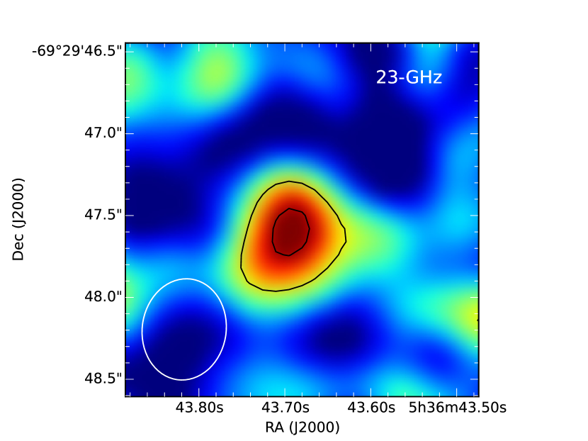
Figure 2.— Zoom-in of the ATCA 23 GHz map, centered on the central object. The white ellipse in the corner represents the synthesized beam. The 23 GHz contour levels corresponding to the 3 and 5$\sigma$ emission are plotted in black. The object appears slightly elongated, with a PA$\sim 110^{\circ}$, similar to the PA of the polarized emission detected by Schulte-Ladbeck et al. (1993). However, we cannot exclude noise contamination at the 3$\sigma$ level.

Table 2Central object peak flux density F_ν and nebula flux density S_ν at different frequencies.

$\nu$	Synthesized Beam	PA	Fν	Sν
(GHz)	(arcsec)	(deg)	(mJy beam-1)	(mJy)
5.5	1.53$\times$1.29	8.3	$<0.255$	3.1$\pm$0.2
9	1.52$\times$1.17	3.4	0.08$\pm$0.05	3.3$\pm$0.4
17	0.82$\times$0.69	-8.0	0.10$\pm$0.02	3.0$\pm$0.2
23	0.62$\times$0.51	-8.0	0.16$\pm$0.03	–
337.5	1.26$\times$0.97	78.3	1.130$\pm$0.095	–
349.5	1.21$\times$0.93	78.6	1.18$\pm$0.11	–

In Fig. 1 we show the interferometric radio and sub-mm maps of RMC 127 and we compare them with the archival HST $\rm H\alpha$ image, on the top-right. The resolution of the radio maps corresponds to the synthesized beam and is shown with white ellipses.

The radio maps reveal for the first time the inner part of the nebula. From low to high frequencies, different components dominate in the distribution of the emission. At low frequencies the nebula (very likely ionized by the central hot star) is the main source of radio emission, while at higher frequencies the central object dominates the emission. When the nebula is detected, the bipolar morphology is always evident. Previously, Weis (2003) recognized in the HST F656N $\rm H\alpha$ image an elongation culminating with the Northern and Southern caps. In the radio maps, in particular at 9 GHz, we notice an additional component at position angle (PA) $\sim 70^{\circ}$, a bar or a “diagonal arm”. This forms with the two Eastern and Western rims (“vertical arms”) a Z-pattern shape in the E-W direction. This is also visible in the HST F656N $\rm H\alpha$ image (see black contour in the top-right panel), despite the spikes and artifacts (due to the bright central star) that affect the appearance of the nebular morphology. The radio maps present indeed a new insight in the core of the nebula.

At 5.5 and 9 GHz the size of the nebula is approximately $7\times 6\,\rm arcsec^{2}$, or about $1.6\times 1.4\,\rm pc^{2}$ assuming a distance of $48.5\,\rm kpc$ for the LMC. The measured size is consistent with the estimate determined from the optical image (Weis, 2003). Since at 5.5 and 9 GHz the largest angular scale (LAS) is at least twice the size of the source (Table 1), we do not expect any significant loss of flux at these frequencies due to the sampling of the $uv$ plane.

At 17 GHz the source has the same extension and, roughly, the same morphology as at lower frequencies. However, the LAS is comparable to the source size; for this reason, even if the integrated flux density is preserved, artifacts can appear in the image. We spatially integrated the flux density at 17 GHz. The new measurement together with the 5.5 and 9 GHz values (reported in Paper I) are listed in Table 2. They are all consistent with thermal free-free emission (see Sec. 3.3). In Table 2 we also list the peak flux density at the central object position.

At 23 GHz the LAS is smaller than the source and, in fact, it is possible to detect only the compact central object and the edges of the nebula, while the extended flux is lost. At the ALMA frequency the LAS is comparable to or larger than the size of the nebula as seen at lower frequency. However, we only detect the compact central source. The nebula around it is barely discernible. This is probably caused by a low brightness of the source at the ALMA frequency compared with the RMS of the map. Assuming that the nebula emits through thermal optically thin free-free (Paper I), it is possible to estimate the total flux of the nebula at 343.5 GHz by extrapolating the measured flux density at low frequency with the typical power law ($S_{\nu}\sim\nu^{-0.1}$). The resulting flux density at 343.5 GHz is $\sim 2\,\rm mJy$. If we consider the number of ALMA beams in the nebula, this flux density corresponds to an average brightness of $0.14\,\rm mJy\,beam^{-1}$, which is only 2$\sigma$, therefore it was not detected. Note that with the completion of observations of the ALMA project (ID: 2013.1.00450S) it would have been possible to also detect the free-free emission in the nebula.

At 9-GHz the center of the nebula becomes as bright as the two rims. This is likely due to another emission component, which is partially resolved from the nebula at 17 GHz and also detected at 5$\sigma$ in the map at 23 GHz, where it appears as a compact source (Fig. 2). This object has an apparent elongation in nearly E-W direction at the 3$\sigma$ level. The position angle (PA) of this object is $\sim 110^{\circ}$, similar to the PA of the polarized emission detected by Schulte-Ladbeck et al. (1993). At the ALMA frequency the central object is the dominant emission component.

For the 23 GHz map, which is the highest-resolution map that we obtained, we used the task imfit of CASA to fit a 2-D Gaussian to the central object in the image-plane. The box region for the fit was selected around the $\sim 3\sigma$ contour level. The fit results in a Gaussian with FWHM=$0.71\pm 0.11$ arcsec along the major axis. The source is marginally resolved. The deconvolution from the synthesized beam gives a size of 0.43 arcsec in RA, equivalent to $\sim 3\times 10^{17}\,\rm cm$, or about 0.1 pc, at the distance of 48.5 kpc. However, at the 3$\sigma$ level the contours of this object could be still confused with the noise in the map. Hence, the size provided above must be considered an upper limit.

3.2. Spectral index of the central object

In Table 1 we report the peak flux density over the nebula. While at lower frequencies ($<$ 23 GHz) the peak brightness is in the right arm (Western rim) of the nebula, at 23 GHz and between 337.5 and 349.5 GHz the peak of the emission is at the position of the star. At these ALMA frequencies the peak flux density is almost three times higher than at 9 GHz (in the nebula), despite the ALMA synthesized beam being smaller.

The central object is not visible at 5.5 GHz. The reason can be confusion with the nebula emission, due to poor resolution at this frequency, combined with weaker emission. The latter possibility suggests a rising flux density distribution (e.g. $S_{\nu}\sim\nu^{\alpha}$), which is typical of stellar winds and self-absorbed emission. Note that the new map at 5.5 GHz has a synthesized beam almost identical to that at 9 GHz. We extract the peak flux density at 9 GHz ($0.36\pm 0.03\,\rm mJy$) at the position of the central object. Due to the low resolution this is contaminated by the emission from the “diagonal arm”. We then cut a slice along this arm, and fitted a Gaussian to the brightness profile in the slice along $\rm PA=70^{\circ}$. The distribution peak corresponds to a brightness of 0.28 mJy and $\sigma$= 0.05 mJy. We subtract this value from the peak flux density at the position of the central object and derive a brightness of $0.08\pm 0.05\,\rm mJy$ at 9 GHz. At higher frequencies we will refer to the peak flux densities in Table 2 extracted at the position of the central object. Their associated errors are the noise $\sigma$ as estimated in the residual maps (flux calibration errors are negligible).

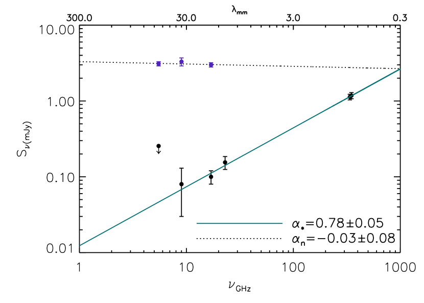
Figure 3.— Black points: peak flux densities at 5.5 (upper limit), 9, 17 and 23 GHz from the ATCA observations and at 337.5, 349.5 GHz from the ALMA observations, extracted at the position of the star. Solid line: weighted fit from 9 to 349.5 GHz. The positive slope suggests thermal emission from the ionized stellar wind. The spectral index $\alpha_{*}$ indicates departure from spherical symmetry with $n_{e}(r)\propto r^{-2}$. Purple points: spatially integrated flux densities of the nebula at 5.5, 9 and 17 GHz. Dashed line: fit from 5.5 to 17 GHz, characterized by an $\alpha_{n}$ typical of optically thin free-free emission in the ionized nebula.

We derive a weighted fit of the power-law ($S_{\nu}\sim\nu^{\alpha}$) between the centimeter and sub-millimeter flux densities of the central object (Fig. 3). This gives us a spectral index $\alpha$ of $0.78\pm 0.05$, which is higher than the canonical value for ionized winds with spherical symmetry and $n_{e}(r)\propto r^{-2}$ (Panagia & Felli, 1975; Wright & Barlow, 1975). Several mechanisms to explain the central object emission will be discussed in Section 4. A potential caveat with the flux density distribution may be the presence of systematic errors in each individual measurement (Table 2 and Fig. 3) due to the differing beam sizes and the nebular contributions to the extracted central object brightness in the maps. However, given the large frequency coverage (9 to 349.5 GHz) we are confident of the derived spectral index.

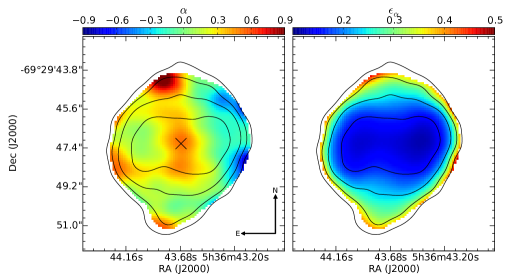
Figure 4.— Left: Spectral index map between 9 and 5.5 GHz. Contours show the isophotes of the 9 GHz image at the resolution of the 5.5 GHz data. The central component has a spectral index consistent with a thermal wind $\alpha\approx 0.6-0.7$. The emission of the two arms in the West and East directions have spectral index consistent with optically thin free-free emission $\alpha\approx 0$. Right: spectral index error map. The error associated with the spectral index map does non exceed 0.3 in most of the nebula. There is no evidence of non-thermal components.

3.3. Spectral index of the outer nebula

In Paper I we derived an average spectral index $\alpha\sim 0.1$ from the spatially-integrated flux densities at 5.5 and 9 GHz. With the new measurement at 17 GHz and the values from Paper I (see Table 2), the average spectral index is $-0.03\pm 0.08$ (Fig. 3), typical of optically thin free-free emission, with the flux density slightly decreasing at high frequencies and a theoretical power law $\propto\nu^{-0.1}$.

The images at radio wavelengths have angular resolution and sensitivity that allow us to study any deviation from the typical thermal free-free emission inside the nebula, by means of spectral index maps. The existence of non-thermal emission processes could indicate the presence of acceleration of particles up to the relativistic regime, due to shocks between the wind and the circumstellar environment, or due to the wind-wind interaction like in symbiotic systems, or other processes.

In colling wind binary (CWB) models for WR+O systems, the turnover frequency is usually lower than 5.5 GHz (e.g. Dougherty, 2010, and ref. therein). Therefore, in the observed range of frequencies, an hypothetical non-thermal component should be in the optically thin regime, with a negative spectral index. The maximum flux density is expected to be around 5.5 GHz or lower frequencies. Negative spectral indices should be evident in the spectral index map obtained by comparing the 5.5 and 9 GHz images. We prefer not to use the map at 17 GHz to derive spectral index maps, since, as reported in Section 3.1, artifacts can be present.

A spectral index map has been derived from the data at 5.5 and 9 GHz. For both bands, the LAS is much greater that the source and no flux is lost. The 9 GHz map has been convolved with a 2-dimensional Gaussian to match the beam at 5.5 GHz. After regridding the two maps in order to have the same pixel size, we computed the spectral index map and its associated error map (left and right panels of Fig. 4, respectively) in each common pixel $>3\sigma$. In the error map, the error in each pixel is dominated by the thermal noise (flux calibration errors are negligible). We also overlay the contours of the 9 GHz emission on top of the spectral index map. The mean spectral index over the nebula $\sim 0.0$ is still consistent with optically thin free-free emission from a nebular gas ionized by the central star. We exclude in our analysis the pixels at the borders, where the errors are high (up to 0.5). Around the central star $\alpha\approx 0.6$–$0.7$, which is consistent with an ionized wind. Along the diagonal arm, that is at $\rm PA=70^{\circ}$, $\alpha\approx-0.2$–$0.2$ which is consistent with a typical bremsstrahlung emission. Near the Northern and Southern caps we find similar values of $\alpha$, even if the associated error is much larger there. There is no evidence of a non-thermal component, at least at the resolution and sensitivity achieved by these observations.

3.4. The Spectral Energy Distribution from the near-IR to the radio

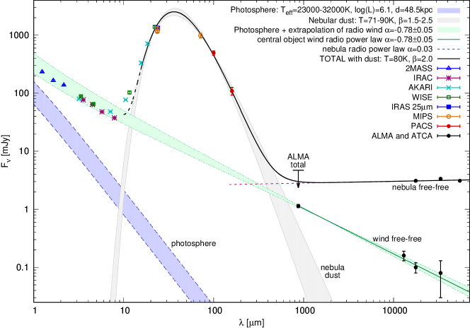
Figure 5.— SED of RMC 127 from near-IR to radio, including the photometry extracted from the IR catalogs of space telescopes and our ALMA and ATCA measurements. The arrow is the 3$\sigma$ upper limit to detect the whole nebula (dust + ionized gas) with ALMA. The gray band represents the fit gray-body functions obtained with a range of values for the parameter $\beta$ (between 1.5 and 2.5). The blue band represents several stellar photospheres derived assuming a stellar luminosity of $10^{6.1}\,\rm L\odot$ and an effective temperature range of $23000-32000$ K. The purple line is the fit of the radio nebula and the green line the fit of the central object, from the centimeter to the sub-millimeter. The green band was derived by taking into account the uncertainty of the radio spectral index. The wind free-free fit was extrapolated up to the near-IR wavelengths and summed with the photosphere emission. The black continuous line is the total emission from the mid-IR to the radio.

We queried the IR catalogs with the VizieR tool (Ochsenbein et al., 2000), and we extracted the flux densities of RMC 127 from 2MASS (Cutri et al., 2003), Spitzer/IRAC (Meixner et al., 2006), AKARI (Ishihara et al., 2010a, b), WISE (Cutri et al., 2012), IRAS (Beichman et al., 1988), Spitzer/MIPS (Whitney et al., 2008; van Aarle et al., 2011), and Herschel (Meixner et al., 2013). In Fig. 5 we plot the spectral energy distribution (SED) of RMC 127 from the near-IR to radio wavelengths. In addition to the two power-laws associated with the ionized nebula and with the stellar wind in the radio and sub-mm, it is also possible to recognize a component of cool dust commensurate with a gray-body. We also note that the photometry from about 1 to 8 $\rm{\mu m}$ traces neither a hot dust component close to the star nor cool dust in the outer nebula. The near-IR emission also shows an excess above the stellar photosphere (here we plot a range of reasonable effective temperatures for RMC 127 during its decline toward the quiescent state, e.g. Stahl et al., 1983; Walborn et al., 2008). Instead, the extrapolation of the stellar wind fit determined in the radio-mm range seems to account for the emission in the near-IR.

We fit the SED from the mid- to the far-IR with a single-temperature gray-body with power-law opacity index $\beta$. The slope in the Rayleigh-Jeans regime suggests high values for the parameter $\beta$, implying a grain size distribution dominated by small grains, similar to interstellar dust. The parameter $\beta$ is mostly constrained by the Herschel PACS photometry. We found a range of characteristic temperatures between $71$ to $90\,\rm K$ by varying $\beta$ between 1.5, 2 and 2.5 (extreme case). The gray-bodies that fit the data, taking into account their uncertainty, are represented in gray. The gray-body that best fits the data is plotted with a black solid line in Fig. 5, with $\beta=2.0$. At longer wavelength the black solid line is summed with the nebula free-free model, while at shorter wavelengths the total emission is not computed because of uncertainty of the wind spectral index and of the stellar effective temperature (green + blue bands). Furthermore, the mid-IR range around $10\,\rm\mu m$ is known to be complicated by solid state features that we cannot constrain.

The resulting characteristic temperature suggests that the mid- to far-IR emission arises from optically thin cool dust in the outer nebula (consistent with Bonanos et al., 2009). In the plot, the point indicated by the “ALMA total” label represents the 3$\sigma$ upper limit to detect the total emission over the nebula (the upper limit is derived from the rms noise in the maps integrated over the area corresponding the ionized nebula). The point-source detected with ALMA (black point) is clearly associated with the ionized gas in the stellar wind (Sec. 3.2).

4. The central object: discussion

The positive slope ($\alpha$=$0.78\pm 0.05$) of the radio flux density distribution (Sec. 3.2) indicates a thermal origin, so the emission must be associated with free-free encounters in the ionized stellar wind. This value deviates from the canonical case of a spherical wind with $n_{e}(r)\propto r^{-2}$ ($\alpha$=0.6, Panagia & Felli, 1975; Wright & Barlow, 1975). The spherical wind model requires an electron density distribution with a power-law steeper than -2 to reproduce such a spectral index.

None of the clumpy stellar wind models can reproduce the observed radio SED. In fact, optically thin clumps (micro-clumping case) do not alter the flux density distribution of the stellar wind at radio wavelengths (Nugis et al., 1998). Ignace (2016) recently showed that porous stellar winds (optically thick, macro-clumping) have a spectral index of $\nu^{0.6}$ if the porosity is in the form of shell-fragments (for any value of volume filling factor). If the clumps are spherical, and for extreme values of the filling factor, the flux density distribution can be shallower than $\nu^{0.6}$ and therefore produce an opposite effect to the RMC 127 case.

Daley-Yates et al. (2016) investigated the contribution due to the stellar wind acceleration region in the sub-mm, but they considered stars with relatively low mass-loss rates and with physical properties different from LBVs. The acceleration of the wind in RMC 127 very likely occurs much deeper in the wind, as indicated by the 2MASS points (see Fig. 5).

We recall that Schulte-Ladbeck et al. (1993) and Davies et al. (2005) found strong evidence of asphericity in the RMC 127 stellar wind, by means of optical spectro-polarimetry. Clampin et al. (1995) and Weis (2003) also suggested a deviation from spherical symmetry by morphological considerations of the outer nebula. This is also confirmed in the radio by our new interferometric maps. These results make unsuitable all the models based on spherical symmetry. As an alternative, we employ the Reynolds (1986) model of a collimated ionized stellar wind to explain the central object emission of RMC 127 in the radio and sub-mm. Ionized collimated stellar winds (jets) can have $-0.1<\alpha<2$ (Reynolds, 1986).

4.1. Collimated stellar wind models

Table 3Assumed and derived parameters for model 1 (isothermal, constant velocity, fully ionized conical outflow) and for model 2 (isothermal, constant velocity, well-collimated outflow with recombinations).

	Model 1	Model 2
$q_{v}$	0
$q_{T}$	0
$\vartheta_{0}$	0.5
$q_{x}$	0	-0.2
$\varepsilon$	1.34${}^{+0.15}_{-0.12}$	1.03${}^{+0.13}_{-0.10}$
$q_{n}$	-2.68${}^{+0.24}_{-0.29}$	-2.05${}^{+0.21}_{-0.26}$
$q_{\tau}$	-4.02${}^{+0.36}_{-0.44}$	-3.48${}^{+0.31}_{-0.38}$
$q_{\rm y}$	-0.52$\pm 0.05$	-0.60$\pm 0.06$
F	1.02$\pm 0.10$	1.18$\pm 0.12$

The Reynolds model can account for different configurations of the jet, described as power-law dependencies of the physical parameters along the jet (coordinate $r$ along the jet axis), such as jet width ($w\propto r^{\varepsilon}$), velocity ($v\propto r^{q_{v}}$), degree of ionization ($x\propto r^{q_{x}}$), temperature ($T\propto r^{q_{T}}$), and electron density $n_{\mathrm{e}}\propto r^{q_{n}}$ with $q_{n}=-q_{v}-2\varepsilon$. Assuming for the Gaunt factor $g_{\mathrm{ff}}\propto\nu^{-0.1}$, the absorption coefficient is $k_{\nu}\propto r^{q_{\tau}}$, where $q_{\tau}=\varepsilon+2q_{x}+2q_{n}-1.35q_{T}$.

Knowing the spectral index $\alpha$ of the wind, it is possible to determine how the jet width varies with distance (parameter $\varepsilon$), and therefore whether the jet is well-collimated or conical. The relationship between $\alpha$ and $\varepsilon$ is

$$\alpha=2+\frac{2.1}{q_{\tau}}(1+\varepsilon+q_{T})$$ (1)

In the case (Model 1) of an isothermal ($q_{T}=0$), fully ionized ($q_{x}=0$) and constant velocity outflow ($q_{v}=0$), with $\alpha$=$0.78\pm 0.05$ derived from the observations, $\varepsilon\approx 1.34$ and then, being $>1$, the jet opens toward the outside. Another interesting case (Model 2) to consider is that of an isothermal, constant velocity, exactly conical ($\varepsilon=1$) outflow with increasing recombinations ($q_{x}=-0.2$) as the plasma propagates outwards.

The mass-loss rate can be written in a general form that takes into account all these parameters (for details see Reynolds, 1986):

$$\dot{M}=5.27\times 10^{-9}\,v_{\infty\,\rm[km\,s^{-1}]}\,S_{\rm[mJy]}^{3/4}\,D_{\rm[kpc]}^{3/2}\,\nu_{\rm[GHz]}^{-3/4\alpha}\,T_{\rm[K]}^{-0.075}\times$$

$$\quad\quad\times\nu_{max\rm[GHz]}^{3/4\alpha-0.45}\,\frac{\mu}{x_{0}}\,\vartheta_{0}^{3/4}\,(\sin(\varphi))^{-1/4}\,F^{-3/4}\,[\rm M_{\odot}\,yr^{-1}],$$ (2)

where $F\equiv F(q_{\tau},\alpha)\equiv\frac{(2.1)^{2}}{q_{\tau}(\alpha-2)(\alpha+0.1)}$ .

In the equation we use the flux density $S$ at frequency $\nu=349.5\,\rm GHz$ and 48.5 kpc as distance $D$ of the object. We assumed $6420\pm 300\,\rm K$ for the gas temperature $T$ (Smith et al., 1998), whose influence on the mass-loss rate is very weak. For the terminal velocity of the wind we adopt $v_{\infty}=148\pm 14\,\rm km\,s^{-1}$ (Agliozzo et al., 2017b). The angle $\varphi=90^{\circ}-i$ formed between the jet axis and the line of sight is a free parameter, which only weakly affects the result due to the $-1/4$ power dependence. Here we assume $\varphi=75\,\rm\deg$ (thus $i=15\,\rm\deg$). Finally, we set to unity the ionized fraction $x_{0}$ at the base of the outflow and the mean atomic weight of the gas $\mu=1$ (assuming a gas of mostly hydrogen). Note that we do not know the jet opening angle $\vartheta_{0}$. An upper limit can be set equal to $0.5\,\rm rad$, a condition usually met in ionized jets (Mundt, 1985; Reynolds, 1986).

Another free parameter in Reynolds’ treatment is the maximum frequency $\nu_{max}$ in the SED, that we do not know. In fact, looking at Fig. 5, the extrapolation of the wind SED from the radio and sub-mm wavelengths seems to approach the emission of the star in the near-IR. However, it is important to note that the dependence of the mass-loss on $\nu_{max}$ is weak, since it goes as $\dot{M}\propto\nu_{max}^{0.135}$ in our case. A factor 100 in $\nu_{max}$ corresponds to a factor less than 2 in $\dot{M}$. It is further important to note that the Reynolds equations are based on the approximation of the Gaunt factor that is valid in the radio regime, and that at $\nu>10^{12}$ Hz it deviates more than 30% from the correct value. In addition, the cutoff of the free-free emission at high frequency, given by the factor $e^{-h\nu/KT}$, should be taken into account when extrapolating the Reynolds equations to the near-IR. The cutoff frequency corresponds to $10^{14}$Hz at $T\approx 6\,500$ K, i.e. a wavelength of a few microns. Furthermore, near the photosphere the wind is accelerated and it should be taken into account in the model. A reasonable value for $\nu_{max}$ seems to be $10^{13}$ Hz. For the two model scenarios we then have,

$$\dot{M}_{1,2}=C_{1,2}\,\left(\frac{D}{48.5\,\rm kpc}\right)^{\!1.5}\,\frac{v_{\infty}}{148\,\rm km\,s^{-1}}\,\left(\frac{\vartheta_{0}}{0.5}\right)^{\!0.75}\mu\,\times$$

$$\quad\quad\times\left(\frac{\nu_{max}}{10^{4}\,\rm GHz}\right)^{\!0.135}\,\sin(\varphi)^{-0.25}\,\times 10^{-6}\,[\rm M_{\odot}\,yr^{-1}]$$

with the only difference being the normalizations $C_{1}=9.4^{+2.6}_{-2.0}$ and $C_{2}=8.5^{+2.3}_{-1.8}$.

The mass-loss rate can be a factor of two or more smaller than in the spherical case ($2.1\pm 0.4\times 10^{-5}\,\rm M\odot\,yr^{-1}$), as deduced from the equation of Panagia & Felli (1975). As described in Reynolds (1986), the effect of collimated winds is to reproduce the radio flux density very efficiently, despite lower mass-loss rates than in the standard spherical case. This means that for unresolved radio stellar objects their mass-loss rates can be overestimated if the wind is not spherical.

Astrophysical objects that exhibit jets are usually associated with fast rotation and/or dense disks (e.g. Soker & Livio, 1994; Livio, 2000). We do not have evidence of a dense disk in our data (although Schulte-Ladbeck et al., 1993; Davies et al., 2005, suggested the presence of a disk at a few stellar radii), but we also do know that RMC 127 is a fast rotator (with a projected rotational velocity of $\sim 105\,\rm km\,s^{-1}$, Agliozzo et al., 2017b). A collimated outflow was discovered from the evolved B[e] star MWC137 (Mehner et al., 2016).

5. The outer nebula: discussion

The nebula associated with RMC 127 consists of dust and ionized gas, typical of LBVNe. In the radio the nebula emits mainly by free-free transitions (Sec. 3.3). The dust is very likely dominated by small grains, spread out over the ionized region, with an average temperature of $\rm T=80\pm 10\,K$ (Sec. 3.4). Using the flux densities extracted from the fits in Sec. 3.4 at the ALMA frequency 343.5 GHz (see Fig. 5), we derived a dust mass range of $M_{d}=2.2\times 10^{-3}$ to $2.2\times 10^{-2}\,\rm M\odot$, considering that $M_{d}=S_{\nu}\,D^{2}/(B_{\nu}(T)\,\kappa_{\nu})$, and assuming a $\kappa_{343\rm\,GHz}=1.7\rm\,cm^{2}\,g^{-1}$, as in Paper II for S 61. The range of dust masses in RMC 127’s nebula is consistent with typical values in LBVs, but suggests a lack of dust when compared to the RMC 127 Galactic twin, AG Car (e.g. Vamvatira-Nakou et al., 2015), although AG Car’s distance has been recently questioned (Smith & Stassun, 2017). A reduced dust mass of RMC 127 compared to AG Car could be due to the lower LMC metallicity.

The asymmetric expanding shell

According to the canonical view, RMC 127’s nebula is an expanding shell formed through past mass-loss events. The shell is not perfectly spherical and has an elongation in the N-S direction (Weis, 2003). The Northern and Southern Caps are also visible in the radio maps, especially at 5.5, 9 and 17 GHz (Fig. 1).

The cause of this asymmetry could have been a dense disk in the rotational plane of the star (Schulte-Ladbeck et al., 1993, nearly E-W direction). This disk channeled the wind along the polar axis and expanded more slowly than the ejecta at the higher stellar latitudes, causing a density anisotropy in the nebula. The radio emission co-spatial with the optical Eastern and Western Rims would be brighter because here the optical depth along the line of sight is larger. According to this scenario, closer to the star, there would be a similar system (consisting of a dense disk and a bipolar outflow) aligned with the outer nebula.

This scenario is akin to B[e] supergiants, which are fast rotators and have a dense disk in their equatorial plane and a fast outflow along the polar axis.

The precessing jet model

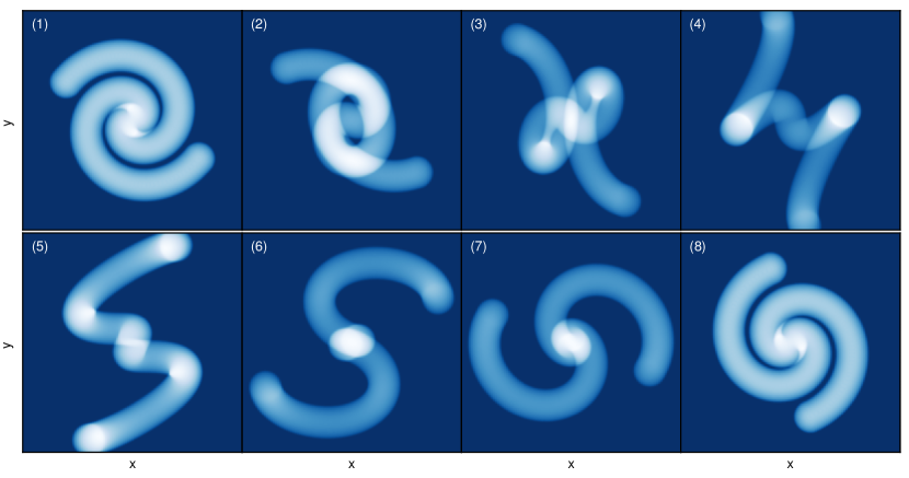
Figure 6.— Simulated 3-D conical helix (projected), as seen from eight different lines of sight (LOS). The viewing angles between the LOS and the three axes $(xyz)$ change continuously in panels (1) through (8). Each half-helix completed exactly one turn ($2\pi$). The helix “tube” diameter and height from origin along the system axis are 0.15 and 0.7, respectively, in relative units. The helix radius at any given height is $r(h)=h$. The simulation was created by using the new public code RHOCUBE (Nikutta & Agliozzo, 2016; Agliozzo et al., 2017a).

It is widely accepted that two thirds of massive stars are in binary or multiple systems. The interest in the effect of binarity on the evolution of massive stars has been increasing in recent years (e.g. De Marco & Izzard, 2017, and references therein). Recently a companion star of the Galactic LBV HR Car was directly detected (Boffin et al., 2016). On the basis of this discovery, Buemi et al. (2017) suggested a precessing jet model that can explain in part the complex HR Car nebular morphology. HR Car’s nebula is in fact characterized by an infrared inner shell and, in the perpendicular direction, a bipolar outflow of ionized gas, that resembles a helix. These features would be created under the influence of the binary or multiple system. Similarly to HR Car, RMC 127 has a collimated stellar wind. RMC 127 is also a fast rotator. RMC 127’s nebula could also have been formed through the bipolar outflow of a precessing star. To investigate this we used our new public code RHOCUBE (Nikutta & Agliozzo, 2016; Agliozzo et al., 2017a) to simulate a 3-D double conical helix nebula. Fig. 6 illustrates this simulated nebula as seen along eight different lines of sight. The three viewing angles w.r.t. the observer change continuously between panels (1) and (8) of the figure. We find a remarkable similarity of panel (2) in the figure with the 17-GHz morphology of RMC 127. The simulation was performed by assuming that the axial precession of the star has completed one period and that this corresponds to the kinematical age of the nebula. In this scenario, the polar axis is nearly in the E-W direction and is consistent with the first hypothesis by Schulte-Ladbeck et al. (1993), that the polarized emission could arise from a highly inclined bipolar outflow. The simulation in the figure does not have any quantitative relevance and is only shown to provide to the reader a schematic idea of the proposed scenario. Integral field unit spectroscopy in the future will allow to test this geometry. In the following, we proceed with a toy model to explore the possible implications and to eventually demonstrate that the hypothesis of the conical helix nebula is plausible.

The binary toy model

In the hypothesis that the jet precession toy model is valid, from kinematical considerations we can derive the precession period, but this requires an assumption on the velocity field in the outer nebula. Weis (2003) found an average projected velocity of $25\,\rm km\,s^{-1}$ along the two rims and of about $15\,\rm km\,s^{-1}$ along the two caps. For simplicity, we analyze the case of a jet expanding at constant velocity (set equal to the terminal velocity of the wind, $148\pm 14\,\rm km\,s^{-1}$, Agliozzo et al., 2017b). We consider then the size of the diagonal arm, $2.8\pm 0.4\,\rm arcsec$ (labeled “a” in Fig. 1), and derive a period of $4300\pm 700\,\rm yr$.

The axial precession motion would imply that the star must experience a tidal force, a torque of a companion star. Two other well-known LBVs in a binary and a multiple system are also bright in the X-rays. These are $\eta$ Car and HD5980 (Corcoran et al., 1995; Nazé et al., 2002). The class of LBVs is not overall intrinsically bright in the X-rays and the known X-ray emitters (in total four objects plus two candidates in the Galaxy, and one in the Small Magellanic Cloud) must be generally associated with an external factor, such as binarity (Nazé et al., 2012). Following the analysis of Nazé et al. (2012), a massive companion O-type star, that is a moderate X-ray emitter ($L_{X}\sim 10^{31}-10^{33}\,\rm erg\,s^{-1}$, Nazé et al., 2012), could be invisible at the X-ray wavelengths because of the strong absorption of the dense LBV wind, in the case of close orbits. However, wind-wind collisions should produce X-rays. Conversely, if the orbit is large, the intrinsic X-ray emission associated with the O-star would be visible, while the wind-wind interaction should not produce X-rays. A late-B companion of 3-6$\,\rm M\odot$ would not produce X-ray bright colliding wind emission, because its wind is negligible and would be invisible at X-ray wavelengths (Kashi, 2010). We searched the X-ray archives of $XMM-Newton$, $Chandra$ and $Swift$. One 28ks $XMM-Newton$ observation included RMC 127, however no X-ray photons are detected from its position. Assuming the distance of the LMC and the 1$\sigma$ sensitivity in the archive, the upper limit of X-ray luminosity in the 0.2-2.0 keV energy range is $L_{X}\lesssim 3\times 10^{34}\,\rm erg\,s^{-1}$ and in the 2.0-12.0 keV range is $L_{X}\lesssim 1\times 10^{35}\,\rm erg\,s^{-1}$. The X-ray observations did not reach the necessary sensitivity to detect sources as bright as the Magellanic system HD5980 (LBV+WR+O), which has X-ray luminosities of $L_{X}=1.7\times 10^{34}\,\rm erg\,s^{-1}$ in the range 0.3-10 keV and $L_{X}=9\times 10^{33}\,\rm erg\,s^{-1}$ in the range 0.2-2.4 keV (Nazé et al., 2002).

We analyze the case of an intermediate B-type companion for RMC 127, with mass $M_{2}=12\,\rm M\odot$, equivalent to a mass-ratio $q$ of 0.2, typical in observations of massive binary systems in our Galaxy (Kobulnicky et al., 2014). For the companion to exert a torque, RMC 127 must be not perfectly spherical and its equatorial plane must lie at an angle with the plane of the orbit. The angular velocity of the precession axis is $\Omega_{p}=\tau/I\Omega_{r}\sin(\theta)$, where $\theta$ is the angle formed by the rotational axis with the precession axis, $I$ the moment of inertia, $\Omega_{r}$ the angular velocity of the stellar axis. The magnitude of the torque is then $\tau=R_{*}\Delta F\sin(\theta)$, where $R_{*}$ is the stellar radius, $\Delta F$ is the gravitational force across the star’s width and is $\Delta F=2GM_{1}M_{2}\Delta r/a^{3}$, with $M_{1}$ and $M_{2}$ the masses of the two stars in the binary system and $G$ the gravitational constant. Therefore, the linear separation between the two stars $a$ is

$$a=\left(4\frac{GM_{1}M_{2}R_{*}^{2}\cos(\theta)}{I\Omega_{r}\Omega_{p}}\right)^{1/3}$$ (3)

To estimate the angular velocity $\Omega_{r}$ of RMC 127 we take the projected rotational velocity of $105\,\rm km\,s^{-1}$ (Agliozzo et al., 2017b) and the projection angle $i=15\,\rm\deg$ (consistent with our model in Section 4). If we assume as stellar radius $R_{*}$ = 50 R_☉ and mass $M_{1}$ = 60 M_☉ (Stahl et al., 1983), we obtain $\Omega_{r}\sim 1.2\times 10^{-5}\,\rm rad\,s^{-1}$, which corresponds to a period of $\sim 6$ terrestrial days. For the moment of inertia we approximate a solid sphere, given the small dependence of $a$ on $I$. From the precession period $T_{p}\simeq 4300\,\rm yr$ we derive $\Omega_{p}\sim 4.6\times 10^{-11}\,\rm rad\,s^{-1}$. Finally, based on the similarity between the simulation in Fig. 6 and the map at 17 GHz, we assume $\theta=45^{\circ}$.

In this examined case (companion of 12 M_☉) the inner separation $a$ between the two stars would be then $\sim 18\,\rm AU$ and the inner Lagrangian point L1 would be $\sim 12\,\rm AU$ ($\sim 51\,\rm R_{*}$), implying that the system is detached. However, when the primary star is at its maximum phase, the expanded pseudo-photosphere (stellar radius of $150\,\rm R_{\odot}$, Stahl et al., 1983) would fill the Roche lobe, implying mass transfer. The orbital period for this particular orbit would be about 9 yr. Boffin et al. (2016) derived for HR Car’s binary system a linear separation of 18 AU, an orbital period of 12 yr and a mass-ratio of 0.36. The presented exercise shows that the hypothesis of binarity for RMC 127 and axial precession is reasonable.

Noticeably, Lau et al. (2016) found an apparent precessing helical outflow associated with the Wolf Rayet star WR102c and attributed it to a previous phase of its evolution (namely, LBV). They also concluded that the helix is evidence of a binary interaction. They derived a precession period of 14000 yr.

The precessing jet model depends on the assumption of the binary nature of RMC 127, which has not yet been demonstrated. Given this, the single star expanding shell scenario appears the simplest description for the nebula. A long term, multi-wavelength observation campaign will be needed to conclusively distinguish these two scenarios and understand the nature of this complex object.

6. Summary

The ALMA and ATCA observations of RMC 127’s central object and outer nebula provide new insights of the nebula core of the classical LBV RMC 127. In the radio, at the lowest frequencies, the main component of emission is the ionized gas in the outer nebula, that resembles overall the $\rm H\alpha$ emission. The radio data permitted us to also analyze the inner part of the nebula, which in the optical is obscured by the bright central star. In addition to the previously known features in the nebula (Northern and Southern caps, Eastern and Western rims), we detected another emission component that gives to the nebula a strongly asymmetric aspect, a Z-pattern shape. We noticed a similar morphology in the HST $\rm H\alpha$ image.

The emission mechanism for the outer nebula in the radio is overall optically thin free-free with a global spectral index $\alpha$ of $-0.03\pm 0.08$. At higher frequencies a point-source component appears at the position of the star, bright up to the ALMA observing frequency of 349.5 GHz. This emission is due to thermal free-free emission in the ionized stellar wind. The stellar wind also seems to account for the excess at the near-IR wavelengths above the photosphere. The flux density distribution of the ionized wind (with spectral index $\alpha$=0.78$\pm$0.05) indicates a deviation from a spherical wind, supporting previous studies, and likely suggests the presence of a bi-polar outflow/jet. We fitted the data with two Reynolds (1986) models to determine the mass-loss rate in the jet, which can be at least a factor of two smaller than the case of spherical wind.

The fit of the mid- to far-IR flux densities derived from space telescope observations suggests that this emission arises from optically thin cool ($\sim 80\,\rm K$) dust spread out over the ionized region. The derived mass of the dust ($0.2-2.2\times 10^{-2}\,\rm M\odot$) is consistent with other Magellanic and Galactic LBVs.

We discussed two possible geometries to explain the outer nebula, including the canonical single star expanding shell model and a jet precession model assuming the presence of a companion star.

The asymmetry of the mass-loss geometry of RMC 127 may be strongly influenced by fast rotation and/or the presence of a companion star.

Appendix A Additional notes on the ALMA observation and data reduction

A standard Band 7 continuum spectral setup was used with the 64-input Baseline Correlator, giving four 2 GHz-width spectral windows (one per analogue baseband) of 128 channels ("TDM" mode, XX+YY polarization correlations) centered at approximately 336.5(LSB), 338.5(LSB), 348.5(USB) and 350.5(USB) GHz, with integration duration of 2.016 seconds. Companion channel-averaged correlator data with integration duration 1.008 second, and Water Vapor Radiometer (WVR) data with integration duration 1.152 second were also recorded. Time on source was approximately 16 minutes per target. Atmospheric conditions were marginal for the combination of frequency and necessarily high airmass (transit elevation $43^{\circ}$ for RMC 127), requiring extra calibration steps described below.

Of the 40 antennas, two had to be completely flagged (DA53, DV06), and another flagged completely in three of the four basebands (DA49 BB_2,3,4) due to intermittent coherence loss (a digitizer calibration problem affecting Walsh sequence phase switching). For one antenna (DV11) manual intervention was required in order to produce system temperature measurements (intermittent spurious values in the calibration device load temperature data). System temperatures were re-generated offline using the Cycle-3 TelCal software. Flags set by the online control software (XML flags) and by the correlator software (binary data flags) were applied as normal. In total 36 antennas were fully used in the reduction, with two more partially used due to issues in a subset of BBs/pols (DA49 BB_2,3,4; DA45 pol Y).

Online, antenna focus was calibrated in an immediately preceding execution, and antenna pointing was calibrated on each calibrator source during the execution (all using Band 7). Scans at the science target tuning on bright quasar calibrators QSO J0538-4405 and Pictor A (PKS J0519-4546; an ALMA secondary flux calibrator ‘grid’ source) were used for interferometric bandpass and absolute flux scale calibration. Astronomical calibration of complex gain variation was made using scans on quasar calibrator QSO J0635-7516 interleaved with scans on the science targets approximately every six minutes. The gain calibrator was a sub-optimal choice, as being six degrees further South than the targets it was at significantly higher airmass, with many antennas suffering some degree of shadowing. Data reduction proceeded as normal for ALMA data reduced in CASA, with the addition of the following modifications to deal with the combination of large airmass separation between science targets and gain calibrator, shadowing of antennas due to the compact configuration and low observing elevation, and generally marginal phase stability. We also evaluated the effect of calibrator source structure on the calibration.

A.0.1 Continuum WVR subtraction

Before running the wvrgcal program (Nikolic et al., 2012) which computes phase corrections from the WVR data, we pre-processed the raw WVR data to subtract a continuum contribution using a prototype algorithm implementation developed at JAO (W. Dent, priv. com.). This was developed to subtract the thermal continuum contribution produced by water droplets from the WVR channel temperatures, as wvrgcal assumes only water vapor emission. In this case it was primarily used to remove the thermal continuum due to shadowing (partially obstructed beam) from the WVR data, with the same reasoning. Reviewing the corrections applied to each antenna, compared with their predicted shadowing fraction for each scan, showed that this was successful, although in future the correction may improve by use of measured sky coupling efficiencies of each antenna+WVR combination (a topic of active investigation within the ALMA project).

A.0.2 Removal of WVR phase offsets between fields

Due to the large airmass separation between the science targets and the gain calibrator, combined with limitations in the calibration of the WVR data (a fixed sky coupling efficiency and channel frequencies are currently assumed) and limitations in the atmosphere model used to derive the phase corrections from the WVR data, we found phase offsets between fields in the phase correction table produced by wvrgcal, which differed between antennas and did not correspond to real phase offsets (confirmed by looking at self-calibration phase solutions for phase over all time on RMC 127– discrepant antennas corresponded to those with noted field offsets in the wvrgcal results). This effect is under investigation as part of ALMA’s continuing improvements to phase correction and antenna position determination. Without action, the image smearing due to these offsets made the WVR phase correction no significant improvement over not applying the correction. A simple solution of subtracting the field-averaged phase correction from the calibration table produced by wvrgcal was applied. This dramatically improved the image quality, resulting in over a 10% increase of the peak flux of RMC 127.

A.0.3 $T_{\rm sys}$ extrapolation between fields

The ALMA observation frequently measured the system temperature, $T_{\rm sys}$, at the location of the gain calibrator QSO J0635-7516. The standard ALMA data reduction applies this $T_{\rm sys}$ directly to the science fields, on the assumption that the difference is negligible due to proximity of the calibrator. This is a known limitation in ALMA’s amplitude calibration strategy – casa provides simple interpolation of $T_{\rm sys}$ in time (between scans) and frequency (within each $T_{\rm sys}$ spectral window), but not yet in airmass. For the dataset considered here, the $T_{\rm sys}$ error for the science targets by simply using that of the lower elevation gain calibrator was around 8–10%, with the error being largest for antennas which were more shadowed (larger blocking fraction) towards the gain calibrator. A simple $T_{\rm sys}$ extrapolation scheme was developed to correct this, using a simple model and the autocorrelation amplitude during each of the scans. This works for this dataset, as we used the TDM correlator mode, which produces linear autocorrelations (a quantization correction is applied in the correlator software, which cannot be applied in the higher resolution FDM mode). The channel-average autocorrelation data was used for this. The $T_{\rm sys}$ at the start and end of each scan was interpolated from the $T_{\rm sys}$ measurements on the gain calibrator using the following equation, taking an input $T_{\rm sys,1}$ and the autocorrelation values $V_{\rm 1}$, $V_{\rm 2}$ at the relevant times.

$$T_{\rm sys,2}=T_{\rm atm}\left(\frac{x}{1-x}\right);\quad x=\frac{T_{\rm sys,1}}{T_{\rm sys,1}+T_{\rm atm}}\frac{V_{\rm 2}}{V_{\rm 1}}$$ (A1)

A nominal atmosphere and blocking temperature $T_{\rm atm}=270\,{\rm K}$ was used, although the effect of varying this by plausible amounts was negligible for this case of $T_{\rm sys}\!\sim\!200\,{\rm K}$.

A.0.4 Source structure in gain calibrator QSO J0635-7516

We imaged the three calibrator sources in the execution as a cross-check of calibration and data quality. QSO J0538-4405 and Pictor A were point sources at the expected position. The gain calibrator, QSO J0635-7516, however showed significant source structure as shown in Fig. 7. This is a known mega-parsec scale jet discovered by Chandra (Schwartz et al., 2000) and previously imaged at centimeter and optical/near-IR wavelengths (e.g. Godfrey et al., 2012; Mehta et al., 2009). Since analysing our ALMA observation, maps from combination of calibrator scans in many ALMA observations have been presented by Meyer et al. (2017). To evaluate the effect of this structure on the phase calibration of the science targets, we used a clean component model of the source to both self-calibrate it and for correcting the phases of the other fields. The maximum in the residual self-calibration phases of QSO J0635-7516 was around $3^{\circ}$, and there was no significant effect on the image of RMC 127, so we concluded that the source structure of QSO J0635-7516 was irrelevant and it was a suitable calibrator choice in this regard (and it would be even less significant with smaller largest recoverable scale).

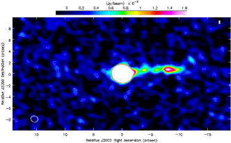
Figure 7.— ALMA Band 7 image ($343.5\,{\rm GHz}$, natural weighting, not primary beam corrected) of gain calibrator QSO J0635-7516, showing source structure in the jet to the West. The image is noise-limited with RMS noise of $0.15\,{\rm mJy}{\,\rm beam^{-1}}$, which is $1/3200$ of the central source. A single contour at $+2\sigma$ is overlaid. Synthesized beam size is $1.1^{\prime\prime}$.

References

- Agliozzo et al. (2012) Agliozzo, C., Umana, G., Trigilio, C., et al. 2012, MNRAS, (Paper I), 426, 181
- Agliozzo et al. (2014) Agliozzo, C., Noriega-Crespo, A., Umana, G., et al. 2014, MNRAS, 440, 1391
- Agliozzo et al. (2017a) Agliozzo, C., Nikutta, R., Pignata, G., et al. 2017a, MNRAS, (Paper II), 466, 213
- Agliozzo et al. (2017b) Agliozzo, C., et al. 2017b, conference proceeding “The mass-loss before the end: two luminous blue variables with a collimated stellar wind”, IAU-17-IAUS329, in press
- Beichman et al. (1988) Beichman, C. A., Neugebauer, G., Habing, H. J., Clegg, P. E., & Chester, T. J. 1988, Infrared astronomical satellite (IRAS) catalogs and atlases. Volume 1: Explanatory supplement, 1,
- Boffin et al. (2016) Boffin, H. M. J., Rivinius, T., Mérand, A., et al. 2016, A&A, 593, A90
- Bohannan & Walborn (1989) Bohannan, B., & Walborn, N. R. 1989, PASP, 101, 520
- Bonanos et al. (2009) Bonanos, A. Z., Massa, D. L., Sewilo, M., et al. 2009, AJ, 138, 1003
- Buemi et al. (2010) Buemi, C. S., Umana, G., Trigilio, C., Leto, P., & Hora, J. L. 2010, ApJ, 721, 1404
- Buemi et al. (2017) Buemi, C. S., Trigilio, C., Leto, P., et al. 2017, MNRAS, 465, 4147
- Clampin et al. (1993) Clampin, M., Nota, A., Golimowski, D. A., Leitherer, C., & Durrance, S. T. 1993, ApJ, 410, L35
- Clampin et al. (1995) Clampin, M., Schulte-Ladbeck, R. E., Nota, A., et al. 1995, AJ, 110, 251
- Corcoran et al. (1995) Corcoran, M. F., Rawley, G. L., Swank, J. H., & Petre, R. 1995, ApJ, 445, L121
- Cutri et al. (2003) Cutri, R. M., Skrutskie, M. F., van Dyk, S., et al. 2003, “The IRSA 2MASS All-Sky Point Source Catalog, NASA/IPAC Infrared Science Archive. ”
- Cutri et al. (2012) Cutri, R. M., Skrutskie, M. F., van Dyk, S., et al. 2012, VizieR Online Data Catalog, 2281,
- Daley-Yates et al. (2016) Daley-Yates, S., Stevens, I. R., & Crossland, T. D. 2016, MNRAS, 463, 2735
- Davies et al. (2005) Davies, B., Oudmaijer, R. D., & Vink, J. S. 2005, A&A, 439, 1107
- De Marco & Izzard (2017) De Marco, O., & Izzard, R. G. 2017, PASA, 34, e001
- Dougherty (2010) Dougherty, S. M. 2010, High Energy Phenomena in Massive Stars, 422, 166
- Godfrey et al. (2012) Godfrey L. E. H. et al. 2012, ApJ, 758L, 27
- Groh et al. (2006) Groh, J. H., Hillier, D. J., & Damineli, A. 2006, ApJ, 638, L33
- Gvaramadze et al. (2015) Gvaramadze, V. V., Kniazev, A. Y., Bestenlehner, J. M., et al. 2015, MNRAS, 454, 219
- Higgs et al. (1994) Higgs, L. A., Wendker, H. J., & Landecker, T. L. 1994, A&A, 291, 295
- Humphreys & Davidson (1994) Humphreys, R. M., & Davidson, K. 1994, PASP, 106, 1025
- Humphreys et al. (2014) Humphreys, R. M., Weis, K., Davidson, K., Bomans, D. J., & Burggraf, B. 2014, ApJ, 790, 48
- Humphreys et al. (2016) Humphreys, R. M., Weis, K., Davidson, K., & Gordon, M. S. 2016, ApJ, 825, 64
- Ignace (2016) Ignace, R. 2016, MNRAS, 457, 4123
- Ishihara et al. (2010a) Ishihara, D., Onaka, T., Kataza, H., et al. 2010, A&A, 514, A1
- Ishihara et al. (2010b) Ishihara, D., Onaka, T., Kataza, H., et al. 2010, VizieR Online Data Catalog, 2297,
- Kashi (2010) Kashi, A. 2010, MNRAS, 405, 1924
- Kobulnicky et al. (2014) Kobulnicky, H. A., Kiminki, D. C., Lundquist, M. J., et al. 2014, ApJS, 213, 34
- Lau et al. (2016) Lau, R. M., Hankins, M. J., Herter, T. L., et al. 2016, ApJ, 818, 117
- Leitherer et al. (1994) Leitherer, C., Allen, R., Altner, B., et al. 1994, ApJ, 428, 292
- Livio (2000) Livio, M. 2000, Asymmetrical Planetary Nebulae II: From Origins to Microstructures, 199, 243
- McMullin et al. (2007) McMullin, J. P., Waters, B., Schiebel, D., Young, W., & Golap, K. 2007, Astronomical Data Analysis Software and Systems XVI, 376, 127
- Meixner et al. (2006) Meixner, M., Gordon, K. D., Indebetouw, R., et al. 2006, AJ, 132, 2268
- Meixner et al. (2013) Meixner, M., Panuzzo, P., Roman-Duval, J., et al. 2013, AJ, 146, 62
- Mehner et al. (2016) Mehner, A., de Wit, W. J., Groh, J. H., et al. 2016, A&A, 585, A81
- Mehta et al. (2009) Mehta, K. T., Georganopoulos, M.; Perlman, E. S.; Padgett, C. A., Chartas, G. 2009, ApJ, 690, 1706
- Meyer et al. (2017) Meyer, E. T., Breiding, P., Georganopoulos, M., et al. 2017, ApJ, 835, L35
- Mundt (1985) Mundt, R. 1985, Protostars and Planets II, 414
- Nazé et al. (2002) Nazé, Y., Hartwell, J. M., Stevens, I. R., et al. 2002, ApJ, 580, 225
- Nazé et al. (2012) Nazé, Y., Rauw, G., & Hutsemékers, D. 2012, A&A, 538, A47
- Nikolic et al. (2012) Nikolic, B., Graves, S. F., Bolton, R. C., & Richer, J. S. 2012, Design and Implementation of the wvrgcal Program, ALMA Memo Series 593, The ALMA Project
- Nikutta & Agliozzo (2016) Nikutta, R., & Agliozzo, C. 2016, Astrophysics Source Code Library, ascl:1611.009
- Nota et al. (1995) Nota, A., Livio, M., Clampin, M., & Schulte-Ladbeck, R. 1995, ApJ, 448, 788
- Nugis et al. (1998) Nugis, T., Crowther, P. A., & Willis, A. J. 1998, A&A, 333, 956
- Ochsenbein et al. (2000) Ochsenbein, F., Bauer, P., & Marcout, J. 2000, A&AS, 143, 23
- Panagia & Felli (1975) Panagia, N., & Felli, M. 1975, A&A, 39, 1
- Reynolds (1986) Reynolds, S. P. 1986, ApJ, 304, 713
- Sault et al. (1995) Sault, R. J., Teuben, P. J., & Wright, M. C. H. 1995, Astronomical Data Analysis Software and Systems IV, 77, 433
- Schulte-Ladbeck et al. (1993) Schulte-Ladbeck, R. E., Leitherer, C., Clayton, G. C., et al. 1993, ApJ, 407, 723
- Schwartz et al. (2000) Schwartz, D. A. et al. 2000, ApJ, 540L, 69
- Smith et al. (1998) Smith, L. J., Nota, A., Pasquali, A., et al. 1998, ApJ, 503, 278
- Smith & Owocki (2006) Smith, N., & Owocki, S. P. 2006, ApJ, 645, L45
- Smith & Tombleson (2015) Smith, N., & Tombleson, R. 2015, MNRAS, 447, 598
- Smith & Stassun (2017) Smith, N., & Stassun, K. G. 2017, AJ, 153, 125
- Soker & Livio (1994) Soker, N., & Livio, M. 1994, ApJ, 421, 219
- Stahl et al. (1983) Stahl, O., Wolf, B., Klare, G., et al. 1983, A&A, 127, 49
- Stahl (1986) Stahl, O. 1986, A&A, 164, 321
- Umana et al. (2005) Umana, G., Buemi, C. S., Trigilio, C., & Leto, P. 2005, A&A, 437, L1
- Umana et al. (2011b) Umana, G., Buemi, C. S., Trigilio, C., et al. 2011, ApJ, 739, L11
- Umana et al. (2012) Umana, G., Ingallinera, A., Trigilio, C., et al. 2012, MNRAS, 427, 2975
- Vamvatira-Nakou et al. (2015) Vamvatira-Nakou, C., Hutsemékers, D., Royer, P., et al. 2015, A&A, 578, A108
- van Aarle et al. (2011) van Aarle, E., van Winckel, H., Lloyd Evans, T., et al. 2011, A&A, 530, A90
- Walborn (1972) Walborn, N. R. 1972, AJ, 77, 312
- Walborn (1977) Walborn, N. R. 1977, ApJ, 215, 53
- Walborn (1982) Walborn, N. R. 1982, ApJ, 256, 452
- Walborn et al. (2008) Walborn, N. R., Stahl, O., Gamen, R. C., et al. 2008, ApJ, 683, L33
- Walborn et al. (2015) Walborn, N. R., Morrell, N. I., Nazé, Y., et al. 2015, AJ, 150, 99
- Wang et al. (2004) Wang, W., Liu, X.-W., Zhang, Y., & Barlow, M. J. 2004, A&A, 427, 873
- Weis (2003) Weis, K. 2003, A&A, 408, 205
- Weis (2011) Weis, K. 2011, Bulletin de la Societe Royale des Sciences de Liege, 80, 440
- Whitney et al. (2008) Whitney, B. A., Sewilo, M., Indebetouw, R., et al. 2008, AJ, 136, 18
- Wright & Barlow (1975) Wright, A. E., & Barlow, M. J. 1975, MNRAS, 170, 41
- Wolf et al. (1988) Wolf, B., Stahl, O., Smolinski, J., & Casatella, A. 1988, A&AS, 74, 239
- Zickgraf et al. (1985) Zickgraf, F.-J., Wolf, B., Stahl, O., Leitherer, C., & Klare, G. 1985, A&A, 143, 421