On conditional cuts for Stochastic Dual Dynamic Programming

On conditional cuts for Stochastic Dual Dynamic Programming

Abstract

Multi stage stochastic programs arise in many applications from engineering whenever a set of inventories or stocks has to be valued. Such is the case in seasonal storage valuation of a set of cascaded reservoir chains in hydro management. A popular method is Stochastic Dual Dynamic Programming (SDDP), especially when the dimensionality of the problem is large and Dynamic programming is no longer an option. The usual assumption of SDDP is that uncertainty is stage-wise independent, which is highly restrictive from a practical viewpoint. When possible, the usual remedy is to increase the state-space to account for some degree of dependency. In applications this may not be possible or it may increase the state space by too much. In this paper we present an alternative based on keeping a functional dependency in the SDDP - cuts related to the conditional expectations in the dynamic programming equations. Our method is based on popular methodology in mathematical finance, where it has progressively replaced scenario trees due to superior numerical performance. We demonstrate the interest of combining this way of handling dependency in uncertainty and SDDP on a set of numerical examples. Our method is readily available in the open source software package StOpt.

1 Introduction

Dealing with uncertainty is vital in many real-life applications. An interesting way to formalize such a setting is a multistage stochastic program wherein one also accounts for the possibility of acting on past observed uncertainty. These models are quite popular in areas such energy [27, 50, 63, 57, 9], transportation [19, 34] and finance [54, 15, 14]. The usual underlying assumption is that uncertainty can somehow be presented or approximated using a scenario tree. The resulting mathematical programming problem is generally large-scale and non-trivial or impossible to solve using a monolithic method. The use of specialized algorithms that employ decomposition techniques (and very often sampling) appear crucial for an efficient numerical resolution. In this family two popular approaches are Nested Decomposition – ND – of [3] and Stochastic Dual Dynamic Programming – SDDP – of [51]. Mathematically speaking, both methods are close cousins, in that they approximate the cost-to-go functions (resulting from dynamic programming) using piecewise linear approximations, defined by cutting planes computed by solving linear programs in a so-called backward step.

The difference between the ND and SDDP algorithm resides in how uncertainty is handled when trying to establish an upper bound on the optimal value. The ND algorithm will use the entire scenario tree, whereas the SDDP algorithm will employ sampling procedures in order to achieve this. The ND algorithm therefore does not require any particular assumption on the scenario tree, but as a consequence is typically only applied to multistage stochastic problems of moderate size (with some hundred or a few thousand scenarios). In order to mitigate the effect that only “smaller” trees can be handled, methods for constructing representative but small scenario trees have therefore received significant attention. Let us mention the pioneering work [16] on two-stage programs and some subsequent extensions to the multistage case: e.g., [10, 52, 32, 53, 41]. Other ideas to reduce the computational burden rely on combining adaptive partitioning of scenarios with regularization techniques from convex optimization, e.g., [65, 66]. These ideas can also be extended to the multistage setting as done recently in [67].

It is therefore generally acknowledged that SDDP can handle larger scenario trees by combining decomposition and sampling, [51]. This method is highly popular as illustrated by the numerous applied papers, e.g., [10, 63, 34, 55, 27, 58]. The method however requires the assumption that the underlying stochastic process is stagewise independent (see also [8, 35, 12] for other methods employing sampling). Combined with a possibility to share cuts among different nodes of the scenario tree, the optimization strategies proposed in these references mitigate the curse of dimensionality further. However, the assumption that uncertainty is stagewise independent is quite a strong assumption when familiar with the actual observation of data. Whenever the underlying stochastic process is Markovian, it is generally suggested to increase the dimension of the state vector in order to revert back to a stagewise independence assumption (c.f., the discussion in [61]). As observed in [11] such an increase may be detrimental to computational efficiency especially if the increase in the dimension of the state vector is significant. The authors [11] suggest a way to partially mitigate this effect. In this paper we suggest another approach for efficiently estimating the conditional expectations appearing in the dynamic programming equations. The suggested method does not require increasing the size of the state vector whenever the underlying stochastic process is not stagewise independent. Our approach of estimating the conditional expectation is based on the observation that such expectations are orthogonal projections onto an appropriate functional space. The method suggested here is very popular in mathematical finance since the first work of Tsilikis and Van Roy [39] and the closely related Longstaff Schwarz method [44]. The latter has become the most used method to deal with optimal stopping problem, i.e., the optimization problem related to computing the optimal stopping time. The optimal stopping time is the best moment to exercise a given option. In the banking system, this method has become the reference method due to its easy implementation, its efficiency in moderate dimensions, and the easiness to calculate the sensibility of the optimal value (the “greeks”). In Energy market, quants use this method to valuate and hedge their portfolio (see [70] for an example of a gas storage hedging simulation).

In a recent paper, Bouchard and Warin [5] developed a variant of this method based on linear regression on adaptive meshes: they showed that this method was superior to the original Longstaff-Schwarz method based on global polynomial regression by avoiding oscillations of the regressor (the Runge effect). Indeed, the method was compared to different methods to price American options and to estimate the sensitivity of the options to the initial prices (the delta of the option) in dimension 1 to 6. In dimension 3 or above, the proposed regression method appeared to be clearly superior to optimal quantization [47, 46, 49, 48] and the Malliavin approach [21, 20]. Finally let us mention that the here suggested regression methods are also used to approximate conditional expectations in numerical schemes [4] used to solve Backward Stochastic Differential Equations (BSDE). The latter BSDEs provide a way to solve quasi-linear equations: the first papers [25, 42] have given birth to many follow up papers on the topic (see for example the references in the recent work of [26]). One can also use these building block to design schemes to solve full nonlinear equations [18].

To conclude the introduction, let us briefly mention that the mathematical properties of the SDDP algorithm have been extensively investigated. A first formal proof of almost-sure convergence of multistage sampling algorithms akin to SDDP is due to Chen and Powell [8]. This proof was extended by Linowsky and Philpott to cover the SDDP algorithm and other sampling-based methods in [43]. In fact both papers rely on a tacit assumption, formally worked out in [56]. Convergence in the general convex risk-neutral case is worked out in [24] and also studied in the risk-averse situation in [29]. Recent publications have addressed the issue of incorporating risk-averse measures into the SDDP algorithm: [30, 61, 55, 31, 63, 13, 36]. Polyhedral risk measures were studied in [17] and [30]. As mentioned in [63], theoretical foundations for a risk averse approach based on conditional risk mappings were developed in [59]. Extended polyhedral risk measures, also allowing for dynamic programming equations, can also be employed and where developed in [30]. It is shown is [61] how to incorporate convex combinations of the expectation and Average Value-at-Risk into the SDDP algorithm. Numerical experiments on this idea have been reported in many publications; see for instance [55] and [63].

This paper is organized as follows. Section 2 presents the general structure of multi-stage stochastic linear programs and show how the key difficulty resides in computing conditional expectations. We present the general idea of approximating conditional expectations in Section 3 and our algorithm in section 3.2. Finally Section 4 contains a series of numerical experiments showing numerical consistency of the suggested method. We also compare the method with other variants, wherein it appears that the suggested approach is preferable. The paper ends with concluding remarks and research perspectives.

2 Preliminaries on multistage stochastic linear programs and decomposition

Multistage stochastic programs explicitly model a series of decisions interspaced with the partial observation of uncertainty. If the given set of possible realizations of the underlying stochastic process is discrete, uncertainty can be represented by a scenario tree. Multistage stochastic linear programs (MSLPs) are a special case of this class wherein the underlying modelling structure is linear/affine. Hence, on a scenario tree the resulting model is a very large linear program. In this section we will provide an overview of two popular decomposition approaches for MSLPs, namely nested decomposition and stochastic dual dynamic programming. From an abstract viewpoint coming from non-linear non-smooth optimization, both methods are variants of Kelley’s cutting plane method [40].

Consider the following multistage stochastic linear program:

$$\min_{\overset{x_{1}\in X_{1}}{A_{1}x_{1}=b_{1}}}c_{1}^{\top}x_{1}+\mathbb{E}_{|\xi_{1}}\left[\min_{\overset{x_{2}\in X_{2}}{B_{2}x_{1}+A_{2}x_{2}=b_{2}}}c_{2}^{\top}x_{2}+\mathbb{E}_{|\xi_{[2]}}\left[\cdots+\mathbb{E}_{|\xi_{[T-1]}}[\min_{\overset{x_{T}\in X_{T}}{B_{T}x_{T-1}+A_{T}x_{T}=b_{T}}}c_{T}^{\top}x_{T}]\right]\right]\,,$$ (1)

where some of (or all) data $\xi=(c_{t},B_{t},A_{t},b_{t})$ can be subject to uncertainty for $t=2,\ldots,T$. The conditional expectation $\mathbb{E}_{|\xi_{[t]}}[\,\cdot\,]$ is taken with respect to the filtration generated by the history, up to time $t$, of the random vector $\xi_{t}\in\Xi_{t}\subseteq\mathbb{R}^{m_{t}}$, defining the stochastic process $\{\xi_{t}\}_{t=1}^{T}$. This history, up to time $t$, will be denoted with $\xi_{[t]}=(\xi_{1},\ldots,\xi_{t})$. Furthermore, $X_{t}\neq\emptyset$, $t=1,\ldots,T$, are polyhedral convex sets that do not depend on the random parameters, which we denote by $X_{t}:=\{x_{t}\in\mathbb{R}_{+}^{n_{t}}\mid D_{t}x_{t}=d_{t}\}$, for an appropriate matrix $D_{t}$ and vector $d_{t}$.

For numerical tractability, it is typically assumed that the number $N$ of realizations (scenarios) of the data process is finite, i.e., support sets $\Xi_{t}$ ($t=1,\ldots,T$) have finite cardinality. This is, for instance, the case in which (1) is a SAA approximation of a more general MSLP problem (having continuous probability distribution). For a discussion of the relation of such a problem with the underlying true problem relying on a continuous distribution we refer to [61]. In our numerical experiments we will also make this assumption.

Under these assumptions, the dynamic programming equations for problem (1) take the form

$$Q_{t}(x_{t-1},\xi_{[t-1]},\xi_{t}):=\left\{\begin{array}[]{llll}\displaystyle\min_{x_{t}\in\mathbb{R}^{n_{t}}}&c_{t}^{\top}x_{t}+\mathcal{Q}_{t+1}(x_{t})(\xi_{[t]})\\ \mbox{s.t.}&A_{t}x_{t}=b_{t}-B_{t}x_{t-1}\\ &x_{t}\in X_{t}\,,\end{array}\right.$$ (2)

where

$$\mathcal{Q}_{t+1}(x_{t})(\xi_{[t]}):=\mathbb{E}_{|\xi_{[t]}}[Q_{t+1}(x_{t},\xi_{[t]},\xi_{t+1})]\,,\quad\mbox{for }\;t=T-1,\ldots 1\,,$$ (3)

and $\mathcal{Q}_{T+1}(x)\equiv 0$ by definition. The first-stage problem becomes

$$\left\{\begin{array}[]{llll}\displaystyle\min_{x_{1}\in\mathbb{R}^{n_{1}}}&c_{1}^{\top}x_{1}+\mathcal{Q}_{2}(x_{1})(\xi_{[1]})\\ \mbox{s.t.}&A_{1}x_{1}=b_{1}\\ &x_{1}\in X_{1}\,.\end{array}\right.$$ (4)

An implementable policy for (1) is a collection of functions $\bar{x}_{t}=\bar{x}_{t}(\xi_{[t]})$, $t=1,\ldots,T$. Such a policy gives a decision rule at every stage $t$ of the problem based on a realization of the data process up to time $t$. A policy is feasible for problem (1) if it satisfies all the constraints for every stage $t$.

As in [61], we assume that the cost-to-go functions $\mathcal{Q}_{t}$ are finite valued, in particular we assume relatively complete recourse. Since the number of scenarios is finite, the cost-to-go functions are convex piecewise linear functions [62, Chap. 3].

We note that the stagewise independence assumption (e.g., as in [51]) simplifies (3) to $\mathcal{Q}_{t+1}(x_{t})(\xi_{[t]})=\mathcal{Q}_{t+1}(x_{t})=\mathbb{E}[Q_{t+1}(x_{t},\xi_{[t]},\xi_{t+1})]$ since the random vector $\xi_{t+1}$ is independent of its history $\xi_{[t]}=(\xi_{1},\ldots,\xi_{t})$. As pointed out in [61], in some cases stagewise dependence can be dealt with by adding state variables to the model. We will provide an alternative to that general methodology. We also care to note, and this will be a subsequent assumption, that whenever the data process is Markovian, than then $\mathcal{Q}_{t+1}(x_{t})(\xi_{[t]})$ depends on $\xi_{t}$ alone, i.e., $\mathcal{Q}_{t+1}(x_{t})(\xi_{[t]})\equiv\mathcal{Q}_{t+1}(x_{t})(\xi_{t})$.

First, let us briefly mention the main steps of ND and SDDP.

2.1 Decomposition

As already mentioned, two very important decomposition techniques for solving multistage stochastic linear programs are Nested Decomposition (see [60]), and the SDDP algorithm (see [51]). Both methods have two main steps:

• Forward step, that goes from stage $t=1$ up to $t=T$ solving subproblems to define feasible policies $\bar{x}_{t}(\xi_{[t]})$. In this step an (estimated) upper bound $\overline{z}$ for the optimal value is determined.

• Backward step, that comes from stage $t=T$ up to $t=1$ solving subproblems to compute linearizations that improve the cutting-plane approximations for the cost-to-go functions $\mathcal{Q}_{t}$. In this step a lower bound $\underline{z}$ is obtained.

Below we discuss these steps, starting with the backward one.

Backward step.

Let $\bar{x}_{t}=\bar{x}_{t}(\xi_{[t]})$ be a trial decision at stage $t=1,\ldots,T-1$, and $\check{\mathcal{Q}}_{t}$ be a current approximation of the cost-to-go function $\mathcal{Q}_{t}$, $t=2,\ldots,T$, given by the maximum of a collection of cutting planes. At stage $t=T$ the following problem is solved

$$\underline{Q}_{T}(\bar{x}_{T-1},\xi_{[T-1]},\xi_{T})=\left\{\begin{array}[]{llll}\displaystyle\min_{x_{T}\in\mathbb{R}^{n_{T}}}&c_{T}^{\top}x_{T}\\ \mbox{s.t.}&A_{T}x_{T}=b_{T}-B_{T}\bar{x}_{T-1}\\ &x_{T}\in X_{T}\end{array}\right.$$ (5)

for all $\xi_{T}=(c_{T},B_{T},A_{T},b_{T})\in\Xi_{T}$. Let $\bar{\pi}_{T}=\bar{\pi}_{T}(\xi_{T})$ be an optimal dual solution of problem (5). Then $\alpha_{T}(\xi_{T-1}):=\mathbb{E}_{|\xi_{T-1}}[b_{T}^{\top}\bar{\pi}_{T}]$ and $\beta_{T}(\xi_{T-1}):=-\mathbb{E}_{|\xi_{T-1}}[B_{T}^{\top}\bar{\pi}_{T}]\in\partial\mathcal{Q}_{T}(\bar{x}_{T-1})(\xi_{T-1})$ define the linearization

$$q_{T}(x_{T-1})(\xi_{T-1}) :=\beta_{T}^{\top}(\xi_{T-1})x_{T-1}+\alpha_{T}(\xi_{T-1})$$

$$=\quad\mathcal{Q}_{T}(\bar{x}_{T-1})(\xi_{T-1})+\langle\beta_{T}(\xi_{T-1}),x_{T-1}-\bar{x}_{T-1}\rangle\,,$$

satisfying

$$\mathcal{Q}_{T}(x_{T-1})\geq q_{T}(x_{T-1})\quad\forall\;x_{T-1}\,,$$

and $\mathcal{Q}_{T}(\bar{x}_{T-1})(\xi_{T-1})=q_{T}(\bar{x}_{T-1})(\xi_{T-1})$, i.e., $q_{T}$ is a supporting plane for $\mathcal{Q}_{T}$ (both functions of $\xi_{T-1}$). This linearization is added to the collection of supporting planes of $\mathcal{Q}_{T}$: $\check{\mathcal{Q}}_{T}$ is replaced by $\check{\mathcal{Q}}_{T}(x_{T-1})(\xi_{T-1}):=\max\{\check{\mathcal{Q}}_{T}(x_{T-1})(\xi_{T-1}),q_{T}(x_{T-1})(\xi_{T-1})\}$. In other words, the cutting-plane approximation $\check{\mathcal{Q}}_{T}$ is constructed from a collection $J_{T}$ of linearizations:

$$\check{\mathcal{Q}}_{T}(x_{T-1})(\xi_{T-1})=\max_{j\in J_{T}}\{\beta_{T}^{j\top}(\xi_{T-1})x_{T-1}+\alpha_{T}^{j}(\xi_{T-1})\}\,.$$

By starting with a model approximating the cost-to-go function from below (e.g. $\mathcal{Q}_{t}\equiv-\infty$ for all stages), the cutting-plane updating strategy will ensure that $\check{\mathcal{Q}}_{T}\leq\mathcal{Q}_{T}$. The updated model $\check{\mathcal{Q}}_{T}$ is then used at stage $T-1$, and the following problem needs to be solved for all $t=T-1,\ldots,2$:

$$\underline{Q}_{t}(\bar{x}_{t-1},\xi_{[t-1]},\xi_{t}) =\left\{\begin{array}[]{llll}\displaystyle\min_{x_{t}\in\mathbb{R}^{n_{t}}}&c_{t}^{\top}x_{t}+\check{\mathcal{Q}}_{t+1}(x_{t})(\xi_{t})\\ \mbox{s.t.}&A_{t}x_{t}=b_{t}-B_{t}\bar{x}_{t-1}\\ &x_{t}\in X_{t}\end{array}\right.$$ (9)

$$\equiv\left\{\begin{array}[]{llll}\displaystyle\min_{x_{t},r_{t+1}\in\mathbb{R}^{n_{t}}\times\mathbb{R}}&c_{t}^{\top}x_{t}+r_{t+1}\\ \mbox{s.t.}&A_{t}x_{t}=b_{t}-B_{t}\bar{x}_{t-1}\\ &\beta_{t+1}^{j\top}(\xi_{t})x_{t}+\alpha_{t+1}^{j}(\xi_{t})\leq r_{t+1},\quad j\in J_{t+1}\\ &x_{t}\in X_{t}\,.\end{array}\right.$$ (14)

Let $\bar{\pi}_{t}=\bar{\pi}_{t}(\xi_{t})$ and $\bar{\rho}_{t}^{j}=\bar{\rho}_{t}^{j}(\xi_{t})$ be optimal Lagrange multipliers associated with the constraints $A_{t}x_{t}=b_{t}-B_{t}\bar{x}_{t-1}$ and $\beta_{t+1}^{j\top}(\xi_{t-1})x_{t}+\alpha_{t+1}^{j}(\xi_{t-1})\leq r_{t+1}$, respectively. Then the linearization

$$q_{t}(x_{t-1})(\xi_{t-1}):=\beta_{t}^{\top}(\xi_{t-1})x_{t-1}+\alpha_{t}(\xi_{t-1})=\mathbb{E}_{|\xi_{t-1}}[\underline{Q}_{t}(\bar{x}_{t-1},\xi_{[t-1]},\xi_{t})]+\langle\beta_{t}(\xi_{t-1}),x_{t-1}-\bar{x}_{t-1}\rangle$$

of $\mathcal{Q}_{t}$ is constructed with

$$\alpha_{t}(\xi_{t-1}):=\mathbb{E}_{|\xi_{t-1}}[b_{t}^{\top}\bar{\pi}_{t}+\sum_{j\in J_{t+1}}\alpha_{t+1}^{j}(\xi_{t})\bar{\rho}_{t}^{j}]\quad\mbox{and}\quad\beta_{t}(\xi_{t-1}):=-\mathbb{E}_{|\xi_{t-1}}[B_{t}^{\top}\bar{\pi}_{t}]$$ (15)

and satisfies $\mathcal{Q}_{t}(x_{t-1})(\xi_{t-1})\geq q_{t}(x_{t-1})(\xi_{t-1})\;\;\forall\;x_{t-1}$.

Once the above linearization is computed, the cutting-plane model at stage $t$ is updated: $\check{\mathcal{Q}}_{t}(x_{t-1})(\xi_{t-1})=\max\{\check{\mathcal{Q}}_{t}(x_{t-1})(\xi_{t-1}),q_{t}(x_{t-1})(\xi_{t-1})\}$ . Since $\check{\mathcal{Q}}_{t+1}$ can be a rough approximation (at early iterations) of $\mathcal{Q}_{t+1}$, the linearization $q_{t}$ is not necessarily a supporting plane (but a cutting plane) for $\mathcal{Q}_{t+1}$: the inequality $q_{t}\leq\mathcal{Q}_{t}$ might be strict for all $x_{t-1}$ feasible (at the first iterations).

At the first stage, the following LP is solved

$$\underline{z} =\left\{\begin{array}[]{llll}\displaystyle\min_{x_{1}\in\mathbb{R}^{n_{1}}}&c_{1}^{\top}x_{1}+\check{\mathcal{Q}}_{2}(x_{1})(\xi_{1})\\ \mbox{s.t.}&A_{1}x_{1}=b_{1}\\ &x_{1}\in X_{1}\end{array}\right.$$ (19)

$$\equiv\left\{\begin{array}[]{llll}\displaystyle\min_{x_{1},r_{2}\in\mathbb{R}^{n_{1}}\times\mathbb{R}}&c_{1}^{\top}x_{1}+r_{2}\\ \mbox{s.t.}&A_{1}x_{1}=b_{1}\\ &\beta_{2}^{j\top}(\xi_{1})x_{1}+\alpha_{2}^{j}(\xi_{1})\leq r_{2},\quad j\in J_{2}\\ &x_{1}\in X_{1}\,.\end{array}\right.$$ (24)

The value $\underline{z}$ is a lower bound for the optimal value of (1). The computed cutting-plane models $\check{\mathcal{Q}}_{t}$, $t=2,\ldots,T$, and a solution $\bar{x}_{1}$ of problem (24) can be used for constructing an implementable policy as follows.

Forward step.

Given a scenario $\xi=(\xi_{1},\ldots,\xi_{T})\in\Xi_{1}\times\ldots\times\Xi_{T}$ (realization of the stochastic process), decisions $\bar{x}_{t}=\bar{x}_{t}(\xi_{[t]})$, $t=1,\ldots,T$, are computed recursively going forward with $\bar{x}_{1}$ being a solution of (24), and $\bar{x}_{t}$ being an optimal solution of

$$\left\{\begin{array}[]{llll}\displaystyle\min_{x_{t}\in\mathbb{R}^{n_{t}}}&c_{t}^{\top}x_{t}+\check{\mathcal{Q}}_{t+1}(x_{t})(\xi_{t})\\ \mbox{s.t.}&A_{t}x_{t}=b_{t}-B_{t}\bar{x}_{t-1}\\ &x_{t}\in X_{t}\end{array}\right.\equiv\left\{\begin{array}[]{llll}\displaystyle\min_{x_{t},r_{t+1}}&c_{t}^{\top}x_{t}+r_{t+1}\\ \mbox{s.t.}&A_{t}x_{t}=b_{t}-B_{t}\bar{x}_{t-1}\\ &\beta_{t+1}^{j\top}(\xi_{t})x_{t}+\alpha_{t+1}^{j}(\xi_{t})\leq r_{t+1},\quad j\in J_{t+1}\\ &x_{t}\in X_{t}\subseteq\mathbb{R}^{n_{t}},r_{t+1}\in\mathbb{R}\,.\end{array}\right.$$ (25)

for all $t=2,\ldots,T$, with $\check{\mathcal{Q}}_{T+1}\equiv 0$. Notice that $\bar{x}_{t}$ is a function of $\bar{x}_{t-1}$ and $\xi_{t}=(c_{t},A_{t},B_{t},b_{t})$, i.e., $\bar{x}(\xi_{[t]})$ is a feasible and implementable policy for problem (1) (up to stage $t$). As a result, the value

$$\overline{z}=\mathbb{E}\left[\sum_{t=1}^{T}c_{t}^{\top}\bar{x}_{t}(\xi_{[t]})\right]$$ (26)

is an upper bound for the optimal value of (1) as long as all the scenarios $\xi\in\Xi$ are considered for computing the policy. This is the case of nested decomposition. However, the forward step of the SDDP algorithm consists in taking a sample $\mathcal{J}$ with $M<N$ scenarios $\xi^{j}$ of the data process and computing $\bar{x}_{t}(\xi_{[t]}^{j})$ and the respective values $z(\xi^{j})=\sum_{t=1}^{T}c_{t}^{\top}\bar{x}_{t}(\xi_{[t]}^{j})$, $j=1,\ldots,M$. The sample average $\tilde{z}=\mathbb{E}_{|\mathcal{J}}[z(\xi)]$ and the sample variance $\tilde{\sigma}^{2}=\mathbb{E}_{|\mathcal{J}}[(z(\xi^{j})-\tilde{z})^{2}$ are easily computed. The sample average is an unbiased estimator of the expectation (26) (that is an upper bound for the optimal value of (1)). In the case of subsampling, $\tilde{z}+1.96\tilde{\sigma}/\sqrt{M}$ gives an upper bound for the optimal value of (1) with confidence of about $95\%$. As a result, a possible stopping test for the SDDP algorithm is $\tilde{z}+1.96\tilde{\sigma}/\sqrt{M}-\underline{z}\leq\epsilon$, for a given tolerance $\epsilon>0$. We refer to [61, Sec.3] for a discussion on this subject.

3 On Conditional cuts in SDDP

The assumption that the random data process is stagewise independent is useful in order to simplify the expressions given in section 2 such as (15). Essentially it deletes the additional dependency on the stochastic process of the cuts. This has a clear advantage in terms of storage, but the stagewise independence is also unrealistic in many situations. We will present here an alternative method for dealing with the conditional expectations that has the following advantages:

• There is no need to explicitly set up a scenario tree when initial data is available in the form of a set of scenarios $\left\{(\xi_{1}^{s},...,\xi_{T}^{s})\right\}_{s\in\mathcal{S}}$.

• There is no need to increase the dimension of the state-vector in order to account for stagewise dependency. Ways of handling dependency within SDDP are given in [28, 38], wherein the specific structure is exploited so as to efficiently “share” cuts. Similar ideas were successively exploited in [69] but not for SDDP. The methodology laid out in this work does not require making explicit such specific structure.

However our underlying assumption is that the random process is Markovian, i.e., the conditional distribution of $\xi_{t+1}$ knowing $\xi_{[t]}$ is the same as the conditional $\xi_{t+1}$ knowing $\xi_{t}$. We translate this here in the following form:

$$\xi_{t+1}=f_{t}(\xi_{t},\eta_{t}),$$ (27)

where the random data or innovation process $\eta_{t}\in\mathbb{R}^{p_{t}}$ is independent of $\xi_{[t]}$ and $f_{t}$ is a given map defined on $(\mathbb{R}^{m_{t}}\times\mathbb{R}^{p_{t}})$ with values in $\mathbb{R}^{m_{t+1}}$. This form (27) fits general time series models, such as AR, etc… (see e.g., [64]). Of course exploiting explicitly this structure to compute the conditional expectations, even if the distributions of $\eta_{t}$ are known is not easy.

A final approach to represent uncertainty, that we have not explicitly mentioned so far is the use of Markov Chains. We refer to [45, 55, 1] for some references incorporating SDDP and Markov Chains. Finite state Markov chains can of course explicitly be expanded into trees whenever necessary. Therefore in principle similar methodology can be employed. However much like our “criticism” of scenario trees, it is necessary to “create” a Markov chain if the initial data is available in the form of a set of scenarios. Since the Markov setting does not fit well the numerical experiments in the paper, we do not provide any comparison with it.

3.1 Dealing with conditional expectations - Linear Regression

One of the difficulties in solving problem (1) is closely tied in with evaluating conditional expectations. Indeed, e.g., equation (15) makes it apparent how this introduces an additional dependency with respect to the situation wherein only expectations are evaluated. The easiest way of computing conditional expectations is by setting up a tree or Markov chain to describe the evolution of $\xi_{t}$ and employ the transition probabilities to simply evaluate the conditional expectation. However, this approach, when only historical data is available, may lead to modelization errors by introducing an artificial representation of the underlying process in the form of a tree when only a set of samples of this process was available. Although the statistical quality of such a representation can be studied, we rather suggest to circumvent it altogether by directly employing a Monte Carlo approach both in the forward and backward steps.

We suppose that in the backward step the process is sampled through the Markovian dynamic of equation (27) once and for all with $S$ samples $\xi_{t}^{k}$ with $k=1,...,S$. This could be the result of having been able to fit a certain model to some original data, or having been given a model (e.g., electrical load could follow the dynamics of the model exhibited in [6]). Alternatively, these samples could simply be the historical data supposed to be Markovian. In the latter case, the data set could just be observed historical information (e.g., yearly electrical load over the past 30 years or so). At the end of this preprocessing step, a set of $S$ paths is available to work with.

It is well known that for any given $t$ the conditional expectation $\mathbb{E}_{|\xi_{t}}(.)$ is an orthogonal projection in the space of square integrable function so we will suppose in the sequel that all functions $g$ of $\xi=\left\{\xi\right\}_{t>0}$ of which we want estimate the conditional expectation satisfy $\mathbb{E}[g(\xi_{t})^{2}]<\infty$ for $t\leq T$ : such functions $g$ are said to be bounded in $L_{2}$. As a consequence, for any map $g:\Xi_{t+1}\rightarrow\mathbb{R}$, the conditional expectation satisfies $\mathbb{E}_{|\xi_{t}}(g(\xi_{t+1}))=F(\xi_{t})$ for a certain function $F:\Xi_{t}\rightarrow\mathbb{R}$. In order to keep the computational burden manageable as well as to limit storage requirements, we will assume that $F$ can be represented as a linear combination of a given set of base-functions. For instance, one could take Chebyshev or Legendre polynomials known to be an orthonormal basis for $L_{2}$ bounded functions as was originally proposed by [44].

Now for a fixed $t$ and given set $\psi_{t,1},\ldots,\psi_{t,P_{t}}$ of base functions the map $F$ can be approximated with the help of $S$ drawn samples by (linearly) regressing $\left\{g(\xi_{t+1}^{s})\right\}_{s=1}^{S}$ on $\left\{(\psi_{t,1}(\xi_{t}^{s}),...,\psi_{t,P_{t}}(\xi_{t}^{s}))\right\}_{s=1}^{S}$. This gives the following approximation:

$$\hat{\mathbb{E}}^{S}(g(\xi_{t+1})~{}|~{}\xi_{t})=\sum_{i=1}^{P_{t}}\alpha^{*}_{t,i}\psi_{t,i}(\xi_{t}),$$ (28)

where $\alpha^{*}_{t,1},...,\alpha^{*}_{t,P_{t}}$ is the optimal solution to the problem

$$\min_{\alpha_{1},...,\alpha_{P_{t}}}\sum_{s=1}^{S}\left(g(\xi_{t+1}^{s})-\sum_{i=1}^{P_{t}}\alpha_{i}\psi_{t,i}(\xi_{t}^{s})\right)^{2}.$$

Since the choice of an appropriate well performing basis (uniformly in $t$) and for a given set of instances of (1) may be tricky, we will consider instead the adaptive method developed in [5]. It relies on setting up a class of local base functions. In order to present the idea, let us denote with $\xi_{t,i}^{s}$ the $i$th coordinate of sample $s$ of $\xi_{t}\in\mathbb{R}^{m_{t}}$, where $i=1,...,m_{t}$. Now taking coordinate-wise extrema over the set of scenarios we define for each $i=1,...,m_{t}$, $\bar{\xi}_{t,i}=\max_{s=1,...,S}\xi_{t,i}^{s},$ $\underline{\xi}_{t,i}=\min_{s=1,...,S}\xi_{t,i}^{s}$. As shown in Figure 1, we now partition the set $\prod_{i=1}^{m_{t}}[\underline{\xi}_{t,i},\bar{\xi}_{t,i}]$ in a set of hypercubes $D_{t,\ell}$, $\ell=1,...,L_{t}$. For each given $\ell=1,...,L_{t}$, i.e., on each hypercube, we pick a family of mappings $\left\{\psi_{q}\right\}_{q\geq 0}$ having support on $D_{t,\ell}$. Typically the family $\left\{\psi_{q}\right\}_{q\geq 0}$ will be that of all monomials in $\mathbb{R}^{m_{t}}$, implying that $m_{t}+1$ coefficients need to be stored for each element $\ell=1,...,L_{t}$ of the partition. We emphasize that the approximation is nonconforming in the sense that we do not assure the continuity of the approximation. However, it has the advantage to be able to fit any, even discontinuous, function. The total number of degrees of freedom is equal to $(1+m_{t})L_{t}$ which quality-wise should be related to the sample size $S$. Hence, in order to avoid oscillations, the partition is set up so that each element roughly contains the same number of samples. Using this approximation, the normal equation is always well conditioned leading to the possibility to use the Choleski method, which, as shown in [5], is most efficient for solving the regression problem. We even note that the problem can be decomposed in $L_{t}$ regressions with $m_{t}\times m_{t}$ regression matrices. Using a partial sort algorithm in each direction it is then possible to get roughly the same number of samples in each cell as explained in [5]. The use of this partitioning procedure is illustrated on Figure 1.

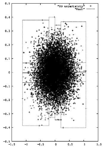
Figure 1: Example of the support of the local basis functions in dimension 2. Here $4$ intervals are chosen for each direction giving a total of $L=16$ hypercubes.

As explained in the introduction, the numerical results presented in [5] demonstrate the superiority of this local method with respect to various competing ways of estimating conditional expectations such as quantization or Malliavin regression. We note that a constant per mesh approximation can be used instead of a linear one, giving a far less efficient method if the functions to approximate are regular or piecewise regular.

3.2 The SDDP algorithm with conditional cuts and local base functions

In this section we provide the description of our variant of the SDDP algorithm relying on conditional cuts and using local base functions. A variant using only global base functions is readily extracted. In the algorithm below, we add the index $s$ to emphasize the dependency of the data on the scenario. Let us also note that for a given current trial decision $\bar{x}_{t}=\bar{x}_{t}(\xi_{[t]})$ at stage $t$, that this can be associated with a given mesh $D_{t,h(t)}$, for $h(t)\in\{1,...,L_{t}\}$. The value $h(t)$ is such that $\xi_{t}\in D_{t,h(t)}$. We will emphasize this by speaking of the trial decision $(\bar{x}_{t},h(t))$.

Backward step.

Let $(\bar{x}_{t},h(t))$ be a trial decision at stage $t=1,\ldots,T-1$ and $\check{\mathcal{Q}}_{t}$ be a current approximation of the cost-to-go function $\mathcal{Q}_{t}$, $t=2,\ldots,T$, given by the maximum of a collection of (functional) cutting planes. At stage $t=T$ the following problem is solved for all $s$ such that $\xi_{T-1}^{(s)}\in D_{T-1,h(T-1)}$

$$\underline{Q}_{T}(\bar{x}_{T-1},\xi_{T}^{(s)})=\left\{\begin{array}[]{llll}\displaystyle\min_{x_{T}\in\mathbb{R}^{n_{T}}}&(c_{T}^{(s)})^{\top}x_{T}\\ \mbox{s.t.}&A_{T}^{(s)}x_{T}=b_{T}^{(s)}-B_{T}^{(s)}\bar{x}_{T-1}\\ &x_{T}\in X_{T}\end{array}\right.$$ (29)

Let $\bar{\pi}_{T}^{(s)}$ be an optimal dual solution of problem (29). Now let $\alpha_{T}(y)$, $\beta_{T}(y)$ be the numerically approximated conditional expectations of $b_{T}^{\top}\bar{\pi}_{T}$ and $B_{T}^{\top}\bar{\pi}_{T}$ respectively while employing the estimates of (28). We will denote this as $\alpha_{T}(y):=\hat{\mathbb{E}}^{S}[b_{T}^{\top}\bar{\pi}_{T}|\xi_{T-1}=y]$ and $\beta_{T}(y):=-\hat{\mathbb{E}}^{S}[B_{T}^{\top}\bar{\pi}_{T}|\xi_{T-1}=y]$.

Now define the linearization

$$q_{T}(x_{T-1})(\xi_{T-1}) :=\beta_{T}^{\top}(\xi_{T-1})x_{T-1}+\alpha_{T}(\xi_{T-1})$$

$$=\hat{\mathbb{E}}^{S}\left[\underline{Q}_{T}(\bar{x}_{T-1},\xi_{T})|\xi_{T-1}\right]+\langle\beta_{T}(\xi_{T-1}),x_{T-1}-\bar{x}_{T-1}\rangle.$$

This linearization is used to update the current cutting plane model as follows:

$$\check{\mathcal{Q}}_{T}(x_{T-1})(\xi_{T-1}):=\max\{\check{\mathcal{Q}}_{T}(x_{T-1})(\xi_{T-1}),q_{T}(x_{T-1})(\xi_{T-1})\}.$$

We note that for $\xi\notin D_{T-1,h(T-1)}$, $q_{T}(x_{T-1})(\xi)=0$ so that the model is only locally updated. We will emphasize this by letting $J_{t+1}(D_{t,h(t)})$ be the index set of linearization added while exploring mesh $D_{t,h(t)}$.

The updated model $\check{\mathcal{Q}}_{T}$ is then used at stage $T-1$, and the following problem needs to be solved for all $t=T-1,\ldots,2$ and every $s$ such that $\xi_{t-1}^{(s)}\in D_{t-1,h(t-1)}$:

$$\underline{Q}_{t}(\bar{x}_{t-1},\xi_{t}^{(s)})= \left\{\begin{array}[]{llll}\displaystyle\min_{x_{t}\in\mathbb{R}^{n_{t}}}&(c_{t}^{(s)})^{\top}x_{t}+\check{\mathcal{Q}}_{t+1}(x_{t})(\xi^{(s)}_{t})\\ \mbox{s.t.}&A_{t}^{(s)}x_{t}=b^{(s)}_{t}-B_{t}^{(s)}\bar{x}_{t-1}\\ &x_{t}\in X_{t}\end{array}\right.$$ (33)

$$\quad\equiv\quad \left\{\begin{array}[]{llll}\displaystyle\min_{x_{t},r_{t+1}\in\mathbb{R}^{n_{t}}\times\mathbb{R}}&(c_{t}^{(s)})^{\top}x_{t}+r^{(s)}_{t+1}\\ \mbox{s.t.}&A_{t}^{(s)}x_{t}=b_{t}^{(s)}-B_{t}^{(s)}\bar{x}_{t-1}\\ &\beta_{t+1}^{j\top}(\xi_{t}^{(s)})x_{t}+\alpha_{t+1}^{j}(\xi_{t}^{(s)})\leq r_{t+1}^{(s)},\quad j\in J_{t+1}(D_{t,h(t)})\\ &x_{t}\in X_{t}\,.\end{array}\right.$$ (38)

Let $\bar{\pi}_{t}^{(s)}$ and $\big{(}\bar{\rho}_{t}^{j}\big{)}^{(s)}$ be optimal Lagrange multipliers associated with the constraints $A_{t}^{(s)}x_{t}=b_{t}^{(s)}-B_{t}^{(s)}\bar{x}_{t-1}$ and $\beta_{t+1}^{j\top}(\xi_{t}^{(s)})x_{t}+\alpha_{t+1}^{j}(\xi_{t}^{(s)})\leq r_{t+1}^{(s)}$, respectively. Then the linearization defined for $\xi_{t-1}\in D_{t-1,h(t-1)}$:

$$q_{t}(x_{t-1})(\xi_{t-1}) :=\beta_{t}^{\top}(\xi_{t-1})x_{t-1}+\alpha_{t}(\xi_{t-1})$$

$$=\hat{\mathbb{E}}^{S}[\underline{Q}_{t}(\bar{x}_{t-1},\xi_{t})|\xi_{t-1}]+\langle\beta_{t}(\xi_{t-1}),x_{t-1}-\bar{x}_{t-1}\rangle$$

is constructed with

$$\alpha_{t}(\xi_{t-1}):=\hat{\mathbb{E}}^{S}[b_{t}^{\top}\bar{\pi}_{t}+\sum_{j\in J_{t+1}}\alpha_{t+1}^{j}\bar{\rho}_{t}^{j}|\xi_{t-1}]\quad\mbox{and}\quad\beta_{t}(\xi_{t-1}):=-\hat{\mathbb{E}}^{S}[B_{t}^{\top}\bar{\pi}_{t}|\xi_{t-1}].$$ (39)

Once the above linearization is computed, the cutting-plane model at stage $t$ is updated

At the first stage, the following problem is solved :

$$\underline{z} =\left\{\begin{array}[]{llll}\displaystyle\min_{x_{1}\in\mathbb{R}^{n_{1}}}&(c_{1})^{\top}x_{1}+\check{\mathcal{Q}}_{2}(x_{1})(\xi_{1})\\ \mbox{s.t.}&A_{1}x_{1}=b_{1}\\ &x_{1}\in X_{1}\end{array}\right.$$ (43)

$$\equiv\left\{\begin{array}[]{llll}\displaystyle\min_{x_{1},r_{2}\in\mathbb{R}^{n_{1}}\times\mathbb{R}}&(c_{1})^{\top}x_{1}+r_{2}^{(m)}\\ \mbox{s.t.}&A_{1}x_{1}=b_{1}\\ &\beta_{2}^{j\top}(\xi_{1})x_{1}+\alpha_{2}^{j}(\xi_{1})\leq r_{2},\quad j\in J_{2}\\ &x_{1}\in X_{1}\,.\end{array}\right.$$ (48)

In particular since $\xi_{1}$ is deterministic $D_{1,1}$ is the (only) degenerate mesh consisting of $\xi_{1}$.

Forward step.

The forward step is essentially unaltered. For a given scenario $\xi=(\xi_{1},\ldots,\xi_{T})\in\Xi_{1}\times\ldots\times\Xi_{T}$, first calculate for each $t$, $h(t)\in\{1,...,L_{T}\}$ such that $\xi_{t}\in D_{t,h(t)}$. The decisions $\bar{x}_{t}=\bar{x}_{t}(\xi_{[t]})$, $t=1,\ldots,T$, are computed recursively going forward with $\bar{x}_{1}$ being a solution of (48), and $\bar{x}_{t}$ being an optimal solution of

$$\left.\begin{array}[]{llll}\displaystyle\min_{x_{t}}&c_{t}^{\top}x_{t}+\check{\mathcal{Q}}_{t+1}(x_{t})(\xi_{t})\\ \mbox{s.t.}&A_{t}x_{t}=b_{t}-B_{t}\bar{x}_{t-1}\\ &x_{t}\in X_{t}\subseteq\mathbb{R}^{n_{t}}\end{array}\right.\equiv\left\{\begin{array}[]{llll}\displaystyle\min_{x_{t},r_{t+1}}&c_{t}^{\top}x_{t}+r_{t+1}\\ \mbox{s.t.}&A_{t}x_{t}=b_{t}-B_{t}\bar{x}_{t-1}\\ &\beta_{t+1}^{j\top}(\xi_{t})x_{t}+\alpha_{t+1}^{j}(\xi_{t})\leq r_{t+1},\;j\in J_{t+1}(D_{t,h(t)}),\\ &x_{t}\in X_{t}\subseteq\mathbb{R}^{n_{t}},r_{t+1}\in\mathbb{R}\,.\end{array}\right.$$ (49)

for all $t=2,\ldots,T$, with $\check{\mathcal{Q}}_{T+1}\equiv 0$. The trial for the next backward recursion is defined as $(\bar{x}_{t},h(t))$ so that in the next backward step cuts at $\bar{x}_{t}$ will only be generated for the visited meshes $D_{t,h(t)}$. We choose to pick the same stopping criteria as in any usual implementation of SDDP (see [61, Remark 1] for a discussion on this matter). The advantage of only adding cuts for visited meshes is that this mitigates the additional burden of storing additional coefficients. Moreover this cut may be only relevant locally for a given level of $\xi_{t}$.

Using the classical SDDP method when the random data process is stagewise independent, the number of samples used in the forward path is generally chosen equal to one. However, due to accumulated errors during the backward resolution the $\check{\mathcal{Q}}_{t}$ estimation based on cutting planes can be far from the corresponding true supporting planes. In the case of SDDP with conditional cuts, we want to add one cut for each mesh $D_{t,h(t)}$. Because at each date $t$, the probability for $\xi_{t}$ to be in a given mesh is $\frac{1}{L_{t}}$, it is numerically better to take a number of samples equal to $L_{t}$.

Remark 3.1

For a given accuracy, in the case where a constant per mesh approximation is used to estimate the conditional expectations, the number of Monte Carlo trajectories $S$ and the number of meshes $L_{t}$ taken are found to be higher than in the linear approximation. So both the backward resolution and the forward resolution are more costly with the constant per mesh approximation than with the linear approximation. We therefore suggest to use linear per mesh approximation. We refer the reader to Chapter 3 [22] for more information on linear methods for regression and to [25, 42] for a cases wherein Monte Carlo error estimates can be given while assuming constant mesh size;

4 Numerical experiments

The SDDP method with or without conditional cuts have been implemented in StOpt [23] an open source library containing tools to solve optimization problems both in continuous or discrete time. In particular, inventory / stock problems (such as cascaded reservoir management problems, e.g., [9, 31, 68] or gas storage, e.g., [33, 7]) can be optimized using either the Dynamic Programming method or the Stochastic Dual Dynamic Programming method. The subsequent experiments were carried out using this library. All computations are achieved on a cluster composed of Intel Xeon CPU E5-2680 v4 processors whereas all linear programs (33), (48) and (49) are solved using COIN CLP version 1.15.10.

4.1 Valuing storage facing the market

We begin with a test case involving gas storage in one dimension and we will extend it artificially in higher dimensions. All experiments are achieved with two processors and 14 cores each.

4.1.1 The initial test case in one dimension.

We suppose that we want to value a storage facility where the owner has the possibility to inject gas from the market or withdraw it to the market in order to maximize his expected earnings. The price model is a classical HJM model used for example in [70]:

$$\frac{dF(T,t)}{F(T,t)}=\sigma e^{-\alpha(T-t)}dW_{t}$$ (50)

where $\sigma$ is the volatility of the model, $\alpha$ the mean reverting, $W$ a Brownian motion on a probability space $(\Omega,{\cal F},\mathbb{P})$ endowed with the natural (completed and right-continuous) filtration $\mathbb{F}=\left\{{\cal F}_{t}\right\}_{t\leq T}$ generated by $W$ up to some fixed time horizon $T>0$. The spot price is naturally defined as $S_{t}:=F(t,t)$.

We suppose that each date, $t_{i}=i\Delta T$ with $\Delta T=\frac{T}{N}$, $i=0,...,N$, the gas volume $C_{i}$ has to satisfy the constraint $0\leq C_{i}\leq C_{\tt max}$. Noting $a_{\tt in}>0$ the maximal injection during $\Delta T$, $a_{\tt out}>0$ the maximal withdrawal from the storage that we suppose to be constant for simplification purposes, the gain function associated with a command $x_{i}\in[-a_{\tt out},a_{\tt in}]$ at date $i\Delta t$ is then

$$\phi_{i}(x_{i})=-S_{i\Delta T}x_{i},$$

where the price $S_{i\Delta T}$ is supposed to be constant between $t_{i}$ and $t_{i+1}$. Besides the associated flow equation is given by

$$C_{i+1}=C_{i}+x.$$

The gain function associated with a strategy $x=\left\{x_{i}\right\}_{i=0,N}$ is a function depending on the initial storage value $C_{0}$, the initial spot price $S_{0}$:

$$J(C_{0},x,S_{0})=\sum_{i=0}^{N}\phi_{i}(x_{i}),$$

and the optimization problem can be written as

$$J^{*}(C_{0},S_{0})=\sup_{x\in\mathop{U}}J(C_{0},x,S_{0}),$$

where $\mathop{U}$ is the set of non anticipative feasible strategies.

In this test case, we suppose that we want to optimize the assets on a one year $(T=1)$ time horizon with annual values $\sigma=0.5$, $\alpha=0.5$. The decision is taken every week so $N=52$ and we pick the following initial forward curve:

$$F(0,i\Delta T)=50+\sin(4\pi\frac{i}{N}).$$ (51)

The maximal storage capacity is $C_{\tt max}=200000$ energy units and the injection and withdrawal rates are $a_{\tt in}=a_{\tt out}=40000$, energy units . The ratios $\frac{C_{\tt max}}{a_{\tt in}}$, $\frac{C_{\tt max}}{a_{\tt out}}$ indicate a rather slow storage (see [23] for different examples of storages). At date $0$ the storage facility is empty. This case has a very stochastic effect. The forward curve being very flat, most of the gain is linked to the volatility of the process. So the resolution is rather difficult.

In table 1, we give:

• the storage valuation when no uncertainty is present (volatility equal to 0),

• the solution obtained using the dynamic programming method employing the adaptive mesh of [5] (DP) and using the assumption that the control is bang-bang (i.e., either equal to $a_{\tt in}$ or $a_{\tt out}$) [2],

• the solution obtained using dynamic programming and cuts to estimate the Bellman value (DPC). Regressions using cuts are achieved as exposed in section 3.1 and transition problems are solved using the COIN CLP solver distributing the LPs on the 28 cores.

The number of grid points is taken equal to $200$. For DP and DPC results we use $5$ meshes and $20000$ trajectories giving optimization results in row “Optim Value”.
Results obtained using the optimal control in a simulation part, we obtained the results in row “ Simul Value” using $40000$ trajectories.

	Deterministic	DP	DPC
Optim Value	1.280	1.436	1.400
Simul Value	1.280	1.432	1.456

Table 1: Gas storage valuation in millions of numeraire: deterministic and Monte Carlo solution

We notice that the deterministic value and the stochastic value are very different, and because prices are martingale, it shows that the problem is a really stochastic one: optimal trajectories in simulation and spot prices associated are given on figure 2. We notice the strong volatility, the mean reversion of the prices and the diffusion of the stock trajectories.

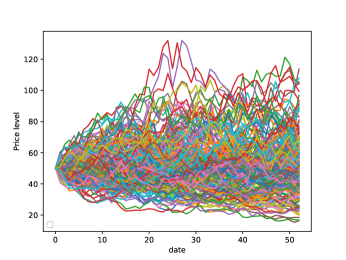
(a) Price

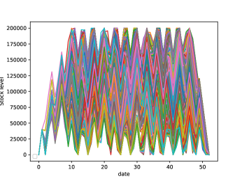
(b) Stock

Figure 2: 200 Spot prices trajectories and stock trajectories associated.

The DCP column permits to show the accuracy of the calculation of the conditional cuts.
Another popular way to value storage consist in using scenario trees. We use a trinomial tree [37] to estimate the solution,with a time step equal to $1/52$. In table 2, we give the result obtained by dynamic programming methods using the bang-bang assumption (DP) and solving a LP problem so using cuts associated with tree to estimate the Bellman value (DPC).

	DP	DPC
Optim Value	1.478	1.478
Simul Value	1.486	1.486

Table 2: Gas storage valuation in millions of numeraire by tree methods

Results obtained by the DP and DPC methods are the same. With the tree method the solution appears to be a little bit higher than with the regression methods. Notice that in the simulation part, uncertainties are sampled on the tree so an error due to the discretization of the tree is present while in the Monte Carlo method with conditional cuts, no discretization error is present. Moreover the approach with a tree is only accurate in very low dimension, as shown in [5].

Next we use the SDDP method with both uncertainties discretized with a trinomial tree and the Monte Carlo method with conditional cuts described in section 3.2. The parameters taken are the following:

• For the SDDP with a tree, the time step is still $1/52$ and we take a number of samples in the forward part equal to $200$ to $4000$.

• For the SDDP with conditional cuts, we take $20000$ trajectories io backward resolution and let the number of mesh vary from $4$ to $6$. The number of samples used in the forward part is taken equal to $28$.

While checking the accuracy of the solution we take $40000$ trajectories in a forward part. For both methods, when a sample gives a new point to explore in the next backward resolution, the cut is only added to the corresponding node in the tree or corresponding cell in the regression method. Moreover no pruning method is used.
Results with the tree method are given on figure 3.

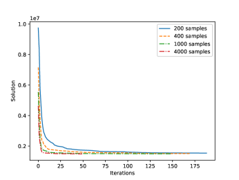
(a) All iterations

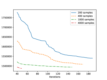
(b) Zoom

Figure 3: Backward value with trees during iterations depending on the number of samples in forward mode.

Using many samples, the backward estimation with trees converges far more quickly. Off course on figure 3, as the number of samples in forward increases we limit the number of iterations as the cost for the resolution explodes. As the number of samples used in forward mode decreases, the convergence rate diminishes dramatically. It is interesting to note that even if the backward resolution is not very accurate, the forward mode gives good results with not too many iterations. For example, using $1000$ samples in the forward mode, we get a forward value of $1.456e06$ at iteration $50$.

Using regressions, we obtain the results illustrated on figure 4.

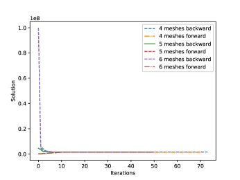
(a) All iterations

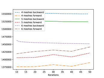
(b) Zoom

Figure 4: Backward value using regressions during iterations depending on the number of meshes.

Using too few meshes, the conditional cuts are not very well estimated : with 4 meshes the interval given by the forward values and the backward value is roughly $[1.36e6,1.54e6]$. Using 5 meshes we get an interval $[1.42e6,1.524e6]$, and using $6$ meshes, we get a tighter estimation $[1.43e6,1.45e6]$.
It is to be noticed that when we use to many meshes for a given number of trajectories used in the backward resolution, the backward value can be below the forward one : in this case either we decrease the number of meshes or increase the number of trajectories used in backward for regressions.
Comparing the cost between an SDDP using trees and an SDDP using regression is not very easy. Tighter bounds between forward and backward values are easier to get with regression when the problem is strongly stochastic. In order to have very good values with trees, we have to use many samples in forward mode to explore rarely reached nodes. This drawback is compensated by the fact that each new node explored only leads to three more LP to solve in backward mode (number of branches of the trinomial tree) at each date.

4.1.2 An artificial test case in higher dimension

In order to test how the method scales as a function of the dimension, we take the same data supposing that we dispose of $n$ similar gas storages that we want to value jointly. Each transition problem is then written as a $n$ dimensional Linear Program solved with COIN CLP. Of course, in this case, the value of $n$ storages is simply $n$ times the value of a single storage.

On figure 5, 6, we plot the convergence of the SDDP scheme for $n=5$ and $n=10$ by giving the value of a single storage estimated as the value of $n$ storages with the SDDP algorithm divided by $n$. A forward estimation of the solution is estimated with $40000$ trajectories every 10 SDDP iterations for the regression method and every 20 SDDP iterations for the tree method. The number of sample used in forward mode is taken equal to $28$ for regressions and $4000$ with trees. As shown in the zoom on the figures, the standard estimation of the solution with Monte Carlo both for tree and regression methods remains rather high with respect to the solution value: oscillations in forward mode are present although the number of trajectories is quite high.

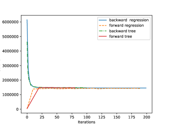
(a) All iterations

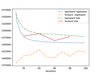
(b) Zoom

Figure 5: Backward and forward values using regressions (6 meshes) and trees during iterations in 5 dimensions.

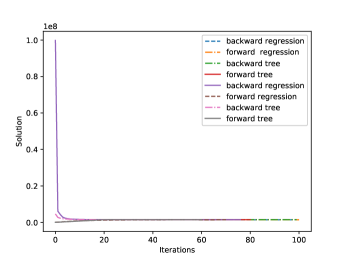
(a) All iterations

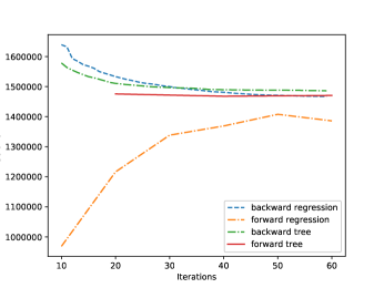
(b) Zoom

Figure 6: Backward and forward values using regressions (6 meshes) and trees during iterations in 10 dimensions.

We note that a direct application of dynamic programming in this situation is simply no longer possible, whereas (our variant of) SDDP scales up very well.
As in the one dimensional case, the value obtained by trees is a little bit higher with the tree method. In dimension 10, the value obtained with regression is slightly below its one dimensional reference ( a value around $1.40e6$ compared to a value of $1.43e6$ obtained in dimension 1).

4.2 A simple storage facility problem facing a consumption constraint

In this section we compare our conditional cut approach with the classical SDDP method (i.e., increasing the state-space) for dealing with uncertainty following an AR(1) model. All experiments are once again achieved with two processors with 14 cores each.

4.2.1 A case in one dimension

In this test case we suppose that the price gas is deterministic so is given by the future price (51). The characteristics of the storage facility are the same as in section 4.1 but we suppose that we have an injection cost per unit of injected gas equal to $0.1$.

The owner of the storage facility is allowed to buy gas on the market and to inject it into the storage (paying the injection cost) but is not allowed to sell it on the market. The gas withdrawn can only be used to satisfy the consumption $D$ following an AR(1) (e.g., [64]) process between two dates $t_{i}=i\frac{T}{N}$ and $t_{i+1}=(i+1)\frac{T}{N}$:

$$D_{i+1}-\tilde{D}_{i+1}=\kappa_{d}(D_{i}-\tilde{D}_{i})+\sigma_{d}\epsilon_{i},$$

where $\epsilon_{i}$ is independent white noise with zero mean and variance 1, $\kappa_{d}$ is set equal to $0.9$, $\sigma_{d}=1000$ and $\tilde{D}$ is an average consumption rate satisfying:

$$\tilde{D}_{i}=22000+7000\sin(4\pi\frac{i}{N}).$$

We denote with $x^{b}_{i}$ the quantity of gas bought at date $t_{i}$, $x^{\tt in}_{i}\in[0,a_{\tt in}]$ the quantity of gas injected and $x^{\tt out}_{i}\in[-a_{\tt out},0]$ the quantity of gas withdrawn. We thus have the following constraint to satisfy at each date $t_{i}$:

$$x^{b}_{i}=D_{i}+x^{in}_{i}+x^{out}_{i}.$$

The following objective function characterizes the cost of a strategy $x^{b}=\left\{x^{b}_{i}\right\}_{i=0,N}$ by the value :

$$J(C_{0},x^{b},D_{0})=\sum_{i=0}^{N}-\phi_{i}(x^{b}_{b}),$$

where $D_{0}$ is the initial consumption value that we suppose to be equal to $\tilde{D}_{0}$ and the optimization problem can be written as

$$J^{*}(C_{0},D_{0})=\inf_{x\in\mathop{U}}J(C_{0},x,D_{0}).$$

Due to the AR(1) structure of the demand, it is possible to add $D_{i}$ to the state vector $x_{i}$ in the algorithm 3.2 as proposed by [51]. We can then test two approaches:

• SDDP with conditional cuts as suggested in section 3.2. Here $x_{i}$ is only the stock level and $\xi_{i}=(D_{i})$ is a dimensional Markov process. All cuts coefficients are one dimensional functions and have to be estimated by one dimensional regressions. In the test case we use $N_{c}^{A}=2000$ trajectories in optimization and conditional cuts coefficients are estimated with an $I_{1}=8$ grid. At each step of the SDDP algorithm we use $8$ forward simulations to discover the new states used in the next backward step.

• SDDP without conditional cuts but with an augmented state vector. Here $x_{i}=(x^{b}_{i},D_{i})$, and at each date $t_{i}$ all cuts coefficients are constant. This method is related to nested Monte Carlo: a set of $N_{i}$ simulations is chosen to simulate $\epsilon_{t}$. So at a given date in the backward pass, we are left with $N_{i}$ LPs to solve for each visited state in the previous forward simulation. It turns out that in order to be able to be able to reach the $0.1\%$ criterium for difference between the forward and the backward iteration, we have to take $N_{i}=2000$. At each step of the SDDP algorithm we use $1$ forward simulation to discover the new states used in the next backward step.

On Figure 7, we give the results obtained by the two approaches until convergence of the backward and forward values to within a given (relative) accuracy of $0.1\%$.

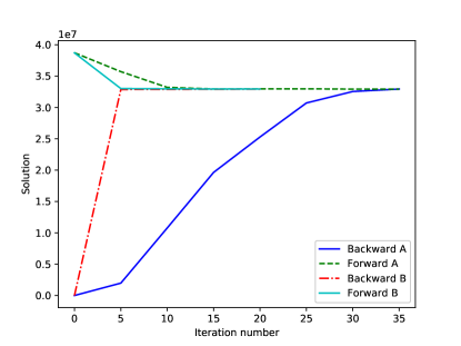
Figure 7: Comparison of optimal values in the backward and forward pass for two variants of SDDP for a load constraint.

Approach A takes 109 seconds to converge while Approach B takes 66 seconds to converge. On this simple case, Approach B is superior to Approach A, especially because of a better convergence rate in the backward step.

4.2.2 Artificial case in dimension 10

In order to test how these methods scale up, we pick the test case of section 4.2.1 but this time with 10 similar storage facilities. We also multiply average load as well as $\sigma_{d}$ by 10. Consequently the expected value of the optimal cost is 10 times the value of the case with one storage facility.

On Figure 8, we give the convergence results obtained by the two approaches.

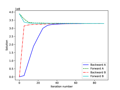
Figure 8: Comparison of optimal values in the backward and forward pass for two variants of SDDP for ten gas storage facilities with a coupling load constraint.

In order to be able to get a relative given accuracy of $0.1\%$ it is necessary to increase $N_{i}$ to $4000$. Both approaches allow us to obtain the same value, showing consistency of the suggested method. Although approach B, obtains a better estimation of the optimal value earlier on in the algorithm, approach A turns out to be faster. Indeed, for reaching a 0.1% asserted gap, Approach A takes $660$ seconds to converge while Approach B takes $775$ (+17%) seconds.

4.3 Valuing a more complex storage facility when facing a consumption constraint

In this section we take the test case 4.2 and allow the prices to vary following the dynamic given in section 4.1. As in the case described in section 4.1, the classical SDDP method cannot deal with this kind of uncertainty. Note that this is so since price uncertainty affects the cost coefficients of the transition problems (e.g., (33)), so that increasing the state space would make these problems bi-linear (i.e., no-longer convex). In the two following subsections we show that our method can deal efficiently with multidimensional uncertainty. All calculation are achieved on a cluster of 8 processors with 14 cores each.

4.3.1 A case in one dimension

Similarly to the sections 4.1 and 4.2 the following objective function characterizes the cost of a strategy $x^{b}=\left\{x^{b}_{i}\right\}_{i=0,N}$:

$$J(C_{0},x^{b},S_{0},D_{0})=\sum_{i=0}^{N}-\phi_{i}(x^{b}_{b}).$$

The optimization problem can be written as

$$J^{*}(C_{0},S_{0},D_{0})=\inf_{x\in\mathop{U}}J(C_{0},x,S_{0},D_{0}).$$

We use the SDDP method with conditional cuts as suggested in section 3.2. Here $x_{i}$ is only the stock level and $\xi_{i}=(S_{i\Delta T},D_{i})$ is a two dimensional Markov process. All cut coefficients are two dimensional functions and have to be estimated by two dimensional regressions. In the test case we use $N_{c}^{A}=32000$ trajectories in optimization and conditional cuts coefficients are estimated with an $(I_{1},I_{2})=(8,4)$ grid (see Figure 1). At each step of the SDDP algorithm we use $32$ forward simulations to discover the new states used in the next backward step.

On Figure 9, we give the results until convergence of the backward and forward values with a given (relative) accuracy of $0.1\%$. The convergence is achieved in 845 seconds.

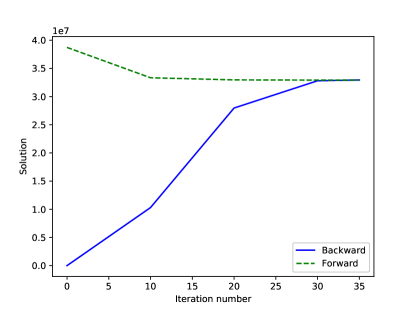
Figure 9: SDDP backward and forward iterations for a gas storage facility with a coupling load constraint.

4.3.2 An artificial test case in dimension 10.

In order to test how the method scales up, we pick the test case of section 4.3.1 but this time with 10 similar storage facilities. We also multiply average load as well as $\sigma_{d}$ by 10. Consequently the expected value of the optimal cost is 10 times the value of the case with one storage facility.

On Figure 10, we give the convergence results obtained by the conditional cuts method.

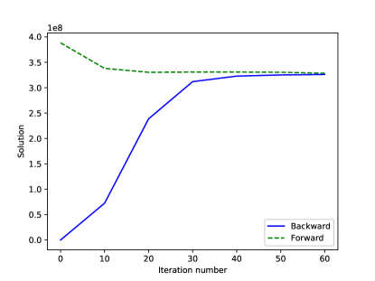
Figure 10: SDDP backward and forward iterations for ten gas storage facilities with a coupling load constraint.

Once again our method converges very efficiently even for a high dimension problem with convergence reached in 2400 seconds.

5 Conclusion

Using conditional cuts we have developed an effective methodology to value easily high dimensional storages problems. Getting rid of building trees for the backward part, the method is easy to use even on a set of initial scenarios, perhaps resulting from historical data, or any other set of scenarios assumed to be Markovian. The method can also be employed whatever the elements of the transition problems impacted by uncertainty. This is not the case for the classic approach, consisting of increasing the state space dimension, the use of which is restricted to right hand side uncertainty.

Moreover, when the dimension of the uncertainties is low and in the special case of auto regressive models, we have shown that the use of conditional cuts is competitive with the classical approach developed in [51] consisting of augmenting the state space to account for past dependency.

At last, because our method is a pure Monte Carlo one, risk optimization such as CVaR or VaR optimization should be much more accurate than classical approaches.

References

- [1] D. Vallad ao, T. Silva, and M. Poggi. Time-consistent risk-constrained dynamic portfolio optimization with transactional costs and time-dependent returns. Annals of Operations Research, 282(1-2):379–405, 2019.
- [2] C. Barrera-Esteve, F. Bergeret, C. Dossal, E. Gobet, A. Meziou, R. Munos, and D. Reboul-Salze. Numerical methods for the pricing of swing options: a stochastic control approach. Methodology and computing in applied probability, 8(4):517–540, 2006.
- [3] J. R. Birge. Decomposition and partitioning methods for multistage stochastic linear programs. Operations Research, 33(5):989–1007, 1985.
- [4] B. Bouchard and N. Touzi. Discrete-time approximation and monte-carlo simulation of backward stochastic differential equations. Stochastic Processes and their applications, 111(2):175–206, 2004.
- [5] B. Bouchard and X. Warin. Monte-Carlo valuation of American options: Facts and new algorithms to improve existing methods. In R. A. Carmona, P. del Moral, P. Hu, and N. Oudjane, editors, Numerical Methods in Finance, volume 12 of Springer Proceedings in Mathematics, pages 215–255. Springer, 2012.
- [6] A. Bruhns, G. Deurveilher, and J.S. Roy. A non-linear regression model for mid-term load forecasting and improvements in seasonality. PSCC 2005 Luik, 2005.
- [7] R. Carmona and M. Ludkovski. Valuation of energy storage: an optimal switching approach. Quantitative Finance, 10(4):359–374, 2010.
- [8] Z. L. Chen and W. B. Powell. Convergent cutting-plane and partial-sampling algorithm for multistage stochastic linear programs with recourse. Journal of Optimization Theory and Applications, 102(3):497–524, 1999.
- [9] V. L. de Matos, D. P. Morton, and E. C. Finardi. Assessing policy quality in a multistage stochastic program for long-term hydrothermal scheduling. Annals of Operations Research, 253(2):713–731, 2017.
- [10] W. de Oliveira, C. Sagastizábal, D. D. Jardim Penna, M. E. P. Maceira, and J. M. Damázio. Optimal scenario tree reduction for stochastic streamflows in power generation planning problems. Optimization Methods and Software, 25(6):917–936, 2010.
- [11] A. R. de Queiroz and D. P. Morton. Sharing cuts under aggregated forecasts when decomposing multi-stage stochastic programs. Operations Research Letters, 41:311–316, 2013.
- [12] C. Donohue and J. R. Birge. The abridged nested decomposition method for multistage stochastic linear programs with relatively complete recourse. Algorithmic Operations Research, 1(1):20–30, 2006.
- [13] J. Dupačová and V. Kozmík. Structure of risk-averse multistage stochastic programs. OR Spectrum, 37(3):559–582, 2015.
- [14] J. Dupačová and J. Polívka. Asset-liability management for czech pension funds using stochastic programming. Annals of Operations Research, 165(1):5–28, 2009.
- [15] J. Dupačová. Portfolio Optimization and Risk Management via Stochastic Programming. Osaka University Press, 2009.
- [16] J. Dupačová, N. Gröwe-Kuska, and W. Römisch. Scenario reduction in stochastic programming : An approach using probability metrics. Mathematical Programming, 95(3):493–511, March 2003.
- [17] A. Eichhorn and W. Römisch. Polyhedral risk measures in stochastic programming. SIAM Journal on Optimization, 16(1):69–95, 2005.
- [18] A. Fahim, N. Touzi, and X. Warin. A probabilistic numerical method for fully nonlinear parabolic pdes. The Annals of Applied Probability, 21(4):1322–1364, 2011.
- [19] B. Fhoula, A. Hajji, and M. Rekik. Stochastic dual dynamic programming for transportation planning under demand uncertainty. In 2013 International Conference on Advanced Logistics and Transport, pages 550–555, May 2013.
- [20] E. Fournié, J-M. Lasry, J. Lebuchoux, and P-L. Lions. Applications of malliavin calculus to monte-carlo methods in finance. ii. Finance and Stochastics, 5(2):201–236, 2001.
- [21] E. Fournié, J-M. Lasry, J. Lebuchoux, P-L. Lions, and N. Touzi. Applications of malliavin calculus to monte carlo methods in finance. Finance and Stochastics, 3(4):391–412, 1999.
- [22] J. Friedman, T. Hastie, and R. Tibshirani. The elements of statistical learning, volume 10 of Springer series in statistics. Springer New York, 2001.
- [23] H. Gevret, J. Lelong, and X. Warin. Stochastic optimization library in c++, 2016.
- [24] P. Girardeau, V. Leclere, and A. B. Philpott. On the Convergence of Decomposition Methods for Multistage Stochastic Convex Programs. Mathematics of Operations Research, 40(1), February 2015.
- [25] E. Gobet, J-P. Lemor, and X. Warin. A regression-based monte carlo method to solve backward stochastic differential equations. The Annals of Applied Probability, 15(3):2172–2202, 2005.
- [26] E. Gobet and P. Turkedjiev. Approximation of backward stochastic differential equations using malliavin weights and least-squares regression. Bernoulli, 22(1):530–562, 2016.
- [27] V. Goel and I. E. Grossmann. A stochastic programming approach to planning of offshore gas field developments under uncertainty in reserves. Computers & Chemical Engineering, 28(8):1409 – 1429, 2004.
- [28] V. Guigues. SDDP for some interstage dependent risk-averse problems and application to hydro-thermal planning. Computational Optimization and Applications, 57(1):167–203, 2014.
- [29] V. Guigues. Convergence analysis of sampling-based decomposition for risk-averse multistage stochastic convex programs. SIAM Journal on Optimization, 26(4):2468–2494, 2016.
- [30] V. Guigues and W. Römisch. Sampling-based decomposition methods for multistage stochastic programs based on extended polyhedral risk measures. SIAM Journal on Optimization, 22(2):286–312, 2012.
- [31] V. Guigues and C. Sagastizábal. The value of rolling horizon policies for risk-averse hydro-thermal planning. European Journal of Operations Research, 217:219–240, 2012.
- [32] H. Heitsch and W. Römisch. Scenario tree generation for multi-stage stochastic programs. In M. Bertocchi, G. Consigli, and M.A.H. Dempster, editors, Stochastic Optimization Methods in Finance and Energy: New Financial Products and Energy Market Strategies, volume 163 of International Series in Operations Research & Management Science, pages 313–341. Springer-Verlag, 2011.
- [33] P. Henaff, I. Laachir, and F. Russo. Gas storage valuation and hedging. a quantification of the model risk. Arxiv, 2013.
- [34] Y. T. Herer, M. Tzur, and E. Yücesan. The multilocation transshipment problem. IIE Transactions, 38(3):185–200, 2006.
- [35] M. Hindsberger and A.B. Philpott. Resa: A method for solving multi-stage stochastic linear programs. In SPIX Stochastic Programming Symposium, Berlin, 2001.
- [36] T. Homem de Mello and B. Pagnoncelli. Risk aversion in multistage stochastic programming: A modeling and algorithmic perspective. European Journal of Operations Research, 249:188–199, 2016.
- [37] J. Hull and A. White. Pricing interest-rate-derivative securities. The review of financiel studies, 3(4):573–592, 1990.
- [38] G. Infanger and D. Morton. Cut sharing for multistage stochastic linear programs with interstage dependency. Mathematical Programming, 75(1):241–256, 1996.
- [39] J. Tsilikis, B. Van Roy. Optimal stopping of Markov processes: Hilbert space theory, approximation algorithms, and application to pricing high dimensional financial derivatives. IEEE Transaction on Automatic Control, 44:1840–1851, 1999.
- [40] J. E. Kelley. The cutting-plane method for solving convex programs. Journal of the Society for Industrial and Applied Mathematics, 8(4):703–712, 1960.
- [41] R. M. Kovacevic and A. Pichler. Tree approximation for discrete time stochastic processes: a process distance approach. Annals of Operations Research, 235(1):395–421, 2015.
- [42] J-P. Lemor, E. Gobet, and X. Warin. Rate of convergence of an empirical regression method for solving generalized backward stochastic differential equations. Bernoulli, 12(5):889–916, 2006.
- [43] K. Linowsky and A.B. Philpott. On the convergence of sampling-based decomposition algorithms for multistage stochastic programs. Journal of Optimization Theory and Applications, 125(2):349–366, 2005.
- [44] F. A. Longstaff and E. S. Schwartz. Valuing american options by simulation: a simple least-squares approach. Review of Financial studies, 14(1):113–147, 2001.
- [45] B. Mo, A. Gjelsvik, and A. Grundt. Integrated risk management of hydro power scheduling and contract management. IEEE Transactions on Power Systems, 16(2):216–221, 2001.
- [46] G. Pagès, H. Pham, and J. Printems. Optimal quantization methods and applications to numerical problems in finance. In Handbook of computational and numerical methods in finance, pages 253–297. Springer, 2004.
- [47] G. Pagès and J. Printems. Optimal quadratic quantization for numerics: the gaussian case. Monte Carlo Methods and Applications, 9(2):135–166, 2003.
- [48] G. Pagès and J. Printems. Functional quantization for numerics with an application to option pricing. Monte Carlo Methods and Applications, 11(4):407–446, 2005.
- [49] G. Pagès and J. Printems. Optimal quantization for finance: from random vectors to stochastic processes. Handbook of Numerical Analysis, 15:595–648, 2008.
- [50] M.V. Pereira, S. Granville, M.H.C. Fampa, R. Dix, and L.A. Barroso. Strategic bidding under uncertainty: A binary expansion approach. IEEE Transactions on Power Systems, 11(1):180–188, February 2005.
- [51] M.V.F. Pereira and L.M.V.G. Pinto. Multi-stage stochastic optimization applied to energy planning. Mathematical Programming, 52(2):359–375, 1991.
- [52] G. Ch. Pflug. Version-independence and nested distributions in multistage stochastic optimization. SIAM Journal on Optimization, 20(3):1406–1420, 2010.
- [53] G. Ch. Pflug and A. Pichler. A distance for multistage stochastic optimization models. SIAM Journal on Optimization, 22(1):1–23, 2012.
- [54] G. Ch. Pflug and W. Römisch. Modeling, Measuring and Managing Risk. World Scientific Publishing Company, 2007.
- [55] A.B. Philpott and V. L. de Matos. Dynamic sampling algorithms for multi-stage stochastic programs with risk aversion. European Journal of Operational Research, 218(2):470 – 483, 2012.
- [56] A.B. Philpott and Z. Guan. On the convergence of stochastic dual dynamic programming and related methods. Operations Research Letters, 36(4):450–455, 2008.
- [57] S. Rebennack. Combining sampling-based and scenario-based nested benders decomposition methods: application to stochastic dual dynamic programming. Mathematical Programming, 156(1):343–389, 2016.
- [58] F. B. Rodríguez, W. de Oliveria, and E. Finardi. Application of scenario tree reduction via quadratic process to medium-term hydrothermal scheduling problem. To appear in IEEE Transactions on Power Systems, 2017.
- [59] A. Ruszczyński and A. Shapiro. Conditional risk mappings. Mathematics of Operations Research, 31(3):544–561, 2006.
- [60] A. Ruszczyński and A. Swietanowski. Accelerating the regularized decomposition method for two stage stochastic linear problems. European Journal of Operational Research, 101(2):328–342, 1997.
- [61] A. Shapiro. Analysis of stochastic dual dynamic programming method. European Journal of Operational Research, 209:63–72, 2011.
- [62] A. Shapiro, D. Dentcheva, and A. Ruszczyński. Lectures on Stochastic Programming. Modeling and Theory, volume 9 of MPS-SIAM series on optimization. SIAM and MPS, Philadelphia, 2009.
- [63] A. Shapiro, W. Tekaya, J. P. da Costa, and M. P. Soares. Risk neutral and risk averse stochastic dual dynamic programming method. European Journal of Operational Research, 224(2):375 – 391, 2013.
- [64] R.H. Shumway and D.S. Stoffer. Time Series Analysis and Its Applications. Springer Texts in Statistics. Springer, 5th edition, 2005.
- [65] Y. Song and J. Luedtke. An adaptive partition-based approach for solving two-stage stochastic programs with fixed recourse. SIAM Journal on Optimization, 25(3):1344–1367, 2015.
- [66] W. van Ackooij, W. de Oliveira, and Y. Song. An adaptive partition-based level decomposition for solving two-stage stochastic programs with fixed recourse. Informs Journal on Computing, 30(1):57–70, 2018.
- [67] W. van Ackooij, W. de Oliveira, and Y. Song. On regularization with normal solutions in decomposition methods for multistage stochastic programs. Computational Optimization and Applications, 74(1):1–42, 2019.
- [68] W. van Ackooij, R. Henrion, A. Möller, and R. Zorgati. Joint chance constrained programming for hydro reservoir management. Optimization and Engineering, 15:509–531, 2014.
- [69] W. van Ackooij and J. Malick. Decomposition algorithm for large-scale two-stage unit-commitment. Annals of Operations Research, 238(1):587–613, 2016.
- [70] X. Warin. Gas storage hedging. In R. A. Carmona, P. del Moral, P. Hu, and N. Oudjane, editors, Numerical Methods in Finance, volume 12 of Springer Proceedings in Mathematics, pages 421–445. Springer, 2012.